Topological Approximate Dynamic Programming under Temporal Logic Constraints

Abstract

In this paper, we develop a model-free approximate dynamic programming method for stochastic systems modeled as Markov decision processes to maximize the probability of satisfying high-level system specifications expressed in a subclass of temporal logic formulas—syntactically co-safe linear temporal logic. Our proposed method includes two steps: First, we decompose the planning problem into a sequence of sub-problems based on the topological property of the task automaton which is translated from a temporal logic formula. Second, we extend a model-free approximate dynamic programming method to solve value functions, one for each state in the task automaton, in an order reverse to the causal dependency. Particularly, we show that the run-time of the proposed algorithm does not grow exponentially with the size of specifications. The correctness and efficiency of the algorithm are demonstrated using a robotic motion planning example.

I INTRODUCTION

Temporal logic is a formal language to describe desired system properties, such as safety, reachability, obligation, stability, and liveness [1]. This paper introduces a model-free Reinforcement Learning (RL) method for stochastic systems modeled as Markov Decision Processes (MDPs), where the planning objective is to maximize the (discounted) probability of satisfying constraints expressed in a subclass of temporal logic— syntactically co-safe LTL (sc-LTL) formulas [2].

Various model checking and probabilistic verification methods for Markov Decision Process (MDP) are model-based [3, 4]. For systems without a model but with a blackbox simulator, RL methods for Linear Temporal Logic (LTL) constraints have been developed with both model-based and model-free methods [5, 6, 7]. A model-based RL learns a model and a near-optimal policy simultaneously. A model-free RL learns only the near-optimal policy from sampled trajectories in the stochastic systems. However, model-free RL methods, such as policy gradient and actor-critic methods [8, 9, 10], face challenges when being used for planning with temporal logic constraints: a LTL formula is translated into a sparse reward signal. The learner receives a reward of $1$ if the constraint is satisfied. This sparse reward provides little gradient information in the policy/value function search. The problem becomes more severe when complex specifications are involved. Consider the following example, a robot needs to visit regions A, B, and C, but if it visits D, then it must visit B before C. If the robot only visits A or B, then it will not receive any reward. When the state space of the MDP is large, a learner not receiving any reward has no way to improve its current policy. To address reward sparsity, reward shaping [11] has been developed. Reward shaping introduces additional reward signals while guaranteeing the policy invariance—the optimal policy remains the same with/without shaping. However, this method has strict requirements for the range of shaping potentials, which is hard to define when LTL constraints are considered.

In this work, we propose a different approach to mitigate the challenges in RL under sparse reward signals in LTL than reward shaping. Our approach is inspired by an idea for efficient value iteration: In an acyclic MDP, there exists an optimal backup order, such that each state in the MDP only needs to perform one-step backup operation in value iteration [12]. In [13], the authors generalize this optimal backup order for acyclic MDPs to general MDPs. They develop a Topological Value Iteration (TVI) method that divides an MDP into Strongly Connected Components (SCCs) and then solves the values of states for each component sequentially in the topological order. Although it seems straightforward to apply TVI to the product MDP, which is obtained by augmenting the original MDP with a finite set of memory states related to the task, the solution suffers from scalability issue. This may be mitigated with the use of Approximate Dynamic Programming (ADP) [14]. The ADP makes the use of value function approximations to approximate the optimal solutions of large-scale problems. Hence, we propose a Topological Approximate Dynamic Programming (TADP) method that includes two stages: Firstly, we translate the task formula into a Deterministic Finite Automaton (DFA) referred as the task DFA, and then exploit the graphical structure in the automaton to determine a topological optimal backup order for a set of value functions—one for each discrete state in the task DFA. Value functions are related by the transitions in the task DFA and jointly determine the optimal policy based on the Bellman equation. Secondly, we introduce function approximations for the set of value functions to reduce the number $N$ of decision variables—the number of states in the product MDP—to a number $M$ of weights in function approximations, where $M\ll N$. Finally, we integrate a model-free ADP with the backup ordering to solve the set of value function approximations, one for each task state, in an optimal order. By doing this, the sparse reward received when the task is completed is propagated back to earlier stages of task completion, which provides meaningful gradient information for the learning algorithm.

Exploiting the structure of task DFAs for planning has been considered in [15] where the authors partition the task DFA into SCCs and then define progress levels towards satisfaction of the specification. In this work, we formally define a topological backup order based on the causal dependency among states in a task DFA. We prove the optimality in this backup order. Further, this backup order can be integrated with the actor-critic method for LTL-constrained planning in [16] or other ADP methods that solve value function approximations to address the sparse reward problem.

The rest of the paper is structured as follows. Section II provides some preliminaries. Section III contains the main results of the paper, including computing the topological order, proof of optimality in this order, and the Topological Approximate Dynamic Programming (TADP) algorithm. The correctness and effectiveness of the proposed method are experimentally validated in the Section IV with a robotic motion planning example. Section V summarizes.

II PRELIMINARIES

Notation: Given a finite set $X$, let $\Delta(X)$ be the set of probability distributions over $X$. The size of the set $X$ is denoted by $\lvert X\rvert$. Let $\Sigma$ be an alphabet (a finite set of symbols). Given $k\in\mathbb{Z}^{+}$, $\Sigma^{k}$ indicates a set of words with length $k$, $\Sigma^{\leq k}$ indicates a set of words with length smaller than or equal to $k$, and $\Sigma^{0}=\lambda$ is the empty word. $\Sigma^{\ast}$ is the set of finite words (also known as Kleene closure of $\Sigma$), and $\Sigma^{\omega}$ is the set of infinite words. $\mathbf{1}_{X}$ is the indicator function with $\mathbf{1}_{X}(x)=1,\text{ if }x\in X$ and $0$ otherwise.

II-A Syntactically co-safe Linear Temporal Logic

Syntactically co-safe LTL formulas [17] are a well-defined subclass of LTL formulas. Given a set of atomic propositions $\mathcal{AP}$, the syntax of sc-LTL formulas is defined as follows:

$$\varphi\coloneqq\mbox{\sf true}\mid p\mid\neg p\mid\varphi_{1}\wedge\varphi_{2}\mid\bigcirc\varphi\mid\varphi_{1}\mbox{$\,{\sf U}\,$}\varphi_{2},$$

where $\varphi,\varphi_{1}$ and $\varphi_{2}$ are sc-LTL formulas, true is the unconditional true, and $p$ is an atomic proposition. Negation ($\neg$), conjunction ($\wedge$), and disconjunction ($\vee$) are standard Boolean operators. A sc-LTL formula can contain temporal operators Next ($\bigcirc$), Until ($\,{\sf U}\,$), and Eventually ($\Diamond$). However, temporal operator Always ($\Box$) is not contained in sc-LTL.

An infinite word with alphabet $2^{\mathcal{AP}}$ satisfying a sc-LTL formula always has a finite-length good prefix [17] . Formally, given a sc-LTL formula $\varphi$ and an infinite word $w=r_{0}r_{1}\cdots$ over alphabet $2^{\mathcal{AP}}$, $w\models\varphi$ if there exists $n\in\mathbb{N}$, $w_{[0:n]}\models\varphi$, where $w_{[0:n]}=r_{0}r_{1}\cdots r_{n}$ is the length $n+1$ prefix of $w$. Thus, an sc-LTL formula $\varphi$ over $2^{\mathcal{AP}}$ can be translated into a DFA $\mathcal{A}_{\varphi}=\langle Q,\Sigma,\delta,q_{0},F\rangle$, where $Q$ is a finite set of states, $\Sigma=2^{\mathcal{AP}}$ is a finite set of symbols called the alphabet, $\delta:Q\times\Sigma\rightarrow Q$ is a transition function, $q_{0}\in Q$ is an initial state, and $F\subseteq Q$ is a set of accepting states. A transition function is recursively extended in the general way: $\delta(q,aw)=\delta(\delta(q,a),w)$ for given $a\in\Sigma$ and $w\in\Sigma^{\ast}$. A word $w=uv$ is accepting if and only if $\delta(q,u)\in F$. DFA $\mathcal{A}_{\varphi}$ accepts the set of words satisfying $\varphi$.

We consider stochastic systems modeled as MDPs. We introduce a labeling function to relate paths in an MDP $M$ to a given specification described by an sc-LTL formula.

Definition II.1 (Labeled MDP).

A labeled MDP is a tuple $M=\langle S,A,s_{0},P,\mathcal{AP},L\rangle$, where $S$ and $A$ are finite state and action sets, $s_{0}$ is the initial state, the transition probability function $P(\cdot\mid s,a)\in\Delta(S)$ is defined as a probability distribution over the next state given action is taken at the current state, $\mathcal{AP}$ denotes a finite set of atomic propositions, and $L:S\rightarrow 2^{\mathcal{AP}}$ is a labeling function mapping each state to the set of atomic propositions true in that state.

A finite-memory stochastic policy in the MDP is a function $\pi:S^{\ast}\rightarrow\Delta(A)$ that maps a history of state sequence into a distribution over actions. A Markovian stochastic policy in the MDP is a function $\pi:S\rightarrow\Delta(A)$ that maps the current state into a distribution over actions. Given an MDP $M$ and a policy $\pi$, the policy induces a Markov chain $M^{\pi}=\{s_{t}\mid t=0,\dots,\infty\}$ where $s_{i}$ is the random variable for the $i$-th state in the Markov chain $M^{\pi}$, and it holds that $s_{i+1}\sim P(\cdot\mid s_{i},a_{i})$ and $a_{i}\sim\pi(\cdot\mid s_{0}s_{1}\ldots s_{i})$.

Given a finite (resp. infinite) path $\rho=s_{0}s_{1}\ldots s_{N}\in S^{\ast}$ (resp. $\rho\in S^{\omega}$), we obtain a sequence of labels $L(\rho)=L(s_{0})L(s_{1})\ldots L(s_{N})\in\Sigma^{\ast}$ (resp. $L(\rho)\in\Sigma^{\omega}$). A path $\rho$ satisfies the formula $\varphi$, denoted by $\rho\models\varphi$, if and only if $L(\rho)$ is accepted by $\mathcal{A}_{\varphi}$. Given a Markov chain induced by policy $\pi$, the probability of satisfying the specification, denoted by $P(M^{\pi}\models\varphi)$, is the expected sum of the probabilities of paths satisfying the specification.

$$P(M^{\pi}\models\varphi)\coloneqq\mathop{\bf E{}}\left[\sum_{t=0}^{\infty}\mathbf{1}(\rho_{t}\models\varphi)\right],$$

where ${\rho}_{t}=s_{0}s_{1}\ldots s_{t}$ is a path of length $t+1$ in $M^{\pi}$.

Problem 1.

Given a labeled MDP $M$ and an sc-LTL formula $\varphi$, we can have a product MDP $\mathcal{M}$. The MaxProb problem is to synthesize a policy $\pi$ that maximizes the probability of satisfying $\varphi$. Formally,

$$\pi^{\ast}=\arg\max_{\pi}P(M^{\pi}\models\varphi).$$

Definition II.2 (Product MDP).

Given a labeled MDP $M=\langle S,A,s_{0},P,\mathcal{AP},L\rangle$, an sc-LTL formula $\varphi$ with the corresponding DFA $\mathcal{A}_{\varphi}=\langle Q,\Sigma,\delta,q_{0},F\rangle$, the product of $M$ and $\mathcal{A}_{\varphi}$ is denoted by $M\otimes\mathcal{A}_{\varphi}=\langle S\times Q,(s_{0},\delta(q_{0},L(s_{0})),S\times F,A,\delta,R\rangle$ with (1) a set of states, $S\times Q$, (2) an initial state, $(s_{0},\delta(q_{0},L(s_{0}))$, (3) the set of accepting states, $S\times F$, (4) the transition function defined by $P(((s^{\prime},q^{\prime}),a^{\prime})\mid(s,q),a)=P(s^{\prime}\mid s,a)\mathbf{1}_{\{q^{\prime}\}}(\delta(q,L(s)))$, (5) the reward function $R:S\times Q\times A\rightarrow[0,1]$. Formally,

$$R((s,q),a)=\sum_{(s^{\prime},q^{\prime})} P((s^{\prime},q^{\prime})\mid(s,q),a)\cdot\mathbf{1}_{F}(q^{\prime}).$$ (1)

We let all states in $S\times F$ sink/absorbing states, i.e., for any $(s,q)\in S\times F$, for any $a\in A$, $P((s,q)|(s,q),a)=1$ and $R((s,q),a)=0$. For clarity, we denote this product MDP by $\mathcal{M}_{\varphi}$, i.e., $\mathcal{M}_{\varphi}=M\otimes\mathcal{A}_{\varphi}$. When the specification $\varphi$ is clear from the context, we denote the product MDP by $\mathcal{M}$.

By definition, the path will receive a reward of $1$ if it ends in the set of accepting states $S\times F$. The total expected reward given a policy $\pi$ is the probability of satisfying the formula $\varphi$. By maximizing the total reward we find an optimal policy for the MaxProb problem. In practice, we are often interested in maximizing a discounted total reward, which is the discounted probability of satisfying $\varphi$.

The planning problem is to solve the optimal value function and policy function satisfying

$$\begin{split}&V((s,q))=\tau\log\sum_{a}\exp(R((s,q),a)\\ &\qquad+\gamma\sum_{s^{\prime},q^{\prime}}P((s^{\prime},q^{\prime})\mid(s,q),a)V((s^{\prime},q^{\prime})))/\tau),\\ &Q((s,q),a)=R((s,q),a)+\gamma\mathop{\bf E{}}_{(s^{\prime},q^{\prime})}V((s^{\prime},q^{\prime})),\\ &\pi(a\mid(s,q))=\exp((Q((s,q),a)-V((s,q)))/\tau),\end{split}$$ (2)

where $\tau$ is an user-specified temperature parameter and $\gamma$ is a discounting factor. We use the softmax Bellman operator [18] instead of the hardmax Bellman operator [19]. Value Iteration (VI) can solve the optimal value function in the product MDP and converges in the polynomial time of the size of the state space, i.e., $\lvert S\times Q\rvert$. However, VI is model-based and difficult to scale to large planning problems with complex specifications.

III MAIN RESULT

We are interested in developing model-free RL algorithms for solving the MaxProb problem. However, if we directly solve for approximately optimal policies in the product MDP using the method in Section III-B, as the reward is sparse, it becomes a rare event to sample a path satisfying the specification. As a consequence, the estimate of the gradient in [14] has a high variance with finite samples. To address this problem, we develop Topological Approximate Dynamic Programming (TADP) that leverages the structure property in the task automaton to improve the convergence due to sparse and temporally extended rewards with LTL specifications.

III-A Hierarchical decomposition and causal dependency

First, it is observed that given temporally extended goals, we can partition the product state space based on the discrete automaton states referred as discrete modes. The following definitions are generalized from almost-sure invariant set [20] in Markov chains to that in MDPs.

Definition III.1 (Invariant set and guard set).

Given a DFA mode $q\in Q$ and an MDP $M$, the invariant set of $q$ with respect to $M$, denoted by $\mathsf{\bf Inv}(q,M)$, is a set of MDP states such that no matter which action is selected, the system has probability one to stay within the mode $q$. Formally,

$$\mathsf{\bf Inv}(q,M)= \{s\in S\mid\forall a\in A,\forall s^{\prime}\in S,P(s^{\prime}\mid s,a)>0$$

$$\implies\delta(q,L(s^{\prime}))=q\},$$ (3)

where $\implies$ means implication.

Given a pair $(q,q^{\prime})$ of DFA states, where $q\neq q^{\prime}$, the set of guard states of the transition from $q$ to $q^{\prime}$, denoted by $\mathsf{\bf Guard}(q,q^{\prime},M)$, is a subset of $S$ in which a transition from $q$ to $q^{\prime}$ may occur. Formally,

$$\mathsf{\bf Guard}(q,q^{\prime},M)=\{s\in S\mid\exists a\in A,\exists s^{\prime}\in S,$$

$$P(s^{\prime}\mid s,a)>0\land\delta(q,L(s^{\prime}))=q^{\prime}\}.$$ (4)

When the MDP $M$ is clear from the context, we refer $\mathsf{\bf Inv}(q,M)$ to $\mathsf{\bf Inv}(q)$ and $\mathsf{\bf Guard}(q,q^{\prime},M)$ to $\mathsf{\bf Guard}(q,q^{\prime})$.

Next, we define causal dependency between modes: In the product MDP $\mathcal{M}$, a state $(s_{1},q_{1})$ is causally dependent on state $(s_{2},q_{2})$, denoted by $(s_{1},q_{1})\rightarrow(s_{2},q_{2})$, if there exists an action $a\in A$ such that $P((s_{2},q_{2})\mid(s_{1},q_{1}),a)>0$. This causal dependency is initially introduced in [13] and generalized to the state space of the product MDP.

According to Bellman equation (5), if there exists a probabilistic transition from $(s_{1},q_{1})$ to $(s_{2},q_{2})$ in the product MDP, then the value $V(s_{1},q_{1})$ depends on the value $V(s_{2},q_{2})$.

Two states can be causally dependent on each other. In that case, we say that these two states are mutually causally dependent. Next, we lift the causal dependency from product MDP to the task DFA, by introducing casually dependent modes.

Definition III.2 (Causally dependent modes).

A mode $q_{1}$ is causally dependent on mode $q_{2}$ if and only if $\mathsf{\bf Guard}(q_{1},q_{2})\neq\emptyset$, that is, there exists a transition in the product MDP from a state in mode $q_{1}$ to a state in mode $q_{2}$. A pair of modes $(q_{1},q_{2})$ is mutually causally dependent if and only if $q_{1}$ is causally dependent on $q_{2}$ and $q_{2}$ is causally dependent on $q_{1}$.

Definition III.3 (Meta-mode).

A meta mode $X\subseteq Q$ is a subset of modes that are mutually causally dependent on each other. If a mode $q$ is not mutually causally dependent on any other modes, then the set $\{q\}$ itself is a meta mode. A meta mode $X$ is maximal if there is no other mode in $Q\setminus X$ that is mutually causally dependent on a mode in $X$.

Definition III.4 (The maximal set of Meta-modes).

$\cal X$ is said to be the set of maximal meta modes in the product MDP if and only if it satisfies: i) any set $X\in\cal X$ is a maximal meta mode, ii) the union of sets in $\cal X$ yields the set $Q$, i.e., $\cup_{X\in\mathcal{X}}X=Q$.

Lemma III.1.

The maximal set $\cal X$ of meta modes is a partition of $Q$.

Proof.

By the way of contradiction, suppose $\cal X$ is not a partition of $Q$, then there exists a mode $q\in X\cap X^{\prime}$. Because $q$ is mutually causally dependent on all modes in $X$ as well as $X^{\prime}$, then any pair $(q_{1},q_{2})\in X\times X^{\prime}$ will be mutually causally dependent—a contradiction to the definition of $\cal X$. ∎

We denote $X\rightarrow X^{\prime}$ if a mode $q\in X$ is causally dependent on mode $q^{\prime}\in X^{\prime}$. By the transitivity property, if $X_{1}\rightarrow X_{2}$ and $X_{2}\rightarrow X_{3}$, then we denote the causal dependency of $X_{1}$ on $X_{3}$ by $X_{1}\rightarrow^{+}X_{3}$. The following lemma states that two states in the product MDP are causally dependent if their discrete modes are causally dependent.

Lemma III.2.

Given two meta-modes $X,X^{\prime}\in\mathcal{X}$, if $X\rightarrow^{+}X^{\prime}$ but not $X^{\prime}\rightarrow^{+}X$, then for any state $(s,q)\in S\times X$ and $(s^{\prime},q^{\prime})\in S\times X^{\prime}$, it is the case that either $(s,q)\rightarrow^{+}(s^{\prime},q^{\prime})$ or these two states are causally independent.

Proof.

By the way of contradiction, if $(s,q)$ and $(s^{\prime},q^{\prime})$ are causally dependent and $(s^{\prime},q^{\prime})\rightarrow^{+}(s,q)$, then there must exist a state $(s^{\prime\prime},q^{\prime\prime})$ such that $(s^{\prime},q^{\prime})\rightarrow^{+}(s^{\prime\prime},q^{\prime\prime})$ and $(s^{\prime\prime},q^{\prime\prime})\rightarrow(s,q)$. Relating the causal dependency of states in the product MDP and the definition of guard set, we have $s^{\prime\prime}\in\mathsf{\bf Guard}(q^{\prime\prime},q)$ and $q^{\prime\prime}\rightarrow q$. Further $q^{\prime}\rightarrow^{+}q^{\prime\prime}\rightarrow q$, thus $X^{\prime}\rightarrow^{+}X$, which is a contradiction as $X^{\prime}\not\rightarrow^{+}X$. ∎

Lemma III.2 provides structural information about topological value iteration (TVI). If $X\rightarrow^{+}X^{\prime}$ and $X^{\prime}\not\rightarrow^{+}X$, then based on TVI, we shall update the values for states in the set $\{(s,q)\mid q\in X^{\prime}\}$ before updating the values for states in the set $\{(s,q)\mid q\in X\}$.

However, the causal dependency in meta-modes does not provide us with a total order over the set of maximally meta modes because two meta modes can be causally independent. A total order is needed for deciding the order in which the optimal value functions for modes are updated.

To obtain a total order, we construct a total ordered sequence of sets of maximal meta modes. Given the set of maximal meta-modes $\cal X$,

1. Let $\mathcal{L}_{0}=\{X\in{\cal X}\mid X\cap F\neq\emptyset\}$ and $i=1$.

2. Let $\mathcal{L}_{i}=\{X\in{\cal X}\setminus\cup_{k=0}^{i-1}\mathcal{L}_{k}\mid\exists X^{\prime}\in\mathcal{L}_{i-1}\text{ such that }X\rightarrow X^{\prime}\}$, and increase $i$ by 1

3. Repeat until $i=n$ and $\mathcal{L}_{n+1}=\emptyset$.

We refer $\{\mathcal{L}_{i}\mid i=0,\ldots,n\}$ as level sets over meta modes. Based on the definition of set $\{\mathcal{L}_{i}\mid i=0,\ldots,n\}$, we let $\rightsquigarrow$ define an ordering on level sets as follows: $\mathcal{L}_{i}\rightsquigarrow\mathcal{L}_{i-1}\mid i=1,\ldots,n$. We give the following two statements.

Lemma III.3.

If there exists $X\in\mathcal{X}$ such that $X\not\in\mathcal{L}_{i}$ for any $i=0,\ldots,n$, then the set of states in $X$ is not coaccessible from the final set $F$ of states in DFA $\mathcal{A}_{\varphi}$.

Proof.

By construction, this meta mode $X$ is not causally dependent on any meta mode that contains $F$. Thus, it is not coaccessible in the task DFA $\mathcal{A}_{\varphi}$, i.e., there does not exist a word $w$ such that $\delta(q,w)\in F$ for some $q\in X$. ∎

If a DFA is coaccessible, then we have $\cup_{i=0}^{n}\mathcal{L}_{i}=\mathcal{X}$. A state $q$ that is not coaccessiable from the final set $F$ should be trimmed before planning because the value $V(s,q)$ for any $s\in S$ will not be used for optimal planning in the product MDP to reach $F$.

Proposition III.1.

The ordering $\rightsquigarrow$ is a total order:

$$\mathcal{L}_{n}\rightsquigarrow\mathcal{L}_{n-1}\ldots\rightsquigarrow\mathcal{L}_{0}.$$

Theorem III.4 (Optimal Backup Order [12]).

If an MDP is acyclic, then there exists an optimal backup order. By applying the optimal order, the optimal value function can be found with each state needing only one backup.

We generalize the Optimal Backup Order on an acyclic MDP to the product MDP as the following:

Theorem III.5 (Generalized optimal backup order for hierarchical planning).

Given the optimal planning problem in the product MDP and the causal ordering of meta modes, by updating the value functions of all meta-modes in the same level set, in a sequence reverse to the ordering $\rightsquigarrow$, the optimal value function for each meta mode can be found with only one backup, i.e., solving the value function of that meta mode using value iteration or an ADP method that solves the value function approximation.

Proof.

We show this by induction. Suppose there exists only one level set, the problem is reduced to optimal planning in a product MDP with only one update for value functions of meta-modes in this level set. When there are multiple level sets, each time the optimal planning performs value function update for one level set. The value $V(s,q)$ for $q\in X$ only depends on the values of its descent states, that is, $\{V(s^{\prime},q^{\prime})\mid(s,q)\rightarrow(s^{\prime},q^{\prime})\}$. It is noted that the mode $q^{\prime}$ of any descendant $(s,q)$ must belong to either meta-modes $X$, or some $X^{\prime}\in\mathcal{X}$ such that $X\rightarrow^{+}X^{\prime}$. By definition of level sets, if $X\in\mathcal{L}_{i}$, then $X^{\prime}\in\mathcal{L}_{k}$ for some $k\leq i$. It means the value $V(s^{\prime},q^{\prime})$ for any descendant $(s,q)$ is either updated in level $\mathcal{L}_{k}$, $k<i$, or along with the value $V(s,q)$, when $k=i$. As a result, after the value functions $\{V(\cdot,q)\mid q\in X,X\in\mathcal{L}_{i}\}$ converge, the Bellman residuals of states in $\{(s,q)\mid q\in X,X\in\mathcal{L}_{k},k\leq i\}$ remain unchanged, while the value functions of meta-modes in other level sets with higher levels are updated. Thus, each mode only needs to be updated once. ∎

Example III.1.

We use a simple example to illustrate. Given a system-level specification: $\Diamond(b\land\bigcirc\Diamond c)\land\Diamond(a\land\bigcirc\Diamond d)$, the corresponding DFA is shown in Fig. 1. In this DFA, each state is its own meta mode $X_{i}=\{q_{i+1}\},i=0,\ldots 8$. Different level sets $\mathcal{L}_{i},i=0,\ldots,4$, are contained in different styled ellipses.

Figure 1: DFA with respect to $\Diamond(b\land\bigcirc\Diamond c)\land\Diamond(a\land\bigcirc\Diamond d)$.

III-B Model-free ADP for planning with temporal logic constraints

ADP makes use of value function approximations to solve for Problem 1. First, let’s define the softmax Bellman operator by

$$\mathcal{B}V(s,q)=\tau\log\sum_{a}\exp((R((s,q),a)\\ +\gamma\sum_{(s^{\prime},q^{\prime})}P((s^{\prime},q^{\prime})\mid(s,q),a)V(s^{\prime},q^{\prime}))/\tau),$$ (5)

where $\tau>0$ is an user-specified temperature parameter.

We introduce a mode-dependent value function approximation as follows: For each $q\in Q$, the value function is approximated by $V(\cdot;\theta_{q}):S\rightarrow\mathbb{R}$ where $\theta_{q}\in\mathbb{R}^{\ell_{q}}$ is a parameter vector of length $\ell_{q}$. We use a linear function approximation of $V(\cdot;\theta_{q})=\sum_{k=1}^{\ell_{q}}\phi_{k,q}(\cdot)\theta_{q}[k]=\Phi_{q}\theta_{q}$, where $\phi_{k,q}:S\rightarrow\mathbb{R},k=1,\dots,\ell_{q}$ are pre-selected basis functions. We first define two sets: For meta-modes $X,X^{\prime}\in\mathcal{X}$, let

$$\mathsf{\bf Inv}(X)=\bigcup_{q\in X}\mathsf{\bf Inv}(q),\quad\text{ and}$$

$$\mathsf{\bf Guard}(X,X^{\prime})=\bigcup_{q\in X,q^{\prime}\in X^{\prime}}\mathsf{\bf Guard}(q,q^{\prime}).$$

Given the level sets $\{\mathcal{L}_{i}\mid i=0,\ldots,n\}$, the computation of value function approximation for each DFA mode is carried out in the order of level sets.

1. Starting with level $0$, let $i=0$ and $V((s,q);\theta_{q})=1$ (see Remark 2) for all $s\in S$ and $q\in F$. For each $X\in\mathcal{L}_{0}$, we solve an ADP problem:

   $$\min_{\{\theta_{q}\mid q\in X\setminus F\}} \sum_{(s,q)\in S\times X}c(s,q)V((s,q);\theta_{q}),$$ (6)

   subject to: $$\mathcal{B}V((s,q);\theta_{q})-V((s,q);\theta_{q})\leq 0,$$

   $$\forall s\in\mathsf{\bf Inv}(X)\bigcup\left(\cup_{X^{\prime}\in\mathcal{X}}\mathsf{\bf Guard}(X,X^{\prime})\right),$$

   where parameters $c(s,q)$ are state relevant weights. All states $\{(s,q)\mid q\in F\}$ are absorbing with values of $1$. The reward function $R((s,q),a)=0$ for all $s\in S$, $q\in X$, and $a\in A$. After solving the set of value functions $\{V(s,q;\theta_{q})\mid q\in X,X\in\mathcal{L}_{0}\}$. The solution of this ADP is proven to be a tight upper bound of the optimal value function [14]. See Appendix for more information about this ADP method.

2. Let $i\leftarrow i+1$.

3. At the $i$-th step, given the value $\{V(s,q;\theta_{q})\mid q\in X\land X\in\mathcal{L}_{k},k<i\}$, we solve, for each $X\in\mathcal{L}_{i}$, an ADP problem stated as follows:

   $$\min_{\{\theta_{q}\mid q\in X\}} \sum_{(s,q)\in S\times X}c(s,q)V((s,q);\theta_{q}),$$ (7)

   subject to: $$\mathcal{B}V((s,q);\theta_{q})-V((s,q);\theta_{q})\leq 0,$$

   $$\forall s\in\mathsf{\bf Inv}(X)\bigcup\left(\cup_{X^{\prime}\in\mathcal{X}}\mathsf{\bf Guard}(X,X^{\prime})\right),$$

   where $V((s^{\prime},q^{\prime});\theta_{q^{\prime}})$ to be solved either has $q^{\prime}\in X$ or $q^{\prime}\in X^{\prime}$ for some $X^{\prime}\in\mathcal{L}_{k}$, $k<i$. Note that by Theorem III.5, the meta-mode $X^{\prime}$, for which $\mathsf{\bf Guard}(X,X^{\prime})$ is nonempty, cannot be in a level set higher than $i$. When $q^{\prime}\in X^{\prime}$ and $X^{\prime}\in\mathcal{L}_{i}$, then $\theta_{q^{\prime}}$ is a decision variable for this ADP. When $q^{\prime}\in X^{\prime}$ and $X^{\prime}\in\mathcal{L}_{k}$ for some $k<i$, then the value $V((s^{\prime},q^{\prime});\theta_{q^{\prime}})$ is computed in previous iterations and substituted. A state $(s^{\prime},q^{\prime})$ whose value is determined in previous iterations is made absorbing in this iteration. The reward function $R((s,q),a)=0$ for all $s\in S$, $q\in X$, and $a\in A$.

4. Repeat step $2,3$ until $i=n$. Return the set $\{V(s,q;\theta_{q})\mid q\in Q\}$. The policy is computed using the softmax Bellman operator, defined in (2) by substituting the value function $V(s,q)$ with its approximation $V((s,q);\theta_{q})$.

Remark 1.

The problem solved by ADP is essentially a stochastic shortest path problem [21]. For such a problem, two approaches can be used: One is to fix the values of states to be reached and assign the reward to be zero. During value iteration, the value of the states to be reached will be propagated back to the values of other states. The aforementioned reward design and ADP formulation use the first approach. Another way to introduce a reward function defined by $R((s,q),a)=\sum_{s^{\prime},q^{\prime}}P((s^{\prime},q^{\prime})\mid(s,q),a)R((s^{\prime},q^{\prime}))$, where $R(s^{\prime},q^{\prime})=V((s^{\prime},q^{\prime});\theta_{q^{\prime}})$ if $q\in X$, $q^{\prime}\in X^{\prime}$, $X\rightarrow X^{\prime}$ , and $R(s^{\prime},q^{\prime})=0$ otherwise.

Remark 2.

A value iteration using the softmax Bellman operator finds a policy that maximizes a weighted sum of total rewards and the entropy of policy (see [18] for more details). When the value/reward is small, the total entropy of policies accumulated with the softmax Bellman operator overshadows the value given by the reward function. This is called the value diminishing problem. Thus, for both cases, when the value $V((s^{\prime},q^{\prime});\theta_{q^{\prime}})$ of the state to be reached is small, we scale this value by a constant $\alpha$ to avoid the value diminishing problem. Given the nature of the MaxProb problem, with a reward of 1 being assigned when the LTL constraint is satisfied, we almost always need to amplify the reward to avoid the value diminishing problem.

IV CASE STUDY

We validate the algorithm in a motion planing problem under a sc-LTL specification in a grid world. In this example, we consider the following specification: $\Diamond(((A\land(\neg B\mbox{$\,{\sf U}\,$}C))\lor(B\land(\neg A\mbox{$\,{\sf U}\,$}D)))\land\Diamond\mathsf{goal}\land\Box\neg O)$, and the corresponding DFA is plotted in Fig. 3. This specification describes that the system visits A, C, and goal sequentially, or the system visits B, D, and goal sequentially, while avoiding obstacles. Regions $A,B,C,D$, obstacles $O$, and goal are shown in Fig. 2. The partitions of meta modes are shown in Fig. 3 with different meta modes being boxed in different styled rectangles. The task automaton is partitioned into four meta modes $X_{i},i=0,\ldots,3$, and each level set $\mathcal{L}_{i},i=0,\ldots,3$, contains one meta mode with the same index. The reward is defined as the following: the robot receives a reward of $60$ (an amplified reward to avoid value diminishing) if the trajectory satisfies the specification. In each state $s\in S$ and for robot’s different actions (heading up (’U’), down (’D’), left(’L’), right(’R’)), the probability of arriving at the correct cell is $1-0.03\times\lvert N\rvert$, and the probability of arriving a wrong cell is $0.03$, where $0.03$ is the randomness in the system and $\lvert N\rvert$ is the number of possible succeeding states. We surround the gird world with walls. If the system hits the wall, it will be bounced back and stay at its original cell. All the obstacles are sink states, i.e., when a robot goes to an obstacle—it stays there forever.

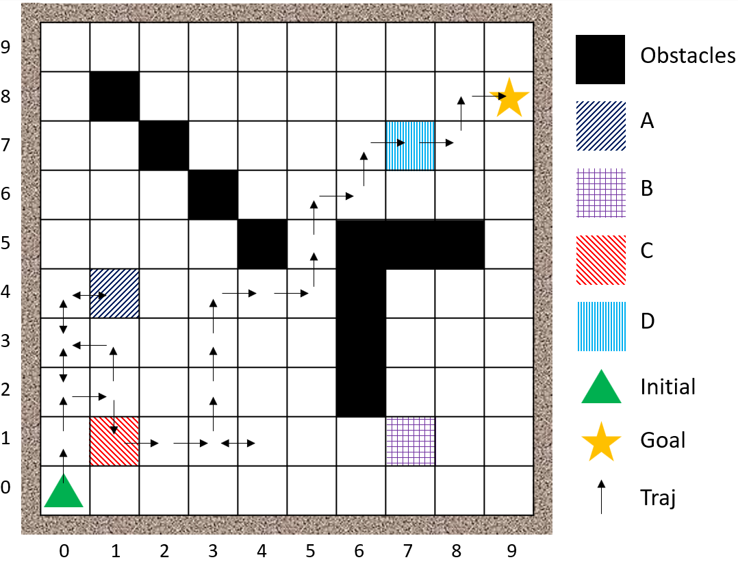
Figure 2: One simulation on the grid world.

Figure 3: Automaton $\Diamond(((A\land(\neg B\mbox{$\,{\sf U}\,$}C))\lor(B\land(\neg A\mbox{$\,{\sf U}\,$}D)))\land\Diamond\mathsf{goal}\land\Box\neg O)$. Meta modes and the level sets are marked.

The planning objective is to find an approximately optimal policy for satisfying the specification with a maximal probability. We compare the TADP with VI and TVI to show the correctness and efficiency.

Parameters

We use the following parameters: the user-specified temperature is $\tau=2$, discounting factor is $\gamma=0.9$, and error tolerance is $\epsilon=10^{-3}$. The tolerance is shared by TVI, VI, and TADP, where the stopping criterion is $\|\max(V^{j}(s)-V^{j-1}(s))\|\leq\epsilon$ for $j$-th iteration of in TVI and VI and for each inner $j$-th iteration of TADP, respectively.

We adopt the following initial parameters in the TADP algorithm for the $k$-th problem (see appendix for the meanings of parameters): the coefficient of the penalty is $b=1.5$, the learning rate is $\eta=0.1$, the penalty parameter is $\nu=2.0$, and the Lagrangian multipliers is $\lambda=0$. During each inner iteration, we sample $30$ trajectories of length $\leq 3$. The value function $V(\cdot;\theta_{q})$ is approximated by a weighted sum of Gaussian Kernels: $V(\cdot;\theta_{q})=\Phi_{q}\theta_{q}$, where basis functions $\Phi_{q}=[\phi_{1},\phi_{2},\ldots,\phi_{\ell_{q}}]^{\intercal}$ are defined as the following: $\Phi_{j}(s)=K(s,c^{(j)})$ and $K(s,s^{\prime})=\exp(-\frac{SP(s,s^{\prime})^{2}}{2\sigma^{2}}),$ where $\{c^{(j)},j=1,\ldots,\ell_{q}\}$ is a set of pre-selected centers and $\sigma=1$. In this example, we select the centers to be uniformly selected points with interval $1$ within the grid world.

After the TADP converges, we obtain the policy from the converged value functions computed by TADP and simulate the system. We plot one simulation of the system in Fig. 2. The system starts at the initial state $s_{init}$, then it visits region $A$ then region $C$, eventually it visits the goal state $s_{goal}$.

Value Comparison

In Fig. 4, we plot the heatmaps and values for different states at $q_{3}$ obtained by VI, TVI, and TADP. In heatmaps, the brighter the area is, the higher value of that area is. The results from Fig. 4(a) and  4(b) shows that VI and TVI both show the most bright area is at $(7,7)$. In Fig. 4(c), the area around $(7,7)$ obtained has relatively bright color. The heatmap of TADP is not exactly the same as the other two. This is due to the approximation error. Comparing three value surfs in Fig. 4(d),  4(e), and  4(f), we are able to see the similarity between these three value surfs.

(a)

(b)

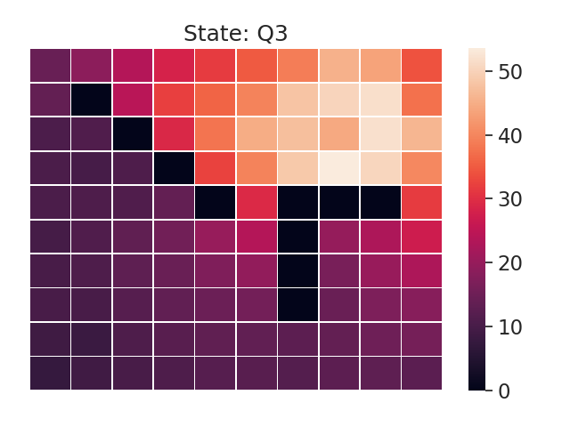
(c)

(d)

(e)

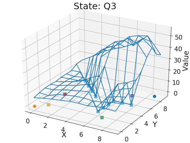
(f)

Figure 4: Comparison between VI, TVI, TADP for different states at $q_{3}$: (a) (b) (c) are the heatmaps of $V(\cdot,q_{3})$ obtained by VI, TVI, and TADP, respectively. (d) (e) (f) are the corresponding value surfs of $V(\cdot,q_{3})$ obtained by VI, TVI, and TADP, respectively.

Run-time

We conduct two experiments for different sizes of grid worlds, i.e., $10\times 10$ and $20\times 20$. We show the results in Table I. In different sizes of gird worlds, comparing VI and TVI run-times are reduced by $38.45\%$ and $53.62\%$ by exploiting the topological structure, and the total numbers of Bellman Backup Operations are reduced by $7.71\%$ and $7.76\%$. In terms of simple specifications, the decomposition occupies major CPU time, but exploiting the topological structure will be leveraged if more complex specifications are associated. The TADP converges after $135.96$ seconds and $1117.91$ seconds, respectively for different sizes of grid worlds. The run-times of the TVI and VI in a $20\times 20$ grid world are $14$-$20$ times their run-times in the $10\times 10$ grid world. However, the run-time of TADP in a $20\times 20$ grid world is only $8$ times the run-time of TADP in the $10\times 10$ grid world. TADP is more beneficial in large MDP problems or with more complex specifications. It is noted that though TADP takes in general longer time to converge, but it is model-free. TVI and VI are model-based.

Algorithms		VI	TVI	TADP
$10\times 10$	Bellman Backup Operations (times)	64620	59636	N/A
	Run-time (Seconds)	11.52	7.09	135.96
$20\times 20$	Bellman Backup Operations (times)	280620	258836	N/A
	Run-time (Seconds)	222.56	103.21	1117.59

TABLE I: Bellman Backup Operations and Run-times between VI, TVI, and TADP. Note that TVI has a significantly shorter run-time.

Convergence

In Fig. 5, we plot the convergence of values for different states in the $10\times 10$ grid and modes in automaton against epochs, which is the number of inner iterations in TADP. It indicates that the values initially oscillate, but all values converge after $250$ iterations.

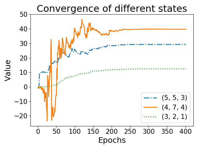
Figure 5: The convergence of values in TADP in the $10\times 10$ stochastic grid world for different states in the product MDP. A product state $(5,5,3)$ means the grid cell $(5,5)$ and the DFA state $q_{3}$.

Statistical Results

We want to quantify and compare the performance between different methods. We update the policies from converged value functions computed by TADP and TVI. We simulate trajectories for $500$ times and compare the percentages of trajectories reaching the goal out of the total trajectories. We limit the max time-step to be $500$, that is, if the system cannot reach the goal within $500$ steps, then the system fails to reach the goal. Moreover, if the system reaches any sink states, then the system fails to reach the goal. Otherwise, the system successfully reaches the goal. We conduct two statistical experiments under the same setting with different starting potions, i.e., $(1,2,2)$ and $(2,2,4)$. Starting with $(1,2,2)$ the percentages of reaching the goal under TADP and TVI are $66.2\%$ and $86.8\%$. Starting with $(2,2,4)$ the percentages of reaching the goal under TADP and TVI are $80\%$ and $88.6\%$. The results indicate that the policy computed by TADP is suboptimal due to the nature of ADP, but the performance gap between two policies is not significant.

V CONCLUSION

We present a topological approximate dynamic programming method to maximize the probability of satisfying high-level system specifications in LTL. We decompose the product MDP and define the topological order for updating value functions at different task modes to mitigate the sparse reward problems in model-free RL with LTL objectives. The correctness of the algorithm is demonstrated on a robotic motion planning problem under LTL constraints. It is noted that one needs to update the value functions for all discrete states in a meta-mode at a time. When the size of meta-mode is large, then the number of parameters in value function approximations to be solved is large, which raises the scalability issue due to the complexity of the specifications. We will investigate action elimination technique within the framework, not at the low-level actions in the MDP, but at the high-level decisions of transitions in the task DFA. By eliminating transitions in the DFA, it is possible to decompose large meta-mode into a subset of small meta-modes whose value functions can be efficiently solved.

In this section, we present a model-free ADP method for value iteration. The method has been introduced in our previous work [14] and will be briefly reviewed here for completeness.

Given an MDP $M=(S,A,P,s_{0},\gamma,R)$, the objective is to find a policy $\pi$ that maximizes the total discounted return given by $J(s_{0})=\max_{\pi}\mathop{\bf E{}}_{\pi}\sum_{t=0}^{\infty}\gamma^{t}R(s_{t},a_{t}),$ where $s_{t},a_{t}$ is the $t$-th state and action in the chain induced by policy $\pi$.

The ADP for value iteration is to solve the following optimization problem:

$$\min_{\theta} \sum_{s\in S}c(s;\theta)V(s;\theta),$$

subject to: $$\mathcal{B}V(s;\theta)-V(s;\theta)\leq 0,\quad\forall s\in S,$$ (8)

where the state relevant weight $c(s)=c(s;\theta)$ is the frequency with which different states are expected to be visited in the chain under policy $\pi(\cdot;\theta)$, and $\mathcal{B}V(s;\theta)=\tau\log\sum_{a}\exp\{(R(s,a)+\gamma\sum_{s^{\prime}}P(s^{\prime}\mid s,a)V(s^{\prime};\theta)/\tau\}$ is the softmax Bellman operator with the temperature $\tau>0$. The policy $\pi(\cdot;\theta):S\rightarrow\Delta(A)$ is computed from $V(\cdot;\theta)$ using (2). It is shown in [14] that a value function $V(\cdot;\theta)$ satisfying the constraint in (V) is an upper bound on the optimal value function. The objective is to minimize this upper bound to approximate the optimal value function.

We introduce a continuous function $B:\mathbb{R}\rightarrow\mathbb{R}_{+}$ with support equal to $[0,\infty)$. One such function is $B(x)=\max\{x,0\}$. Let $g(s;\theta)=\mathcal{B}V(s;\theta)-V(s;\theta),\forall s\in S$. Using randomized optimization [22], an equivalent representation of the set of constraints is

$$\mathop{\bf E{}}\limits_{s\sim\Delta}B(g(s;\theta))=0,$$ (9)

where $s$ is a random variable with a distribution $\Delta$ whose support is $S$. The augmented Lagrangian function of (V) with constraints replaced by (9) is

$$\begin{split}&L_{\nu}(\theta,\lambda,\xi)=\sum_{s\in S}c(s;\theta)V(s;\theta)+\lambda\cdot\mathop{\bf E{}}\limits_{s\sim\Delta}B(g(s;\theta))\\ &+\frac{\nu}{2}\cdot\lvert\mathop{\bf E{}}\limits_{s\sim\Delta}B(g(s;\theta))\rvert^{2}\end{split}$$ (10)

where $\lambda$ and $\xi$ are the Lagrange multipliers, and $\nu$ is a large penalty constant. Using the Quadratic Penalty Function method [23], the solution is found by solving a sequence of optimization problems of the form:

$$\min_{\theta\in\mathbb{R}^{\mathcal{K}}}\;L_{\nu^{k}}(\theta,\lambda^{k},\xi^{k}),$$ (11)

where $\{\lambda^{k}\}$ and $\{\xi^{k}\}$ are sequences in $\mathbb{R}$, $\{\nu^{k}\}$ is a positive penalty parameter sequence, and $\mathcal{K}$ is the size of $\theta$. After the inner optimization for (11) converges, we update formula for multipliers $\lambda$ and $\xi$ in the outer optimization as

$$\lambda^{k+1}=\lambda^{k}+\nu^{k}\cdot\mathop{\bf E{}}\limits_{s\sim\Delta}B(g(s;\theta^{k}))$$ (12)

The outer optimization stops when it reaches the maximum number of iterations or $\lVert\nabla_{\theta}L_{\nu^{k}}(\theta^{k},\lambda^{k})\rVert\leq\epsilon^{k}$. See [23, Chap. 5.2] for more details about the augmented Lagrangian method.

By letting $c(s;\theta)=\sum_{t=0}^{\infty}P(X_{t}=s)$ be the state visitation frequency in the Markov chain $M^{\theta}$, for an arbitrary function $f:S\rightarrow\mathbb{R}$, it holds that $\underset{s\in S}{\sum}c(s;\theta)f(s;\theta)=\int p(h;\theta)f(h;\theta)dh$, where $p(h;\theta)$ is the probability of path $h$ in the Markov chain $M^{\theta}$, $f(h;\theta)=\sum_{i=1}^{|h|}f(s_{i};\theta)$.

By selecting $\Delta\propto c(\cdot;\theta)$ and letting $f(s;\theta)=V(s;\theta)+\lambda^{k}\cdot B(g(s;\theta))+\frac{\nu^{k}}{2}\cdot\lvert B(g(s;\theta))\rvert^{2}$, the $k$-th objective function in (11) becomes $\min_{\theta}\underbrace{\int p(h;\theta)f(h)dh}_{F(\theta)}$. Parameter $\theta$ is updated by $\theta^{j+1}\leftarrow\theta^{j}-\eta\cdot\nabla_{\theta}F(\theta)$, where $j$ represents the $j$-th inner iteration, $\eta$ is a positive step size. $\nabla_{\theta}F(\theta)=\int\underbrace{\nabla_{\theta}p(h;\theta)f(h;\theta)dh}_{1}\\ +\int\underbrace{p(h;\theta)\nabla_{\theta}f(h;\theta)dh}_{2}$, where using Monte-Carlo approximation, we have $1\approx\frac{1}{N_{h}}\sum_{h\sim p(h;\theta)}\bigl{[}\sum_{t=0}^{\lvert h\rvert}\nabla_{\theta}\log\pi(a_{t}\mid s_{t};\theta)\bigr{]}f(h;\theta),2\approx\frac{1}{N_{h}}\sum_{h\sim p(s_{t};\theta)}\bigl{[}\sum_{t=0}^{\lvert h\rvert}\nabla_{\theta}f(s_{t};\theta)\bigr{]}$, where $\nabla_{\theta}f(s_{t};\theta)=\nabla_{\theta}V(s_{t};\theta)+\lambda^{k}\cdot\nabla_{g}B(g(s_{t};\theta))\nabla_{\theta}g(s_{t};\theta)+\nu^{k}\cdot B(g(s_{t};\theta)\nabla_{\theta}g(s_{t};\theta)$.

As the gradient of the objective function of the inner optimization problem can be computed from sampled trajectories, we can update the parameter $\theta$ using sampling-based augmented Lagrangian method, and thus have a model-free ADP method. The reader is referred to [14] for more technical details regarding the derivation of the method.

References

- [1] Z. Manna and A. Pnueli, Temporal Verification of Reactive Systems: Safety. Berlin, Heidelberg: Springer-Verlag, 1995.
- [2] C. Belta, B. Yordanov, and E. Aydin Gol, Temporal Logics and Automata, pp. 27–38. Cham: Springer International Publishing, 2017.
- [3] X. Ding, S. L. Smith, C. Belta, and D. Rus, “Optimal control of markov decision processes with linear temporal logic constraints,” IEEE Transactions on Automatic Control, vol. 59, pp. 1244–1257, May 2014.
- [4] C. Baier and J.-P. Katoen, Principles of Model Checking (Representation and Mind Series). The MIT Press, 2008.
- [5] J. Fu and U. Topcu, “Probably approximately correct MDP learning and control with temporal logic constraints,” Robotics: Science and Systems, 2014.
- [6] M. Wen and U. Topcu, “Probably approximately correct learning in stochastic games with temporal logic specifications,” in Proceedings of the Twenty-Fifth International Joint Conference on Artificial Intelligence, IJCAI’16, pp. 3630–3636, AAAI Press, 2016.
- [7] M. Alshiekh, R. Bloem, R. Ehlers, B. Könighofer, S. Niekum, and U. Topcu, “Safe reinforcement learning via shielding,” in Thirty-Second AAAI Conference on Artificial Intelligence, 2018.
- [8] R. S. Sutton, D. McAllester, S. Singh, and Y. Mansour, “Policy gradient methods for reinforcement learning with function approximation,” in Proceedings of the 12th International Conference on Neural Information Processing Systems, NIPS’99, (Cambridge, MA, USA), pp. 1057–1063, MIT Press, 1999.
- [9] V. R. Konda and J. N. Tsitsiklis, “Actor-citic agorithms,” in Proceedings of the 12th International Conference on Neural Information Processing Systems, NIPS’99, (Cambridge, MA, USA), pp. 1008–1014, MIT Press, 1999.
- [10] R. S. Sutton and A. G. Barto, Reinforcement Learning: An Introduction. USA: A Bradford Book, 2018.
- [11] A. Y. Ng, D. Harada, and S. J. Russell, “Policy invariance under reward transformations: Theory and application to reward shaping,” in Proceedings of the Sixteenth International Conference on Machine Learning, ICML ’99, (San Francisco, CA, USA), pp. 278–287, Morgan Kaufmann Publishers Inc., 1999.
- [12] D. P. Bertsekas, Dynamic Programming and Optimal Control. Athena Scientific, 2nd ed., 2000.
- [13] P. Dai, D. S. Weld, J. Goldsmith, et al., “Topological value iteration algorithms,” Journal of Artificial Intelligence Research, vol. 42, pp. 181–209, 2011.
- [14] L. Li and J. Fu, “Approximate dynamic programming with probabilistic temporal logic constraints,” American Control Conference, 2019.
- [15] P. Schillinger, M. Bürger, and D. V. Dimarogonas, “Auctioning over probabilistic options for temporal logic-based multi-robot cooperation under uncertainty,” in 2018 IEEE International Conference on Robotics and Automation (ICRA), pp. 7330–7337, May 2018.
- [16] J. Wang, X. Ding, M. Lahijanian, I. C. Paschalidis, and C. A. Belta, “Temporal logic motion control using actor–critic methods,” The International Journal of Robotics Research, vol. 34, no. 10, pp. 1329–1344, 2015.
- [17] O. Kupferman and M. Y. Vardi, “Model checking of safety properties,” Formal Methods in System Design, vol. 19, pp. 291–314, Nov 2001.
- [18] O. Nachum, M. Norouzi, K. Xu, and D. Schuurmans, “Bridging the gap between value and policy based reinforcement learning,” in Advances in Neural Information Processing Systems, pp. 2775–2785, 2017.
- [19] R. S. Sutton and A. G. Barto, Introduction to Reinforcement Learning. Cambridge, MA, USA: MIT Press, 1st ed., 1998.
- [20] G. Froyland, “Statistically optimal almost-invariant sets,” Physica D: Nonlinear Phenomena, vol. 200, no. 3, pp. 205 – 219, 2005.
- [21] D. P. Bertsekas and J. N. Tsitsiklis, “An analysis of stochastic shortest path problems,” Math. Oper. Res., vol. 16, pp. 580–595, Aug. 1991.
- [22] V. B. Tadić, S. P. Meyn, and R. Tempo, Randomized Algorithms for Semi-Infinite Programming Problems, pp. 243–261. London: Springer London, 2006.
- [23] D. P. Bertsekas, Nonlinear Programming. Athena scientific, 3rd ed., 2016.