CUR Low Rank Approximation at Deterministic Sublinear Cost

Abstract

A matrix algorithm runs at sublinear cost if it uses much fewer memory cells and arithmetic operations than the input matrix has entries. Such algorithms are indispensable for Big Data Mining and Analysis. Quite typically in that area the input matrices are so immense that realistically one can only access a small fraction of all their entries but can access and process at sublinear cost their Low Rank Approximation (LRA). Can, however, we compute LRA at sublinear cost? Adversary argument shows that the output of any algorithm running at sublinear cost is extremely far from LRA of the worst case input matrices and even of the matrices of small families of our Appendix, but we prove that some deterministic sublinear cost algorithms output reasonably close LRA in a memory efficient form of CUR LRA if an input matrix admits LRA and is Symmetric Positive Semidefinite or is very close to a low rank matrix. The latter result is technically simple but provides some (very limited but long overdue) support for the well-known empirical efficiency of sublinear cost LRA by means of Cross-Approximation. We demonstrate the power of application of such LRA by turning the Fast Multipole celebrated Method into Superfast Multipole Method. The design and analysis of our algorithms rely on extensive prior study of the link of LRA of a matrix to maximization of its volume.

Keywords:

Low Rank Approximation, CUR LRA, Sublinear cost, Symmetric positive semidefinite matrices, Cross–Approximation, Maximal volume, Fast Multipole Method

2020 Math. Subject Classification:

65F55, 65Y20, 68Q25, 15A15

1 Introduction

1.1. LRA problem. An $m\times n$ matrix $W$ admits its close approximation of rank at most $r$ if and only if the matrix $W$ satisfies the bound

$$W=AB+E,~{}||E||\leq\epsilon~{}||W||,$$ (1.1)

for $A\in\mathbb{C}^{m\times r}$, $B\in\mathbb{C}^{r\times n}$, $(m+n)r\ll mn$, a fixed matrix norm $||\cdot||$, and a fixed tolerance $\epsilon$, chosen in context, e.g., depending on computer precision, the assumptions about an input, and the requirements to the output. Such an LRA approximates the $mn$ entries of $W$ by using $(m+n)r$ entries of $A$ and $B$, and one can compute the approximation $AB{\bf v}$ of the product $W{\bf v}$ for a vector ${\bf v}$ by applying less than $2(m+n)r\ll mn$ arithmetic operations. This is a crucial benefit in applications of LRA to Big Data Mining and Analysis, where quite typically the size $m\times n$ of an input matrix is so immense that one can only access a tiny fraction of all its $mn$ entries but where the matrix admits LRA.

Can we, however, compute close LRA at sublinear cost, that is, by using much fewer memory cells and arithmetic operations than the number $mn$ of all entries of an input matrix? Based on adversary argument one can prove that the output of any algorithm running at sublinear cost is extremely far from LRA of the worst case inputs and even of the matrices of small families of our Appendix, but for two decades Cross–Approximation (C–A) iterations (see Sections 1.3 and 5) have been routinely computing LRA worldwide at sublinear cost, which further decreased where an input matrix is sparse. Moreover the iterations output LRA in its special form of CUR LRA (see Section 3), particularly memory efficient.

It may be surprising, but no formal support has been provided for this empirical efficiency so far, although it is well-understood by now that the power of the algorithm is closely linked to computing a submatrix of an input matrix that has the maximal or a nearly maximal volume among all submatrices of a fixed size (see Section 4). Having such a submatrix one can readily define a CUR LRA with output error norm within roughly a factor of $\sqrt{mn}$ from its optimal bound, defined by the Eckart-Young-Mirski theorem.

Furthermore for a large class of input matrices $W$ any LRA which is close within a reasonable factor to $W$ is a springboard for the sublinear cost algorithm for iterative refinement recently proposed and tested in [48].

1.2. Our results. Our main result is sublinear cost deterministic algorithms whose output CUR LRAs approximate any $n\times n$ Symmetric Positive Semidefinite (SPSD) matrix admitting LRA. The relative output error of these algorithms is within a factor of $(1+\epsilon)n$ from the optimal bound for any fixed positive tolerance $\epsilon$ and for any SPSD input provided that that $n/r$ is in $O(1/\epsilon)$. This is in sharp contrast to the case of general input where at sublinear cost one cannot verify even whether a candidate LRA is closer than just a matrix filled with 0s to some matrix of our family of the Appendix. The only known alternative to our deterministic SPSP algorithm is the randomized algorithm of [54], which relies on completely different techniques and is harder to implement because it is much more involved; to its theoretical advantage, however, its output LRA becomes nearly optimal for very large $n$.

In Part III we readily elaborate upon a simple observation that a single loop of C-A iterations computes a $p\times r$ or $r\times q$ submatrix having maximal volume within a bounded factor, provided that an input matrix $W$ has rank $r\leq\min\{p,q\}$. It follows that a single C-A loop outputs a reasonably close CUR LRA also in a small neighborhood of $W$. Clearly this support of C-A iterations is very limited but is the first step towards meeting a long overdue challenge.

In Sections 14 and 15 we demonstrate the power of C-A iterations by applying them to the acceleration of the Fast Multipole Method (FMM), which is one of “the Top Ten Algorithms of the 20-th century” [16]. The method involves LRAs of the off-diagonal blocks of an input matrix. In some applications of FMM such LRAs are a part of an input, but in other important cases they are not known, and then their computation becomes bottleneck of the method. In these cases incorporation of sublinear cost C-A iterations implies dramatic acceleration of FMM, thus defining Superfast Multipole Method. We demonstrate this progress with extensive tests on the real world data from [84].

Our work can provide some new insight into the link of LRA to the maximization of matrix volume, extensively studied in the LRA field.

1.3. Related works. For decades the researchers working in Numerical Linear Algebra, later joined by those from Computer and Data Sciences, have been contributing extensively to LRA, whose immense bibliography can be traced back to [29], [8], [44], [15], [19], [20], [40], [42], [21] and can be partly accessed via [49], [41], [78], [23], [46], [4], [50], [43], [51], [74], [6], and [85].

Cross-Approximation (C-A) iterations for LRA have specialized to LRA the Alternating Directions Implicit (ADI) method [65] and are more commonly referred to as Adaptive Cross-Approximation (ACA) iterations. Their derivation can be traced to [38], [70], [37], [39], [71], and [1] and was strengthened with exploiting the maximization of matrix volume in [12], [9], [33], [3], [36], and [57]. On matrix volume and its link to LRA see also [44], [5], [21], [35], and [36].

Our formal theoretical support for empirical efficiency of C-A iterations simplifies and strengthens the results of [63], [62], and [64, Part II], where much more involved proofs implied similar results but with larger upper bounds on the output errors. This was because the latter works relied on the theorems stated in [57] in weaker form than they are actually implied by their advanced proofs in [57].

The papers [63], [62], and [64] extend to LRA the techniques of randomized matrix computations in [66], [67], and [68]. In particular the latter papers avoid the communication extensive stage of pivoting in Gaussian elimination by means of pre-processing of an input matrix.

The algorithms of these earlier papers compute at sublinear cost close LRA of a large class of matrices that admit LRA and in a sense even of most of such matrices. They refer to the algorithms as superfast rather than sublinear cost algorithms, as this is common in the study of computations with matrices having small displacement rank, including Toeplitz, Hankel, Vandermonde, Cauchy, Sylvester, Frobenius, resultant, and Nevanlinna-Pick matrices (see [45], [56], [58], [60], [61], and the bibliography therein).

Our deterministic algorithms in Parts II and III have departed from the recent progress in [57] and [22] and are technically independent of the important randomized sublinear cost LRA for special classes of input matrices devised in the papers [54], [43], [69], [6].

1.4. Organization of the paper. Part I of our paper is made up of the next four sections: we cover background material on matrix computations in the next section, CUR LRA in Section 3, matrix volumes and the impact of their maximization on LRA in Section 4, and C-A iterations in Section 5.

Sections 6–9 make up Part II of the paper. In Section 6 we state our main results for SPSD inputs. We present supporting algorithms and prove their correctness in Sections 7 and 8. We estimate their complexity in Section 9.

Part III of the paper is made up of Sections 10 – 15. In Sections 10 – 13 we prove that already a single C-A loop outputs a reasonably close LRA of a matrix that admits a very close LRA. In Section 14 we apply sublinear cost LRA to the acceleration of FMM and in Section 15 support this with extensive test results, which are the contribution of the third author of this paper.

In the Appendix we specify small families of matrices that admit LRA but do not allow its accurate computation by means of any sublinear cost algorithm.

PART I. BACKGROUND MATERIAL

2 Basic definitions for matrix computations, Eckart-Young-Mirsky theorem, and a lemma

$\mathbb{R}^{m\times n}$ is the class of $m\times n$ matrices with real entries.

$I_{s}$ denotes the $s\times s$ identity matrix. $O_{q,s}$ denotes the $q\times s$ matrix filled with zeros.

$\operatorname{diag}(B_{1},\dots,B_{k})=\operatorname{diag}(B_{j})_{j=1}^{k}$ denotes a $k\times k$ block diagonal matrix with diagonal blocks $B_{1},\dots,B_{k}$.

$(B_{1}~{}|~{}\dots~{}|~{}B_{k})$ and $(B_{1},\dots,B_{k})$ denote a $1\times k$ block matrix with blocks $B_{1},\dots,B_{k}$.

$W^{T}$ and $W^{*}$ denote the transpose and the Hermitian transpose of an $m\times n$ matrix $W=(w_{ij})_{i,j=1}^{m,n}$, respectively. $W^{*}=W^{T}$ if the matrix $W$ is real.

For two sets $\mathcal{I}\subseteq\{1,\dots,m\}$ and $\mathcal{J}\subseteq\{1,\dots,n\}$ define the submatrices

$$W_{\mathcal{I},:}:=(w_{i,j})_{i\in\mathcal{I};j=1,\dots,n},W_{:,\mathcal{J}}:=(w_{i,j})_{i=1,\dots,m;j\in\mathcal{J}},~{}W_{\mathcal{I},\mathcal{J}}:=(w_{i,j})_{i\in\mathcal{I};j\in\mathcal{J}}.$$ (2.1)

An $m\times n$ matrix $W$ is orthogonal if $W^{*}W=I_{n}$ or $WW^{*}=I_{m}$.

Compact SVD of a matrix $W$, hereafter just SVD, is defined by the equations

$$W=S_{W}\Sigma_{W}T_{W}^{*},$$ (2.2)

where

$$S_{W}^{*}S_{W}=T_{W}^{*}T_{W}=I_{\rho},~{}\Sigma_{W}:=\operatorname{diag}(\sigma_{j}(W))_{j=1}^{\rho},~{}\rho={\operatorname{rank}(W)},$$

$\sigma_{j}(W)$ denotes the $j$th largest singular value of $W$ for $j=1,\dots,\rho$; $\sigma_{\rho}(W)>\sigma_{j}(W)=0~{}{\rm for}~{}j>\rho$.

$||W||=||W||_{2}$, $||W||_{F}$, and $||W||_{C}$ denote spectral, Frobenius, and Chebyshev norms of a matrix $W$, respectively, such that (see [32, Section 2.3.2 and Corollary 2.3.2])

$$||W||=\sigma_{1}(W),~{}||W||_{F}^{2}:=\sum_{i,j=1}^{m,n}|w_{ij}|^{2}=\sum_{j=1}^{\operatorname{rank}(W)}\sigma_{j}^{2}(W),~{}||W||_{C}:=\max_{i,j=1}^{m,n}|w_{ij}|,$$

$$||W||_{C}\leq||W||\leq||W||_{F}\leq\sqrt{mn}~{}||W||_{C},~{}||W||_{F}^{2}\leq\min\{m,n\}~{}||W||^{2}.$$ (2.3)

By virtue of the Eckart-Young-Mirsky theorem below, one can obtain optimal rank-$\rho$ approximation of a matrix under both spectral and Frobenius norms by setting to 0 all its singular values but its $\rho$ largest ones:

Theorem 2.1.

[32, Theorem 2.4.8]. The optimal bound on the error of rank-$\rho$ approximation of a matrix $M$ is equal to $\sigma_{\rho+1}(M)$ under the spectral norm $|\cdot|=||\cdot||$ and to $(\sum_{j\geq\rho}\sigma_{j}^{2}(M))^{1/2}$ under the Frobenius norm $|\cdot|=||\cdot||_{F}$.

$W^{+}:=T_{W}\Sigma_{W}^{-1}S_{W}^{*}$ is the Moore–Penrose pseudo inverse of an $m\times n$ matrix $W$.

$$||W^{+}||\sigma_{r}(W)=1$$ (2.4)

for a rank-$r$ matrix $W$.

A matrix $W$ has $\epsilon$-rank at most $r>0$ for a fixed tolerance $\epsilon>0$ if there is a matrix $W^{\prime}$ of rank $r$ such that $||W^{\prime}-W||/||W||\leq\epsilon$. We write $\operatorname{nrank}(W)=r$ and say that a matrix $W$ has numerical rank $r$ if it has $\epsilon$-rank $r$ for a small tolerance $\epsilon$ fixed in context and typically being linked to machine precision or the level of relative errors of the computations (cf. [32, page 276]).

Lemma 2.1.

Let $G\in\mathbb{R}^{k\times r}$, $\Sigma\in\mathbb{R}^{r\times r}$ and $H\in\mathbb{R}^{r\times l}$ and let the matrices $G$, $H$ and $\Sigma$ have full rank $r\leq\min\{k,l\}$. Then $||(G\Sigma H)^{+}||\leq||G^{+}||~{}||\Sigma^{+}||~{}||H^{+}||$.

For the sake of completeness of our presentation we include a proof of this well-known result.

Proof.

Let $G=S_{G}\Sigma_{G}T_{G}$ and $H=S_{H}\Sigma_{H}T_{H}$ be SVDs where $S_{G}$, $T_{G}$, $D_{H}$, and $T_{H}$ are orthogonal matrices, $\Sigma_{G}$ and $\Sigma_{H}$ are the $r\times r$ nonsingular diagonal matrices of the singular values, and $T_{G}$ and $S_{H}$ are $r\times r$ matrices. Write

$$M:=\Sigma_{G}T_{G}\Sigma S_{H}\Sigma_{H}.$$

Then

$$M^{-1}=\Sigma_{H}^{-1}S_{H}^{*}\Sigma^{-1}T_{G}^{*}\Sigma_{G}^{-1},$$

and consequently

$$||M^{-1}||\leq||\Sigma_{H}^{-1}||~{}||S_{H}^{*}||~{}||\Sigma^{-1}||~{}||T_{G}^{*}||~{}||\Sigma_{G}^{-1}||.$$

Hence

$$||M^{-1}||\leq||\Sigma_{H}^{-1}||~{}||\Sigma^{-1}||~{}|\Sigma_{G}^{-1}||$$

because $S_{H}$ and $T_{G}$ are orthogonal matrices. It follows from (2.4) for $W=M$ that

$$\sigma_{r}(M)\geq\sigma_{r}(G)\sigma_{r}(\Sigma)\sigma_{r}(H).$$

Now let $M=S_{M}\Sigma_{M}T_{M}$ be SVD where $S_{M}$ and $T_{M}$ are $r\times r$ orthogonal matrices.

Then $S:=S_{G}S_{M}$ and $T:=T_{M}T_{H}$ are orthogonal matrices, and so $G\Sigma H=S\Sigma_{M}T$ is SVD.

Therefore $\sigma_{r}(G\Sigma H)=\sigma_{r}(M)\geq\sigma_{r}(G)\sigma_{r}(\Sigma)\sigma_{r}(H)$. Combine this bound with (2.4) for $W$ standing for $G$, $\Sigma$, $H$, and $G\Sigma H$. ∎

3 CUR LRA

CUR LRA of a matrix $W$ of numerical rank at most $r$ is defined by three matrices $C$, $U$, and $R$, with $C$ and $R$ made up of $l$ columns and $k$ rows of $W$, respectively, $U\in\mathbb{R}^{l\times k}$ said to be the nucleus of CUR LRA,

$$0<r\leq k\leq m,~{}r\leq l\leq n,~{}kl\ll mn,$$ (3.1)

$$W=CUR+E,~{}{\rm and}~{}||E||/||W||\leq\epsilon,~{}{\rm for~{}a~{}small~{}tolerance}~{}\epsilon>0.$$ (3.2)

CUR LRA is a special case of LRA of (1.1) where $k=l=r$ and, say, $A=LU$, $B=R$. Conversely, given LRA of (1.1) one can compute CUR LRA of (3.2) at sublinear cost (see [47] and [64]).

Define a canonical CUR LRA as follows.

(i) Fix two sets of columns and rows of $W$ and define its two submatrices $C$ and $R$ made up of these columns and rows, respectively.

(ii) Define the $k\times l$ submatrix $W_{k,l}$ made up of all common entries of $C$ and $R$, and call it a CUR generator.

(iii) Compute its rank-$r$ truncation $W_{k,l,r}$ by setting to 0 all its singular values, except for the $r$ largest ones.

(iv) Compute the Moore–Penrose pseudo inverse $U=:W_{k,l,r}^{+}$ and call it the nucleus of CUR LRA of the matrix $W$ (cf. [27], [57]); see an alternative choice of a nucleus in [52]).

$W_{r,r}=W_{r,r,r}$, and if a CUR generator $W_{r,r}$ is nonsingular, then $U=W_{r,r}^{-1}$.

4 Matrix Volumes

4.1 Definitions and Hadamard’s bound

Definition 4.1.

For three integers $k$, $l$, and $r$ such that $1\leq r\leq\min\{k,l\}$, define the volume $v_{2}(M):=\prod_{j=1}^{\min\{k,l\}}\sigma_{j}(M)$ and $r$-projective volume $v_{2,r}(M):=\prod_{j=1}^{r}\sigma_{j}(M)$ of a $k\times l$ matrix $M$ such that $v_{2,r}(M)=v_{2}(M)~{}{\rm if}~{}r=\min\{k,l\}$, $v_{2}(M)=\sqrt{\det(MM^{*})}$ if $k\leq l$; $v_{2}(M)=\sqrt{\det(M^{*}M)}$ if $k\geq l$, $v_{2}(M)=|\det(M)|$ if $k=l$.

Definition 4.2.

The volume of a $k\times l$ submatrix $W_{\mathcal{I},\mathcal{J}}$ of a matrix $W$ is $h$-maximal over all $k\times l$ submatrices if it is maximal up to a factor of $h$ for $h>1$. The volume of a submatrix $W_{\mathcal{I},\mathcal{J}}$ is locally $h$-maximal if it is $h$-maximal over all $k\times l$ submatrices of $W$ that differ from the submatrix $W_{\mathcal{I},\mathcal{J}}$ by a single column and/or a single row.

Definition 4.3.

The volume of $W_{\mathcal{I},\mathcal{J}}$ is column-wise (resp. row-wise) $h$-maximal if it is $h$-maximal in the submatrix $W_{\mathcal{I},:}$ (resp. $W_{:,\mathcal{J}})$. The volume of a submatrix $W_{\mathcal{I},\mathcal{J}}$ is column-wise (resp. row-wise) locally $h$-maximal if it is $h$-maximal over all submatrices of $W$ that differ from the submatrix $W_{\mathcal{I},\mathcal{J}}$ by a single column (resp. single row). Call volume $(h_{c},h_{r})$-maximal if it is both column-wise $h_{c}$-maximal and row-wise $h_{r}$-maximal. Likewise define locally $(h_{c},h_{r})$-maximal volume. Write maximal instead of $1$-maximal and $(1,1)$-maximal in these definitions. Extend all of them to $r$-projective volumes.

For a $k\times l$ matrix $M=(m_{ij})_{i,j=1,1}^{k,l}$ write ${\bf m}_{j}:=(m_{ij})_{i=1}^{k}$ and ${\bf\bar{m}}_{i}:=((m_{ij})_{j=1}^{l})^{*}$ for all $i$ and $j$. For $k=l=r$ recall Hadamard’s bound

$v_{2}(M)=|\det(M)|\leq\min~{}\{\prod_{j=1}^{r}||{\bf m}_{j}||,~{}\prod_{i=1}^{r}||{\bf\bar{m}^{*}}_{j}||,~{}r^{r/2}\max_{i,j=1}^{r}|m_{ij}|^{r}\}.$

4.2 The impact of volume maximization on CUR LRA

The estimates of the two following theorems in the Chebyshev matrix norm $||\cdot||_{C}$ increased by a factor of $\sqrt{mn}$ turn into estimates in the Frobenius norm $||\cdot||_{F}$ (see (2.3)).

Theorem 4.1.

[57]. Suppose that $r:=\min\{k,l\}$, $W_{\mathcal{I},\mathcal{J}}$ is the $k\times l$ CUR generator, $U=W_{\mathcal{I},\mathcal{J}}^{+}$ is the nucleus of a canonical CUR LRA of an $m\times n$ matrix $W$, $E=W-CUR$, $h\geq 1$, and the volume of $W_{\mathcal{I},\mathcal{J}}$ is locally $h$-maximal, that is,

$$h~{}v_{2}(W_{\mathcal{I},\mathcal{J}})=\max_{B}v_{2}(B)$$

where the maximum is over all $k\times l$ submatrices $B$ of the matrix $W$ that differ from $W_{\mathcal{I},\mathcal{J}}$ in at most one row and/or column. Then

$$||E||_{C}\leq h~{}f(k,l)~{}\sigma_{r+1}(W)~{}~{}{\rm for}~{}~{}f(k,l):=\sqrt{\frac{(k+1)(l+1)}{|l-k|+1}}.$$

Theorem 4.2.

[57]. Suppose that $W_{k,l}=W_{\mathcal{I},\mathcal{J}}$ is a $k\times l$ submatrix of an $m\times n$ matrix $W$, $U=W_{k,l,r}^{+}$ is the nucleus of a canonical CUR LRA of $W$, $E=W-CUR$, $h\geq 1$, and the $r$-projective volume of $W_{\mathcal{I},\mathcal{J}}$ is locally $h$-maximal, that is,

$$h~{}v_{2,r}(W_{\mathcal{I},\mathcal{J}})=\max_{B}v_{2,r}(B)$$

where the maximum is over all $k\times l$ submatrices $B$ of the matrix $W$ that differ from $W_{\mathcal{I},\mathcal{J}}$ in at most one row and/or column. Then

$$||E||_{C}\leq h~{}f(k,l,r)~{}\sigma_{r+1}(W)~{}~{}{\rm for}~{}~{}f(k,l,r):=\sqrt{\frac{(k+1)(l+1)}{(k-r+1)(l-r+1)}}.$$

Remark 4.1.

Theorems 4.1 and 4.2 have been stated in [57] under assumptions that the matrix $W_{\mathcal{I},\mathcal{J}}$ has (globally) $h$-maximal volume or $r$-projective volume, respectively, but their proofs in [57] support the above extensions to the case of locally maximal volume and $r$-projective volume.

4.3 The volume and $r$-projective volume of a perturbed matrix

Theorem 4.3.

Suppose that $W^{\prime}$ and $E$ are $k\times l$ matrices, $\operatorname{rank}(W^{\prime})=r\leq\min\{k,l\}$, $W=W^{\prime}+E$, and $||E||\leq\epsilon$. Then

$$\Big{(}1-\frac{\epsilon}{\sigma_{r}(W)}\Big{)}^{r}\leq\prod_{j=1}^{r}\Big{(}1-\frac{\epsilon}{\sigma_{j}(W)}\Big{)}\leq\frac{v_{2,r}(W)}{v_{2,r}(W^{\prime})}\leq\prod_{j=1}^{r}\Big{(}1+\frac{\epsilon}{\sigma_{j}(W)}\Big{)}\leq\Big{(}1+\frac{\epsilon}{\sigma_{r}(W)}\Big{)}^{r}.$$ (4.1)

If $\min\{k,l\}=r$, then $v_{2}(W)=v_{2,r}(W)$, $v_{2}(W^{\prime})=v_{2,r}(W^{\prime})$, and

$$\Big{(}1-\frac{\epsilon}{\sigma_{r}(W)}\Big{)}^{r}\leq\frac{v_{2}(W)}{v_{2}(W^{\prime})}=\frac{v_{2,r}(W)}{v_{2,r}(W^{\prime})}\leq\Big{(}1+\frac{\epsilon}{\sigma_{r}(W)}\Big{)}^{r}.$$ (4.2)

Proof.

Bounds (4.1) follow because a perturbation of a matrix within a norm bound $\epsilon$ changes its singular values by at most $\epsilon$ (see [32, Corollary 8.6.2]). Bounds (4.2) follow because $v_{2}(M)=v_{2,r}(M)=\prod_{j=1}^{r}\sigma_{j}(M)$ for any $k\times l$ matrix $M$ with $\min\{k,l\}=r$, in particular for $M=W^{\prime}$ and $M=W=W^{\prime}+E$. ∎

If the ratio $\frac{\epsilon}{\sigma_{r}(W)}$ is small, then $\Big{(}1-\frac{\epsilon}{\sigma_{r}(W)}\Big{)}^{r}=1-O\Big{(}\frac{r\epsilon}{\sigma_{r}(W)}\Big{)}$ and $\Big{(}1+\frac{\epsilon}{\sigma_{r}(W)}\Big{)}^{r}=1+O\Big{(}\frac{r\epsilon}{\sigma_{r}(W)}\Big{)}$, which shows that the relative perturbation of the volume is amplified by at most a factor of $r$ in comparison to the relative perturbation of the $r$ largest singular values.

4.4 The volume and $r$-projective volume of a matrix product

Theorem 4.4.

[Examples 4.1 and 4.2 below show some limitations on the extension of this theorem.] Suppose that $W=GH$ for an $m\times q$ matrix $G$ and a $q\times n$ matrix $H$. Then

(i) $v_{2}(W)=v_{2}(G)v_{2}(H)$ if $q=\min\{m,n\}$; $v_{2}(W)=0\leq v_{2}(G)v_{2}(H)$ if $q<\min\{m,n\}$.

(ii) $v_{2,r}(W)\leq v_{2,r}(G)v_{2,r}(H)$ for $1\leq r\leq q$,

(iii) $v_{2}(W)\leq v_{2}(G)v_{2}(H)$ if $m=n\leq q$.

The theorem is proved in [57]. We present an alternative proof.

Example 4.1.

If $G$ and $H$ are orthogonal matrices and if $GH=O$, then $v_{2}(G)=v_{2}(H)=v_{2,r}(G)=v_{2,r}(H)=1$ and $v_{2}(GH)=v_{2,r}(GH)=0$ for all $r\leq q$.

Example 4.2.

If $G=(1~{}|~{}0)$ and $H=\operatorname{diag}(1,0)$, then $v_{2}(G)=v_{2}(GH)=1$ and $v_{2}(H)=0$.

Proof.

First prove claim (i).

Let $G=S_{G}\Sigma_{G}T^{*}_{G}$ and $H=S_{H}\Sigma_{H}T^{*}_{H}$ be SVDs such that $\Sigma_{G}$, $T^{*}_{G}$, $S_{H}$, $\Sigma_{H}$, and $U=T^{*}_{G}S_{H}$ are $q\times q$ matrices and $S_{G}$, $T^{*}_{G}$, $S_{H}$, $T^{*}_{H}$, and $U$ are orthogonal matrices.

Write $V:=\Sigma_{G}U\Sigma_{H}$. Notice that $\det(V)=\det(\Sigma_{G})\det(U)\det(\Sigma_{H})$. Furthermore $|\det(U)|=1$ because $U$ is a square orthogonal matrix. Hence $v_{2}(V)=|\det(V)|=|\det(\Sigma_{G})\det(\Sigma_{H})|=v_{2}(G)v_{2}(H)$.

Now let $V=S_{V}\Sigma_{V}T_{V}^{*}$ be SVD where $S_{V}$, $\Sigma_{V}$, and $T_{V}^{*}$ are $q\times q$ matrices and where $S_{V}$ and $T_{V}^{*}$ are orthogonal matrices.

Observe that $W=S_{G}VT^{*}_{H}=S_{G}S_{V}\Sigma_{V}T_{V}^{*}T^{*}_{H}=S_{W}\Sigma_{V}T^{*}_{W}$ where $S_{W}=S_{G}S_{V}$ and $T^{*}_{W}=T_{V}^{*}T^{*}_{H}$ are orthogonal matrices. Consequently $W=S_{W}\Sigma_{V}T^{*}_{W}$ is SVD, and so $\Sigma_{W}=\Sigma_{V}$.

Therefore $v_{2}(W)=v_{2}(V)=v_{2}(G)v_{2}(H)$ unless $q<\min\{m,n\}$. This proves claim (i) because clearly $v_{2}(W)=0$ if $q<\min\{m,n\}$.

Next prove claim (ii).

First assume that $q\leq\min\{m,n\}$ as in claim (i) and let $W=S_{W}\Sigma_{W}T^{*}_{W}$ be SVD.

In this case we have proven that $\Sigma_{W}=\Sigma_{V}$ for $V=\Sigma_{G}U\Sigma_{H}$, $q\times q$ diagonal matrices $\Sigma_{G}$ and $\Sigma_{H}$, and a $q\times q$ orthogonal matrix $U$. Consequently $v_{2,r}(W)=v_{2,r}(\Sigma_{V})$.

In order to prove claim (ii) in the case where $q\leq\min\{m,n\}$, it remains to deduce that

$$v_{2,r}(\Sigma_{V})\leq v_{2,r}(G)v_{2,r}(H).$$ (4.3)

Notice that $\Sigma_{V}=S_{V}^{*}VT_{V}=S_{V}^{*}\Sigma_{G}U\Sigma_{H}T_{V}$ for $q\times q$ orthogonal matrices $S_{V}^{*}$ and $H_{V}$.

Let $\Sigma_{r,V}$ denote the $r\times r$ leading submatrix of $\Sigma_{V}$, and so $\Sigma_{r,V}=\widehat{G}\widehat{H}$ where $\widehat{G}:=S_{r,V}^{*}\Sigma_{G}U$ and $\widehat{H}:=\Sigma_{H}T_{r,V}$ and where $S_{r,V}$ and $T_{r,V}$ denote the $r\times q$ leftmost orthogonal submatrices of the matrices $S_{V}$ and $T_{V}$, respectively.

Observe that $\sigma_{j}(\widehat{G})\leq\sigma_{j}(G)$ for all $j$ because $\widehat{G}$ is a submatrix of the $q\times q$ matrix $S_{V}^{*}\Sigma_{G}U$, and similarly $\sigma_{j}(\widehat{H})\leq\sigma_{j}(H)$ for all $j$. Therefore $v_{2,r}(\widehat{G})=v_{2}(\widehat{G})\leq v_{2,r}(G)$ and $v_{2,r}(\widehat{H})=v_{2}(\widehat{H})\leq v_{2,r}(H)$. Also notice that $v_{2,r}(\Sigma_{r,V})=v_{2}(\Sigma_{r,V})$.

Furthermore $v_{2}(\Sigma_{r,V})\leq v_{2}(\widehat{G})v_{2}(\widehat{H})$ by virtue of claim (i) because $\Sigma_{r,V}=\widehat{G}\widehat{H}$.

Combine the latter relationships and obtain (4.3), which implies claim (ii) in the case where $q\leq\min\{m,n\}$.

Next we extend claim (ii) to the general case of any positive integer $q$.

Embed a matrix $H$ into a $q\times q$ matrix $H^{\prime}:=(H~{}|~{}O)$ banded by zeros if $q>n$. Otherwise write $H^{\prime}:=H$. Likewise embed a matrix $G$ into a $q\times q$ matrix $G^{\prime}:=(G^{T}~{}|~{}O)^{T}$ banded by zeros if $q>m$. Otherwise write $G^{\prime}:=G$.

Apply claim (ii) to the $m^{\prime}\times q$ matrix $G^{\prime}$ and $q\times n^{\prime}$ matrix $H^{\prime}$ where $q\leq\min\{m^{\prime},n^{\prime}\}$.

Obtain that $v_{2,r}(G^{\prime}H^{\prime})\leq v_{2,r}(G^{\prime})v_{2,r}(H^{\prime})$.

Substitute equations

$$v_{2,r}(G^{\prime})=v_{2,r}(G),~{}v_{2,r}(H^{\prime})=v_{2,r}(H),~{}{\rm and}~{}v_{2,r}(G^{\prime}H^{\prime})=v_{2,r}(GH),$$

which hold because the embedding keeps invariant the singular values and therefore keeps invariant the volumes of the matrices $G$, $H$, and $GH$.

This completes the proof of claim (ii), which implies claim (iii) because $v_{2}(V)=v_{2,n}(V)$ if $V$ stands for $G$, $H$, or $GH$ and if $m=n\leq q$. ∎

5 C–A iterations

C–A iterations recursively apply two auxiliary Sub-algorithms $\mathcal{A}$ and $\mathcal{B}$ (see Algorithm 1). See the customary recipes for the initialization of these iterations in [1], [33], and [3].

Sub-algorithm $\mathcal{A}$. Given a 4-tuple of integers $k$, $l$, $p$, and $q$ such that $r\leq k\leq p$ and $r\leq l\leq q$, Sub-algorithm $\mathcal{A}$ is applied to a $p\times q$ matrix and computes its $k\times l$ submatrix whose volume or projective volume is maximal up to a fixed factor $h\geq 1$ over all its $k\times l$ submatrices. In Figure 1, reproduced from [64], we show three C–A iterations in the simple the case where $k=l=p=q=r$.

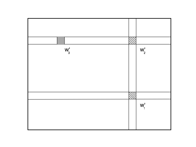
Figure 1: The three successive C–A steps output three striped matrices.

Sub-algorithm $\mathcal{B}$. This sub-algorithm verifies whether the error norm of the CUR LRA built on a fixed CUR generator is within a fixed tolerance $\tau$ (see [47] for some heuristic recipes for verification at sublinear cost).

1

Input: $W\in\mathbb{C}^{m\times n}$, four positive integers $r,k,l$, and ITER; a number $\tau>0$.

4 Output: A CUR LRA of $W$ with an error norm at most $\tau$ or FAILURE.

2  Initialization: Fix a submatrix $W_{0}$ made up of $l$ columns of $W$ and obtain an initial set $\mathcal{I}_{0}$.

3Computations:

  for $i=1,2,\dots,\textrm{ ITER}$ do

     if $i$ is even then

        ”Horizontal” C–A step:

        1. Let $R_{i}:=W_{\mathcal{I}_{i-1},:}$ be a $p\times n$ submatrix of $W$.

        2. Apply Sub-algorithm $\mathcal{A}$ for $q=n$ to $R_{i}$ and obtain a $k\times l$ submatrix $W_{i}=W_{\mathcal{I}_{i-1},\mathcal{J}_{i}}$.

     else

        ”Vertical” C–A step:

        1. Let $C_{i}:=W_{:,\mathcal{J}_{i-1}}$ be an $m\times q$ submatrix of $W$.

        2. Apply Sub-algorithm $\mathcal{A}$ for $p=m$ to $C_{i}$ and obtain a $k\times l$ submatrix $W_{i}=W_{\mathcal{I}_{i},\mathcal{J}_{i-1}}$.

     end if

     Apply Sub-algorithm $\mathcal{B}$ and obtain $E$, the error bound of CUR LRA built on the generator $W_{i}$.

     if $E\leq\tau$ then

        return  CUR LRA built on the generator $W_{i}$.

     end if

  end for

  return  Failure

Algorithm 1 C–A Iterations

PART II. CUR LRA FOR SPSD MATRICES

6 CUR LRA of SPSD Matrices: Main Results

We are going to devise an algorithm to which we refer as the Main Algorithm and Algorithm 5 and and which computes CUR LRA of an SPSD matrix at sublinear cost.

Theorem 6.1.

(Main Result 1) Suppose that $W\in\mathbb{R}^{n\times n}$ is an SPSD matrix, $r$ and $n$ are two positive integers, $r<n$, $\epsilon$ is a positive number, and $\mathcal{I}$ is the output of Algorithm 5 (Main Algorithm). Write $C:=W_{:,\mathcal{I}}$, $U:=W_{\mathcal{I},\mathcal{I}}^{-1}$, and $R:=W_{\mathcal{I},:}$. Then

$$||W-CUR||_{C}\leq(1+\epsilon)(r+1)\sigma_{r+1}(W).$$ (6.1)

Furthermore Algorithm 5 runs at an arithmetic cost in $O(nr^{4}\epsilon^{-1}\log r)$ as $\epsilon\rightarrow 0$.

Theorem 6.2.

(Main Result 2) Suppose that $W\in\mathbb{R}^{n\times n}$ is an SPSD matrix, $r$, $K$ and $n$ are three positive integers such that $r<K<n$, $\epsilon$ is a a positive number, and $\mathcal{I}$ is the output of Algorithm 5 (Main Algorithm). Write $C:=W_{:,\mathcal{I}}$, $U:=(W_{\mathcal{I},\mathcal{I}})_{r}^{+}$, and $R:=W_{\mathcal{I},:}$. Then

$$||W-CUR||_{C}\leq(1+\epsilon)\frac{K+1}{K-r+1}\sigma_{r+1}(W).$$ (6.2)

In particular, let $K=cr-1$ for $c>1$. Then

$$||W-CUR||_{C}\leq(1+\frac{1}{c-1})(1+\epsilon)\sigma_{r+1}(W).$$ (6.3)

Furthermore Algorithm 5 runs at an arithmetic cost in $O((r+\log n)rK^{4}n\epsilon^{-1})$ as $\epsilon\rightarrow 0$.

7 Proof of Main Result 1

Hereafter $[n]$ denotes the set $\{1,2,\dots,n\}$ of $n$ integers $1,2,\dots,n$.

$\mathcal{I}\subset[n]$ denotes a set of indices, while $|\mathcal{I}|$ denotes the cardinality (the number of elements) of $\mathcal{I}$.

1

Input: $A\in\mathbb{R}^{m\times n}$ and a positive integer $K<n$.

2 Output: $\mathcal{I}$.

  Initialize $\mathcal{I}=\{\}$.

  $M^{1}\leftarrow A$.

  for t = 1, 2, …, K do

     $i\leftarrow\operatorname*{arg\,max}_{a\in[n]}||M^{t}_{:,a}||$

     $\mathcal{I}\leftarrow\mathcal{I}\cup\{i\}$.

     $M^{t+1}\leftarrow M^{t}-||M^{t}_{:,i}||^{-2}(M^{t}_{:,i})(M^{t}_{:,i})^{T}M^{t}$

  end for

  return  $\mathcal{I}$.

Algorithm 2 Greedy Column Subset Selection [24].

Theorem 7.1 below enables us to decrease the cost of searching for the maximal volume submatrix an SPSD matrix by restricting the search to the principal submatrices. As pointed out in [22] and implicit in [24], the task is still NP hard and therefore is impractical for inputs of even moderately large size. [22] proposed to search for a submatrix with a large volume by means of a greedy algorithm that is essentially Gaussian Elimination with Complete Pivoting (Algorithm 3 GECP). This, however, only guarantees an error bound of $4^{r}~{}\sigma_{r+1}(W)$ in the Chebyshev norm for the output CUR LRA.

Theorem 7.1.

(Cf. [22].) Suppose that $W$ is an $n\times n$ SPSD matrix and $\mathcal{I}$ and $\mathcal{J}$ are two sets of integers in $[n]$ having the same cardinality. Then $\operatorname*{{\it v}_{2}}\left\lparen W_{\mathcal{I},\mathcal{J}}\right\rparen^{2}\leq\operatorname*{{\it v}_{2}}\left\lparen W_{\mathcal{I},\mathcal{I}}\right\rparen\operatorname*{{\it v}_{2}}\left\lparen W_{\mathcal{J},\mathcal{J}}\right\rparen.$

1

Input: An SPSD matrix $A\in\mathbb{R}^{n\times n}$ and a positive integer $K<n$.

Output: $\mathcal{I}$.

  Initialize $R\leftarrow A$, and $\mathcal{I}=\{\}$.

  for t = 1, 2, …, K do

     $i_{t}\leftarrow\operatorname*{arg\,max}_{j\in[n]}|R_{j,j}|$.

     $\mathcal{I}\leftarrow\mathcal{I}\cup\{i_{t}\}$.

     $R\leftarrow R-R_{:,i_{t}}\cdot r_{i_{t},i_{t}}^{-1}\cdot R_{i_{t},:}$.

  end for

  return  $\mathcal{I}$.

Algorithm 3 An SPSD Matrix: Gaussian Elimination with Complete Pivoting (cf. [22]).

The papers [35] and [57] enable us to simplify our task further by proving that if the generator $W_{\mathcal{I},\mathcal{I}}$ has $(1+\epsilon)$-locally maximal volume, then the CUR LRA generated by it has error bound $(1+\epsilon)(1+r)\sigma_{r+1}(W)$ in Chebyshev norm. This is a dramatic improvement over the error bound $4^{r}~{}\sigma_{r+1}(W)$ of [22]. For a general input matrix, finding a submatrix with locally maximal volume or even verifying this property is still quite costly, because one would potentially need to compare the volumes of order of $n^{2}$ “nearby” submatrices, where we say that two matrices are nearby matrices if they differ at most by a single row and/or column. In the case of an SPSD input we combine the results of [35] and [57] with Theorem 7.1, and then these combined results enable us to verify that a principal submatrix has maximal or nearly maximal volume by comparing its volume with that of its $O(n)$ “nearby” principal submatrices. We state this observation formally in the following Theorem 7.2.

Theorem 7.2.

Suppose that $W\in\mathbb{R}^{n\times n}$ is an SPSD matrix, $\mathcal{I}$ is an index set, and $0<|\mathcal{I}|=r<n$. Let $(1+\epsilon)\cdot\operatorname*{{\it v}_{2}}\left\lparen W_{\mathcal{I},\mathcal{I}}\right\rparen\geq\operatorname*{{\it v}_{2}}\left\lparen W_{\mathcal{J},\mathcal{J}}\right\rparen$ for any index set $\mathcal{J}$ where $|\mathcal{J}|=r$, and $\mathcal{J}$ only differs from $\mathcal{I}$ at a single element. Then $W_{\mathcal{I},\mathcal{I}}$ is a $(1+\epsilon)$-locally maximal volume submatrix.

Proof.

Let $\mathcal{I}^{\prime}$ and $\mathcal{J}^{\prime}$ be any two index sets where $|\mathcal{I}^{\prime}|=|\mathcal{J}^{\prime}|=r$, and let them differ from $\mathcal{I}$ at most at a single element. Apply [22, Thm. 1] and obtain that $\operatorname*{{\it v}_{2}}\left\lparen W_{\mathcal{I}^{\prime},\mathcal{J}^{\prime}}\right\rparen\leq\max\big{(}\operatorname*{{\it v}_{2}}\left\lparen W_{\mathcal{I}^{\prime},\mathcal{I}^{\prime}}\right\rparen,\operatorname*{{\it v}_{2}}\left\lparen W_{\mathcal{J}^{\prime},\mathcal{J}^{\prime}}\right\rparen\big{)}\leq(1+\epsilon)\cdot\operatorname*{{\it v}_{2}}\left\lparen W_{\mathcal{I},\mathcal{I}}\right\rparen$. The latter inequality follows from the assumption. ∎

Given an index set $\mathcal{I}_{0}$, with $|\mathcal{I}_{0}|=r$, and a positive number $\epsilon$, Algorithm 4 (Index Update) finds whether there is a “nearby” principal submatrices of $W_{\mathcal{I}_{0},\mathcal{I}_{0}}$ whose volume is at least $(1+\epsilon)\cdot\operatorname*{{\it v}_{2}}\left\lparen W_{\mathcal{I}_{0},\mathcal{I}_{0}}\right\rparen$, and if there is one, then updates the index set $\mathcal{I}_{0}$ accordingly. Therefore if we recursively apply this algorithm until no index update is possible, then the final index set $\mathcal{I}$ determines an $r\times r$ submatrix that has locally $(1+\epsilon)$-maximal volume; in this case the error bound of Main Result 1 can be readily deduced from Theorem 4.1.

Having proved correctness of Algorithm 5 (Main Algorithm), we still need to estimate its complexity. We only need to find (i) a good initial index set $\mathcal{I}_{0}$ efficiently and (ii) a submatrix having $(1+\epsilon)$-locally maximal volume. We achieve this in a relatively small number of recursive applications of Algorithm 4 (Index Update).

We first show that Algorithm 3 (GECP) runs efficiently and determines a submatrix having a relatively large volume. For a general input matrix, the pivoting stage of GECP is especially costly because the element with the greatest modulus could appear anywhere in the residual matrix. For SPSD matrices, however, the residual is also SPSD; therefore we only need to examine such elements on the diagonal.

Next we show that the initial principal submatrix found by Algorithm 3 (GECP) has a substantial volume.

Theorem 7.3.

(Adapted from [24, Thm. 10].) Suppose that Algorithm 2 has been applied to an input matrix $C\in\mathbb{R}^{m\times n}$ and an integer $r$ from the set $[n]$ and that it has output a set $\mathcal{I}$. Then

$$\operatorname*{{\it v}_{2}}\left\lparen C_{:,\mathcal{I}}\right\rparen\geq\frac{1}{r!}\max_{\mathcal{S}\subset[n]:|\mathcal{S}|=r}\operatorname*{{\it v}_{2}}\left\lparen C_{:,\mathcal{S}}\right\rparen.$$ (7.1)

Theorem 7.4.

For an SPSD matrix $W\in\mathbb{R}^{n\times n}$ and a positive integer $r<n$, let $\mathcal{I}$ be the output of Algorithm 3 (GECP) with inputs $W$ and $r$. Then

$$\operatorname*{{\it v}_{2}}\left\lparen W_{\mathcal{I},\mathcal{I}}\right\rparen\geq\frac{1}{(r!)^{2}}\max_{\mathcal{S}\subset[n]:|\mathcal{S}|=r}\operatorname*{{\it v}_{2}}\left\lparen W_{\mathcal{S},\mathcal{S}}\right\rparen.$$ (7.2)

Proof.

Since $W$ is SPSD, there exists $C\in\mathbb{R}^{n\times n}$ such that $W=C^{T}C$. Therefore, for any non-empty index set $\mathcal{J}\subset[n]$,

$$W_{\mathcal{J},\mathcal{J}}=C_{:,\mathcal{J}}^{T}C_{:,\mathcal{J}},$$ (7.3)

and thus

$$\operatorname*{{\it v}_{2}}\left\lparen W_{\mathcal{J},\mathcal{J}}\right\rparen=\big{(}\operatorname*{{\it v}_{2}}\left\lparen C_{:,\mathcal{J}}\right\rparen\big{)}^{2}.$$ (7.4)

Let us run Algorithm 2 (Greedy Column Subset Selection) and Algorithm 3 (GECP) with inputs ($C$, $k$) and ($W$, $k$), respectively, and let $\mathcal{I}$ and $\mathcal{I}^{\prime}$ be the outputs, respectively. Since both algorithms use greedy approach, we have

$$\operatorname*{{\it v}_{2}}\left\lparen W_{\mathcal{I},\mathcal{I}}\right\rparen =\big{(}\operatorname*{{\it v}_{2}}\left\lparen C_{:,\mathcal{I}^{\prime}}\right\rparen\big{)}^{2}$$ (7.5)

$$\geq\frac{1}{(r!)^{2}}\max_{\mathcal{S}\subset[n]:|\mathcal{S}|=r}\operatorname*{{\it v}_{2}}\left\lparen C_{:,\mathcal{S}}\right\rparen^{2}$$ (7.6)

$$=\frac{1}{(r!)^{2}}\max_{\mathcal{S}\subset[n]:|\mathcal{S}|=r}\operatorname*{{\it v}_{2}}\left\lparen W_{\mathcal{S},\mathcal{S}}\right\rparen.$$ (7.7)

∎

Let $\mathcal{I}_{0}$ be the initial index set obtained from Algorithm 3 (GECP), and let $\mathcal{I}_{1},\mathcal{I}_{2},\dots$ be the index sets that we obtained by recursively applying Algorithm 4 (Index Update). If we let $\epsilon>0$, then the volumes of the corresponding submatrices are strictly increasing, and therefore their sequence becomes invariant starting with some integer $T$. Furthermore, $\operatorname*{{\it v}_{2}}\left\lparen W_{\mathcal{I}_{t},\mathcal{I}_{t}}\right\rparen/\operatorname*{{\it v}_{2}}\left\lparen W_{\mathcal{I}_{0},\mathcal{I}_{0}}\right\rparen\geq(1+\epsilon)^{t}$ for $t\leq T$, and therefore $T\leq\log_{1+\epsilon}(r!)$. Recall that $\log_{1+\epsilon}(a)=\frac{\log(a)}{\log(1+\epsilon)}=O(\frac{\log(a)}{\epsilon})$as $\epsilon\rightarrow 0$, for all positive $a$. For $a=r!$ this turns into equation $\log_{1+\epsilon}(r!)=O(r\epsilon^{-1}\log r)$ as $\epsilon\rightarrow 0$, and we arrive at the following result.

Corollary 7.1.

For an SPSD matrix $W\in\mathbb{R}^{n\times n}$ and an integer $r$ in the set $[n-1]$, Algorithm 5 (Main Algorithm) calls Algorithm 4 (Index Update) $O(r\epsilon^{-1}\log r)$ times as $\epsilon\rightarrow 0$.

1

Input: An SPSD matrix $A\in\mathbb{R}^{n\times n}$, a set $\mathcal{I}\in[n]$, a positive integer $r\leq|\mathcal{I}|$, and a positive number $\epsilon$.

Output: $\mathcal{J}$

  Compute $\operatorname*{{\it v}_{2,r}}\big{(}A_{\mathcal{I},\mathcal{I}}\big{)}$

  for all $i\in\mathcal{I}$ do

     $\mathcal{I}^{\prime}\leftarrow\mathcal{I}-\{i\}$

     for all $j\in[n]-\mathcal{I}$  do

        $\mathcal{J}\leftarrow\mathcal{I}^{\prime}\cup\{j\}$

        Compute $\operatorname*{{\it v}_{2,r}}\big{(}A_{\mathcal{J},\mathcal{J}}\big{)}$

        if $\operatorname*{{\it v}_{2,r}}\big{(}A_{\mathcal{J},\mathcal{J}}\big{)}/\operatorname*{{\it v}_{2,r}}\big{(}A_{\mathcal{I},\mathcal{I}}\big{)}>1+\epsilon$ then

           return  $\mathcal{J}$

        end if

     end for

  end for

  return  $\mathcal{I}$

Algorithm 4 Index Update

1

Input: An SPSD matrix $A\in\mathbb{R}^{n\times n}$, two positive integers $K$ and $r$ such that $r\leq K<n$, and a positive number $\epsilon$. (We let $K=r$ if $K$ is not specified.)

Output: $\mathcal{I}$

  $\mathcal{I}\leftarrow$ Algorithm 3$(A,K)$

  while TRUE do

     $\mathcal{J}\leftarrow$ Algorithm 4$(A,\mathcal{I},r,\epsilon)$

     if $\mathcal{J}=\mathcal{I}$ then

        BREAK

     else

        $\mathcal{I}\leftarrow\mathcal{J}$

     end if

  end while

  return  $\mathcal{I}$.

Algorithm 5 Main Algorithm

8 Proof of Main Result 2

We begin with an auxiliary result.

Lemma 8.1.

Suppose that $W\in\mathbb{R}^{n\times n}$ is an SPSD matrix, $\mathcal{I}$ and $\mathcal{J}$ are two non-empty index sets, $|\mathcal{I}|=|\mathcal{J}|=K<n$, and $r\leq K$ is a positive integer. Then

$$\textstyle{\operatorname*{{\it v}_{2,r}}\big{(}W_{\mathcal{I},\mathcal{J}}\big{)}}\leq\max\Big{(}\textstyle{\operatorname*{{\it v}_{2,r}}\big{(}W_{\mathcal{I},\mathcal{I}}\big{)}},\textstyle{\operatorname*{{\it v}_{2,r}}\big{(}W_{\mathcal{J},\mathcal{J}}\big{)}}\Big{)}.$$ (8.1)

Proof.

Let $W=C^{T}C$ for some $C\in\mathbb{R}^{n\times n}$. Then

$$\textstyle\operatorname*{{\it v}_{2,r}}\big{(}W_{\mathcal{I},\mathcal{J}}\big{)} =\textstyle\operatorname*{{\it v}_{2,r}}\big{(}C_{:,\mathcal{I}}^{T}C_{:,\mathcal{J}}\big{)}$$ (8.2)

$$\leq\textstyle\operatorname*{{\it v}_{2,r}}\big{(}C_{:,\mathcal{I}}\big{)}\textstyle\operatorname*{{\it v}_{2,r}}\big{(}C_{:,\mathcal{J}}\big{)}$$ (8.3)

$$=\sqrt{\textstyle\operatorname*{{\it v}_{2,r}}\big{(}W_{\mathcal{I},\mathcal{I}}\big{)}\textstyle\operatorname*{{\it v}_{2,r}}\big{(}W_{\mathcal{J},\mathcal{J}}\big{)}}.$$ (8.4)

Inequality (8.3) follows from Theorem 4.4 (ii). ∎

Lemma 8.1 shows that, similarly to the case of matrix volume, the search for the maximal $r$-projective volume submatrix of an SPSD matrix can be restricted to its principal submatrices and that Theorem 7.2 can be extended to submatrices with locally maximal $r$-projective volume. Next we formally state these observations

Theorem 8.1.

Suppose that $W\in\mathbb{R}^{n\times n}$ is an SPSD matrix, $\epsilon$ is a positive number, $\mathcal{I}\subset[n]$ is an index set, $|\mathcal{I}|=K$, $r$ is an integer, $r<K<n$, and for all $\mathcal{J}\subset[n]$, where $|\mathcal{J}|=K$ and $\mathcal{J}$ differs from $\mathcal{I}$ at a single element, the inequality $(1+\epsilon)\cdot\operatorname*{{\it v}_{2,r}}\big{(}W_{\mathcal{I},\mathcal{I}}\big{)}\geq\operatorname*{{\it v}_{2,r}}\big{(}W_{\mathcal{J},\mathcal{J}}\big{)}$ holds. Then $W_{\mathcal{I},\mathcal{I}}$ has $(1+\epsilon)$-locally maximal $r$-projective volume.

Based on the above result and extending the argument of Section 7 we can show that Algorithm 5 (Main Algorithm) finds a principal submatrix with $(1+\epsilon)$-locally maximal $r$-projective volume. Together with the result of Theorem 4.2 this implies correctness of the error bound of Main Result 2, and we will bound the arithmetic cost next.

Let $T$ denote the number of invocations of Index Update required to arrive at a submatrix having $(1+\epsilon)$-locally maximal $r$-projective volume beginning from the initial principal submatrix obtained from Algorithm 3 (GECP). We deduce that Algorithm 5 (Main Algorithm) has sublinear complexity by proving that $T$ is sublinear in $n$. Recall the well-known bound on the volume of the greedily selected column submatrix from [30], and then the claim follows readily.

Lemma 8.2.

(Cf. [30, Thm. 7.2] and [24, Thm. 10].) Suppose that $C\in\mathbb{R}^{m\times n}$, $r$ and $K$ are integers, $0<r\leq K<n$, and $\mathcal{I}$ is the output of Algorithm 2 (Greedy Column Subset Selection) with input $C$ and $K$. Then

$$\textstyle\operatorname*{{\it v}_{2,r}}\big{(}C_{:,\mathcal{I}}\big{)}\geq 2^{-r(r-1)/2}n^{-r/2}\textstyle\operatorname*{{\it v}_{2,r}}\big{(}C\big{)}$$ (8.5)

Theorem 7.4 implies that $\operatorname*{{\it v}_{2,r}}(W)/\operatorname*{{\it v}_{2,r}}(W_{\mathcal{I},\mathcal{I}})\geq 2^{r(r-1)}n^{r}$, where $\mathcal{I}$ is the initial index set obtained by Algorithm 3 (GECP). Recall that $\operatorname*{{\it v}_{2,r}}(W)$ is the $r$-projective volume upper bound for any submatrix of $W$, and therefore the number $T$ of required Index Updates is bounded by $\log_{1+\epsilon}(2^{r(r-1)}n^{r})=O(r^{2}\epsilon^{-1}+\epsilon^{-1}r\log n)$.

9 Complexity Analysis

In this section, we estimate the time complexity of performing the Main Algorithm (Algorithm 5) separately in two cases where $r=K$ and $r<K$.

The cost of computing the initial set $\mathcal{I}_{0}$ by means of Algorithm 3 (GECP) is $O(nK^{2})$. Let $t$ denote the number of iterations and let $c(r,K)$ denote the arithmetic cost of performing Algorithm 4 (Index Update) with parameters $r$ and $K$. Then the complexity is in $O(nK^{2}+t\cdot c(r,K))$.

In the case where $r=K$, Corollary 7.1 implies that $t=O(r\epsilon^{-1}\log r)$. Algorithm 4 (Index Update) needs up to $nr$ comparisons of $\operatorname*{{\it v}_{2}}\big{(}W_{\mathcal{I},\mathcal{I}}\big{)}$ and $\operatorname*{{\it v}_{2}}\big{(}W_{\mathcal{J},\mathcal{J}}\big{)}$. Since $\mathcal{I}$ and $\mathcal{J}$ differs by at most at one index, we compute $\operatorname*{{\it v}_{2}}\big{(}W_{\mathcal{J},\mathcal{J}}\big{)}$ faster by using small rank update of $\operatorname*{{\it v}_{2}}\big{(}W_{\mathcal{I},\mathcal{I}})$ instead of computing from the scratch; this saves a factor of $k$. Therefore $c(r,r)=O(r^{3}n)$, and the time complexity of the Main Algorithm is in $O(nr^{4}\epsilon^{-1}\log r)$.

Finally let $r<K$. Then according to [30, Theorem 7.2] and [24, Theorem 10], $t$ increases slightly – staying in $O(r^{2}\epsilon^{-1}+\epsilon^{-1}r\log n)$; if $\operatorname*{{\it v}_{2,r}}\big{(}W_{\mathcal{J},\mathcal{J}}\big{)}$ is computed by using SVD, then $c(r,K)=O(K^{4}n)$, and the time complexity of the Main Algorithm is in $O((r+\log n)rK^{4}n\epsilon^{-1})$.

PART III. CUR LRA BY MEANS OF C-A ITERATIONS

10 Overview

In the next section we show that already two successive C-A iterations output a CUR generator having $h$-maximal volume (for any $h>1$) if these iterations begin at a $p\times q$ submatrix of $W$ that shares its rank $r>0$ with $W$. By continuity of the volume the result is extended to perturbations of such matrices within a norm bound estimated in Theorem 4.3. In Section 12 we extend these results to the case where $r$-projective volume rather than the volume of a CUR generator is maximized; Theorem 4.2 shows benefits of such a maximization. In Section 13 we estimate the complexity and accuracy of a two-step loop of C–A iterations. In Sections 14 and 15 we demonstrate the power of C-A iterations by means of the acceleration of the FMM method to superfast level, that is, to performing it at sublinear cost.

11 Volume of the Output of a C–A loop

We can apply C–A steps by choosing deterministic algorithms of [30] for Sub-algorithm $\mathcal{A}$. In this case $mq$ and $pn$ memory cells and $O(mq^{2})$ and $O(p^{2}n)$ arithmetic operations are involved in “vertical” and “horizontal” C-A iterations, respectively. They run at sublinear cost if $p^{2}=o(m)$ and $q^{2}=o(n)$ and output submatrices having $h$-maximal volumes for $h$ being a low degree polynomial in $m+n$. Every iteration outputs a matrix that has locally $h$-maximal volume in a “vertical” or “horizontal” submatrix, and we hope to obtain globally $\bar{h}$-maximal submatrix (for reasonably bounded $\bar{h}$) when maximization is performed recursively in alternate directions.

We readily prove that this expectation is true for a low rank input matrix and hence, by virtue of Theorem 4.3, for a matrix that admits its sufficiently close LRA. The error bound of the LRA deviates from optimal by the factor $\bar{h}$ even in Chebyshev norm, but in spite of this deficiency (see some remedy at the end of Section 1.1) and a strong restriction on the input class, we still yield some limited formal support for the long-known empirical efficiency of C-A iterations.

Let us next elaborate upon this support.

By comparing SVDs of the matrices $W$ and $W^{+}$ obtain the following lemma.

Lemma 11.1.

$\sigma_{j}(W)\sigma_{\operatorname{rank}(W)+1-j}(W^{+})=1$ for all matrices $W$ and all integers $j$ not exceeding $\operatorname{rank}(W)$.

Corollary 11.1.

$v_{2}(W)v_{2}(W^{+})=1$ and $v_{2,r}(W)v_{2,r}(W_{r}^{+})=1$ for all matrices $W$ of full rank and all integers $r$ such that $1\leq r\leq\operatorname{rank}(W)$.

We are ready to prove that a $k\times l$ submatrix of rank $r$ has $hh^{\prime}$-maximal volume globally in a rank-$r$ matrix $W$, that is, over all $k\times l$ submatrices of $W$, if it has $(h,h^{\prime})$ maximal nonzero volume in this matrix $W$.

Theorem 11.1.

Suppose that the volume of a $k\times l$ submatrix $W_{\mathcal{I},\mathcal{J}}$ is nonzero and $(h,h^{\prime})$-maximal in a matrix $W$ for $h\geq 1$ and $h^{\prime}\geq 1$ where $\operatorname{rank}(W)=r=\min\{k,l\}$. Then this volume is $hh^{\prime}$-maximal over all its $k\times l$ submatrices of the matrix $W$.

Proof.

The matrix $W_{\mathcal{I},\mathcal{J}}$ has full rank because its volume is nonzero.

Fix any $k\times l$ submatrix $W_{\mathcal{I}^{\prime},\mathcal{J}^{\prime}}$ of the matrix $W$, recall that $W=CUR$, and obtain that

$$W_{\mathcal{I}^{\prime},\mathcal{J}^{\prime}}=W_{\mathcal{I}^{\prime},\mathcal{J}}W_{\mathcal{I},\mathcal{J}}^{+}W_{\mathcal{I},\mathcal{J}^{\prime}}.$$

If $k\leq l$, then first apply claim (iii) of Theorem 4.4 for $G:=W_{\mathcal{I}^{\prime},\mathcal{J}}$ and $H:=W_{\mathcal{I},\mathcal{J}}^{+}$; then apply claim (i) of that theorem for $G:=W_{\mathcal{I}^{\prime},\mathcal{J}}W_{\mathcal{I},\mathcal{J}}^{+}$ and $H:=W_{\mathcal{I},\mathcal{J}^{\prime}}$ and obtain that

$$v_{2}(W_{\mathcal{I}^{\prime},\mathcal{J}})=v_{2}(W_{\mathcal{I}^{\prime},\mathcal{J}}W_{\mathcal{I},\mathcal{J}}^{+}W_{\mathcal{I},\mathcal{J}^{\prime}})\leq v_{2}(W_{\mathcal{I}^{\prime},\mathcal{J}})v_{2}(W_{\mathcal{I},\mathcal{J}}^{+})v_{2}(W_{\mathcal{I},\mathcal{J}^{\prime}}).$$

If $k>l$ deduce the same bound by applying the same argument to the matrix equation

$$W_{\mathcal{I}^{\prime},\mathcal{J}^{\prime}}^{T}=W_{\mathcal{I},\mathcal{J}^{\prime}}^{T}W_{\mathcal{I},\mathcal{J}}^{+T}W_{\mathcal{I}^{\prime},\mathcal{J}}^{T}.$$

Combine this bound with Corollary 11.1 for $W$ replaced by $W_{\mathcal{I},\mathcal{J}}$ and deduce that

$$v_{2}(W_{\mathcal{I}^{\prime},\mathcal{J}^{\prime}})=v_{2}(W_{\mathcal{I}^{\prime},\mathcal{J}}W_{\mathcal{I},\mathcal{J}}^{+}W_{\mathcal{I},\mathcal{J}^{\prime}})\leq v_{2}(W_{\mathcal{I}^{\prime},\mathcal{J}})v_{2}(W_{\mathcal{I},\mathcal{J}^{\prime}})/v_{2}(W_{\mathcal{I},\mathcal{J}}).$$ (11.1)

Recall that the matrix $W_{\mathcal{I},\mathcal{J}}$ is $(h,h^{\prime})$-maximal and conclude that

$$hv_{2}(W_{\mathcal{I},\mathcal{J}})\geq v_{2}(W_{\mathcal{I},\mathcal{J}^{\prime}})~{}{\rm and}~{}h^{\prime}v_{2}(W_{\mathcal{I},\mathcal{J}})\geq v_{2}(W_{\mathcal{I}^{\prime},\mathcal{J}}).$$

Substitute these inequalities into the above bound on the volume $v_{2}(W_{\mathcal{I}^{\prime},\mathcal{J}^{\prime}})$ and obtain that $v_{2}(W_{\mathcal{I}^{\prime},\mathcal{J}^{\prime}})\leq hh^{\prime}v_{2}(W_{\mathcal{I},\mathcal{J}})$. ∎

12 From the Maximal Volume to the Maximal $r$-Projective Volume

Recall that the CUR LRA error bound of Theorem 4.1 is strengthened when we shift to Theorem 4.2, that is, maximize $r$-projective volume for $r<k=l$ rather than the volume. Next we reduce maximization of $r$-projective volume of a CUR generators to volume maximization.

Recall that multiplication by a square orthogonal matrix changes neither the volume nor $r$-projective volume of a matrix and obtain the following result.

Lemma 12.1.

Let $M$ and $N$ be a pair of $k\times l$ submatrices of a $k\times n$ matrix and let $Q$ be a $k\times k$ orthogonal matrix. Then $v_{2}(M)/v_{2}(N)=v_{2}(QM)/v_{2}(QN)$, and if $r\leq\min\{k,l\}$ then also $v_{2,r}(M)/v_{2,r}(N)=v_{2,r}(QM)/v_{2,r}(QN)$.

1

Input: Four integers $k,l,n,$ and $r$ such that $0<r\leq k\leq n$ and $r\leq l\leq n$; a $k\times n$ matrix $W$ of rank $r$; a black box algorithm that finds an $r\times l$ submatrix having locally maximal volume in an $r\times n$ matrix of full rank $r$.

2 Output: A column set $\mathcal{J}$ such that $W_{:,\mathcal{J}}$ has maximal $r$-projective volume in $W$.

Computations:

  1. Compute a rank-revealing QRP factorization $W=QRP$, where $Q$ is an orthogonal matrix, $P$ is a permutation matrix, $R=\begin{pmatrix}R^{\prime}\\ O\end{pmatrix}$, and $R^{\prime}$ is an $r\times n$ matrix. (See [32, Sections 5.4.3 and 5.4.4] and [30].)

  2. Compute an $r\times l$ submatrix $R^{\prime}_{:,\mathcal{J}}$ of $R^{\prime}$ having maximal volume.

  return  $\mathcal{J}^{\prime}$ such that $P:\mathcal{J}^{\prime}\longrightarrow\mathcal{J}$.

Algorithm 6 From maximal volume to maximal $r$-projective volume

The submatrices $R^{\prime}$ and $\begin{pmatrix}R^{\prime}\\ O\end{pmatrix}$ of the matrix $R$ of Algorithm 6 have maximal volume and maximal $r$-projective volume in the matrix $R$, respectively, by virtue of Theorem 4.4 and because $v_{2}(R)=v_{2,r}(R)=v_{2,r}(R^{\prime})$. Therefore the submatrix $W_{:,\mathcal{J}}$ has maximal $r$-projective volume in the matrix $W$ by virtue of Lemma 12.1.

Remark 12.1.

By transposing a horizontal input matrix $W$ and interchanging the integers $m$ and $n$ and the integers $k$ and $l$ we extend the algorithm to computing a $k\times l$ submatrix of maximal or nearly maximal $r$-projective volume in an $m\times l$ matrix of rank $r$.

13 Complexity and Accuracy of an C–A Loop

The following theorem summarizes our study in this part of the paper.

Theorem 13.1.

Given five integers $k$, $l$, $m$, $n$, and $r$ such that $0<r\leq k\leq m$ and $r\leq l\leq n$, suppose that two successive C–A steps (say, based on the algorithms of [30]) combined with Algorithm 6 have been applied to an $m\times n$ matrix $W$ of rank $r$ and have output a pair of $k\times l$ submatrices $W^{\prime}_{1}$ and $W^{\prime}_{2}=W_{\mathcal{I}_{2},\mathcal{J}_{2}}$ with nonzero $r$-projective column-wise locally $h$-maximal and nonzero $r$-projective row-wise locally $h^{\prime}$-maximal volumes, respectively. Then the submatrix $W_{2}^{\prime}$ has $h^{\prime}h$-maximal $r$-projective volume in the matrix $W$.

By combining Theorems 4.1, 4.2, and 13.1 we obtain the following corollary.

Corollary 13.1.

Under the assumptions of Theorem 13.1 apply a two-step C–A loop to an $m\times n$ matrix $W$ of rank $r$ and suppose that both its C–A steps output $k\times l$ submatrices having nonzero $r$-projective column-wise and row-wise locally $h$-maximal volumes (see Remark 13.1 below). Build a canonical CUR LRA on a CUR generator $W_{2}^{\prime}=W_{k,l}$ of rank $r$ output by the second C–A step. Then

(i) the computation of this CUR LRA by using the auxiliary algorithms of [30] involves $(m+n)r$ memory cells and $O((m+n)r^{2})$ arithmetic operations and

(ii) the error matrix $E$ of the output CUR LRA satisfies the bound $||E||_{C}\leq g(k,l,r)~{}\bar{h}~{}\sigma_{r+1}(W)$ for $\bar{h}$ of Theorem 13.1 and $g(k,l,r)$ denoting the functions $f(k,l)$ of Theorem 4.1 or $f(k,l,r)$ of Theorem 4.2. In particular $||E||_{C}\leq 2hh^{\prime}\sigma_{2}(W)$ for $k=l=r=1$.

Remark 13.1.

Theorem 4.3 enables us to extend Theorem 13.1 and Corollary 13.1 to the case of an input matrix $W$ of numerical rank $r$ as long as a C-A step begins with a non-degenerating input matrix sharing its numerical rank $r$ with an input matrix $W$.

14 Superfast Multipole Method

Sublinear cost LRA algorithms can be extended to numerous important computational problems linked to LRA. Next we point out and extensively test a simple application to the acceleration of the celebrated Fast Multipole Method (FMM) (cf. [34], [17], [26], [16], [14], and the bibliography therein), which turns it into Superfast Multipole Method.

FMM enables multiplication by a vector of so called HSS matrices at sublinear cost provided that low rank generators are available for its off-diagonal blocks. Such generators can be a part of the input, and it is frequently not emphasized that they are not available in a variety of other important applications of FMM (see, e.g., [84], [83], [61]). Even in such cases, however, by applying ACA algorithms of [1], [3] or the MaxVol algorithm of [33] we can compute the generators at sublinear cost, thus turning FMM into Superfast Multipole Method. Next we supply some details.

HSS matrices naturally extend the class of banded matrices and their inverses, are closely linked to FMM, and are increasingly popular. See [7], [31], [53], [18], [75], [76], [2], [81], [84], [28], [82], [83], the references therein, software libraries H2Lib, http://www.h2lib.org/, https://github.com/H2Lib/H2Lib, and HLib, www.hlib.org, developed at the Max Planck Institute for Mathematics in the Sciences.

Definition 14.1.

(Neutered Block Columns. See [53].) With each diagonal block of a block matrix associate its complement in its block column, and call this complement a neutered block column.

Definition 14.2.

(HSS matrices. See [18], [81], [82], [83].)

A block matrix $M$ of size $m\times n$ is called an $r$-HSS matrix, for a positive integer $r$,

(i) if all diagonal blocks of this matrix consist of $O((m+n)r)$ entries overall and

(ii) if $r$ is the maximal rank of its neutered block columns.

Remark 14.1.

Many authors work with $(l,u)$-HSS (rather than $r$-HSS) matrices $M$ for which $l$ and $u$ are the maximal ranks of the sub- and super-diagonal blocks, respectively. The $(l,u)$-HSS and $r$-HSS matrices are closely related. If a neutered block column $N$ is the union of a sub-diagonal block $B_{-}$ and a super-diagonal block $B_{+}$, then $\operatorname{rank}(N)\leq\operatorname{rank}(B_{-})+\operatorname{rank}(B_{+})$, and so an $(l,u)$-HSS matrix is an $r$-HSS matrix, for $r\leq l+u$, while clearly an $r$-HSS matrix is a $(r,r)$-HSS matrix.

The FMM exploits the $r$-HSS structure of a matrix as follows:

(i) Cover all off-block-diagonal entries with a set of non-overlapping neutered block columns.

(ii) Express every neutered block column $N$ of this set as the product $FH$ of two generator matrices, $F$ of size $h\times r$ and $H$ of size $r\times k$. Call the pair $\{F,H\}$ a length $r$ generator of the neutered block column $N$.

(iii) Multiply the matrix $M$ by a vector by separately multiplying generators and diagonal blocks by subvectors, involving $O((m+n)r)$ flops overall, and

(iv) in a more advanced application of FMM solve a nonsingular $r$-HSS linear system of $n$ equations by using $O(nr\log^{2}(n))$ flops under some mild additional assumptions on the input.

This approach is readily extended to the same operations with $(r,\xi)$-HSS matrices, that is, matrices approximated by $r$-HSS matrices within a perturbation norm bound $\xi$ where a positive tolerance $\xi$ is small in context (for example, is the unit round-off). Likewise, one defines an $(r,\xi)$-HSS representation and $(r,\xi)$-generators.

$(r,\xi)$-HSS matrices (for $r$ small in context) appear routinely in matrix computations, and computations with such matrices are performed efficiently by using the above techniques.

As we said already, in some applications of the FMM (see [10] and [77]) stage (ii) is omitted because short generators for all neutered block columns are readily available, but this is not the case in some other important applications. This stage of the computation of generators is precisely LRA of the neutered block columns; it turns out to be the bottleneck stage of FMM in these applications, and sublinear cost LRA algorithms provide a remedy.

First suppose that a known LRA algorithm, e.g., the algorithm of [41] with a Gaussian multiplier, is applied at this stage. Multiplication of a $q\times h$ matrix by an $h\times r$ Gaussian matrix requires $(2h-1)qr$ flops, while standard HSS-representation of an $n\times n$ HSS matrix includes $q\times h$ neutered block columns for $q\approx m/2$ and $h\approx n/2$. In this case the cost of computing an $r$-HSS representation of the matrix $M$ has at least order $mnr$. For $r\ll\min\{m,n\}$, this is much greater than $O((m+n)r\log^{2}(n))$ flops, used at the other stages of the computations. We, however, readily match the latter bound at the stage of computing $(r,\xi)$-generators as well – simply by applying sublinear cost LRA algorithms.

15 Computation of LRAs for Benchmark HSS Matrices

In this section we cover our tests of the Superfast Multipole Method where we applied C–A iterations in order to compute LRA of the generators of the off-diagonal blocks of HSS matrices. Namely we tested HSS matrices that approximate $1024\times 1024$ Cauchy-like matrices derived from benchmark Toeplitz matrices B, C, D, E, and F of [84, Section 5]. For the computation of LRA we applied the algorithm of [33].

Table 1 displays the relative errors of the approximation of the $1024\times 1024$ HSS input matrices in the spectral and +shev norms averaged over 100 tests. Each approximation was obtained by means of combining the exact diagonal blocks and LRA of the off-diagonal blocks. We computed LRA of all these blocks superfast.

In good accordance with extensive empirical evidence about the power of C–A iterations, already the first C–A loop has consistently output reasonably close LRA, but our further improvement was achieved in five C–A loops in our tests for all but one of the five families of input matrices.

The reported HSS rank is the larger of the numerical ranks for the $512\times 512$ off-diagonal blocks. This HSS rank was used as an upper bound in our binary search that determined the numerical rank of each off-diagonal block for the purpose of computing its LRA. We based the binary search on minimizing the difference (in the spectral norm) between each off-diagonal block and its LRA.

The output error norms were quite low. Even in the case of the matrix C, obtained from Prolate Toeplitz matrices – extremely ill-conditioned, they ranged from $10^{-3}$ to $10^{-6}$.

We have also performed further numerical experiments on all the HSS input matrices by using a hybrid LRA algorithm: we used random pre-processing with Gaussian and Hadamard (abridged and permuted) multipliers (cf. [64]) by incorporating them into Algorithm 4.1 of [41], but applying it only to the off-diagonal blocks of smaller sizes while retaining our previous way for computing LRA of the larger off-diagonal blocks. We have not displayed the results of these experiments because they yielded no substantial improvement in accuracy in comparison to the exclusive use of the less expensive LRA on all off-diagonal blocks.

			Spectral Norm		Chebyshev Norm
Inputs	C–A loops	HSS rank	mean	std	mean	std
B B	1	26	8.11e-07	1.45e-06	3.19e-07	5.23e-07
	5	26	4.60e-08	6.43e-08	7.33e-09	1.22e-08
C	1	16	5.62e-03	8.99e-03	3.00e-03	4.37e-03
	5	16	3.37e-05	1.78e-05	8.77e-06	1.01e-05
D	1	13	1.12e-07	8.99e-08	1.35e-07	1.47e-07
	5	13	1.50e-07	1.82e-07	2.09e-07	2.29e-07
E	1	14	5.35e-04	6.14e-04	2.90e-04	3.51e-04
	5	14	1.90e-05	1.04e-05	5.49e-06	4.79e-06
F	1	37	1.14e-05	4.49e-05	6.02e-06	2.16e-05
	5	37	4.92e-07	8.19e-07	1.12e-07	2.60e-07

Table 15.1: LRA approximation of HSS matrices from [84]

Appendix: Small families of hard inputs for sublinear LRA

Any sublinear cost LRA algorithm fails on the following small input families.

Example. Define a family of $m\times n$ matrices of rank 1 (we call them $\delta$-matrices):

$$\{\Delta_{i,j},~{}{i=1,\dots,m;~{}j=1,\dots,n}\}.$$

Also include the $m\times n$ null matrix $O_{m,n}$ into this family. Now fix any sublinear cost algorithm; it does not access the $(i,j)$th entry of its input matrices for some pair of $i$ and $j$. Therefore it outputs the same approximation of the matrices $\Delta_{i,j}$ and $O_{m,n}$, with an undetected error at least 1/2. Apply the same argument to the set of $mn+1$ small-norm perturbations of the matrices of the above family and to the $mn+1$ sums of the latter matrices with any fixed $m\times n$ matrix of low rank. Finally, the same argument shows that a posteriori estimation of the output errors of an LRA algorithm applied to the same input families cannot run at sublinear cost.

This example actually covers randomized LRA algorithms as well. Indeed suppose that with a positive constant probability an LRA algorithm does not access $K$ entries of an input matrix and apply this algorithm to two matrices of low rank whose difference at all these entries is equal to a large constant $C$. Then, clearly, with a positive constant probability the algorithm has errors at least $\frac{C}{2}$ at at least $\frac{K}{2}$ of these entries.

Acknowledgements: Our research has been supported by NSF Grants CCF–1116736, CCF–1563942, CCF–133834 and PSC CUNY Awards 62797-00-50 and 63677-00-51. We also thank A. Cortinovis, A. Osinsky, N. L. Zamarashkin for pointers to their papers [22] and [57], S. A. Goreinov for sending reprints of his papers, and E. E. Tyrtyshnikov for pointers to the bibliography and the challenge of formally supporting empirical power of C–A algorithms.

References

- [1] M. Bebendorf, Approximation of Boundary Element Matrices, Numer. Math., 86, 4, 565–589, 2000.
- [2] S. Börm, Efficient Numerical Methods for Non-local Operators: -Matrix Compression, Algorithms and Analysis, European Math. Society, 2010.
- [3] M. Bebendorf, Adaptive Cross Approximation of Multivariate Functions, Constructive approximation, 34, 2, 149–179, 2011.
- [4] Elvar K. Bjarkason, Pass-Efficient Randomized Algorithms for Low-Rank Matrix Approximation Using Any Number of Views, SIAM Journal on Scientific Computing 41(4) A2355 - A2383 7 (2019), preprint in arXiv:1804.07531 (2018)
- [5] A. Ben-Israel, A Volume Associated with Matrices, Linear Algebra and its Applications, 167, 87–111, 1992.
- [6] A. Bakshi, N. Chepurko, D. P. Woodruff, Robust and Sample Optimal Algorithms for PSD Low-Rank Approximation, Proc. IEEE FOCS (2020).
- [7] S. Börm, L. Grasedyck, W. Hackbusch, Introduction to Hierarchical Matrices with Applications, Engineering Analysis with Boundary Elements, 27, 5, 405–422, 2003.
- [8] P.A. Businger, G. H. Golub, Linear Least Squares Solutions by Householder Transformations, Numer. Math., 7, 269–276, 1965.
- [9] M. Bebendorf, R. Grzhibovskis, Accelerating Galerkin BEM for linear elasticity using adaptive cross approximation, Math. Methods Appl. Sci., 29, 1721–1747, 2006.
- [10] A. Bini, L. Gemignani, V. Y. Pan, Fast and Stable QR Eigenvalue Algorithms for Generalized Semiseparable Matrices and Secular Equation, Numerische Mathematik, 100, 3, 373–408, 2005.
- [11] D. A. Bini, V. Y. Pan, Polynomial and Matrix Computations, Vol. 1: Fundamental Algorithms, Birkhäuser, Boston, 1994.
- [12] M. Bebendorf, S. Rjasanow, Adaptive Low-Rank Approximation of Collocation Matrices, Computing, 70, 1, 1–24, 2003.
- [13] A. Bakshi, D. P. Woodruff, Sublinear Time Low-Rank Approximation of Distance Matrices, Procs. 32nd Intern. Conf. Neural Information Processing Systems (NIPS’18), 3786 – 3796, Montreal, Canada, 2018.
- [14] L. A. Barba, R. Yokota, How Will the Fast Multipole Method Fare in Exascale Era? SIAM News, 46, 6, 1–3, July/August 2013.
- [15] T. F. Chan, Rank Revealing QR-Factorizations, Lin. Algebra and Its Appls., 88/89, 67–82, 1987.
- [16] B. A. Cipra, The Best of the 20th Century: Editors Name Top 10 Algorithms, SIAM News, 33, 4, 2, May 16, 2000.
- [17] J. Carrier, L. Greengard, V. Rokhlin, A Fast Adaptive Algorithm for Particle Simulation, SIAM Journal on Scientific Computing, 9, 669–686, 1988.
- [18] S. Chandrasekaran, M. Gu, X. Sun, J. Xia, J. Zhu, A Superfast Algorithm for Toeplitz Systems of Linear Equations, SIAM. J. on Matrix Analysis and Applications, 29, 4, 1247–1266, 2007.
- [19] T.F. Chan, P.C. Hansen, Computing Truncated Singular Value Decomposition and Least Squares Solutions by Rank Revealing QR-factorizations, SIAM Journal on Scientific and Statistical Computing, 11, 519 – 530, 1990.
- [20] T.F. Chan, P.C. Hansen, Some Applications of the Rank Revealing QR Factorization, SIAM Journal on Scientific and Statistical Computing, 13, 727 – 741, 1992.
- [21] S. Chandrasekaran, I. Ipsen, On Rank Revealing QR Factorizations, SIAM J. Matrix Anal. Appl., 15, 592–622, 1994.
- [22] A. Cortinovis, D. Kressner, S. Massei, MATHICSE Technical Report: On maximum volume submatrices and cross approximation for symmetric semidefinite and diagonally dominant matrices. MATHICSE; 2019 Feb 12.
- [23] C. Cichocki, N. Lee, I. Oseledets, A.-H. Phan, Q. Zhao and D. P. Mandic, “Tensor Networks for Dimensionality Reduction and Large-scale Optimization. Part 1: LowRank Tensor Decompositions”, Foundations and Trends in Machine Learning: 9, 4 – 5, 249 – 429, 2016. http://dx.doi.org/10.1561/2200000059
- [24] A. Çivril, M. Magdon-Ismail, On selecting a maximum volume sub-matrix of a matrix and related problems. Theor. Computer Sci. 410(47-49), 4801 – 4811, 2009.
- [25] A. Cichocki, D. Mandic, L. D. Lathauwer, G. Zhou, Q. Zhao, C. Caiafa, H. A. Phan, Tensor Decompositions for Signal Processing Applications: From Two-Way to Multiway Component Analysis, IEEE Signal Processing Magazine, 32, 2, 145 – 163, March 2015.
- [26] A. Dutt, M., Gu, V., Rokhlin, Fast Algorithms for Polynomial Interpolation, Integration and Differentiation SIAM J. Numer. Anal., 33(5), 1689–1711 (1996) https://doi.org/10.1137/0733082
- [27] P. Drineas, M.W. Mahoney, S. Muthukrishnan, Relative-error CUR Matrix Decompositions, SIAM J. Matrix Analysis Appls., 30, 2, 844–881, 2008.
- [28] Y. Eidelman, I. Gohberg, I. Haimovici, Separable Type Representations of Matrices and Fast Algorithms, volumes 1 and 2, Birkhäuser, 2013.
- [29] G. H. Golub, Numerical Methods for Solving Linear Least Squares Problem, Numerische Math., 7, 206–216, 1965.
- [30] M. Gu, S.C. Eisenstat, An Efficient Algorithm for Computing a Strong Rank Revealing QR Factorization, SIAM J. Sci. Comput., 17, 848–869, 1996.
- [31] L. Grasedyck, W. Hackbusch, Construction and Arithmetics of H-Matrices, Computing, 70, 4, 295–334, 2003.
- [32] G. H. Golub, C. F. Van Loan, Matrix Computations, The Johns Hopkins University Press, Baltimore, Maryland, 2013 (fourth edition).
- [33] S. Goreinov, I. Oseledets, D. Savostyanov, E. Tyrtyshnikov, N. Zamarashkin, How to Find a Good Submatrix, in Matrix Methods: Theory, Algorithms, Applications (dedicated to the Memory of Gene Golub, edited by V. Olshevsky and E. Tyrtyshnikov), pages 247–256, World Scientific Publishing, New Jersey, ISBN-13 978-981-283-601-4, ISBN-10-981-283-601-2, 2010.
- [34] L. Greengard, V. Rokhlin, A Fast Algorithm for Particle Simulation, Journal of Computational Physics, 73, 325–348, 1987.
- [35] S. A. Goreinov, E. E. Tyrtyshnikov, The Maximal-Volume Concept in Approximation by Low Rank Matrices, Contemporary Math., 208, 47–51, 2001.
- [36] S. A. Goreinov, E. E. Tyrtyshnikov, Quasioptimality of Skeleton Approximation of a Matrix on the Chebyshev Norm, Russian Academy of Sciences: Doklady, Mathematics, 83, 3, 1–2, 2011.
- [37] S. A. Goreinov, E. E. Tyrtyshnikov, N. L. Zamarashkin, A Theory of Pseudo-skeleton Approximations, Linear Algebra Appls., 261, 1–21, 1997.
- [38] S. A. Goreinov, N. L. Zamarashkin, E. E. Tyrtyshnikov, Pseudo-skeleton approximations, Russian Academy of Sciences: Doklady, Mathematics (Doklady Akademii Nauk), 343, 2, 151–152, 1995.
- [39] S. A. Goreinov, N. L. Zamarashkin, E. E. Tyrtyshnikov, Pseudo-skeleton Approximations by Matrices of Maximal Volume, Mathematical Notes, 62, 4, 515–519, 1997.
- [40] T.-S. Hwang, W.-W. Lin, E.K. Yang, Rank Revealing LU Factorizations, Linear Algebra and Its Applications, 175, 115–141, 1992.
- [41] N. Halko, P. G. Martinsson, J. A. Tropp, Finding Structure with Randomness: Probabilistic Algorithms for Constructing Approximate Matrix Decompositions, SIAM Review, 53, 2, 217–288, 2011.
- [42] Y.P. Hong, C.-T. Pan, Rank-Revealing QR Factorizations and the Singular Value Decomposition, Math. of Computation, 58, 213–232, 1992.
- [43] P. Indyk, A. Vakilian, T. Wagner, D. P. Woodruff, Sample-Optimal Low-Rank Approximation of Distance Matrices, Proc. 32nd Conference on Learning Theory, PMLR 99, 1723 – 1751, 2019.
- [44] D. E. Knuth, Semi-Optimal Bases for Linear Dependencies, Linear and Multilinear Algebra, 17, 1, 1–4, 1985.
- [45] T. Kailath, S. Y. Kung, M. Morf, Displacement Ranks of Matrices and Linear Equations, Journal of Mathematical Analysis and Applications, 68, 2, 395 – 407, 1979.
- [46] N. Kishore Kumar, J. Schneider, Literature Survey on Low Rank Approximation of Matrices, Linear and Multilinear Algebra, 65, 11, 2212– 2244, 2017, and arXiv:1606.06511v1 [math.NA] 21 June 2016.
- [47] Q. Luan, V. Y. Pan, Low Rank Approximation of a arXiv:1907.10481, 21 July 2019.
- [48] Q. Luan, V. Y. Pan, J. Svadlenka, Sublinear Cost Low Rank Approximation Directed by Leverage Scores, arxiv report 1906.04929 (24 pages, 1 table) last revised 16 Jul 2020.
- [49] M. W. Mahoney, Randomized Algorithms for Matrices and Data, Foundations and Trends in Machine Learning, NOW Publishers, 3, 2, 2011. Preprint: arXiv:1104.5557 (2011) (Abridged version in: Advances in Machine Learning and Data Mining for Astronomy, edited by M. J. Way et al., pp. 647–672, 2012.)
- [50] Per-Gunnar Martinsson, Randomized methods for matrix computations. In M.W. Mahoney, J.C. Duchi, and A.C. Gilbert, editors, The Mathematics of Data, volume 25, chapter 4, pages 187 – 231. American Mathematical Society, 2018. IAS/Park City Mathematics Series.
- [51] Per-Gunnar Martinsson, Randomized methods for matrix computations, arXiv:1607.01649 (2019)
- [52] M. W. Mahoney, P. Drineas, CUR Matrix Decompositions for Improved Data Analysis, Proc. Natl. Acad. Sci. USA, 106, 697 – 702, 2009.
- [53] P. G. Martinsson, V. Rokhlin, M. Tygert, A Fast Algorithm for the Inversion of General Toeplitz Matrices, Comput. Math. Appl., 50, 741–752, 2005.
- [54] Cameron Musco, D. P. Woodruff, Sublinear Time Low-Rank Approximation of Positive Semidefinite Matrices, Proceedings of 58th Annual IEEE Symposium Foundations of Computer Science (FOCS’17), 672 – 683, IEEE Computer Society Press, 2017.
- [55] A.I. Osinsky, Probabilistic estimation of the rank 1 cross approximation accuracy, arXiv:1706.10285, Submitted on 30 Jun 2017.
- [56] V. Olshevsky, V. Y. Pan, A Unified Superfast Algorithm for Boundary Rational Tangential Interpolation Problem, Proceedings of 39th Annual IEEE Symposium Foundations of Computer Science (FOCS’98), 192 – 201, IEEE Computer Society Press, Los Alamitos, California, 1998.
- [57] A.I. Osinsky, N. L. Zamarashkin, Pseudo-skeleton Approximations with Better Accuracy Estimates, Linear Algebra and Its Applications, 537, 221–249, 2018.
- [58] C.-T. Pan, On the Existence and Computation of Rank-Revealing LU Factorizations, Linear Algebra and its Applications, 316, 199–222, 2000.
- [59] V. Y. Pan, Nearly Optimal Computations with Structured Matrices, Proc. of 11th Annual ACM-SIAM Symposium on Discrete Algorithms (SODA’2000), 953–962, ACM Press, New York, and SIAM Publications, Philadelphia (January 2000).
- [60] V. Y. Pan, Structured Matrices and Polynomials: Unified Superfast Algorithms, Birkhäuser/Springer, Boston/New York, 2001.
- [61] V. Y. Pan, Transformations of Matrix Structures Work Again, Linear Algebra and Its Applications, 465, 1–32, 2015.
- [62] V. Y. Pan, New Results on CGR/CUR Approximation of a Matrix, arXiv:1607.04825 (submitted on 17 Jul 2016)
- [63] V. Y. Pan, Q. Luan, J. Svadlenka, L. Zhao, Primitive and Cynical Low Rank Approximation, Preprocessing and Extensions, arXiv 1611.01391v1 (Submitted on 3 Nov 2016).
- [64] V. Y. Pan, Q. Luan, J. Svadlenka, L. Zhao, CUR Low Rank Approximation of a Matrix at Sublinear Cost, arxiv report 1906.04112 (29 pages, 5 figures, 5 tables), last revised 5 Nov 2019
- [65] Press, WH; Teukolsky, SA; Vetterling, WT; Flannery, BP (2007). ”Section 20.3.3. Operator Splitting Methods Generally”. Numerical Recipes: The Art of Scientific Computing (3rd ed.). New York: Cambridge University Press. ISBN 978-0-521-88068-8.
- [66] V. Y. Pan, G. Qian, X. Yan, Random Multipliers Numerically Stabilize Gaussian and Block Gaussian Elimination: Proofs and an Extension to Low-rank Approximation, Linear Algebra and Its Applications, 481, 202–234, 2015.
- [67] V. Y. Pan, L. Zhao, New Studies of Randomized Augmentation and Additive Preprocessing, Linear Algebra and Its Applications, 527, 256–305, 2017.
- [68] V. Y. Pan, L. Zhao, Numerically Safe Gaussian Elimination with No Pivoting, Linear Algebra and Its Applications, 527, 349–383, 2017.
- [69] X. Shi, D. Woodruff, Sublinear Time Numerical Linear Algebra for Structured Matrices, Proceedings of the AAAI Conference on Artificial Intelligence (2019)
- [70] E. E. Tyrtyshnikov, Mosaic-Skeleton Approximations, Calcolo, 33, 1, 47–57, 1996.
- [71] E. E. Tyrtyshnikov, Incomplete Cross-Approximation in the Mosaic-Skeleton Method, Computing, 64, 367–380, 2000.
- [72] J. A. Tropp, Improved Analysis of the Subsampled Randomized Hadamard Transform, Adv. Adapt. Data Anal., 3, 1–2 (Special issue ”Sparse Representation of Data and Images”), 115–126, 2011. Also arXiv math.NA 1011.1595.
- [73] J. A. Tropp, A. Yurtsever, M. Udell, V. Cevher, Practical Sketching Algorithms for Low-rank Matrix Approximation, SIAM J. Matrix Anal. Appl., 38, 4, 1454–1485, 2017. Also see arXiv:1609.00048 January 2018.
-
[74]
,
J. A. Tropp, A. Yurtsever, M. Udell, and V. Cevher.
SIAM J. Sci. Comp., Vol. 41, num. 4, pp. A2430-A2463, 2019.
doi:10.1137/18M1201068. arXiv math.NA 1902.08651 - [75] R. Vandebril, M. Van Barel, G. Golub, N. Mastronardi, A Bibliography on Semiseparable Matrices, Calcolo, 42, 3–4, 249–270, 2005.
- [76] R. Vandebril, M. Van Barel, N. Mastronardi, Matrix Computations and Semiseparable Matrices (Volumes 1 and 2), The Johns Hopkins University Press, Baltimore, Maryland, 2007.
- [77] M. Van Barel, R. Vandebril, P. Van Dooren, K. Frederix, Implicit Double Shift -algorithm for Companion Matrices, Numerische Mathematik, 116, 177 – 212, 2010.
- [78] D.P. Woodruff, Sketching As a Tool for Numerical Linear Algebra, Foundations and Trends in Theoretical Computer Science, 10, 1 – 2, 1 – 157, 2014.
- [79] F. Woolfe, E. Liberty, V. Rokhlin, M. Tygert, A Fast Randomized Algorithm for the Approximation of Matrices, Appl. Comput. Harmon. Anal., 25, 335 – 366 (2008)
- [80] S. Wang, Z. Zhang, Improving CUR Matrix Decomposition and the Nyström Approximation via Adaptive Sampling, Journal of Machine Learning Research, 14, 1, 2729 – 2769, 2013.
- [81] J. Xia, On the Complexity of Some Hierarchical Structured Matrix Algorithms, SIAM J. Matrix Anal. Appl., 33, 388–410, 2012.
- [82] J. Xia, Randomized Sparse Direct Solvers, SIAM J. Matrix Anal. Appl., 34, 197–227, 2013.
- [83] J. Xia, Y. Xi, S. Cauley, V. Balakrishnan, Superfast and Stable Structured Solvers for Toeplitz Least Squares via Randomized Sampling, SIAM J. Matrix Anal. Appl., 35, 44–72, 2014.
- [84] J. Xia, Y. Xi, M. Gu, A Superfast Structured Solver for Toeplitz Linear Systems via Randomized Sampling, SIAM J. Matrix Anal. Appl., 33, 837–858, 2012.
- [85] X. Ye, J. Xia, L. Ying, Analytical low-rank compression via proxy point selection, SIAM J. Matrix Anal. Appl., 41, 1059–1085 (2020).