Gauge field and brane-localized kinetic terms on the chiral square

Abstract

Extra dimensions have been used as attempts to explain several phenomena in particle physics. In this paper we investigate the role of brane-localized kinetic terms (BLKT) on thin and thick branes with two flat extra dimensions (ED) compactified on the chiral square, and an abelian gauge field in the bulk. The results for a thin brane have resemblance with the 5-D case, leading to a tower of massive KK particles whose masses depend upon the compactification radius and the BLKT parameter. On the other hand, for the thick brane scenario, there is no solution that satisfy the boundary conditions. Because of this, the mechanism of suppressed couplings due to ED Landim:2019epv cannot be extended to 6-D.

1 Introduction

Extra dimensions (ED) have been considered over the decades as tools to address a wide range of issues in particle physics, such as the hierarchy Antoniadis:1990ew ; Dienes:1998vh ; Antoniadis:1998ig ; ArkaniHamed:1998rs ; Randall:1999ee ; Arkani-Hamed:2016rle and flavor problems Agashe:2004cp ; Huber:2003tu ; Fitzpatrick:2007sa . Quantum field theory with two ED, for instance, may provide explanations for proton stability Appelquist:2001mj , origin of electroweak symmetry breaking ArkaniHamed:2000hv ; Hashimoto:2000uk ; Csaki:2002ur ; Scrucca:2003ut , breaking of grand unified gauge groups Hebecker:2001jb ; Hall:2001xr ; Asaka:2002my ; Asaka:2003iy and the number of fermion generations Dobrescu:2001ae ; Fabbrichesi:2001fx ; Borghini:2001sa ; Fabbrichesi:2002am ; Frere:2001ug ; Watari:2002tf . The Standard Model (SM) itself might be extended by employing ED, in the so-called Universal Extra Dimension model (UED). In this context, the whole SM content is promoted to fields which propagate in compact ED, having Kaluza-Klein (KK) excitations, in either one Appelquist:2000nn or two ED Dobrescu:2004zi ; Burdman:2005sr ; Ponton:2005kx ; Burdman:2006gy . The zero-mode of each KK tower of states in 4-D is thus identified with the correspondent SM particle and a lowest KK state can be a dark matter (DM) candidate. Current results from LHC Aad:2015mia ; TheATLAScollaboration:2013uha impose bounds on the UED compactification radius $R$ for one ($R^{-1}>1.4-1.5$ TeV) Deutschmann:2017bth ; Beuria:2017jez ; Tanabashi:2018oca or two ED ($R^{-1}>900$ GeV) Burdman:2016njl .

On the other hand, the 4-D gravity might be an emergent phenomenon from ED, as in the DGP model Dvali:2000hr , where the brane-induced term was initially obtained for a massless spin-2 field. Such a mechanism is possible for a spin-1 field as well, in which a brane-localized kinetic term (BLKT) is generated on the brane by radiative corrections due to the interaction of localized matter fields on the brane with the gauge field in the bulk Dvali:2000rx , and it holds for infinite-volume, warped and compact ED. The same mechanism also works for two ED Dvali:2000xg ; Dvali:2001ae ; Dvali:2002pe and the role of such a term has been investigated in several different scenarios Carena:2002me ; Carena:2002dz ; delAguila:2003gv ; delAguila:2003bh ; Davoudiasl:2002ua ; Davoudiasl:2003zt ; Rizzo:2018ntg ; Rizzo:2018joy . The localization of matter/gauge fields in branes was studied in other contexts, for thin ArkaniHamed:1998rs ; Dvali:1998pa ; Alencar:2014moa ; Alencar:2017dqb ; Alencar:2015awa ; Alencar:2015rtc ; Alencar:2015oka ; Alencar:2018cbk ; Freitas:2018iil and thick branes DeRujula:2000he ; Georgi:2000wb .

ED can also be employed in order to elucidate the nature of the DM and its possible interaction with the SM. Usually, a DM candidate may couple with the SM through a scalar mediator (or directly through Higgs if DM is a scalar field), via the so-called Higgs portal Silveira:1985rk ; McDonald:1993ex ; Burgess:2000yq ; Bento:2000ah ; Bertolami:2007wb ; Bento:2001yk ; MarchRussell:2008yu ; Biswas:2011td ; Costa:2014qga ; Eichhorn:2014qka ; Khan:2014kba ; Queiroz:2014yna ; Kouvaris:2014uoa ; Bhattacharya:2016qsg ; Bertolami:2016ywc ; Campbell:2016zbp ; Heikinheimo:2016yds ; Kainulainen:2016vzv ; Nurmi:2015ema ; Tenkanen:2016twd ; Casas:2017jjg ; Cosme:2017cxk ; Heikinheimo:2017ofk ; Landim:2017kyz , or through a vector mediator, which is introduced by a kinetic-mixing term Holdom:1985ag ; Holdom:1986eq ; Dienes:1996zr ; DelAguila:1993px ; Babu:1996vt ; Rizzo:1998ut ; Feldman:2006wd ; Feldman:2007wj ; Pospelov:2007mp ; Pospelov:2008zw ; Davoudiasl:2012qa ; Davoudiasl:2012ag ; Essig:2013lka ; Izaguirre:2015yja . In both cases, much of the parameter space has been excluded by a diverse set of experiments and observations Duerr:2015aka ; Athron:2017kgt ; Djouadi:2011aa ; Cheung:2012xb ; Djouadi:2012zc ; Cline:2013gha ; Endo:2014cca ; Goudelis:2009zz ; Urbano:2014hda ; Akerib:2015rjg ; He:2016mls ; Escudero:2016gzx ; Ade:2015xua ; Cline:2013fm ; Slatyer:2015jla ; Ackermann:2015zua ; Akerib:2016vxi ; Tan:2016zwf ; Agnese:2014aze ; Aprile:2012nq ; Aartsen:2012kia ; Aartsen:2016exj ; Battaglieri:2017aum ; Riordan:1987aw ; Bjorken:1988as ; Bross:1989mp ; Bjorken:2009mm ; Pospelov:2008zw ; Davoudiasl:2012ig ; Endo:2012hp ; Babusci:2012cr ; Archilli:2011zc ; Adlarson:2013eza ; Abrahamyan:2011gv ; Merkel:2011ze ; Reece:2009un ; Aubert:2009cp ; Dreiner:2013mua . The small value of both couplings constants may be explained if we consider a single, flat ED and a thick brane with BLKT spread inside it Landim:2019epv , where inside the ‘fat’ brane the SM fields behaves as in the UED model with one ED.

An obvious generalization of this previous work then would be investigate the possibility of suppressed couplings, along with the presence of BLKT on thin branes, for higher dimensional spacetimes. In this paper we investigate this possibility in 6-D, which is a natural extension since UED has been built for two ED as well. Alongside with this aim, we consider BLKT on thin branes, leading to results that can be compared with the 5-D case Carena:2002me . We assume the same compactification of the UED model in 6-D, where the so-called chiral square was chosen because it is the simplest compactification that leads to chiral quarks and leptons in 4-D Dobrescu:2004zi . For simplicity we will only consider an abelian gauge field in the bulk, although for other fields the results are analogue. The presence of BLKT on thin branes has a similar result as in the 5-D case, where the masses of the 4-D KK tower of states are determined by a transcendental equation. A thick brane with a BLKT, on the other hand, is not allowed by the boundary conditions (BC) at the intersection between the regions thick brane/bulk. Therefore, the mechanism in 5-D can be consistently extended for 6-D only for thin branes.

This paper is organized as follows. Sect. 2 reviews the 6-D gauge field without any BLKT on the chiral square. In Sect. 3 we introduce thin branes with BLKT and analyze the spectrum of masses while in Sect. 4 a fat brane is considered. Sect. 5 is reserved for conclusions.

2 Gauge field in the bulk

We will consider two flat and transverse ED ($x^{4}$ and $x^{5}$) compactified on the chiral square. The square has size $\pi R$ and the adjacent sides are identified $(0,y)\sim(y,0)$ and $(\pi R,y)\sim(y,\pi R)$, with $y\in[0,\pi R]$, which means the Lagrangians at those points have the same values for any field configuration: $\mathcal{L}(x^{\mu},0,y)=\mathcal{L}(x^{\mu},y,0)$ and $\mathcal{L}(x^{\mu},\pi R,y)=\mathcal{L}(x^{\mu},y,\pi R)$.

There is only an abelian gauge field $V^{A},~{}A=0-3,4,5$ in the bulk and the action is similar to the one of UED with two ED Dobrescu:2004zi ; Burdman:2005sr , given by

$$S=\int d^{4}x\int_{0}^{\pi R}dx^{4}\int_{0}^{\pi R}dx^{5}\left(-\frac{1}{4}V_{AB}V^{AB}+\mathcal{L}_{GF}\right)\,,$$ (1)

where A is the 6-D index and the gauge fixing term has the following form to cancel the mixing between $V_{4}$ and $V_{5}$ with $V_{\mu}$ Burdman:2005sr

$$\mathcal{L}_{GF}=-\frac{1}{2\xi}\Big{[}\partial_{\mu}V^{\mu}-\xi(\partial_{4}V_{4}+\partial_{5}V_{5})\Big{]}^{2}\,,$$ (2)

where $\xi$ is the gauge fixing parameter and we will work in the Feynman gauge ($\xi=1$). After integrating by parts the action (1) is written as

$$S= \int d^{4}x\int_{0}^{\pi R}dx^{4}\int_{0}^{\pi R}dx^{5}\bigg{\{}-\frac{1}{4}V_{\mu\nu}V^{\mu\nu}-\frac{1}{2\xi}(\partial_{\mu}V^{\mu})^{2}$$

$$+\frac{1}{2}\Big{[}(\partial_{4}V_{\mu})^{2}+(\partial_{5}V_{\mu})^{2}\Big{]}+\frac{1}{2}\Big{[}(\partial_{\mu}V_{4})^{2}+(\partial_{\mu}V_{5})^{2}$$

$$-\xi(\partial_{4}V_{4}+\partial_{5}V_{5}^{2})-(\partial_{4}V_{5}-\partial_{5}V_{4})^{2}\Big{]}$$

$$+\text{surface terms}\bigg{\}}\,.$$

In the Feynman gauge, the equations of motion for the components of $V^{A}$ are

$$(\Box-\partial_{4}^{2}-\partial_{5}^{2})V_{A}=0\,,$$ (4)

where $\Box\equiv\partial_{\mu}\partial^{\mu}$. Furthermore, it is required that the surface terms vanish on the boundary, in order not to have flow of energy or momentum across it, i.e.

$$\int d^{4}x\biggl{\{}\int dx^{4}\Big{[}V_{5\mu}\delta V^{\mu}+V_{45}\delta V_{4}+(\partial_{\mu}V^{\mu}-\partial_{4}V_{4}$$

$$-\partial_{5}V_{5})\delta V_{5}\Big{]}\biggr{\rvert}_{x^{5}=0}^{x^{5}=\pi R}$$

$$+\int dx^{5}\Big{[}V_{4\mu}\delta V^{\mu}-V_{45}\delta V_{5}+(\partial_{\mu}V^{\mu}-\partial_{4}V_{4}$$

$$-\partial_{5}V_{5})\delta V_{4}\Big{]}\biggr{\rvert}_{x^{4}=0}^{x^{4}=\pi R}\biggr{\}}=0\,.$$ (5)

Vanishing the surface terms lead to the following BC for $V_{\mu}$

$$V_{\mu}(y,0) =V_{\mu}(0,y)\,,$$

$$\partial_{4}V_{\mu}|_{(x^{4},x^{5})=(y,0)} =\partial_{5}V_{\mu}|_{(x^{4},x^{5})=(0,y)}\,,$$ (6)

$$\partial_{5}V_{\mu}|_{(x^{4},x^{5})=(y,0)} =-\partial_{4}V_{\mu}|_{(x^{4},x^{5})=(0,y)}\,,$$

and for $V_{4}$ and $V_{5}$

$$V_{4}(y,0) =V_{5}(0,y)\,,$$

$$\partial_{4}V_{4}|_{(x^{4},x^{5})=(y,0)} =\partial_{5}V_{5}|_{(x^{4},x^{5})=(0,y)}\,,$$ (7)

$$\partial_{5}V_{4}|_{(x^{4},x^{5})=(y,0)} =-\partial_{4}V_{5}|_{(x^{4},x^{5})=(0,y)}\,,$$

$$V_{5}(y,0) =-V_{4}(0,y)\,,$$

$$\partial_{4}V_{5}|_{(x^{4},x^{5})=(y,0)} =-\partial_{5}V_{4}|_{(x^{4},x^{5})=(0,y)}\,,$$ (8)

$$\partial_{5}V_{5}|_{(x^{4},x^{5})=(y,0)} =\partial_{4}V_{4}|_{(x^{4},x^{5})=(0,y)}\,,$$

for any $0\leq y\leq\pi R$. The same relations exist for the fields at $(y,\pi R)$ and $(\pi R,y)$. From the above relations it is possible to see the transformation law $(V_{4},V_{5})\rightarrow(V_{5},-V_{4})$ satisfied by the fields under $(x^{4},x^{5})\rightarrow(-x^{5},x^{4})$ Burdman:2005sr .

We expand the components of the 6-D gauge field in KK towers of states

$$V_{\mu}(x^{\nu},x^{4},x^{5})=\sum_{j}\sum_{k}v_{0}^{(j,k)}(x^{4},x^{5})V_{\mu}^{(j,k)}(x^{\nu})\,,$$ (9)

$$V_{4}(x^{\nu},x^{4},x^{5})=\sum_{j}\sum_{k}v_{4}^{(j,k)}(x^{4},x^{5})V_{4}^{(j,k)}(x^{\nu})\,,$$ (10)

$$V_{5}(x^{\nu},x^{4},x^{5})=\sum_{j}\sum_{k}v_{5}^{(j,k)}(x^{4},x^{5})V_{5}^{(j,k)}(x^{\nu})\,,$$ (11)

which yields the equation of motion for $v_{i}^{(j,k)}(x^{4},x^{5})$, with $i=0,4$ or $5$,

$$[\partial_{4}^{2}+\partial_{5}^{2}+(M_{i}^{(j,k)})^{2}]v_{i}^{(j,k)}(x^{4},x^{5})=0\,,$$ (12)

where $M_{i}^{(j,k)}$ are the physical masses of the gauge field $V_{\mu}$ and the scalar fields $V_{4}$ and $V_{5}$, respectively. The solutions for the equation of motion, which satisfy the BC above, and are normalized through the relation

$$\int_{0}^{\pi R}dx^{4}\int_{0}^{\pi R}dx^{5}\,v_{i}^{(j,k)}(x^{4},x^{5})v_{i}^{(j^{\prime},k^{\prime})}(x^{4},x^{5}) =\delta_{j,j^{\prime}}\delta_{k,k^{\prime}}\,,$$ (13)

are given by

$$v_{0}^{(j,k)}(x^{4},x^{5})=\frac{1}{\pi R}\left[\cos(m_{j}x^{4}+m_{k}x^{5})\pm\cos(m_{k}x^{4}-m_{j}x^{5})\right]\,,$$ (14)

$$v_{4}^{(j,k)}(x^{4},x^{5})=\frac{\sqrt{2}}{\pi R}\sin\Big{(}\frac{jx^{4}+kx^{5}}{R}\Big{)}\,,$$ (15)

$$v_{5}^{(j,k)}(x^{4},x^{5})=-\frac{\sqrt{2}}{\pi R}\sin\Big{(}\frac{kx^{4}-jx^{5}}{R}\Big{)}\,,$$ (16)

where $j$ and $k$ are integers and the parameters $m_{j}$ and $m_{k}$ are $m_{j}=j/R$ and $m_{k}=k/R$, for the $+$ sign in Eq. (14) or $m_{j}=(j+1/2)/R$ and $m_{k}=(k+1/2)/R$ for the $-$ sign. The physical masses of the scalar fields are $(M_{4,5}^{(j,k)})^{2}=(j^{2}+k^{2})/R^{2}$ while for the tower of states of the 4-D vector field they are given by

$$(M_{0}^{(j,k)})^{2}=m_{j}^{2}+m_{k}^{2}\,,$$ (17)

Unlike the 5-D case, where the new scalar field, which is the extra component of the vector field, can be gauged away, in 6-D there is an additional degree of freedom that remains. This fact is explicitly seen if one works in the unitary gauge, where only one of the two linear combinations of the the scalar fields $V_{4}$ and $V_{5}$ is eaten by the vector boson $V_{\mu}^{(j,k)}$ Burdman:2005sr .

3 BLKT on thin branes

Applying the same ideas of the last section, we will now consider the effect of BLKT on branes localized at the points $(0,0)$, $(\pi R,\pi R)$ and $(\pi R,0)\sim(0,\pi R)$. We should recall that preserving KK parity implies that operators at $(0,0)$ and $(\pi R,\pi R)$ are identical.

3.1 BLKT at (0,0)

We will first analyze the change in the wave-function due to the presence of a BLKT term on a brane localized at $(0,0)$. The localized kinetic term is four-dimensional for distances shorter than $R$, and it is given by Dvali:2000rx ; Dvali:2001ae

$$\mathcal{L}_{BLKT}=\left[-\frac{1}{4}V_{\mu\nu}V^{\mu\nu}-\frac{1}{2\xi}(\partial_{\mu}V^{\mu})^{2}\right]\cdot\delta_{A}R^{2}\,\delta(x^{4},x^{5})\,,$$ (18)

where we conveniently added a gauge-fixing term. After expanding the 6-D gauge field into a tower of KK states, the equation of motion for the wave-function $v_{0}^{(j,k)}(x^{4},x^{5})$ has the same structure of the 5-D case

$$\Big{[}\partial_{4}^{2}+\partial_{5}^{2}+M_{j,k}^{2}+M_{j,k}^{2}\delta_{A}R^{2}\delta(x_{4},x_{5})\Big{]}v_{0}^{(j,k)}(x^{4},x^{5})=0\,,$$ (19)

where we relabeled $M_{0}^{(j,k)}\equiv M_{j,k}$.

The 4-D Lagrangian is found integrating the wave-function over the ED. The resulting Lagrangian has diagonal terms

$$\mathcal{L}_{4}=\sum_{j,k}\biggr{[}-\frac{1}{4}Z_{(j,k)}V_{\mu\nu}^{(j,k)}V^{\mu\nu}_{(j,k)}+Z_{(j,k)}M_{j,k}^{2}V_{\mu}^{(j,k)}V^{\mu}_{(j,k)}\biggr{]}\,,$$ (20)

where $Z_{(j,k)}$ is a normalization factor, if the wave-function satisfies the relations

$$\int_{0}^{\pi R}dx^{4}\int_{0}^{\pi R}dx^{5}\,\Big{[}1+\delta_{A}R^{2}\delta(x^{4},x^{5})\Big{]}v_{0}^{(j,k)}v_{0}^{(j^{\prime},k^{\prime})}=Z_{(j,k)}\delta_{j,j^{\prime}}\delta_{k,k^{\prime}}\,,$$

$$\int_{0}^{\pi R}dx^{4}\int_{0}^{\pi R}dx^{5}\,\Big{[}\partial_{4}v_{0}^{(j,k)}\partial_{4}v_{0}^{(j^{\prime},k^{\prime})}$$

$$+\partial_{5}v_{0}^{(j,k)}\partial_{5}v_{0}^{(j^{\prime},k^{\prime})}\Big{]}=Z_{(j,k)}M_{j,k}^{2}\delta_{j,j^{\prime}}\delta_{k,k^{\prime}}\,.$$ (21)

The normalization factor for a delta-function at the origin is

$$Z_{(j,k)}=1+\delta_{A}R^{2}v_{0}^{(j,k)}(0,0)\,,$$ (22)

and the gauge field in 4-D becomes canonically normalized after dividing it by $Z_{(j,k)}^{-1/2}$.

Due to the presence of a BLKT the surface terms are no longer zero. The non-trivial solution ($\delta_{A}\neq 0$) for the Eq. (19) is

$$v_{0}^{(j,k)}(x^{4},x^{5})= A_{j,k}\Big{[}\cos(m_{j}x^{4})\cos(m_{k}x^{5})$$ (23)

$$+\cos(m_{k}x^{4})\cos(m_{j}x^{5})\Big{]}$$

$$+B_{j,k}\Big{[}\sin(m_{j}x^{4})\sin(m_{k}x^{5})$$

$$+\sin(m_{k}x^{4})\sin(m_{j}x^{5})\Big{]}\,.$$

The solution above no longer satisfy the last BC in Eq. (2). Eq. (14) is recovered if $A_{j,k}=-B_{j,k}$ and $\sin(m_{k}x_{4})\sin(m_{j}x_{5})$ is replaced by $-\sin(m_{k}x_{4})\sin(m_{j}x_{5})$. The coefficients $A_{j,k}$ and $B_{j,k}$ are found requiring the familiar conditions of continuity of the function and discontinuity of its derivative at $(0,0)$. Similar to the case of a delta-function in 1-D, we integrate the equation of motion (19) over $x_{4}$ and $x_{5}$, from $(0^{-},0^{-})$ to $(0^{+},0^{+})$. Performing a replacement of dummy variables we get

$$\int_{0^{-}}^{0^{+}}\,dy\Big{[}\partial_{4}v_{0}^{(j,k)}(x^{4},y)|_{x^{4}=0^{-}}^{x^{4}=0^{+}}+\partial_{5}v_{0}^{(j,k)}(y,x^{5})|_{x^{5}=0^{-}}^{x^{5}=0^{+}}$$

$$-\partial_{4}\overline{v}_{0}^{(j,k)}(x^{4},y)|_{x^{4}=0^{-}}^{x^{4}=0^{+}}-\partial_{5}\overline{v}_{0}^{(j,k)}(y,x^{5})|_{x^{5}=0^{-}}^{x^{5}=0^{+}}\Big{]}=$$

$$-M_{j,k}^{2}\delta_{A}R^{2}v_{0}^{(j,k)}(0,0)\,,$$ (24)

where $v_{0}^{(j,k)}$ is the wave-function for $x^{4},x^{5}>0$ and $\overline{v}_{0}^{(j,k)}$ is the wave-function for $x^{4},x^{5}<0$. Terms with crossed coordinates such as $\sim v_{0}^{(j,k)}(0^{+},0^{-})$ are zero. Using Eqs. (3.1) and (17) we get the wave-function due to a two-dimensional delta-function source

$$v_{0}^{(j,k)}(x^{4},x^{5})= N_{j,k}\Big{[}\cos(m_{j}x^{4})\cos(m_{k}x^{5})$$ (25)

$$+\cos(m_{k}x^{4})\cos(m_{j}x^{5})$$

$$-\frac{\delta_{A}}{2}x_{j}x_{k}\Big{(}\sin(m_{j}x^{4})\sin(m_{k}x^{5})$$

$$+\sin(m_{k}x^{4})\sin(m_{j}x^{5})\Big{)}\Big{]}\,,$$

where $m_{j}=x_{j}/R$, $m_{k}=x_{k}/R$ and $N_{j,k}$ is the normalization constant defined through Eq. (13), which gives

$$N_{j,k}^{-2}= \frac{\pi^{2}R^{2}}{2}\biggr{\{}1+\frac{\delta_{A}}{4\pi^{2}}\cos^{2}(\pi x_{j})\Big{[}1+\cos^{2}(\pi x_{k})\Big{]}$$ (26)

$$+\frac{\sin(2\pi x_{k})}{2\pi x_{k}}+\frac{1}{4}\delta_{A}^{2}x_{j}^{2}x_{k}^{2}$$

$$-\frac{\delta_{A}}{2\pi}\Big{[}x_{k}\cos^{2}(\pi x_{j})\cot(\pi x_{k})+x_{j}\cot(\pi x_{j})\cos^{2}(\pi x_{k})\Big{]}$$

$$-\frac{x_{j}x_{k}\sin(2\pi x_{j})\sin(2\pi x_{k})}{\pi^{2}(x_{j}^{2}-x_{k}^{2}){}^{2}}$$

$$+\frac{4x_{k}^{2}\cos^{2}(\pi x_{j})\csc^{2}(\pi x_{k})}{\pi^{2}(x_{j}^{2}-x_{k}^{2}){}^{2}}+\frac{4x_{j}^{2}\csc^{2}(\pi x_{j})\cos^{2}(\pi x_{k})}{\pi^{2}(x_{j}^{2}-x_{k}^{2}){}^{2}}\biggr{\}}\,.$$

As in the 5-D case Rizzo:2018ntg , the transcendental equation that determines the roots $x_{j}$ and $x_{k}$ is found requiring the Dirichlet BC $v_{0}^{(j,k)}(\pi R,\pi R)=0$, whose solutions depend only upon $\delta_{A}$

$$\cot(\pi x_{j})\cot(\pi x_{k})=\frac{\delta_{A}}{2}x_{j}x_{k}\,.$$ (27)

Eq. (27) has an evident resemblance to the root equation in 5-D ($\cot(\pi x_{n})=\delta_{A}x_{n}/2$) Rizzo:2018ntg . Since only one equation (27) determines both roots $x_{j}$ and $x_{k}$, it is expected the existence of a continuous set of values $x_{j}$ and $x_{k}$ that satisfies Eq. (27). The solutions of Eq. (27) are shown in Fig. 1, for $\delta_{A}=1$, while different values of $\delta_{A}$ are plotted in Fig. 2.

From Fig. 1 we see that there are $(2n+1)$ quantized masses for each curve $n$, where we labeled $n$ as being each one of the dashed lines. Each mode is described by the segments in the dashed lines, i.e., at $n=0$ (first dashed line) there is one mode $M_{0,0}$, a massive zero-mode, the second dashed line ($n=1$) has three quantized masses $M_{0,1}$, $M_{1,0}$ and $M_{1,1}$ (being the first two degenerate), and so on. The segments in the middle of each dashed line are the levels corresponding to $M_{j,j}$ and since the curves are symmetric under reflection over the line $x_{j}=x_{k}$, the masses $M_{j,k}$ and $M_{k,j}$ are degenerate. These features are the usual behavior of quantum systems in two dimensions. Although there is a continuous set of values $(x_{j},x_{k})$ in each segment, the whole set represent only one (mass) state, being narrow the range of each state. In Table 1 it is presented the masses $M_{j,k}$ for the first three curves of Fig. 1. The masses correspondent to each KK level are either increased or decreased in an alternated pattern, when the parameter $\delta_{A}$ is increased, as seen in Fig. 2.

$(j,k)$	$M_{j,k}R\,$
$(0,0)$	$0.5-0.6$
$(1,1)$	$0.9-1.1$
$(0,1)$	$1.1-1.5$
$(1,0)$	$1.1-1.5$
$(2,2)$	$1.8$
$(0,2)$	$1.8-2.1$
$(1,2)$	$2.1-2.5$
$(2,0)$	$1.8-2.1$
$(2,1)$	$2.1-2.5$

Table 1: Mass range $M_{j,k}R=\sqrt{x_{j}^{2}+x_{k}^{2}}$ for the first three curves plotted in Fig. 1.

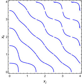
Figure 1: Solutions of the transcendental equation (27) until $x_{j}\sim x_{k}\sim 3$ for $\delta_{A}=1$, for the thin-brane model.

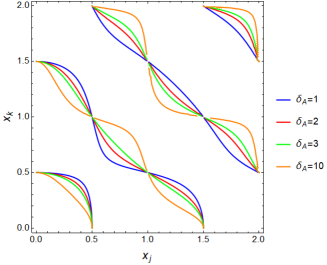
Figure 2: Solutions of the transcendental equation (27) for different values of $\delta_{A}$, for the thin-brane model.

3.2 BLKT at (0,0) and ($\pi R$, $\pi R$)

We consider now branes localized at $(0,0)$ and $(\pi R,\pi R)$ with BLKT on them. For the sake of completeness we add the following term in the Lagrangian

$$\mathcal{L}_{BLKT}= -\frac{1}{4}V_{\mu\nu}V^{\mu\nu}\cdot\Big{[}\delta_{A}R^{2}\,\delta(x^{4},x^{5})$$ (28)

$$+\delta_{B}R^{2}\,\delta(x^{4}-\pi R,x^{5}-\pi R)\Big{]}\,,$$

where $\delta_{A}$ is not necessarily equal to $\delta_{B}$. The equation of motion (19) is modified by an extra term proportional to $\delta_{B}$. The normalization factor has now the following terms

$$Z_{(j,k)}=1+\delta_{A}R^{2}v_{0}^{(j,k)}(0,0)+\delta_{B}R^{2}v_{0}^{(j,k)}(\pi R,\pi R)\,.$$ (29)

The wave-function is equal to Eq. (25) for $x^{4},x^{5}\leq\pi R$, and the transcendental equation is found through the non-continuity of the derivative of the wave-function, whose expression is similar to (3.1). The quantized masses are therefore found through the transcendental equation

$$\left(1+\frac{\delta_{A}\delta_{B}}{4}x_{j}^{2}x_{k}^{2}\right)\cot(x_{j}\pi)\cot(x_{k}\pi)=\frac{x_{j}x_{k}}{2}(\delta_{A}+\delta_{B})\,,$$ (30)

which is reduced to Eq. (27) when $\delta_{B}=0$. This root equation is also similar to the one in the 5-D case Carena:2002me . The solutions of Eq. (30) are depicted in Fig. 3. For lower (higher) values of $\delta_{B}$ the larger (smaller) roots start having the same value, roughly independent of $\delta_{A}$. The case $\delta_{A}=\delta_{B}$ preserves KK-parity and the roots are presented in Fig. 4. Their values are similar to the case $\delta_{B}=0$.

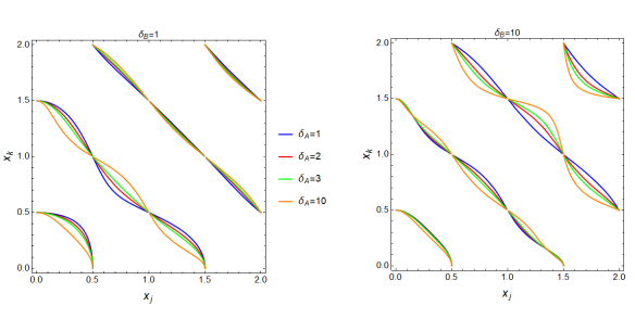
Figure 3: Solutions of the transcendental equation (30) for different values of $\delta_{A}$ and two values of $\delta_{B}$, for the thin-brane model.

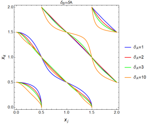
Figure 4: Solutions of the transcendental equation (30) for different values of $\delta_{A}$, when $\delta_{A}=\delta_{B}$, for the thin-brane model.

3.3 BLKT at $(0,\pi R)$

Since the points $(0,\pi R)$ and $(\pi R,0)$ are identified it is sufficient to consider only one case. We will consider now the BLKT inside a brane localized at $(0,\pi R)$, whose Lagrangian is

$$\mathcal{L}_{BLKT}=-\frac{1}{4}V_{\mu\nu}V^{\mu\nu}\cdot\delta_{A}R^{2}\,\delta(x^{4},x^{5}-\pi R)\,.$$ (31)

Similar to the previous cases, the normalization constant becomes

$$Z_{(j,k)}=1+\delta_{A}R^{2}v_{0}^{(j,k)}(0,\pi R)\,.$$ (32)

The solution for the equation of motion with a delta function source at $(0,\pi R)$, satisfying similar BC as Eq. (3.1), is

$$v_{0}^{(j,k)}(x^{4},x^{5})=N_{j,k}\Big{[} \cos(m_{j}x^{4}+m_{k}x^{5})+\cos(m_{k}x^{4}-m_{j}x^{5})$$ (33)

$$+\sin(m_{j}x^{4}+m_{k}x^{5})$$

$$+\sin(m_{k}x^{4}-m_{j}x^{5})\Big{]}\,,$$

where

$$N_{j,k}^{-2} =2\pi^{2}R^{2}\biggr{\{}1+\frac{1}{\pi^{2}(x_{j}^{2}-x_{k}^{2})}+\frac{\sin^{2}(\pi x_{j})\sin(2\pi x_{k})}{2\pi^{2}x_{j}x_{k}}$$ (34)

$$+\frac{\cos(2\pi x_{k})-\sin(2\pi x_{j})}{\pi^{2}(x_{j}^{2}-x_{k}^{2})}$$

$$+\frac{2\cos(\pi x_{k})}{\pi^{2}(x_{j}^{2}-x_{k}^{2})}\Big{[}\sin(\pi x_{j})-\cos(\pi x_{j})\Big{]}\biggr{\}}\,.$$

The dependence of $\delta_{A}$ appears in the transcendental equation, which is identical to Eq. (27), thus having the same solutions for the pair of roots $(x_{j},x_{k})$.

4 BLKT on a thick brane

We consider now the effect of a BLKT on the thick brane, lying between $\pi r<x^{4},x^{5}\leq\pi R$, with a width $\pi(R-r)\equiv\pi L$. The thin brane is obtained in the limit $L\rightarrow 0$. In 5-D, the difference between thin and thick branes leads to the suppressed coupling mechanism Landim:2019epv , existing for branes with a finite thickness. In 6-D, thin branes carry localized operators on the conical singularities at the corners of the square. On the other hand, BLKT are spread inside the thick branes, thus for thin branes the surface terms (2) are non-zero, while for a fat brane the operators are not localized at the conical singularities and there are two regions in the two-dimensional (ED) space, each one having (in principle) vanishing surface terms.

The BLKT with gauge fixing term is Dvali:2000rx ; Dvali:2001ae

$$\mathcal{L}_{TB}=\left[-\frac{1}{4}V_{\mu\nu}V^{\mu\nu}-\frac{1}{2\xi}(\partial_{\mu}V^{\mu})^{2}\right]\cdot\delta_{A}R^{2}\,\theta(x^{4},x^{5})\,,$$ (35)

where the step function is non-zero only inside the thick brane, i.e.

$$\theta(x^{4},x^{5})=\alpha^{2}\quad\text{for }\pi r<x^{4},x^{5}\leq\pi R\,,\qquad$$

$$\theta(x^{4},x^{5})=0\quad\text{for }x^{4},x^{5}<\pi r\,.$$ (36)

The equation of motion for the wave-function inside the thick brane is now

$$\Big{[}\partial_{4}^{2}+\partial_{5}^{2}+(M_{0}^{(j,k)})^{2}+(M_{0}^{(j,k)})^{2}\delta_{A}\alpha^{2}R^{2}\Big{]}\overline{v}_{0}^{(j,k)}(x^{4},x^{5})=0\,.$$ (37)

Similar to the 5-D case Landim:2019epv , we may define an effective mass as $\overline{M}_{0}^{(j,k)}\equiv M_{0}^{(j,k)}\sqrt{1+\delta_{A}\alpha^{2}R^{2}}$, thus the presence of the step-function changes the mass term in the equation of motion for $V_{\mu}^{(j,k)}$ inside the thick brane. It has the same structure of Eq. (12), but with the replacement $M_{0}^{(j,k)}\rightarrow\overline{M}_{0}^{(j,k)}$ Landim:2019epv . Defining the effective mass parameters as

$$\overline{m}_{j}\equiv m_{j}\sqrt{1+\delta_{A}\alpha^{2}R^{2}}\,,\quad\overline{m}_{k}\equiv m_{k}\sqrt{1+\delta_{A}\alpha^{2}R^{2}}\,,$$ (38)

the wave-function inside the thick brane $\overline{v}_{0}^{(j,k)}(x^{4},x^{5})$ has also the same structure of Eq. (14). The wave-function outside the thick brane is

$$v_{0}^{(j,k)}(x^{4},x^{5})=A_{1}^{(j,k)}\left[\cos(m_{j}x^{4}+m_{k}x^{5})\pm\cos(m_{k}x^{4}-m_{j}x^{5})\right]\,,$$ (39)

while inside the thick brane the wave-function is

$$\overline{v}_{0}^{(j,k)}(x^{4},x^{5})=A_{2}^{(j,k)}\left[\cos(\overline{m}_{j}x^{4}+\overline{m}_{k}x^{5})\pm\cos(\overline{m}_{k}x^{4}-\overline{m}_{j}x^{5})\right]\,,$$ (40)

where $A_{1}^{(j,k)}$ and $A_{2}^{(j,k)}$ are coefficients to be determined.

Both wave-functions have this form in order to satisfy the BC (2). The mass parameters, however, should be either $\overline{m}_{i}=m_{i}=i/R$ ($+$) or $\overline{m}_{i}=m_{i}=(i+1/2)/R$ ($-$), for $i=j,k$, in order to satisfy the same BC. This is only possible if $\delta_{A}\alpha=0$. Even if we assume that the fields no longer need to satisfy all previous BC, the situation remains the same by the following reason. The wave-function should be continuous at $(y,\pi r)$ and $(\pi r,y)$, as well as its derivative with respect to both ED coordinates $x^{4}$ and $x^{5}$. Thus $\overline{v}_{0}^{(j,k)}(\pi r,y)=v_{0}^{(j,k)}(\pi r,y)$ and $\partial_{4}\overline{v}_{0}^{(j,k)}|_{(x^{4},x^{5})=(\pi r,y)}=\partial_{4}v_{0}^{(j,k)}|_{(x^{4},x^{5})=(\pi r,y)}$ (the continuity conditions at $(y,\pi r)$ give exactly the same expressions). These conditions can be satisfied at a point $y_{c}$ on the boundary, but it is not possible to match the functions all along the boundary, being the only possibility $\overline{m}_{i}=m_{i}$. Therefore the only viable solution is $\delta_{A}\alpha=0$, which leads to a thin brane.

5 Conclusions

In this paper we have investigated the implications of BLKT on thin and thick branes, for a model of two ED compactified on the chiral square, when a vector field is present in the bulk. For thin branes the presence of BLKT gives mass to all modes of the KK tower of states, being the masses dependent upon the compactification radius and the BLKT parameter. The roots are roughly the same for branes at different positions, i.e., they have similar values for branes localized at $(0,0)$, $(0,\pi R)\sim(\pi R,0)$ and $(\pi R,\pi R)$. The transcendental equations and other relations resemble the 5-D case. The model presents the usual behavior of quantum systems in two dimensions, i.e., there are $(2n+1)$ quantized masses for each curve $n$, and each mode is described by the segments in the dashed lines: one massive zero-mode $M_{0,0}$ at $n=0$, three quantized masses $M_{0,1}$, $M_{1,0}$ and $M_{1,1}$ at $n=1$ (being $M_{0,1}$ and $M_{1,0}$ degenerate), etc.

The BLKT on thick branes, on the other hand, does not provide a non-trivial result $\delta_{A}\alpha\neq 0$ due to the BC. This scenario is similar to the refraction of a wave-function by a two-dimensional step function. Suppose an incident wave-function $e^{i(k_{x}x+k_{y}y)}$, a refracted wave $e^{i(q_{x}x+q_{y}y)}$ and a step-function different from zero for $x>0$. The BC implies that $k_{y}=q_{y}$ and the analogue situation in our problem is therefore $\bar{m}_{i}=m_{i}$. Hence the mechanism of suppressed coupling in 5-D Landim:2019epv cannot be applied in 6-D.

The results presented here works for different fields in the bulk and can be used in several further proposals, as for instance, in a model of ED with the dark photon as mediator. This model was done in 5-D Rizzo:2018joy ; Rizzo:2018ntg , but an extension might be able with two ED as well, or even its inclusion in the UED model. In both cases, the BLKT breaks the extra $U(1)_{D}$ gauge symmetry via BC without adding an extra Higgs-like field, avoiding, in turn, constraints on the Higgs-portal coupling. Potential signatures for such massive spin-1 KK particles depend upon the specific model considered but it usually includes missing energy searches, which might constrain the two parameters in this model.

- [1] Ricardo G. Landim and Thomas G. Rizzo. Thick Branes in Extra Dimensions and Suppressed Dark Couplings. JHEP, 06:112, 2019.
- [2] Ignatios Antoniadis. A Possible new dimension at a few TeV. Phys. Lett., B246:377–384, 1990.
- [3] Keith R. Dienes, Emilian Dudas, and Tony Gherghetta. Extra space-time dimensions and unification. Phys. Lett., B436:55–65, 1998.
- [4] Ignatios Antoniadis, Nima Arkani-Hamed, Savas Dimopoulos, and G. R. Dvali. New dimensions at a millimeter to a Fermi and superstrings at a TeV. Phys. Lett., B436:257–263, 1998.
- [5] Nima Arkani-Hamed, Savas Dimopoulos, and G. R. Dvali. The Hierarchy problem and new dimensions at a millimeter. Phys. Lett., B429:263–272, 1998.
- [6] Lisa Randall and Raman Sundrum. A Large mass hierarchy from a small extra dimension. Phys. Rev. Lett., 83:3370–3373, 1999.
- [7] Nima Arkani-Hamed, Timothy Cohen, Raffaele Tito D’Agnolo, Anson Hook, Hyung Do Kim, and David Pinner. Solving the Hierarchy Problem at Reheating with a Large Number of Degrees of Freedom. Phys. Rev. Lett., 117(25):251801, 2016.
- [8] Kaustubh Agashe, Gilad Perez, and Amarjit Soni. Flavor structure of warped extra dimension models. Phys. Rev., D71:016002, 2005.
- [9] Stephan J. Huber. Flavor violation and warped geometry. Nucl. Phys., B666:269–288, 2003.
- [10] A. Liam Fitzpatrick, Gilad Perez, and Lisa Randall. Flavor anarchy in a Randall-Sundrum model with 5D minimal flavor violation and a low Kaluza-Klein scale. Phys. Rev. Lett., 100:171604, 2008.
- [11] Thomas Appelquist, Bogdan A. Dobrescu, Eduardo Ponton, and Ho-Ung Yee. Proton stability in six-dimensions. Phys. Rev. Lett., 87:181802, 2001.
- [12] Nima Arkani-Hamed, Hsin-Chia Cheng, Bogdan A. Dobrescu, and Lawrence J. Hall. Selfbreaking of the standard model gauge symmetry. Phys. Rev., D62:096006, 2000.
- [13] Michio Hashimoto, Masaharu Tanabashi, and Koichi Yamawaki. Top mode standard model with extra dimensions. Phys. Rev., D64:056003, 2001.
- [14] Csaba Csaki, Christophe Grojean, and Hitoshi Murayama. Standard model Higgs from higher dimensional gauge fields. Phys. Rev., D67:085012, 2003.
- [15] C. A. Scrucca, M. Serone, L. Silvestrini, and A. Wulzer. Gauge Higgs unification in orbifold models. JHEP, 02:049, 2004.
- [16] Arthur Hebecker and John March-Russell. The structure of GUT breaking by orbifolding. Nucl. Phys., B625:128–150, 2002.
- [17] Lawrence J. Hall, Yasunori Nomura, Takemichi Okui, and David Tucker-Smith. SO(10) unified theories in six-dimensions. Phys. Rev., D65:035008, 2002.
- [18] T. Asaka, W. Buchmuller, and L. Covi. Bulk and brane anomalies in six-dimensions. Nucl. Phys., B648:231–253, 2003.
- [19] T. Asaka, W. Buchmuller, and L. Covi. Quarks and leptons between branes and bulk. Phys. Lett., B563:209–216, 2003.
- [20] Bogdan A. Dobrescu and Erich Poppitz. Number of fermion generations derived from anomaly cancellation. Phys. Rev. Lett., 87:031801, 2001.
- [21] M. Fabbrichesi, M. Piai, and G. Tasinato. Axion and neutrino physics from anomaly cancellation. Phys. Rev., D64:116006, 2001.
- [22] Nicolas Borghini, Yves Gouverneur, and Michel H. G. Tytgat. Anomalies and fermion content of grand unified theories in extra dimensions. Phys. Rev., D65:025017, 2002.
- [23] M. Fabbrichesi, R. Percacci, M. Piai, and M. Serone. Cancellation of global anomalies in spontaneously broken gauge theories. Phys. Rev., D66:105028, 2002.
- [24] J. M. Frere, M. V. Libanov, and Sergey V. Troitsky. Neutrino masses with a single generation in the bulk. JHEP, 11:025, 2001.
- [25] T. Watari and T. Yanagida. Higher dimensional supersymmetry as an origin of the three families for quarks and leptons. Phys. Lett., B532:252–258, 2002.
- [26] Thomas Appelquist, Hsin-Chia Cheng, and Bogdan A. Dobrescu. Bounds on universal extra dimensions. Phys. Rev., D64:035002, 2001.
- [27] Bogdan A. Dobrescu and Eduardo Ponton. Chiral compactification on a square. JHEP, 03:071, 2004.
- [28] Gustavo Burdman, Bogdan A. Dobrescu, and Eduardo Ponton. Six-dimensional gauge theory on the chiral square. JHEP, 02:033, 2006.
- [29] Eduardo Ponton and Lin Wang. Radiative effects on the chiral square. JHEP, 11:018, 2006.
- [30] Gustavo Burdman, Bogdan A. Dobrescu, and Eduardo Ponton. Resonances from two universal extra dimensions. Phys. Rev., D74:075008, 2006.
- [31] Georges Aad et al. Search for squarks and gluinos in events with isolated leptons, jets and missing transverse momentum at TeV with the ATLAS detector. JHEP, 04:116, 2015.
- [32] The ATLAS collaboration. Search for squarks and gluinos in events with isolated leptons, jets and missing transverse momentum at TeV with the ATLAS detector. 2013.
- [33] Nicolas Deutschmann, Thomas Flacke, and Jong Soo Kim. Current LHC Constraints on Minimal Universal Extra Dimensions. Phys. Lett., B771:515–520, 2017.
- [34] Jyotiranjan Beuria, AseshKrishna Datta, Dipsikha Debnath, and Konstantin T. Matchev. LHC Collider Phenomenology of Minimal Universal Extra Dimensions. Comput. Phys. Commun., 226:187–205, 2018.
- [35] M. Tanabashi et al. Review of Particle Physics. Phys. Rev., D98(3):030001, 2018.
- [36] G. Burdman, O. J. P. Eboli, and D. Spehler. Signals of Two Universal Extra Dimensions at the LHC. Phys. Rev., D94(9):095004, 2016.
- [37] G. R. Dvali, Gregory Gabadadze, and Massimo Porrati. 4-D gravity on a brane in 5-D Minkowski space. Phys. Lett., B485:208–214, 2000.
- [38] G. R. Dvali, Gregory Gabadadze, and Mikhail A. Shifman. (Quasi)localized gauge field on a brane: Dissipating cosmic radiation to extra dimensions? Phys. Lett., B497:271–280, 2001.
- [39] G. R. Dvali and Gregory Gabadadze. Gravity on a brane in infinite volume extra space. Phys. Rev., D63:065007, 2001.
- [40] Gia Dvali, Gregory Gabadadze, Xin-rui Hou, and Emiliano Sefusatti. Seesaw modification of gravity. Phys. Rev., D67:044019, 2003.
- [41] Gia Dvali, Gregory Gabadadze, and M. Shifman. Diluting cosmological constant in infinite volume extra dimensions. Phys. Rev., D67:044020, 2003.
- [42] Marcela Carena, Timothy M. P. Tait, and C. E. M. Wagner. Branes and orbifolds are opaque. Acta Phys. Polon., B33:2355, 2002.
- [43] Marcela Carena, Eduardo Ponton, Timothy M. P. Tait, and C. E. M Wagner. Opaque Branes in Warped Backgrounds. Phys. Rev., D67:096006, 2003.
- [44] F. del Aguila, M. Perez-Victoria, and Jose Santiago. Physics of brane kinetic terms. Acta Phys. Polon., B34:5511–5522, 2003.
- [45] F. del Aguila, M. Perez-Victoria, and Jose Santiago. Bulk fields with general brane kinetic terms. JHEP, 02:051, 2003.
- [46] H. Davoudiasl, J. L. Hewett, and T. G. Rizzo. Brane localized kinetic terms in the Randall-Sundrum model. Phys. Rev., D68:045002, 2003.
- [47] H. Davoudiasl, J. L. Hewett, and T. G. Rizzo. Brane localized curvature for warped gravitons. JHEP, 08:034, 2003.
- [48] Thomas G. Rizzo. Kinetic mixing, dark photons and an extra dimension. Part I. JHEP, 07:118, 2018.
- [49] Thomas G. Rizzo. Kinetic mixing, dark photons and extra dimensions. Part II: fermionic dark matter. JHEP, 10:069, 2018.
- [50] G. R. Dvali and S. H. Henry Tye. Brane inflation. Phys. Lett., B450:72–82, 1999.
- [51] G. Alencar, R. R. Landim, M. O. Tahim, and R. N. Costa Filho. Gauge Field Localization on the Brane Through Geometrical Coupling. Phys. Lett., B739:125–127, 2014.
- [52] G. Alencar. Hidden conformal symmetry in Randall–Sundrum 2 model: Universal fermion localization by torsion. Phys. Lett., B773:601–603, 2017.
- [53] G. Alencar, R. R. Landim, C. R. Muniz, and R. N. Costa Filho. Nonminimal couplings in Randall-Sundrum scenarios. Phys. Rev., D92(6):066006, 2015.
- [54] G. Alencar, C. R. Muniz, R. R. Landim, I. C. Jardim, and R. N. Costa Filho. Photon mass as a probe to extra dimensions. Phys. Lett., B759:138–140, 2016.
- [55] G. Alencar, I. C. Jardim, R. R. Landim, C. R. Muniz, and R. N. Costa Filho. Generalized nonminimal couplings in Randall-Sundrum scenarios. Phys. Rev., D93(12):124064, 2016.
- [56] G. Alencar, I. C. Jardim, and R. R. Landim. -Forms non-minimally coupled to gravity in Randall–Sundrum scenarios. Eur. Phys. J., C78(5):367, 2018.
- [57] Luiz F. Freitas, G. Alencar, and R. R. Landim. Universal Aspects of Gauge Field Localization on Branes in -dimensions. JHEP, 02:035, 2019.
- [58] A. De Rujula, A. Donini, M. B. Gavela, and S. Rigolin. Fat brane phenomena. Phys. Lett., B482:195–204, 2000.
- [59] Howard Georgi, Aaron K. Grant, and Girma Hailu. Chiral fermions, orbifolds, scalars and fat branes. Phys. Rev., D63:064027, 2001.
- [60] V. Silveira and A. Zee. Scalar Phantoms. Phys. Lett., 161B:136–140, 1985.
- [61] J. McDonald. Gauge singlet scalars as cold dark matter. Phys. Rev., D50:3637–3649, 1994.
- [62] C. P. Burgess, M. Pospelov, and T. ter Veldhuis. The Minimal model of nonbaryonic dark matter: A Singlet scalar. Nucl. Phys., B619:709–728, 2001.
- [63] M. C. Bento, O. Bertolami, R. Rosenfeld, and L. Teodoro. Selfinteracting dark matter and invisibly decaying Higgs. Phys. Rev., D62:041302, 2000.
- [64] O. Bertolami and R. Rosenfeld. The Higgs portal and an unified model for dark energy and dark matter. Int. J. Mod. Phys., A23:4817–4827, 2008.
- [65] M. C. Bento, O. Bertolami, and R. Rosenfeld. Cosmological constraints on an invisibly decaying Higgs boson. Phys. Lett., B518:276–281, 2001.
- [66] J. March-Russell, S. M. West, D. Cumberbatch, and D. Hooper. Heavy Dark Matter Through the Higgs Portal. JHEP, 07:058, 2008.
- [67] A. Biswas and D. Majumdar. The Real Gauge Singlet Scalar Extension of Standard Model: A Possible Candidate of Cold Dark Matter. Pramana, 80:539–557, 2013.
- [68] R. Costa, A. P. Morais, M. O. P. Sampaio, and R. Santos. Two-loop stability of a complex singlet extended Standard Model. Phys. Rev., D92:025024, 2015.
- [69] A. Eichhorn and M. M. Scherer. Planck scale, Higgs mass, and scalar dark matter. Phys. Rev., D90(2):025023, 2014.
- [70] N. Khan and S. Rakshit. Study of electroweak vacuum metastability with a singlet scalar dark matter. Phys. Rev., D90(11):113008, 2014.
- [71] F. S. Queiroz and K. Sinha. The Poker Face of the Majoron Dark Matter Model: LUX to keV Line. Phys. Lett., B735:69–74, 2014.
- [72] C. Kouvaris, I. M. Shoemaker, and K. Tuominen. Self-Interacting Dark Matter through the Higgs Portal. Phys. Rev., D91(4):043519, 2015.
- [73] S. Bhattacharya, S. Jana, and S. Nandi. Neutrino Masses and Scalar Singlet Dark Matter. Phys. Rev., D95(5):055003, 2017.
- [74] O. Bertolami, C. Cosme, and J. G. Rosa. Scalar field dark matter and the Higgs field. Phys. Lett., B759:1–8, 2016.
- [75] R. Campbell, S. Godfrey, H. E. Logan, and A. Poulin. Real singlet scalar dark matter extension of the Georgi-Machacek model. Phys. Rev., D95(1):016005, 2017.
- [76] M. Heikinheimo, T. Tenkanen, K. Tuominen, and V Vaskonen. Observational Constraints on Decoupled Hidden Sectors. Phys. Rev., D94(6):063506, 2016. [Erratum: Phys. Rev.D96,no.10,109902(2017)].
- [77] K. Kainulainen, S. Nurmi, T. Tenkanen, K. Tuominen, and V. Vaskonen. Isocurvature Constraints on Portal Couplings. JCAP, 1606(06):022, 2016.
- [78] S. Nurmi, T. Tenkanen, and K. Tuominen. Inflationary Imprints on Dark Matter. JCAP, 1511(11):001, 2015.
- [79] T. Tenkanen. Feebly Interacting Dark Matter Particle as the Inflaton. JHEP, 09:049, 2016.
- [80] J. A. Casas, D. G. Cerdeño, J. M. Moreno, and J. Quilis. Reopening the Higgs portal for single scalar dark matter. JHEP, 05:036, 2017.
- [81] Catarina Cosme, João G. Rosa, and O. Bertolami. Scalar field dark matter with spontaneous symmetry breaking and the keV line. Phys. Lett., B781:639–644, 2018.
- [82] M. Heikinheimo, T. Tenkanen, and K. Tuominen. WIMP miracle of the second kind. Phys. Rev., D96(2):023001, 2017.
- [83] Ricardo G. Landim. Dark energy, scalar singlet dark matter and the Higgs portal. Mod. Phys. Lett., A33(15):1850087, 2018.
- [84] Bob Holdom. Two U(1)’s and Epsilon Charge Shifts. Phys. Lett., 166B:196–198, 1986.
- [85] Bob Holdom. Searching for Charges and a New U(1). Phys. Lett., B178:65–70, 1986.
- [86] Keith R. Dienes, Christopher F. Kolda, and John March-Russell. Kinetic mixing and the supersymmetric gauge hierarchy. Nucl. Phys., B492:104–118, 1997.
- [87] F. Del Aguila. The Physics of z-prime bosons. Acta Phys. Polon., B25:1317–1336, 1994.
- [88] K. S. Babu, Christopher F. Kolda, and John March-Russell. Leptophobic U(1) and the R() - R() crisis. Phys. Rev., D54:4635–4647, 1996.
- [89] Thomas G. Rizzo. Gauge kinetic mixing and leptophobic in E(6) and SO(10). Phys. Rev., D59:015020, 1998.
- [90] Daniel Feldman, Boris Kors, and Pran Nath. Extra-weakly Interacting Dark Matter. Phys. Rev., D75:023503, 2007.
- [91] Daniel Feldman, Zuowei Liu, and Pran Nath. The Stueckelberg Z-prime Extension with Kinetic Mixing and Milli-Charged Dark Matter From the Hidden Sector. Phys. Rev., D75:115001, 2007.
- [92] Maxim Pospelov, Adam Ritz, and Mikhail B. Voloshin. Secluded WIMP Dark Matter. Phys. Lett., B662:53–61, 2008.
- [93] Maxim Pospelov. Secluded U(1) below the weak scale. Phys. Rev., D80:095002, 2009.
- [94] Hooman Davoudiasl, Hye-Sung Lee, and William J. Marciano. Muon Anomaly and Dark Parity Violation. Phys. Rev. Lett., 109:031802, 2012.
- [95] Hooman Davoudiasl, Hye-Sung Lee, and William J. Marciano. ’Dark’ Z implications for Parity Violation, Rare Meson Decays, and Higgs Physics. Phys. Rev., D85:115019, 2012.
- [96] Rouven Essig et al. Working Group Report: New Light Weakly Coupled Particles. In Proceedings, 2013 Community Summer Study on the Future of U.S. Particle Physics: Snowmass on the Mississippi (CSS2013): Minneapolis, MN, USA, July 29-August 6, 2013, 2013.
- [97] Eder Izaguirre, Gordan Krnjaic, Philip Schuster, and Natalia Toro. Analyzing the Discovery Potential for Light Dark Matter. Phys. Rev. Lett., 115(25):251301, 2015.
- [98] Michael Duerr, Pavel Fileviez Pérez, and Juri Smirnov. Scalar Dark Matter: Direct vs. Indirect Detection. JHEP, 06:152, 2016.
- [99] P. Athron et al. Status of the scalar singlet dark matter model. Eur. Phys. J., C77(8):568, 2017.
- [100] A. Djouadi, O. Lebedev, Y. Mambrini, and J. Quevillon. Implications of LHC searches for Higgs–portal dark matter. Phys. Lett., B709:65–69, 2012.
- [101] K. Cheung, Y.-L. S. Tsai, P.-Y. Tseng, T.-C. Yuan, and A. Zee. Global Study of the Simplest Scalar Phantom Dark Matter Model. JCAP, 1210:042, 2012.
- [102] A. Djouadi, A. Falkowski, Y. Mambrini, and J. Quevillon. Direct Detection of Higgs-Portal Dark Matter at the LHC. Eur. Phys. J., C73(6):2455, 2013.
- [103] J. M. Cline, K. Kainulainen, P. Scott, and C. Weniger. Update on scalar singlet dark matter. Phys. Rev., D88:055025, 2013. [Erratum: Phys. Rev.D92,no.3,039906(2015)].
- [104] M. Endo and Y. Takaesu. Heavy WIMP through Higgs portal at the LHC. Phys. Lett., B743:228–234, 2015.
- [105] A. Goudelis, Y. Mambrini, and C. Yaguna. Antimatter signals of singlet scalar dark matter. JCAP, 0912:008, 2009.
- [106] A. Urbano and W. Xue. Constraining the Higgs portal with antiprotons. JHEP, 03:133, 2015.
- [107] D. S. Akerib et al. Improved Limits on Scattering of Weakly Interacting Massive Particles from Reanalysis of 2013 LUX Data. Phys. Rev. Lett., 116(16):161301, 2016.
- [108] X.-G. He and J. Tandean. New LUX and PandaX-II Results Illuminating the Simplest Higgs-Portal Dark Matter Models. JHEP, 12:074, 2016.
- [109] M. Escudero, A. Berlin, D. Hooper, and M.-X. Lin. Toward (Finally!) Ruling Out Z and Higgs Mediated Dark Matter Models. JCAP, 1612:029, 2016.
- [110] P. A. R. Ade et al. Planck 2015 results. XIII. Cosmological parameters. Astron. Astrophys., 594:A13, 2016.
- [111] J. M. Cline and P. Scott. Dark Matter CMB Constraints and Likelihoods for Poor Particle Physicists. JCAP, 1303:044, 2013. [Erratum: JCAP1305,E01(2013)].
- [112] T. R. Slatyer. Indirect dark matter signatures in the cosmic dark ages. I. Generalizing the bound on s-wave dark matter annihilation from Planck results. Phys. Rev., D93(2):023527, 2016.
- [113] M. Ackermann et al. Searching for Dark Matter Annihilation from Milky Way Dwarf Spheroidal Galaxies with Six Years of Fermi Large Area Telescope Data. Phys. Rev. Lett., 115(23):231301, 2015.
- [114] D. S. Akerib et al. Results from a search for dark matter in the complete LUX exposure. Phys. Rev. Lett., 118(2):021303, 2017.
- [115] A. Tan et al. Dark Matter Results from First 98.7 Days of Data from the PandaX-II Experiment. Phys. Rev. Lett., 117(12):121303, 2016.
- [116] R. Agnese et al. Search for Low-Mass Weakly Interacting Massive Particles with SuperCDMS. Phys. Rev. Lett., 112(24):241302, 2014.
- [117] E. Aprile et al. Dark Matter Results from 225 Live Days of XENON100 Data. Phys. Rev. Lett., 109:181301, 2012.
- [118] M. G. Aartsen et al. Search for dark matter annihilations in the Sun with the 79-string IceCube detector. Phys. Rev. Lett., 110(13):131302, 2013.
- [119] M. G. Aartsen et al. Improved limits on dark matter annihilation in the Sun with the 79-string IceCube detector and implications for supersymmetry. JCAP, 1604(04):022, 2016.
- [120] Marco Battaglieri et al. US Cosmic Visions: New Ideas in Dark Matter 2017: Community Report. In U.S. Cosmic Visions: New Ideas in Dark Matter College Park, MD, USA, March 23-25, 2017, 2017.
- [121] E. M. Riordan et al. A Search for Short Lived Axions in an Electron Beam Dump Experiment. Phys. Rev. Lett., 59:755, 1987.
- [122] J. D. Bjorken, S. Ecklund, W. R. Nelson, A. Abashian, C. Church, B. Lu, L. W. Mo, T. A. Nunamaker, and P. Rassmann. Search for Neutral Metastable Penetrating Particles Produced in the SLAC Beam Dump. Phys. Rev., D38:3375, 1988.
- [123] A. Bross, M. Crisler, Stephen H. Pordes, J. Volk, S. Errede, and J. Wrbanek. A Search for Shortlived Particles Produced in an Electron Beam Dump. Phys. Rev. Lett., 67:2942–2945, 1991.
- [124] James D. Bjorken, Rouven Essig, Philip Schuster, and Natalia Toro. New Fixed-Target Experiments to Search for Dark Gauge Forces. Phys. Rev., D80:075018, 2009.
- [125] Hooman Davoudiasl, Hye-Sung Lee, and William J. Marciano. Dark Side of Higgs Diphoton Decays and Muon g-2. Phys. Rev., D86:095009, 2012.
- [126] Motoi Endo, Koichi Hamaguchi, and Go Mishima. Constraints on Hidden Photon Models from Electron g-2 and Hydrogen Spectroscopy. Phys. Rev., D86:095029, 2012.
- [127] D. Babusci et al. Limit on the production of a light vector gauge boson in phi meson decays with the KLOE detector. Phys. Lett., B720:111–115, 2013.
- [128] F. Archilli et al. Search for a vector gauge boson in meson decays with the KLOE detector. Phys. Lett., B706:251–255, 2012.
- [129] P. Adlarson et al. Search for a dark photon in the decay. Phys. Lett., B726:187–193, 2013.
- [130] S. Abrahamyan et al. Search for a New Gauge Boson in Electron-Nucleus Fixed-Target Scattering by the APEX Experiment. Phys. Rev. Lett., 107:191804, 2011.
- [131] H. Merkel et al. Search for Light Gauge Bosons of the Dark Sector at the Mainz Microtron. Phys. Rev. Lett., 106:251802, 2011.
- [132] Matthew Reece and Lian-Tao Wang. Searching for the light dark gauge boson in GeV-scale experiments. JHEP, 07:051, 2009.
- [133] Bernard Aubert et al. Search for Dimuon Decays of a Light Scalar Boson in Radiative Transitions Upsilon —> gamma A0. Phys. Rev. Lett., 103:081803, 2009.
- [134] Herbert K. Dreiner, Jean-François Fortin, Christoph Hanhart, and Lorenzo Ubaldi. Supernova constraints on MeV dark sectors from annihilations. Phys. Rev., D89(10):105015, 2014.