Constrained Clustering: General Pairwise and Cardinality Constraints

Abstract

In this work, we study constrained clustering, where constraints are utilized to guide the clustering process. In existing works, two categories of constraints have been widely explored, namely pairwise and cardinality constraints. Pairwise constraints enforce the cluster labels of two instances to be the same (must-link constraints) or different (cannot-link constraints). Cardinality constraints encourage cluster sizes to satisfy a user-specified distribution. However, most existing constrained clustering models can only utilize one category of constraints at a time. In this paper, we enforce the above two categories into a unified clustering model starting with the integer program formulation of the standard K-means. As these two categories provide useful information at different levels, utilizing both of them is expected to allow for better clustering performance. However, the optimization is difficult due to the binary and quadratic constraints in the proposed unified formulation. To alleviate this difficulty, we utilize two techniques: equivalently replacing the binary constraints by the intersection of two continuous constraints; the other is transforming the quadratic constraints into bi-linear constraints by introducing extra variables. Then we derive an equivalent continuous reformulation with simple constraints, which can be efficiently solved by Alternating Direction Method of Multipliers (ADMM) algorithm. Extensive experiments on both synthetic and real data demonstrate: (1) when utilizing a single category of constraint, the proposed model is superior to or competitive with state-of-the-art constrained clustering models, and (2) when utilizing both categories of constraints jointly, the proposed model shows better performance than the case of the single category. The experimental results show that the proposed method exploits the constraints to achieve perfect clustering performance with improved clustering to $2-5$% in classical clustering metrics, e.g. Adjusted Random Index (ARI), Mirkin’s Index (MI), and Huber’s Index (HI), outerperfomring all compared-againts methods across the board. Moreover, we show that our method is robust to initialization.

=-15pt

I Introduction

Clustering is the task of partitioning data into different clusters, based on some specific cluster assumptions. For example, K-means and Gaussian mixture models (GMM) assume each cluster is sampled from a Gaussian distribution. In contrast, density-based clustering assumes that the densities of data points in different clusters should be different, such as Chameleon [1] and AITC [2], or clusters should be partitioned at low density regions [3]. However, if the adopted cluster assumption is not suited to the target dataset, this may result in a poor performance. To avoid such performance instability, prior knowledge or constraints on the data can be used to guide the clustering process. These constraints are independent of cluster assumptions, and they provide weak supervision to reflect user preferences. Thus, clustering with constraints, called constrained clustering, [4, 5, 6], is expected to give better and more stable performance than unconstrained clustering.

Two main categories of constraints have been widely studied in the field of constrained clustering, namely pairwise and cardinality constraints. Pairwise constraints may arise from some form of perceived similarity between samples. For instance, the continuity property is a form of Pairwise constraints that suggests that neighbouring samples are likely to be clustered together and vice versa. Thus, Pairwise constraints include must-link and cannot-link constraints. Must-link constraints enforce that a set of pairs of instances should be in the same cluster, while cannot-link constraints enforce that they belong to different clusters. Thereafter, this category can be viewed as instance-level constraints. On the other hand, Cardinality constraints provide extra knowledge on the size distribution of all clusters. This sort of constraints become particularly necessary in clustering tasks of data that is high dimensional and sparse with many clusters to assign [7]. This often leads to solutions of empty clusters or unbalanced cluster assignments. Balancing constraints that lead to equal sized clusters are only a special case of Cardinality constraints. This category in general can be viewed as cluster-level constraints.

Many clustering methods have been proposed to utilize one of the two categories of constraints, such as the ones with pairwise constraints [8, 9, 10, 11, 12, 6, 13, 5, 4], and the ones with cardinality constraints [14, 15, 7, 16]. However, in some cases, one might want to enforce the continuity property among a set of points and the same time requiring to have solutions of balanced or user specified cluster sizes. In general, both constraints can be provided simultaneously, as they are derived from different sources. For example, pairwise constraints are usually obtained from an oracle query, while cardinality constraints can be obtained from experience or user preference. Moreover, they represent supervision at different levels. Each of them can provide particularly useful information that is not covered by the other. Thus, having both sets of constraints together in a clustering task should signifecently improve the performance and to the best of our knowledge, there is no existing work that can seamlessly incorporate both categories jointly.

For existing constrained clustering methods that handle one constraint category, it is non-trivial to directly add the other. For example, embedding cardinality constraints into the COP-KMEANS [13], will lead to instability in performance where COP-KMEANS will often fail in finding a feasible solution. This is because COP-KMEANS is very sensitive to cluster initialization. Moreover, it is also not easy to embed the pairwise constraints into normalized/ratio-cut [16], which exploits balanced distribution constraints. In short, existing models are designed to exploit one category of constraints at a time.

We propose a unified model to incorporate both categories of constraints to guide the clustering process. Specifically, we start from the formulation of the standard K-mean method, and formulate cardinality constraints into linear constraints and pairwise constraints into quadratic constraints. Then we obtain a discrete optimization problem with quadratic constraints, which is difficult to be solved by off-the-shelf optimization methods. Thus we propose to utilize two techniques. One is to equivalently replace the binary constraints by the intersection of two continuous constraints, which was firstly proposed in [17]. The other is to transform the quadratic constraints to bi-linear constraints by introducing extra variables. Our key contributions revolve around the new novel continuious reformulation for the K-Means problem allowing to incorporate both cardinality and pair-wise constraints. The reformulation is simple, flexible, and enjoys nice convergence properties with competitive performance. The contributions can be summarized in three folds.

• We embed both pairwise and cardinality constraints into one unified clustering model. To the best of our knowledge, this is the first attempt in the field of constrained clustering.

• We propose to equivalently transform the binary and quadratic constraints in the original problem to continuous and bi-linear constraints, to obtain a simple continuous reformulation.

• We conduct various experiments on several synthetic and real datasets comparing against 5 different algorithms. Our approach demonstrate competitive edge over all compared-against methods in the final clustering performance while respecting the imposed constraints.

II Related Work

Here, we briefly review existing clustering models that utilize pairwise or cardinality constraints.

Pairwise Constraints. They were first introduced into clustering in [4] and [13]. In [4], a method called COP-COBWEB inserted the pairwise constraints into the clustering process of the incremental clustering method COBWEB [18], which utilizes four operators (i.e. add, new, merge, and split) to maximize the intra-cluster similarity and the inter-cluster dissimilarity. In each operator of COP-COBWEB, the given pairwise constraints are checked to ensure the satisfaction of all constraints. In [13], the method COP-KMEANS checks the pairwise constraints in each assignment step of K-means. Both COP-COBWEB and COP-KMEANS treat the pairwise constraints as hard constraints (i.e. all constraints must be satisfied), and the constraints are somewhat independent of the original objective. A common limitation of these two methods is that the processing order of instances influences clustering performance, and sometimes they may even fail to output a feasible partition.

To avoid this limitation, many methods treat pairwise constraints as soft constraints (i.e. a subset of these constraints could be violated) to develop more flexible approaches to embed constraints. For example, in constrained complete-link (CCL) [5], pairwise constraints are used to modify the instance proximity computed in the original feature space. Then, standard complete-link clustering is applied using the modified proximity matrix. Penalized probabilistic clustering (PPC) [10] uses pairwise constraints as a prior term w.r.t. the cluster labels within the underlying GMM-based model. Clustering configurations not satisfying the constraints have a lower probability. Moreover, HMRF-KMEANS [19] embeds pairwise constraints as correlations between cluster labels in a hidden Markov random field (HMRF). A metric learning step is added into standard K-means to encourage gradual satisfaction of pairwise constraints. Other methods propagate pairwise constraints via instance similarity to obtain soft constraints, such as constrained spectral clustering [8] and HMRF-pc [12, 20].

Cardinality Constraints. They are widely used to guide the clustering process. Balancing constraints are a special type that encourages all clusters to be balanced in size or in connecting weights. For example, normalized cuts [16] divides the standard cut cost (sum of edge weights connecting the two clusters) by the sum of edge weights between each cluster and all other instances. Hence, each cluster is encouraged to have similar edge weights connecting to other clusters. Similarly, ratio cut [21] normalizes the cut function by the size of each cluster to encourage similar sized clusters. Equi-sized Fuzzy c-means (FCM) [15] formulates the balancing constraints as equality constraints, where the size of each cluster equals to the average cluster size. More general cardinality constraints have also been explored. For example, a constrained K-means method [7] sets a lower bound on the cluster size, to avoid very small or empty clusters that occur in standard K-means. An extension of the Equi-sized FCM is proposed in [14], where the size of one single cluster is set to a specific size.

To the best of our knowledge, the only clustering frameworks that enable both sets of constraints (Cardinality and Pairwise) either target a very specific class of methods that suffer from the locality property [22], or are greedy heuristics that propagate constraints [23]. Clustering methods that suffer from the locality property result in clusters located partially or entirely outside the Voronoi cell of their centers [22]. However, popular methods like K-means, K-medians, and many others always satisfy the locality property by definition, thus, limiting the theoretical results of [22] to a smaller class of clustering methods. There has also been an attempt to use standard constraint propagation methods to enforce both classes of constraints [23]. However, this is done in a greedy heuristic fashion that may often fail in finding a feasible solution. Therefore, we believe that the combination of both pairwise and cardinality categories into a constraint generic and unified clustering model that can be systematically solved (ie using a flexible continuous optimization framework) has not been explored in any existing work.

III Proposed Method

Unlike previous methods that can only handle either pairwise or cardinality constraints, we show, in this section, a detailed derivation of our framework that embeds both constraints simultaneously. In fact, this formulation is flexible and generic enough to handle any other linear equality. In our framework, we adopt the K-means integer program formulation [24] expressed as follows:

$$\min_{\{x_{ij}\}_{i=1,j=1}^{n,k}}~{}~{}~{}\sum_{j=1}^{k}\sum_{i=1}^{n}x_{ij}\Big{|}\Big{|}\mathbf{s}_{i}-\frac{\sum_{p=1}^{n}x_{pj}\mathbf{s}_{p}}{\sum_{l=1}^{n}x_{lj}}\Big{|}\Big{|}_{2}^{2}$$ (1)

$$\text{s.t.}\ \sum_{j=1}^{k}x_{ij}=1,\ \ \forall\ \ i\ \ x_{ij}\in\{0,1\}\ \forall\ i,j$$

where $\mathbf{s}_{p}\in\mathbb{R}^{d}$ is the $p^{\text{th}}$ data point to be clustered and $k$ is the number of clusters. The variable $x_{ij}$ defines the binary association between data point $i$ and cluster $j$. The constraint $\sum_{j=1}^{k}x_{ij}=1$ enforces data point $i$ to belong to one and only one cluster. This constraint can be simply written as a matrix vector multiplication: $\Psi^{\top}\mathbf{x}=\mathbf{1}_{n}$, where $\Psi^{\top}\in\mathbb{R}^{n\times nk}$ is a binary matrix that has in each row a vector $\mathbf{1}_{k}^{\top}$ that sums all the binary labels for a given data point while the rest are 0.

To simplify the fractional objective, we introduce variable $w_{pj}$, such that: $x_{pj}=w_{pj}\sum_{l=1}^{n}x_{lj}$. For ease of notation, we concatenate all the binary labels $x_{ij}$ into one vector ordered by the data points one at a time as follows: $\mathbf{x}^{\top}=\begin{bmatrix}(x_{11}&\ldots&x_{1k})&\ldots&(x_{n1}&\ldots&x_{nk})\end{bmatrix}^{\top}$. We also concatenate and reorder the $w_{pj}$ values one cluster at a time: $\mathbf{w}^{\top}=\begin{bmatrix}(w_{11}&\ldots&w_{n1})&\ldots&(w_{1k}&\ldots&w_{nk})\end{bmatrix}^{\top}$. A matrix $\mathbf{P}\in\mathbb{R}^{nk\times nk}$ is used to swap the order of the binary vectors from a cluster based order to a data point order and vice versa. Note that $\mathbf{P}$ is a proper permutation matrix that is symmetric and it satisfies: $\mathbf{P}\mathbf{P}^{\top}=\mathbf{I}_{nk}$. Thus, the compact form of unconstrained K-means can be re-written as follows:

$$\min_{\{x_{ij}\}_{i=1,j=1}^{n,k},\{w_{pj}\}_{p=1,j=1}^{n,k}}~{}~{}~{}\sum_{j=1}^{k}\sum_{i=1}^{n}x_{ij}\Big{|}\Big{|}\mathbf{s_{i}}-{\sum_{p=1}^{n}w_{pj}\mathbf{s_{p}}}\Big{|}\Big{|}_{2}^{2}$$ (2)

$$\text{s.t.}~{}~{}\ \Psi^{\top}\mathbf{x}=\mathbf{1}_{n},\ \ \mathbf{x}=\mathbf{P}\mathbf{w}\odot\mathbf{C}\mathbf{x},\ \ \mathbf{x}\in\{0,1\}^{nk}$$

where $\mathbf{C}\in\mathbb{R}^{nk\times nk}$ sums the binary labels of each cluster and is defined as follows:

$$\mathbf{C}^{\top}=\begin{bmatrix}\gamma_{1}&\gamma_{2}&\dots&\gamma_{n}\end{bmatrix}$$

$$\gamma_{1}^{\top}=\begin{bmatrix}1&\mathbf{0}^{\top}_{k-1}&1&\ldots&\end{bmatrix},~{}\gamma_{2}^{\top}=\begin{bmatrix}0&1&\mathbf{0}^{\top}_{k-2}&\ldots&\end{bmatrix}$$

Cardinality Constraints. They are enforced by a set of linear constraints that specify the cluster size as:

$$\sum_{i=1}^{n}x_{ij}=u_{j}~{}~{}\forall j\Leftrightarrow\mathbf{Q}\mathbf{P}^{\top}\mathbf{x}=\mathbf{u}$$ (3)

where $u_{j}$ is the size of cluster $j$ and $\mathbf{Q}\in\mathbb{R}^{k\times nk}$ sums the binary labels of each cluster for all data points.

Must-Link Constraints. We define $\mathbf{E}_{1},\mathbf{E}_{2}\in\mathbb{R}^{kv\times nk}$ as selection matrices that choose the two sets of data points ($\mathbf{E}_{1}\mathbf{x}$ and $\mathbf{E}_{2}\mathbf{x}$) involved in the $v$ must-link constraints. We show next that the set of all must-link constraints can be expressed with a single quadratic.

$$\mathbf{x}^{\top}\mathbf{E}_{1}^{\top}\mathbf{E}_{2}\mathbf{x}=v$$ (4)

Proposition 1.

For the binary association $\mathbf{x}\in\{0,1\}^{nk}$ between n data points and k clusters, where $\Psi^{\top}\mathbf{x}=\mathbf{1}_{n}$, enforcing must-link constraints through $\mathbf{E}_{1}\mathbf{x}=\mathbf{E}_{2}\mathbf{x}$ is equivalent to enforcing a single quadratic $\mathbf{x}^{\top}\mathbf{E}_{1}^{\top}\mathbf{E}_{2}\mathbf{x}=v$.

$$\text{\emph{Proof.}}~{}~{}~{}\mathbf{E}_{1}\mathbf{x}=\mathbf{E}_{2}\mathbf{x} \Leftrightarrow\|\mathbf{E}_{1}\mathbf{x}-\mathbf{E}_{2}\mathbf{x}\|_{2}^{2}=0$$

$$=\|\mathbf{E}_{1}\mathbf{x}\|_{2}^{2}+\|\mathbf{E}_{2}\mathbf{x}\|_{2}^{2}-2\mathbf{x}^{\top}\mathbf{E}_{1}^{\top}\mathbf{E}_{2}\mathbf{x}=0$$

$$=2v-2\mathbf{x}^{\top}\mathbf{E}_{1}^{\top}\mathbf{E}_{2}\mathbf{x}=0~{}~{}~{}~{}~{}~{}~{}~{}~{}~{}~{}~{}~{}~{}~{}~{}~{}~{}~{}~{}~{}~{}~{}~{}\qed$$

The last equality ($\|\mathbf{E}_{1}\mathbf{x}\|^{2}=\|\mathbf{E}_{2}\mathbf{x}\|^{2}$ = $v$) is true since $\mathbf{x}$ is binary and that each data point is associated to only one cluster (i.e. $\Psi^{\top}\mathbf{x}=\mathbf{1}_{n}$). This concludes that only one quadratic constraint can be used to enforce all must-link constraints.

Cannot-Link Constraints. We define $\mathbf{E}_{3},\mathbf{E}_{4}\in\mathbb{R}^{ke\times nk}$ as selection matrices for the two sets of data points ($\mathbf{E}_{3}\mathbf{x}$ and $\mathbf{E}_{4}\mathbf{x}$) involved in the $e$ cannot-link constraints. Similar to before, we show that the set of cannot-link constraints can be expressed with a single quadratic.

$$\mathbf{x}^{\top}\mathbf{E}_{3}^{\top}\mathbf{E}_{4}\mathbf{x}=0$$ (5)

Proposition 2.

For the binary association $\mathbf{x}\in\{0,1\}^{nk}$ between n data points and k clusters, where $\Psi^{\top}\mathbf{x}=\mathbf{1}_{n}$, enforcing cannot-link constraints through the selection matrices $\mathbf{E}_{3}$, $\mathbf{E}_{4}$ is equivalent to enforcing the quadratic $\mathbf{x}^{\top}\mathbf{E}_{3}^{\top}\mathbf{E}_{4}\mathbf{x}=0$.

$$\vspace{-0.35cm}\text{\emph{Proof.}}~{}~{}~{}\text{Similar to Proposition 1 with }\|\mathbf{E}_{3}\mathbf{x}+\mathbf{E}_{4}\mathbf{x}\|_{2}^{2}=2e~{}~{}~{}~{}~{}~{}\qed$$

Incorporating Eqs (3), (4) and (LABEL:cannotlink_cons) into (2) we obtain the following constrained K-means formulation:

$$\min_{\{x_{ij}\}_{i=1,j=1}^{n,k},\{w_{pj}\}_{p=1,j=1}^{n,k}}~{}~{}~{}\sum_{j=1}^{k}\sum_{i=1}^{n}x_{ij}\Big{|}\Big{|}\mathbf{s_{i}}-\mathbf{S}\Lambda_{j}\mathbf{w}\Big{|}\Big{|}_{2}^{2}$$ (6)

$$\text{s.t.}\ \Psi^{\top}\mathbf{x}=\mathbf{1}_{n},\ \ \mathbf{x}\in\{0,1\}^{nk},\ \ \ \mathbf{Q}\mathbf{P}^{\top}\mathbf{x}=\mathbf{u}$$

$$\mathbf{x}=\mathbf{P}\mathbf{w}\odot\mathbf{C}\mathbf{x},\ \ (\mathbf{E}_{1}\mathbf{x})^{\top}\mathbf{E}_{2}\mathbf{x}=v,\ \ (\mathbf{E}_{3}\mathbf{x})^{\top}\mathbf{E}_{4}\mathbf{x}=0$$

where $\mathbf{S}\in\mathbb{R}^{d\times n}$ contains all the data points in its columns and $\Lambda_{j}\in\mathbb{R}^{n\times nk}$ is zero everywhere except for the $j^{\text{th}}$ block that is identity, i.e. $\Lambda_{j}=\begin{bmatrix}\mathbf{0}~{}\cdots&\mathbf{I}_{j}&\cdots~{}\mathbf{0}\end{bmatrix}$.

ADMM Solver. Problem (6) is still difficult to solve due to the mixed binary and quadratic constraints. To handle these difficulties, (i) we first replace the binary constraints with an exact equivalent set that is the intersection of the $\ell_{2}$-sphere (defined by set $S_{2}$) and box constraints (defined by set $S_{b}$) following [17]. (ii) Moreover, by introducing the auxiliary variables ($\mathbf{z}_{1}$, $\mathbf{z}_{2}$, $\mathbf{z}_{3}$, and $\mathbf{z}_{4}$), the quadratic constraints are now changed to bi-linear ones and separated from the binary constraints. Thus, the resultant problem is given as follows:

$$\min_{\mathbf{x},\mathbf{w},\mathbf{z}_{1},\mathbf{z}_{2},\mathbf{z}_{3},\mathbf{z}_{4}}~{}~{}~{}~{}\sum_{j=1}^{k}\sum_{i=1}^{n}x_{ij}\Big{|}\Big{|}\mathbf{s_{i}}-\mathbf{S}\Lambda_{j}\mathbf{w}\Big{|}\Big{|}_{2}^{2}$$ (7)

$$\text{s.t.}\ \Psi^{\top}\mathbf{x}=\mathbf{1}_{n},\ \ \mathbf{z}_{1}\in S_{b},\ \ \mathbf{z}_{2}\in S_{2},\ \ \mathbf{Q}\mathbf{P}^{\top}\mathbf{x}=\mathbf{u}$$

$$\mathbf{x}=\mathbf{P}\mathbf{w}\odot\mathbf{C}\mathbf{x},\ \ (\mathbf{E}_{1}\mathbf{z}_{3})^{\top}\mathbf{E}_{2}\mathbf{x}=v,\ \ (\mathbf{E}_{3}\mathbf{z}_{4})^{\top}\mathbf{E}_{4}\mathbf{x}=0$$

$$\mathbf{x}=\mathbf{z}_{1},\mathbf{x}=\mathbf{z}_{2},\mathbf{x}=\mathbf{z}_{3},\mathbf{x}=\mathbf{z}_{4}$$

which can be solved using in the standard ADMM framework. Let $\mathcal{L}_{\rho_{1-9}}$ be the augmented Lagrangian function of problem (7). We define it as follows:

$$\mathcal{L}_{\rho_{1-9}}(\mathbf{x},\mathbf{w},\mathbf{z}_{1},\mathbf{z}_{2},\mathbf{z}_{3},\mathbf{z}_{4},\mathbf{y}_{1},\mathbf{y}_{2},\mathbf{y}_{3},\mathbf{y}_{4},\mathbf{y}_{5},y_{6},\mathbf{y}_{7},y_{8},\mathbf{y}_{9}):=$$ (8)

$$\sum_{j=1}^{k}\sum_{i=1}^{n}x_{ij}\Big{|}\Big{|}\mathbf{s_{i}}-\mathbf{S}\Lambda_{j}\mathbf{w}\Big{|}\Big{|}_{2}^{2}+\mathbf{y}_{1}^{\top}(\Psi^{\top}\mathbf{x}-\mathbf{1}_{n})+\frac{\rho_{1}}{2}||\Psi^{\top}\mathbf{x}-\mathbf{1}_{n}||_{2}^{2}+$$

$$\mathbb{I}_{\{\mathbf{z}_{1}\in S_{b}\}}+\mathbf{y}_{2}^{\top}(\mathbf{x}-\mathbf{z}_{1})+\frac{\rho_{2}}{2}||\mathbf{x}-\mathbf{z}_{1}||_{2}^{2}+\mathbb{I}_{\{\mathbf{z}_{2}\in S_{2}\}}+\mathbf{y}_{3}^{\top}(\mathbf{x}-\mathbf{z}_{2})+$$

$$\frac{\rho_{3}}{2}||\mathbf{x}-\mathbf{z}_{2}||_{2}^{2}+\mathbf{y}_{4}^{\top}(\mathbf{Q}\mathbf{P}^{\top}\mathbf{x}-\mathbf{u})+\frac{\rho_{4}}{2}||\mathbf{Q}\mathbf{P}^{\top}\mathbf{x}-\mathbf{u}||_{2}^{2}+$$

$$\mathbf{y}_{5}^{\top}\Big{(}\mathbf{I}-\text{diag}(\mathbf{P}\mathbf{w})\mathbf{C}\Big{)}\mathbf{x}+\frac{\rho_{5}}{2}||\Big{(}\mathbf{I}-\text{diag}(\mathbf{P}\mathbf{w})\mathbf{C}\Big{)}\mathbf{x}||_{2}^{2}+$$

$$y_{6}(\mathbf{z}_{3}^{\top}\mathbf{E}_{1}^{\top}\mathbf{E}_{2}\mathbf{x}-v)+\frac{\rho_{6}}{2}||\mathbf{z}_{3}^{\top}\mathbf{E}_{1}^{\top}\mathbf{E}_{2}\mathbf{x}-v||_{2}^{2}+\mathbf{y}_{7}^{\top}(\mathbf{x}-\mathbf{z}_{3})+$$

$$\frac{\rho_{7}}{2}||\mathbf{x}-\mathbf{z}_{3}||_{2}^{2}+y_{8}(\mathbf{z}_{4}^{\top}\mathbf{E}_{3}^{\top}\mathbf{E}_{4}\mathbf{x})+\frac{\rho_{8}}{2}||\mathbf{z}_{4}^{\top}\mathbf{E}_{3}^{\top}\mathbf{E}_{4}\mathbf{x}||_{2}^{2}+$$

$$\mathbf{y}_{9}^{\top}(\mathbf{x}-\mathbf{z}_{4})+\frac{\rho_{9}}{2}||\mathbf{x}-\mathbf{z}_{4}||_{2}^{2}$$

where the $\mathbf{y}$ variables are the Lagrange multipliers of the corresponding constraints, $\mathbb{I}$ is the indicator function that penalizes infeasible $\mathbf{z}_{1}$ and $\mathbf{z}_{2}$, and $\rho_{1-9}\geq 0$ are the penalty parameters. In our experiments, we set all the $\rho$ coefficients to the same value. The iterative ADMM steps for problem (7) are described in Algorithm 1. ADMM updates are performed by optimizing for the set of primal variables one at a time, while keeping the rest of the primal and dual variables fixed. Then, the dual variables are updated using gradient ascent on the corresponding dual problem.

We next show the final updates for each subproblem, but the exact derivations are found in the supplementary material.

Input : Set $\mathbf{S}\in\mathbb{R}^{d\times n}$. Set $\rho_{1-9}$, $\mathbf{y}_{1-5,7,9}=\mathbf{0}$, $y_{6,8}=0$, $\mathbf{x}_{\text{kmeans}}$, $\mathbf{w}=\mathbf{P}^{\top}\mathbf{x}\odot\text{diag}^{-1}(\mathbf{C}\mathbf{x})\mathbf{1}_{nk}$.

Output : $\mathbf{x}$

while not converged do

       update: $\mathbf{x}$ by solving Eq (LABEL:eq:update_x).
update: $\mathbf{w}$ by solving Eq (LABEL:eq:update_w).
update: $\mathbf{z}_{1-4}$ via Eqs (11,12, 13,14).
update: $\mathbf{y}_{1-5,7,9},y_{6,8}$ via Eqs (LABEL:eq:all_ys).

end while

Algorithm 1 ADMM for Solving Problem (7)

Update $\mathbf{x}$ :

We need to solve the following linear system using the conjugate gradient method.

$$\Big{(}\rho_{1}\Psi\Psi^{\top}+(\rho_{2}+\rho_{3}+\rho_{7}+\rho_{9})\mathbf{I}_{nk}+\rho_{4}\mathbf{P}\mathbf{Q}^{\top}\mathbf{Q}\mathbf{P}^{\top}+$$ (9)

$$\rho_{5}\Big{(}\mathbf{I}-\text{diag}(\mathbf{P}\mathbf{w})\mathbf{C}\Big{)}^{\top}\Big{(}\mathbf{I}-\text{diag}(\mathbf{P}\mathbf{w})\mathbf{C}\Big{)}+$$

$$\rho_{6}\mathbf{E}_{2}^{\top}\mathbf{E}_{1}\mathbf{z}_{3}\mathbf{z}_{3}^{\top}\mathbf{E}_{1}^{\top}\mathbf{E}_{2}+\rho_{8}\mathbf{E}_{4}^{\top}\mathbf{E}_{4}\mathbf{z}_{4}\mathbf{z}_{5}^{\top}\mathbf{E}_{3}^{\top}\mathbf{E}_{4}\Big{)}\mathbf{x}=$$

$$-\Big{(}\text{vect}(\mathbf{B})+\Psi\mathbf{y}_{1}+\mathbf{y}_{2}+\mathbf{y}_{3}-\rho_{1}\Psi\mathbf{1}_{n}-\rho_{2}\mathbf{z}_{1}-$$

$$\rho_{3}\mathbf{z}_{2}-\mathbf{C}^{\top}\text{diag}(\mathbf{P}\mathbf{w})\mathbf{y}_{5}+y_{6}\mathbf{E}_{2}^{\top}\mathbf{E}_{1}\mathbf{z}_{4}-\rho_{6}v\mathbf{E}_{2}^{\top}\mathbf{E}_{1}\mathbf{z}_{3}+\mathbf{y}_{7}-$$

$$\rho_{7}\mathbf{z}_{3}+y_{8}\mathbf{E}_{4}^{\top}\mathbf{E}_{3}\mathbf{z}_{4}+\mathbf{y}_{9}-\rho_{9}\mathbf{z}_{4}+\mathbf{P}\mathbf{Q}^{\top}\mathbf{y}_{4}-\rho_{4}\mathbf{P}\mathbf{Q}^{\top}\mathbf{u}\Big{)}$$

where $\mathbf{B}(i,j)=\|\mathbf{s_{i}}-\mathbf{S}\Lambda_{j}\mathbf{w}\|_{2}^{2}$, and $\text{vect}(\mathbf{B})$ is simply a columnwise vectorization of the matrix $\mathbf{B}$.

Update $\mathbf{w}$:

We need to solve the following linear system using the conjugate gradient method.

$$\Big{[}\sum_{j}^{k}\sum_{i}^{n}2x_{ij}\Lambda_{j}^{\top}\mathbf{S}^{\top}\mathbf{S}\Lambda_{j}+\rho_{5}\mathbf{P}^{\top}\text{diag}\Big{(}\mathbf{C}\mathbf{x}\odot\mathbf{C}\mathbf{x}\Big{)}\mathbf{P}\Big{]}\mathbf{w}$$ (10)

$$=\sum_{j}^{k}\sum_{i}^{n}2x_{ij}\Lambda_{j}^{\top}\mathbf{S}^{\top}\mathbf{s}_{i}+\mathbf{P}^{\top}\mathbf{C}\mathbf{x}\odot\mathbf{y}_{5}+\rho_{5}\mathbf{P}^{\top}\mathbf{C}\mathbf{x}\odot\mathbf{x}$$

Update $\mathbf{z}_{1}$:

Here, we need to perform a simple projection onto the box: $S_{b}=\{\mathbf{a}:\mathbf{0}\leq\mathbf{a}\leq\mathbf{1}\}$. This projection is an elementwise clamping between $0$ and $+1$.

$$\mathbf{z}_{1}=\mathbf{P}_{S_{b}}\left(\mathbf{x}+\frac{\mathbf{y}_{2}}{\rho_{2}}\right)=\min\left(\max\left(\mathbf{x}+\frac{\mathbf{y}_{2}}{\rho_{2}},\mathbf{0}\right),\mathbf{1}\right)$$ (11)

Update $\mathbf{z}_{2}$:

We need to perform a simple projection onto the $\ell_{2}$-sphere: $S_{2}=\{\mathbf{a}\in\mathbb{R}^{nk}:\|\mathbf{a}-\frac{1}{2}\mathbf{1}\|_{2}^{2}=\frac{nk}{4}\}$. This involves an elementwise shift and $\ell_{2}$ vector normalization.

$$\mathbf{z}_{2}=\mathbf{P}_{S_{2}}\left(\mathbf{x}+\frac{\mathbf{y}_{3}}{\rho_{3}}\right)=\frac{\sqrt{nk}}{2}\frac{\left(\mathbf{x}+\frac{\mathbf{y}_{3}}{\rho_{3}}\right)-\frac{1}{2}\mathbf{1}}{\left\|\left(\mathbf{x}+\frac{\mathbf{y}_{3}}{\rho_{3}}\right)-\frac{1}{2}\mathbf{1}\right\|_{2}}+\frac{1}{2}\mathbf{1}$$ (12)

Update $\mathbf{z}_{3}$:

We need to solve the following linear system using the conjugate gradient method.

$$\Big{[}\rho_{6}\mathbf{E}_{1}^{\top}\mathbf{E}_{2}\mathbf{x}\mathbf{x}^{\top}\mathbf{E}_{2}^{\top}\mathbf{E}_{1}+\rho_{7}\mathbf{I}_{nk}\Big{]}\mathbf{z}_{3}=\mathbf{y}_{7}+\rho_{7}\mathbf{x}-y_{6}\mathbf{E}_{1}^{\top}\mathbf{E}_{2}\mathbf{x}+$$

$$\ \ \ \ \ \ \ \ \ \ \ \rho_{6}v\mathbf{E}_{1}^{\top}\mathbf{E}_{2}\mathbf{x}$$ (13)

Update $\mathbf{z}_{4}$:

We need to solve the following linear system using the conjugate gradient method.

$$\Big{[}\rho_{8}\mathbf{E}_{3}^{\top}\mathbf{E}_{4}\mathbf{x}\mathbf{x}^{\top}\mathbf{E}_{4}^{\top}\mathbf{E}_{3}+\rho_{9}\mathbf{I}_{nk}\Big{]}\mathbf{z}_{4}=\mathbf{y}_{9}+\rho_{9}\mathbf{x}-y_{8}\mathbf{E}_{3}^{\top}\mathbf{E}_{4}\mathbf{x}$$ (14)

Update $\mathbf{y}_{1},\mathbf{y}_{2},\mathbf{y}_{3},\mathbf{y}_{4},\mathbf{y}_{5},y_{6},\mathbf{y}_{7},y_{8},\mathbf{y}_{9}$:

Lastly, we need to perform dual ascent on the dual variables as follows:

$$\mathbf{y}_{1}\leftarrow\mathbf{y}_{1}+\rho_{1}\Big{(}\Psi^{\top}\mathbf{x}-\mathbf{1}_{n}\Big{)},\ \ \ \mathbf{y}_{2}\leftarrow\mathbf{y}_{2}+\rho_{2}\Big{(}\mathbf{x}-\mathbf{z}_{2}\Big{)}$$ (15)

$$\mathbf{y}_{3}\leftarrow\mathbf{y}_{3}+\rho_{3}\Big{(}\mathbf{x}-\mathbf{z}_{3}\Big{)},\ \ \ \mathbf{y}_{4}\leftarrow\mathbf{y}_{4}+\rho_{4}\Big{(}\mathbf{Q}\mathbf{P}^{\top}\mathbf{x}-\mathbf{u}\Big{)}$$

$$\mathbf{y}_{5}\leftarrow\mathbf{y}_{5}+\rho_{5}\Big{(}\mathbf{x}-\mathbf{P}\mathbf{w}\odot\mathbf{C}\mathbf{x}\Big{)},\ \ \ y_{6}\leftarrow y_{6}+\rho_{6}\Big{(}\mathbf{z}_{3}^{\top}\mathbf{E}_{1}^{\top}\mathbf{E}_{2}\mathbf{x}-v\Big{)}$$

$$\mathbf{y}_{7}\leftarrow\mathbf{y}_{7}+\rho_{7}\Big{(}\mathbf{x}-\mathbf{z}_{3}\Big{)},\ \ \ y_{8}\leftarrow y_{8}+\rho_{8}\Big{(}\mathbf{z}_{4}^{\top}\mathbf{E}_{3}^{\top}\mathbf{E}_{4}\mathbf{x}\Big{)}$$

$$\mathbf{y}_{9}\leftarrow\mathbf{y}_{9}+\rho_{9}\Big{(}\mathbf{x}-\mathbf{z}_{4}\Big{)}$$

The ADMM iterations are run until convergence (i.e. when the standard deviation between the last 10 objective values is $\leq{10}^{-5}$). Upon convergence, all the primal variables ($\mathbf{x}$ and $\mathbf{z}_{1-4}$) converge to the same feasible binary vector. Despite that the problem is non-convex, we show empirically in the experiments’ section and in the supplementary material that the performance using is very stable.

IV Experiments

In this section, we conduct extensive experiments to motivate and evaluate our proposed clustering method, both on synthetic and real datasets. We also compare our method against other constrained clustering methods on well-known benchmarks, thus, demonstrating superior performance and flexibility, as well as, superior gain that can be achieved when both categories of constraints (cardinality and pairwise) are combined in our framework.

1. Datasets and Implementation Details. The datasets used in this section vary from synthetic to real. As for the synthetic ones, we construct two datasets, one is cluster balanced (denoted as Balanced) and the other is imbalanced (denoted as ImBalanced) as shown in Figure 1. Each dataset comprises 700 data points with 2 clusters. In Balanced, each cluster has exactly 350 data points, while in ImBalanced one cluster has 600 data points while the other contains 100. As for the real datasets, we make use of various popular UCI datasets [7], e.g. iris, wine, glass, ionosphere, Hepatitis, Hepatitis1 and Breast Cancer Wis-D. These are the most popular UCI datasets used for clustering purposes [13, 8]. Following convention, data points are normalized to have a value in $[-1,+1]$. For Hepatitis and Hepatitis1, we remove all points with missing or none categorical features. Table I lists the details of all UCI datasets used in the experiments.

TABLE I: Lists the total number of points, clusters and features of all UCI datasets used in the experiments.

Datasets	$\#$Points	$\#$Features	$\#$Clusters
wine	178	13	3
iris	150	4	3
glass	214	9	7
ionosphere	351	33	2
Hepatitis	142	14	2
Hepatitis1	80	19	2
Breast Cancer Wis-D	569	30	2

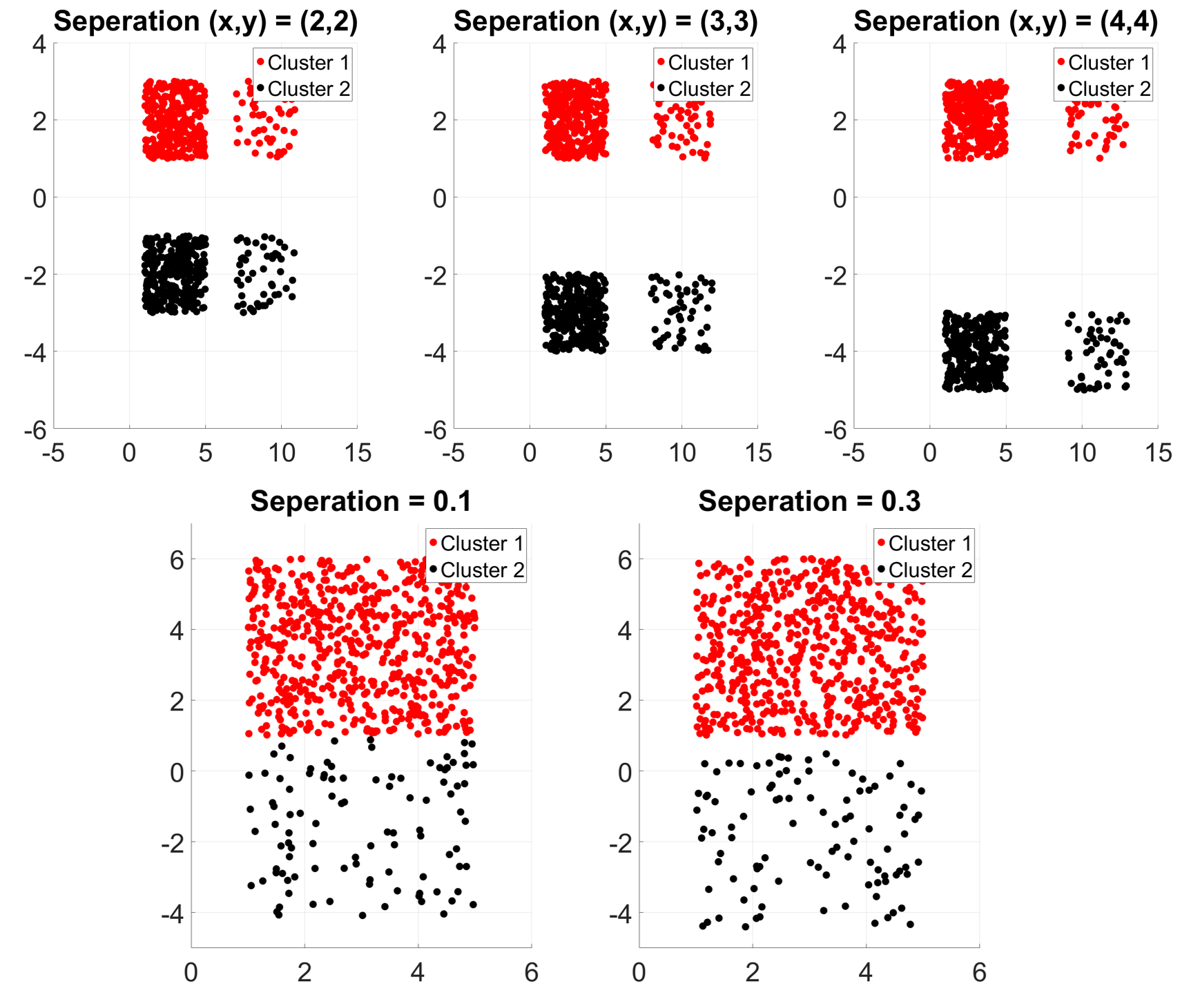
Figure 1: The Balanced and ImBalanced in the two consecutive rows respectively. They comprise two clusters (red/black) with an increasing separation between clusters.

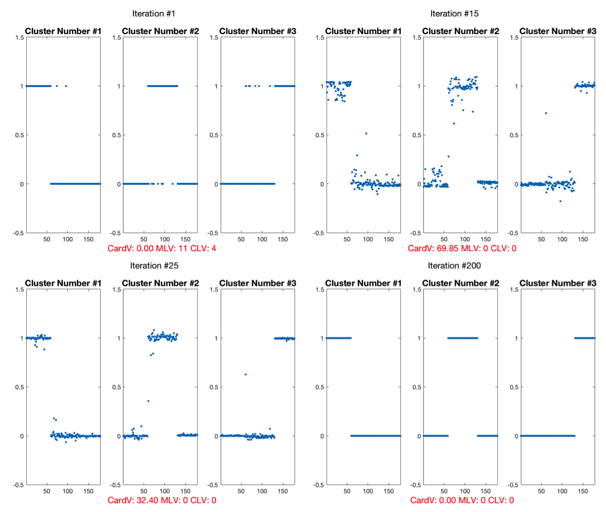
Figure 2: Convergence of the solution $\mathbf{x}$ using $\ell_{p}$Km-Mix with random binary initialization that satisfy the cardinality constraints on the Wine dataset.

TABLE II: Comparison between K-means and $\ell_{p}$Km on real UCI datasets using K-means objective value, ARI(%), MI and HI(%) along with the standard deviation.

Datasets	K-mean (Obj Value)	$\ell_{p}$Km (Obj Value)
wine	195.91 $\pm$ 0.05	195.86 $\pm$ 0.07
iris	29.894 $\pm$ 4.84	28.282 $\pm$ 0.05
glass	81.277 $\pm$ 5.49	85.944 $\pm$ 1.307
	K-means (ARI)	$\ell_{p}$Km (ARI(%))
wine	84.765 $\pm$ 0.92	86.779 $\pm$ 0.10
iris	67.831 $\pm$ 8.79	72.41 $\pm$ 0.90
glass	17.454 $\pm$ 1.31	14.96 $\pm$ 0.91
	K-means (MI)	$\ell_{p}$Km (MI)
wine	0.068 $\pm$ 0.004	0.059 $\pm$ 0.001
iris	0.145 $\pm$ 0.048	0.122 $\pm$ 0.004
glass	0.338 $\pm$ 0.019	0.319 $\pm$ 0.019
	K-means (HI)	$\ell_{p}$Km (HI(%))
wine	86.423 $\pm$ 0.82	88.225 $\pm$ 0.001
iris	70.969 $\pm$ 9.51	75.590 $\pm$ 0.008
glass	32.378 $\pm$ 3.57	36.134 $\pm$ 0.038

TABLE III: Comparison between K-means and $\ell_{p}$Km-Car on synthetic balanced and Imbalaced synthetic datasets using ARI(%), MI and HI(%).

Datasets	K-mean (ARI)	$\ell_{p}$Km-Car (ARI)
Balanced (x,y)=(2,2)	59.97 $\pm$ 51.68	100 $\pm$ 0
Balanced (x,y)=(3,3)	89.99 $\pm$ 31.64	100 $\pm$ 0
Balanced (x,y)=(4,4)	79.99 $\pm$ 42.19	100 $\pm$ 0
Imbalanced y=0.1	34.67 $\pm$ 0	99.46 $\pm$ 0.37
Imbalanced y=0.3	32.26 $\pm$ 0	100 $\pm$ 0
	K-means (MI)	$\ell_{p}$Km-Car (MI)
Balanced (x,y)=(2,2)	0.2003 $\pm$ 0.2586	0 $\pm$ 0
Balanced (x,y)=(3,3)	0.0501 $\pm$ 0.1583	0 $\pm$ 0
Balanced (x,y)=(4,4)	0.1001 $\pm$ 0.2111	0 $\pm$ 0
Imbalanced y=0.1	0.3082 $\pm$ 0	0.002 $\pm$ 0.0014
Imbalanced y=0.3	0.3222 $\pm$ 0	0 $\pm$ 0
	K-means (HI)	$\ell_{p}$Km-Car (HI)
Balanced (x,y)=(2,2)	59.94 $\pm$ 5.171	100 $\pm$ 0
Balanced (x,y)=(3,3)	89.99 $\pm$ 31.67	100 $\pm$ 0
Balanced (x,y)=(4,4)	79.97 $\pm$ 42.22	100 $\pm$ 0
Imbalanced y=0.1	38.35 $\pm$ 0	99.6$\pm$ 0.28
Imbalanced y=0.3	35.57 $\pm$ 0	100 $\pm$ 0

As for the implementation details, none of the selection matrices used in the proposed framework (i.e. $\mathbf{E}_{1},\mathbf{E}_{2},\mathbf{E}_{3},\mathbf{E}_{4},\mathbf{P},\mathbf{C},\mathbf{Q},\Psi,\Lambda_{j}$) are actually constructed. Only element indexing within vectors is used, thus, keeping the necessary computation cost minimal. For ease, all $\rho_{i}$ parameters have the same value and updated similarly. We find that setting all $\rho_{i}$ parameters to 20 and by increasing it it every 5 iterations by 10% for all real datasets achieves the fastest convergence. Moreover, we initialize all the optimization variables using zero vectors, while $\mathbf{x}$ is initialized to random (i.e. random assignment of data points to clusters) if the comparison is against K-means. When comparing against other clustering methods, we use the same K-means initialization as other methods. In all comparisons, $\mathbf{w}$ is initialized to a feasible point as given in Algorithm 1. MATLAB is used to implement our method. The most expensive operation in our framework is the $\mathbf{x}$ and $\mathbf{w}$ updates, which involve solving an $n\times k$ linear system. This is the bottleneck of our framework causing it to have a computational complexity $\mathcal{O}(n^{3}k^{3})$ per iteration. In the final experiment, we report the runtime of our framework on different sized datasets with a variety of constraint choices.

As for the evaluation metric, we adopt the 3 most common criteria used in the clustering community to compare different clustering methods, namely the Adjusted Random Index (ARI)($\nearrow$), Mirkin’s Index (MI) ($\searrow$) and Hubert’s Index (HI) ($\nearrow$) which calculate a measure of agreement between two partitions of a dataset [25, 26]. The symbol $\nearrow$ indicate that the higher the number the better performance and vice versa for $\searrow$. In all experiments, clustering is repeated 10 times with different initializations and we report the average and standard deviation of the metric used in comparison.

2. Comparing Different Constraint Design Choices. We apply our proposed method, $\ell_{p}$Km, on the same clustering task with several choices of constraints: no constraints, only cardinality constraints, only pairwise constraints and both types jointly. We refer to each as $\ell_{p}$Km, $\ell_{p}$Km-Car, $\ell_{p}$Km-Pair and $\ell_{p}$Km-Mix respectively.

(i) An Auxiliary Experiment. Despite that we do not provide a proof for the convergence of the non-quadratic objective in Eq. 1, as it is proven for the quadratic case in [17], we find the performance very stable where we demonstrate it empirically. For instance, we run $\ell_{p}$Km-Mix that enforces cardinality, 20 must-link and 20 cannot-link constraints. In figure 2, we plot the three pieces of the solution label vector $\mathbf{x}$ at four different ADMM iterations (1, 15, 25, and 200). In the first iteration, the initial clustering is random however satisfying the cardinality constraints, so it is binary but it does not lead to a good objective. As ADMM progresses, the continuous solution $\mathbf{x}$ becomes more and more binary, until it converges to a feasible binary solution where the three clusters are disjoint satisfying all constraints. Moreover, we also report the number of cardinality (CardV), must-link (MLV), and cannot-link (CLV) violations at each of these iterations. These violations gradually decrease until convergence occurs, when no violations persist. We find this stable performance across all datasets as will be presented in later sections. Further detailed experiments can be found in the supplementary material.

TABLE IV: Comparison of several pairwise constrained clustering methods against $\ell_{p}$Km-Pair using ARI(%), as well as, must-link (MLV) and cannot-link (CLV) violations in the constraints. The cells indicated with x imply that the underlying method does not attain a feasible solution after 1000 runs.

	Constraints	COP-KMEANS			Spectral Clustering			PPC			CCL			$\ell_{p}$Km-Pair
		ARI($\%$)	MLV	CLV	ARI($\%$)	MLV	CLV	ARI($\%$)	MLV	CLV	ARI($\%$)	MLV	CLV	ARI($\%$)	MLV	CLV
wine
	20ml, 20cl	87.14 $\pm$ 1.06	0	0	91.07 $\pm$ 2	0	0	88.19 $\pm$ 0	1	0	74.52 $\pm$ 0	0	0	91.67 $\pm$ 0	0	0
	40ml, 40cl	84.48 $\pm$ 0.71	0	0	96.67 $\pm$ 0	0	0	89.68 $\pm$ 1.64	1	1.5	53.58 $\pm$ 0	3	4	88.04 $\pm$ 0	0	0
	60ml, 60cl	91.22 $\pm$ 0	0	0	94.87 $\pm$ 0	2	0	89.74 $\pm$ 0.04	4.8	2.9	82.79 $\pm$ 0	7	1	98.32 $\pm$ 0	0	0
	80ml, 80cl	93.09 $\pm$ 0	0	0	96.67 $\pm$ 0	1	0	87.73 $\pm$ 0.74	6	3	55 $\pm$ 0	11	10	94.87 $\pm$ 0	0	0
	100ml, 100cl	96.51 $\pm$ 0	0	0	94.87 $\pm$ 0	3	2	88.33 $\pm$ 0.14	4.4	2.1	90.34 $\pm$ 0	1	5	96.51 $\pm$ 0	0	0
iris
	20ml, 20cl	69.57 $\pm$ 0.61	0	0	80.27 $\pm$ 0.64	1.1	2.2	90.39 $\pm$ 0	1	0	68.28 $\pm$ 0	0	2	72.87 $\pm$ 0	0	0
	40ml, 40cl	74.37 $\pm$ 0	0	0	90.38 $\pm$ 0	1	1	92.22 $\pm$ 0	1	2	45.65 $\pm$ 0	3	11	72.76 $\pm$ 0	0	0
	60ml, 60cl	x	x	x	69.00 $\pm$ 0.59	0	19.5	97.99 $\pm$ 0	0	1	54.86 $\pm$ 0	2	0	100 $\pm$ 0	0	0
	80ml, 80cl	x	x	x	68.44 $\pm$ 0	0	20	97.99 $\pm$ 0	0	1	54.17 $\pm$ 0	2	0	100 $\pm$ 0	0	0
	100ml, 100cl	x	x	x	68.44 $\pm$ 0	0	20	97.99 $\pm$ 0	0	1	52.52 $\pm$ 0	4	1	100 $\pm$ 0	0	0

TABLE V: Comparison of several pairwise constrained clustering methods against $\ell_{p}$Km-Pair using MI and HI(%). The cells indicated with x imply that the underlying method does not attain a feasible solution after 1000 runs.

	Constraints	COP-KMEANS		Spectral Clustering		PPC		CCL		$\ell_{p}$Km-Pair
		MI	HI($\%$)	MI	HI($\%$)	MI	HI($\%$)	MI	HI($\%$)	MI	HI($\%$)
wine
	20ml, 20cl	0.06 $\pm$ 0.01	88.55 $\pm$ 0.95	0.04 $\pm$ 0.01	92.03 $\pm$ 1.8	0.05 $\pm$ 0	89.48 $\pm$ 0	0.11 $\pm$ 0	77.32 $\pm$ 0	0.04 $\pm$ 0	92.57 $\pm$ 0
	40ml, 40cl	0.07 $\pm$ 0	86.18 $\pm$ 0.62	0.02 $\pm$ 0	97.03 $\pm$ 0	0.05 $\pm$ 0.02	90.80 $\pm$ 1.46	0.21 $\pm$ 0	57.37 $\pm$ 0	0.05 $\pm$ 0	89.34 $\pm$ 0
	60ml, 60cl	0.04 $\pm$ 0	92.15 $\pm$ 0	0.02 $\pm$ 0	95.42 $\pm$ 0	0.05 $\pm$ 0	90.85 $\pm$ 0.04	0.08 $\pm$ 0	84.69 $\pm$ 0	0.01 $\pm$ 0	98.50 $\pm$ 0
	80ml, 80cl	0.03 $\pm$ 0	93.83 $\pm$ 0	0.02 $\pm$ 0	97.03 $\pm$ 0	0.06 $\pm$ 0	89.07 $\pm$ 0.66	0.20 $\pm$ 0	59.63 $\pm$ 0	0.02 $\pm$ 0	95.42 $\pm$ 0
	100ml, 100cl	0.02 $\pm$ 0	96.88 $\pm$ 0	0.02 $\pm$ 0	95.42 $\pm$ 0	0.05 $\pm$ 0	89.60 $\pm$ 0.13	0.04 $\pm$ 0	91.39 $\pm$ 0	0.02 $\pm$ 0	96.88 $\pm$ 0
iris
	20ml, 20cl	0.14 $\pm$ 0.01	72.92 $\pm$ 0.49	0.09 $\pm$ 0.036	82.41 $\pm$ 5.11	0.04 $\pm$ 0	91.50 $\pm$ 0	0.14 $\pm$ 0	71.36 $\pm$ 0	0.12 $\pm$ 0	75.95 $\pm$ 0
	40ml, 40cl	0.11 $\pm$ 0	77.18 $\pm$ 0.75	0.04 $\pm$ 0	91.50 $\pm$ 0	0.03 $\pm$ 0	93.13 $\pm$ 0	0.26 $\pm$ 0	49.01 $\pm$ 0	0.12 $\pm$ 0	75.95 $\pm$ 0
	60ml, 60cl	x	x	0.14 $\pm$ 0	71.91 $\pm$ 0.58	0.01 $\pm$ 0	98.23 $\pm$ 0	0.22 $\pm$ 0	55.38 $\pm$ 0	0 $\pm$ 0	100 $\pm$ 0
	80ml, 80cl	x	x	0.14 $\pm$ 0	71.36 $\pm$ 0	0.01 $\pm$ 0	98.23 $\pm$ 0	0.22 $\pm$ 0	55.69 $\pm$ 0	0 $\pm$ 0	100 $\pm$ 0
	100ml, 100cl	x	x	0.14 $\pm$ 0	71.36 $\pm$ 0	0.01 $\pm$ 0	98.23 $\pm$ 0	0.23 $\pm$ 0	53.18 $\pm$ 0	0 $\pm$ 0	100 $\pm$ 0

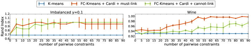
Figure 3: Effect of increasing must-link and cannot-link constraints separately, as compared to unconstrained K-means.

TABLE VI: Comparison of several pairwise constrained clustering methods against $\ell_{p}$Km-Pair using MI and HI(%). The cells indicated with x imply that the underlying method does not attain a feasible solution after 1000 runs.

Datasets

$\ell_{p}$Km-Car

$\ell_{p}$Km-Pair

$\ell_{p}$Km-Mix

ARI($\%$)

MI

HI($\%$)

Time

ARI($\%$)

MI

HI($\%$)

Time

ARI($\%$)

MI($\%$)

HI

Time

ionosphere

8.49 $\pm$ 0

0.46 $\pm$ 0

9.03 $\pm$ 0

1.50 sec

35.65 $\pm$ 0.67

0.321 $\pm$ 0.003

35.68 $\pm$ 0.57

5.00 sec

80.42 $\pm$ 4.35

0.097 $\pm$ 0.002

80.54 $\pm$ 4.32

6.57 sec

Hepatitis

17.12 $\pm$ 1.5

0.36 $\pm$ 0.01

29.07 $\pm$ 1.28

0.55 sec

38.17 $\pm$ 4.01

0.303 $\pm$ 0.021

39.49 $\pm$ 4.33

0.99 sec

46.25 $\pm$ 15.74

0.230 $\pm$ 0.067

54 $\pm$ 13.47

1.09 sec

Hepatitis1

40.98 $\pm$ 7.48

0.24 $\pm$ 0.03

52.86 $\pm$ 5.29

0.91 sec

26.97 $\pm$ 12.26

0.358 $\pm$ 0.065

28.50 $\pm$ 12.96

0.70 sec

77.27 $\pm$ 10.01

0.091 $\pm$ 0.040

81.85 $\pm$ 7.99

1.26 sec

Breast Cancer Wis-D

74.93 $\pm$ 0

0.125 $\pm$ 0

75.03 $\pm$ 0

3.36 sec

74.93 $\pm$ 0

0.128 $\pm$ 0

74.42 $\pm$ 0

3.27 sec

74.93 $\pm$ 0

0.125 $\pm$ 0

75.03 $\pm$ 0

9.27 sec

(i) Traditional K-means versus $\ell_{p}$Km. First, we start by comparing our vanilla constrained free version clustering method $\ell_{p}$Km against K-means. We show that $\ell_{p}$Km method can in fact attain very similar, if not better, performance than traditional K-means (builtin MATLAB function). This is clearly because both methods use the same objective value and that $\ell_{p}$Km does converge to good solutions. Experiments are conducted on some of the UCI datasets [7] (wine, iris and glass). Table II reports the K-means objective value, ARI(%), MI and HI(%) metrics for both methods.

(ii) Traditional K-means versus $\ell_{p}$Km-Car. Here, we demonstrate that our framework coupled with only cardinality constraints outperforms traditional unconstrained K-means on a variety of synthetic data. This highlights the importance of having this prior information available and harnessing it in the clustering process. In these experiments, the cardinality constraints are generated from ground truth labels. To show that cardinality does in fact help clustering performance, we apply $\ell_{p}$Km-Car on the two synthetic datasets (Balanced and ImBalanced) and report their ARI, MI and HI results in Table III.

For the Balanced dataset, the separation between the four groups of points increases. In fact, K-means tends to cluster points together such that each cluster has a similar variance as other clusters. Consequently, K-means clusters the high-density points of the Balanced dataset together and groups the remaining less dense points into another cluster. In comparison, our framework exploits the cardinality constraints to achieve perfect clustering performance. Similarly, the ImBalanced dataset contains two imbalanced clusters with very different densities, where the separation between them is increased. In this case, K-means often mixes data points between clusters, since the cardinality constraints are not used. On the other hand, $\ell_{p}$Km-Car can almost perfectly predict the ground truth clustering labels. Interestingly, the variance of our results is much lower than that of K-means even though they both use the same clustering initialization. This indicates that the cardinality constraints afford our method robustness to the initialization.

To the best of our knowledge, all previous work that handles generic cardinality constraints do not have readily available code for comparison. Therefore, we only compare our method with traditional unconstrained K-means, so as to demonstrate the effectiveness of adding cardinality constraints to an unconstrained clustering method.

(iii) Pairwise Constrained Clustering Methods versus $\ell_{p}$Km-Pair. Here, we compare our $\ell_{p}$Km-Pair method against several pairwise constrained methods from the literature, namely Constrained Clustering [13] (COP-KMEANS), Spectral Clustering [8], Penalized probabilistic Clustering (PPC) [10] and CCL [11]. All pairwise constraints were randomly generated. Among these methods, only COP-KMEANS [13] and $\ell_{p}$Km-Pair exactly enforce the constraints, while the others incorporate them as soft pairwise constraints in their clustering framework. Consequently, Spectral Clustering, PPC and CCL may result in clustering violations. However, due to the heuristic nature of COPKMEANS, it may lead to a situation where depending on the initialization no feasible solution is attained. We run all five methods on two UCI datasets (wine, iris) and ensure that all methods receive the same randomly generated pairwise constraints. Tables IV and V report the performance of these methods on all discussed metrics. For each experiment, we also report the number of must-link (ml) and cannot-link (cl) constraints, as well as, the number of must-link violations (MLV) and the cannot-link violations (CLV). It is clear that $\ell_{p}$Km-Pair outperforms all other methods, while satisfying all the constraints.

(iv) K-means versus $\ell_{p}$Km-Mix. Here, we demonstrate the main motivation behind our flexible framework, namely its ability to incorporate both cardinality and pairwise constraints simultaneously in the clustering optimization. Firstly, and following previous work [13], we demonstrate that increasing the number of pairwise constraints (either must-link or cannot-link) with the same cardinality constraints consistently improves performance. We conduct this experiment on two different datasets: one synthetic (ImBalanced y=0.1) and one real (wine). Figure 3 compares our method against traditional K-means in such setup. Obviously, K-means does not benefit from the constraints while ours consistently improves in performance. Secondly, we compare all three variants of our framework, i.e. cardinality only constraints ($\ell_{p}$Km-Car), pairwise only constraints ($\ell_{p}$Km-Pair) and both ($\ell_{p}$Km-Mix), on several UCI datasets (ionosphere, Hepatitis, Hepatitis1 and Breast Cancer Wis-D). The number of must-link and cannot-link constraints were equal for each dataset and they were set proportional to the dataset size to (20,25,20,100) respectively. Results in Table VI show that our method performs increasingly and significantly better, when more constraint categories are used simultaneously. This improvement reaches as high as 40$\%$ in ARI for some datasets. We also report in table VI the runtime for all 3 different varients on all 4 datasets. The time vary depending on the dataset size and the number of clusters from $0.5-10$ seconds. We did not compare against other methods here, since there is no existing work that combines both categories of constraints in a unified framework and extending the pairwise constrained methods to cardinality constraints is not trivial.

V Conclusion

We proposed a new flexible framework to handle both pairwise and cardinality constraints for K-means clustering. The resulting integer program is transformed into an equivalent continuous reformulation where pairwise constraints are incorporated as quadratic constraints. The resultant problem is solved using ADMM. Extensive experiments have been conducted on both synthetic and real datasets to demonstrate the competitive performance of our method under different constraint choices and that the proposed method achieves state-of-art performance when both types of constraints are used simultaneously. As a future work, we seek to adapt our work to deep clustering approaches [27, 28, 29], which jointly learn feature representations and cluster assignments. That is to say, the ADMM updates will involove another minimization step that trains the encoder for the feature learning procedure while the other steps involve on sloving both the assignment and imposing the constraints. This shall have applications in biology, medicine, finance, and animation, as in many such applications, where pseudo labales in terms of assignments are provided as constraints, e.g., two patients are labeled to have a similar syndrome, feature learning will allow for further improvements in clustering performance.

VI Appendix

Reformulation of Constrained K-means.

We start with our formulation of constrained K-means in Equation (1) below (or Equation (4) in the manuscript).

$$\min_{\mathbf{x},\mathbf{w},\mathbf{z}_{1},\mathbf{z}_{2},\mathbf{z}_{3},\mathbf{z}_{4}}\sum_{j=1}^{k}\sum_{i=1}^{n}x_{ij}\left\|\mathbf{s}_{i}-\mathbf{S}\Lambda_{j}\mathbf{w}\right\|_{2}^{2}$$

$$\text{s.t.}\Psi^{\top}\mathbf{x}=\mathbf{1}_{n},\mathbf{z}_{1}\in S_{b},\mathbf{z}_{2}\in S_{2},\mathbf{Q}\mathbf{P}^{\top}\mathbf{x}=\mathbf{u},$$

$$\mathbf{x}=\mathbf{P}\mathbf{w}\odot\mathbf{C}\mathbf{x},\left(\mathbf{E}_{1}\mathbf{z}_{3}\right)^{\top}\mathbf{E}_{2}\mathbf{x}=v,\left(\mathbf{E}_{3}\mathbf{z}_{4}\right)^{\top}\mathbf{E}_{4}\mathbf{x}=0,$$

$$\mathbf{x}=\mathbf{z}_{1},\mathbf{x}=\mathbf{z}_{2},\mathbf{x}=\mathbf{z}_{3},\mathbf{x}=\mathbf{z}_{4}.$$

We define $\mathbf{X}\in\mathbb{R}^{k\times n}$ and therefore $\mathbf{x}=\text{vect}(\mathbf{X})$. The vect operator simply vectorizes the matrix one column at a time (i.e. one data point at a time). The order of concatenation is reverse for the label vector: $\mathbf{w}=\text{vect}(\mathbf{W})$, where $\mathbf{W}\in\mathbb{R}^{n\times k}$ (i.e. the vectorization is done one cluster at a time). Therefore, it is important to point out that the order of the binary labels $\mathbf{x}$ and that of $\mathbf{w}$ is swapped. Reordering these vectors based on data points or clusters is controlled by the permutation matrix $\mathbf{P}\in\mathbb{R}^{nk\times nk}$. Therefore, $\mathbf{P}\mathbf{x}=\mathbf{P}^{\top}\mathbf{x}=\text{vect}(\mathbf{X}^{\top})$ and $\mathbf{P}\mathbf{w}=\mathbf{P^{\top}}\mathbf{w}=\text{vect}(\mathbf{W}^{\top})$. Throughout the main manuscript and the appendix, we use $\mathbf{P}$ and $\mathbf{P}^{\top}$ to change the order of w to the same order as $\mathbf{x}$ and vice versa. Matrix $\mathbf{S}\in\mathbb{R}^{d\times n}$ in Equation (1) simply concatenates all the data points in its columns, where $\Lambda_{j}\in\mathbb{R}^{n\times nk}$ is zero everywhere except for the $\text{j}^{\text{th}}$ block that is identity, i.e. $\Lambda_{j}=\begin{bmatrix}=\mathbf{0},\dots,\mathbf{I}_{k}^{j},\dots\end{bmatrix}$.

As for $\Psi^{\top}\in\mathbb{R}^{n\times nk}$, it is a binary matrix that has in each row a vector $\mathbf{1}_{k}^{\top}$ that sums all the binary labels for a given data point while the rest are zeros. We write this matrix in blockwise form as follows:

$$\Psi^{\top}=\begin{bmatrix}\mathbf{1}_{k}^{\top}&\mathbf{0}_{k}&\cdots\\ \mathbf{0}_{k}^{\top}&\mathbf{1}_{k}^{\top}&\mathbf{0}_{k}\\ \vdots&\vdots&\vdots\\ \mathbf{0}_{k}&\cdots&\mathbf{1}_{k}\end{bmatrix}$$

As for $\mathbf{Q}\in\mathbb{R}^{k\times nk}$, it sums all the binary labels of each cluster at a time for all the data points and its blockwise matrix form is given as follows:

$$\mathbf{Q}=\begin{bmatrix}\mathbf{1}_{n}^{T}&\mathbf{0}_{nk-n}^{T}&\ldots&\\ \mathbf{0}_{n}^{T}&\mathbf{1}_{n}^{T}&\mathbf{0}_{nk-n}^{T}&\cdots\\ &\cdots&\cdots&&\end{bmatrix}$$

As for $\mathbf{C}\in\mathbb{R}^{nk\times nk}$, it sums the binary labels for each cluster at a time and its blockwise matrix form is as follows:

$$\mathbf{C}=\begin{bmatrix}\mathbf{I}_{k}&\cdots&\mathbf{I}_{k}\\ \vdots&\cdots&\vdots\\ \mathbf{I}_{k}&\cdots&\mathbf{I}_{k}\end{bmatrix}$$

As for the box and $\ell_{2}$-sphere constraints (which intersects with the binary vector space), we define two sets: $S_{b}:=$ $\{\mathbf{a}:\mathbf{0}\leq\mathbf{a}\leq\mathbf{1}\}$ and $S_{2}:=\left\{\mathbf{a}\in\mathbb{R}^{n}:\left\|\mathbf{a}-\frac{1}{2}\mathbf{1}\right\|_{2}^{2}=\frac{n}{2}\right\}$, respectively. It is shown in [17] that: $\{0,1\}^{n}=S_{b}\cap S_{2}$.

Lastly, $\mathbf{E}_{1},\mathbf{E}_{2}\in\mathbb{R}^{kv\times nk}$ and $\mathbf{E}_{3},\mathbf{E}_{4}\in\mathbb{R}^{ke\times nk}$ are selection matrices for the must-link and cannot-link constraints respectively. They select the data points that are involved in both types of constraints.

Applying ADMM. Following the conventional treatment of an optimization problem using ADMM, we first formulate the augmented Lagrangian function is given as follows:

$$\mathcal{L}\left(\mathbf{x},\mathbf{w},\mathbf{z}_{1},\mathbf{z}_{2},\mathbf{z}_{3},\mathbf{z}_{4},\mathbf{y}_{1},\mathbf{y}_{2},\mathbf{y}_{3},\mathbf{y}_{4},\mathbf{y}_{5},y_{6},\mathbf{y}_{7},y_{8},\mathbf{y}_{9}\right):=$$

$$\sum_{j=1}^{k}\sum_{i=1}^{n}x_{ij}\left\|\mathbf{s}_{i}-\mathbf{S}\Lambda_{j}\mathbf{w}\right\|_{2}^{2}+\mathbf{y}_{1}^{\top}\left(\Psi^{\top}\mathbf{x}-\mathbf{1}_{n}\right)+\frac{\rho_{1}}{2}\left\|\Psi^{\top}\mathbf{x}-\mathbf{1}_{n}\right\|_{2}^{2}+$$

$$\mathbb{I}_{\left\{\mathbf{z}_{1}\in S_{b}\right\}}+\mathbf{y}_{2}^{\top}\left(\mathbf{x}-\mathbf{z}_{1}\right)+\frac{\rho_{2}}{2}\left\|\mathbf{x}-\mathbf{z}_{1}\right\|_{2}^{2}+\mathbb{I}_{\left\{\mathbf{z}_{2}\in S_{2}\right\}}+\mathbf{y}_{3}^{\top}\left(\mathbf{x}-\mathbf{z}_{2}\right)+$$

$$\frac{\rho_{3}}{2}\left\|\mathbf{x}-\mathbf{z}_{2}\right\|_{2}^{2}+\mathbf{y}_{4}^{\top}\left(\mathbf{Q}\mathbf{P}^{\top}\mathbf{x}-\mathbf{u}\right)+\frac{\rho_{4}}{2}\left\|\mathbf{QP}^{\top}\mathbf{x}-\mathbf{u}\right\|_{2}^{2}+$$

$$\mathbf{y}_{5}^{\top}\left(\mathbf{I}-\operatorname{diag}(\mathbf{Pw})\mathbf{C}\right)\mathbf{x}+\frac{\rho_{5}}{2}\|\left(\mathbf{I}-\operatorname{diag}(\mathbf{Pw})\mathbf{C}\right)\mathbf{x}\|_{2}^{2}+$$

$$y_{6}\left(\mathbf{z}_{3}^{\top}\mathbf{E}_{1}^{\top}\mathbf{E}_{2}\mathbf{x}-v\right)+\frac{\rho_{6}}{2}\left\|\mathbf{z}_{3}^{\top}\mathbf{E}_{1}^{\top}\mathbf{E}_{2}\mathbf{x}-v\right\|_{2}^{2}+\mathbf{y}_{7}^{\top}\left(\mathbf{x}-\mathbf{z}_{3}\right)+$$

$$\frac{\rho_{7}}{2}\left\|\mathbf{x}-\mathbf{z}_{3}\right\|_{2}^{2}+y_{8}\left(\mathbf{z}_{4}^{\top}\mathbf{E}_{3}^{\top}\mathbf{E}_{4}\mathbf{x}\right)+\frac{\rho_{8}}{2}\left\|\mathbf{z}_{4}^{\top}\mathbf{E}_{3}^{\top}\mathbf{E}_{4}\mathbf{x}\right\|_{2}^{2}+$$

$$\mathbf{y}_{9}^{\top}\left(\mathbf{x}-\mathbf{z}_{4}\right)+\frac{\rho_{9}}{2}\left\|\mathbf{x}-\mathbf{z}_{4}\right\|_{2}^{2}.$$

ADMM updates steps tend to update each primal variable ( $\mathbf{x},\mathbf{w}$, and $\mathbf{z}_{1-4}$ sequentially, while keeping the rest of these variables and the dual variables $\mathbf{y}_{1-5},\mathbf{y}_{6,8}$, and $\mathbf{y}_{6,9})$ set to their most recent values. After the primal variables are updated, the dual variables are updated via a single gradient ascent step. Next, we detail each update step and the underlying optimization sub-problem that needs to be solved.

Update $\mathbf{x}$:

$$\mathbf{x}\leftarrow\underset{\mathbf{x}}{\arg\min}\sum_{j=1}^{k}\sum_{i=1}^{n}x_{ij}\left\|\mathbf{s}_{\mathbf{i}}-\mathbf{S}\Lambda_{j}\mathbf{w}\right\|_{2}^{2}+\mathbf{y}_{1}^{\top}\left(\Psi^{\top}\mathbf{x}-\mathbf{1}_{n}\right)+$$

$$\frac{\rho_{1}}{2}\left\|\Psi^{\top}\mathbf{x}-\mathbf{1}_{n}\right\|_{2}^{2}+\mathbf{y}_{2}^{\top}\left(\mathbf{x}-\mathbf{z}_{1}\right)+\frac{\rho_{2}}{2}\left\|\mathbf{x}-\mathbf{z}_{1}\right\|_{2}^{2}+\mathbf{y}_{3}^{\top}\left(\mathbf{x}-\mathbf{z}_{2}\right)+$$

$$\frac{\rho_{3}}{2}\left\|\mathbf{x}-\mathbf{z}_{2}\right\|_{2}^{2}+\mathbf{y}_{4}^{\top}\left(\mathbf{Q}\mathbf{P}^{\top}\mathbf{x}-\mathbf{u}\right)+\frac{\rho_{4}}{2}\left\|\mathbf{Q}\mathbf{P}^{\top}\mathbf{x}-\mathbf{u}\right\|_{2}^{2}+$$

$$\mathbf{y}_{5}^{\top}(\mathbf{I}-\operatorname{diag}(\mathbf{P}\mathbf{w})\mathbf{C})\mathbf{x}+\frac{\rho_{5}}{2}\|(\mathbf{I}-\operatorname{diag}(\mathbf{P}\mathbf{w})\mathbf{C})\mathbf{x}\|_{2}^{2}+$$

$$y_{6}\left(\mathbf{z}_{4}^{\top}\mathbf{E}_{1}^{\top}\mathbf{E}_{2}\mathbf{x}-v\right)+\frac{\rho_{6}}{2}\left\|\mathbf{z}_{4}^{\top}\mathbf{E}_{1}^{\top}\mathbf{E}_{2}\mathbf{x}-v\right\|_{2}^{2}+\mathbf{y}_{7}^{\top}\left(\mathbf{x}-\mathbf{z}_{4}\right)+$$

$$\frac{\rho_{7}}{2}\left\|\mathbf{x}-\mathbf{z}_{4}\right\|_{2}^{2}+y_{8}\left(\mathbf{z}_{5}^{\top}\mathbf{E}_{3}^{\top}\mathbf{E}_{4}\mathbf{x}\right)+\frac{\rho_{8}}{2}\left\|\mathbf{z}_{5}^{\top}\mathbf{E}_{3}^{\top}\mathbf{E}_{4}\mathbf{x}\right\|_{2}^{2}+\mathbf{y}_{9}^{\top}\left(\mathbf{x}-\mathbf{z}_{5}\right)+$$

$$\frac{\rho_{9}}{2}\left\|\mathbf{x}-\mathbf{z}_{5}\right\|_{2}^{2}$$

The aforemention problem is strongly convex quadratic in $\mathbf{x}$. Therefore, a stationary point is necessary and sufficient for optimality. By equating the gradient to zero, we get:

$$\Big{(}\rho_{1}\Psi\Psi^{\top}+\left(\rho_{2}+\rho_{3}+\rho_{7}+\rho_{9}\right)\mathbf{I}_{nk}+\rho_{4}\mathbf{P}\mathbf{Q}^{\top}\mathbf{Q}\mathbf{P}^{\top}+$$

$$\rho_{5}(\mathbf{I}-\operatorname{diag}(\mathbf{P}\mathbf{w})\mathbf{C})^{\top}(\mathbf{I}-\operatorname{diag}(\mathbf{P}\mathbf{w})\mathbf{C})+$$

$$\rho_{6}\mathbf{E}_{2}^{\top}\mathbf{E}_{1}\mathbf{z}_{3}\mathbf{z}_{3}^{\top}\mathbf{E}_{1}^{\top}\mathbf{E}_{2}+\rho_{8}\mathbf{E}_{4}^{\top}\mathbf{E}_{4}\mathbf{z}_{4}\mathbf{z}_{5}^{\top}\mathbf{E}_{3}^{\top}\mathbf{E}_{4}\Big{)}\mathbf{x}=$$

$$-\left(\operatorname{vect}(\mathbf{B})+\Psi\mathbf{y}_{1}+\mathbf{y}_{2}+\mathbf{y}_{3}-\rho_{1}\Psi\mathbf{1}_{n}-\rho_{2}\mathbf{z}_{1}-\right.$$

$$\rho_{3}\mathbf{z}_{2}-\mathbf{C}^{\top}\operatorname{diag}(\mathbf{P}\mathbf{w})\mathbf{y}_{5}+y_{6}\mathbf{E}_{2}^{\top}\mathbf{E}_{1}\mathbf{z}_{4}-\rho_{6}v\mathbf{E}_{2}^{\top}\mathbf{E}_{1}\mathbf{z}_{3}+\mathbf{y}_{7}-$$

$$\left.\rho_{7}\mathbf{z}_{3}+y_{8}\mathbf{E}_{4}^{\top}\mathbf{E}_{3}\mathbf{z}_{4}+\mathbf{y}_{9}-\rho_{9}\mathbf{z}_{4}+\mathbf{P}\mathbf{Q}^{\top}\mathbf{y}_{4}-\rho_{4}\mathbf{P}\mathbf{Q}^{\top}\mathbf{u}\right),$$

where $\mathbf{B}(i,j)=\left\|\mathbf{s}_{\mathbf{i}}-\mathbf{S}\Lambda_{j}\mathbf{w}\right\|_{2}^{2}$.

Update $\mathbf{w}$:

$$\mathbf{w}\leftarrow\underset{\mathbf{w}}{\arg\min}\sum_{j=1}^{k}\sum_{i=1}^{n}x_{ij}\left\|\mathbf{s}_{\mathbf{i}}-\mathbf{S}\Lambda_{j}\mathbf{w}\right\|_{2}^{2}+$$

$$\mathbf{y}_{5}^{T}(\mathbf{I}-\operatorname{diag}(\mathbf{P}\mathbf{w})\mathbf{C})\mathbf{x}+\frac{\rho_{5}}{2}\left\|(\mathbf{I}-\operatorname{diag}(\mathbf{P}\mathbf{w})\mathbf{C})\mathbf{x}\right\|_{2}^{2}.$$

Similarly to the $\mathrm{x}$-update, the problem is strongly convex quadratic and finding a stationary point is necessary and sufficient for a global solution. Thus, the gradient is given by:

$$-\sum_{j=1}^{k}\sum_{i=1}^{n}2x_{ij}\left(\mathbf{S}\Lambda_{j}\right)^{T}\left(\mathbf{s}_{i}-\mathbf{S}\Lambda_{j}\mathbf{w}\right)-\mathbf{P}^{T}\mathbf{C}\mathbf{x}\odot\mathbf{y}_{5}-$$

$$\rho_{5}\left(\mathbf{P}^{T}\operatorname{diag}(\mathbf{C}\mathbf{x})\right)(\mathbf{I}-\operatorname{diag}(\mathbf{P}\mathbf{w})\mathbf{C})\mathbf{x}=0.$$

Then, we have

$$-\sum_{j=1}^{k}\sum_{i=1}^{n}2x_{ij}\Lambda_{j}^{T}\mathbf{S}^{T}\mathbf{s}_{i}+\sum_{j=1}^{k}\sum_{i=1}^{n}2x_{ij}\Lambda_{j}^{T}\mathbf{S}^{T}\mathbf{S}\Lambda_{j}\mathbf{w}-\mathbf{P}^{T}\mathbf{Cx}\odot\mathbf{y}_{5}$$

$$-\rho_{5}\mathbf{P}^{T}\mathbf{C}\mathbf{x}\odot\mathbf{x}+\rho_{5}\mathbf{P}^{T}\operatorname{diag}(\mathbf{Cx})\operatorname{diag}(\mathbf{P}\mathbf{w})\mathbf{C}\mathbf{x}=0.$$

Therefore,

$$\left[\sum_{j=1}^{k}\sum_{i=1}^{n}2x_{ij}\Lambda_{j}^{T}\mathbf{S}^{T}\mathbf{S}\Lambda_{j}\mathbf{w}+\rho_{5}\mathbf{P}^{T}\operatorname{diag}(\mathbf{C}\mathbf{x})\operatorname{diag}(\mathbf{P}\mathbf{w})\mathbf{C}\mathbf{x}\right]$$

$$=\sum_{j}^{k}\sum_{i}^{n}2x_{ij}\Lambda_{j}^{T}\mathbf{S}^{T}\mathbf{s}_{i}+\mathbf{P}^{T}\mathbf{C}\mathbf{x}\odot\mathbf{y}_{5}+\rho_{5}\mathbf{P}^{T}\mathbf{Cx}\odot\mathbf{x}$$

Finally, we have,

$${\left[\sum_{j=1}^{k}\sum_{i=1}^{n}2x_{ij}\Lambda_{j}^{T}\mathbf{S}^{T}\mathbf{S}\Lambda_{j}+\rho_{5}\mathbf{P}^{T}\operatorname{diag}(\mathbf{C}\mathbf{x}\odot\mathbf{C}\mathbf{x})\mathbf{P}\right]\mathbf{w}}$$

$$=\sum_{j=1}^{k}\sum_{i=1}^{n}2x_{ij}\Lambda_{j}^{T}\mathbf{S}^{T}\mathbf{s}_{i}+\mathbf{P}^{T}\mathbf{C}\mathbf{x}\odot\mathbf{y}_{5}+\rho_{5}\mathbf{P}^{T}\mathbf{C}\mathbf{x}\odot\mathbf{x}$$

In this derivation, we use the fact that $\nabla_{\mathbf{w}}\left(\mathbf{y}_{5}^{T}\mathbf{P}\mathbf{w}\odot\right.$ $\mathbf{Cx})=\mathbf{P}^{T}\mathbf{C}\mathbf{x}\odot\mathbf{y}_{5}$. Tp see why this is the case, note the following identities: $\mathbf{a}\odot\mathbf{b}=\mathbf{b}\odot\mathbf{a}=\operatorname{diag}(\mathbf{a})\mathbf{b}=$ $\operatorname{diag}(\mathbf{b})\mathbf{a}$.

Therefore,

$$\nabla_{\mathbf{w}}\left(\mathbf{y}_{5}^{T}\mathbf{P}\mathbf{w}\odot\mathbf{C}\mathbf{x}\right) =\nabla_{\mathbf{w}}\left(\mathbf{y}_{5}^{T}\operatorname{diag}(\mathbf{C}\mathbf{x})\mathbf{P}\mathbf{w}\right)$$

$$=\mathbf{P}^{T}\operatorname{diag}(\mathbf{C}\mathbf{x})\mathbf{y}_{5}$$

$$=\mathbf{P}^{T}\mathbf{C}\mathbf{x}\odot\mathbf{y}_{5}$$

Update $\mathbf{z}_{1}$:

$$\mathbf{z}_{1}\leftarrow\underset{\mathbf{z}_{1}\in S_{b}}{\arg\min}\mathbf{y}_{2}^{\top}\left(\mathbf{x}-\mathbf{z}_{1}\right)+\frac{\rho_{2}}{2}\left\|\mathbf{x}-\mathbf{z}_{1}\right\|_{2}^{2}$$

$$\mathbf{z}_{1}\leftarrow\underset{\mathbf{z}_{1}\in S_{b}}{\arg\min}\left\|\mathbf{z}_{1}-\left(\mathbf{x}+\frac{\mathbf{y}_{2}}{\rho_{2}}\right)\right\|_{2}^{2}$$

$$\mathbf{z}_{1}=\mathbf{P}_{S_{b}}\left(\mathbf{x}+\frac{\mathbf{y}_{2}}{\rho_{2}}\right)$$

Here, we need to perform a simple projection onto the box set $S_{b}$. The projection $\mathbf{P}_{S_{b}}(.)$ is an elementwise clamping between 0 and $+1$ that is, $\mathbf{P}_{S_{b}}(a)=\min(\max(a,0),1)$ for a scalar value $a$.

Update $\mathbf{z}_{2}$:

$$\mathbf{z}_{2}\leftarrow\underset{\mathbf{z}_{2}\in S_{2}}{\arg\min}\mathbf{y}_{3}^{\top}\left(\mathbf{x}-\mathbf{z}_{2}\right)+\frac{\rho_{3}}{2}\left\|\mathbf{x}-\mathbf{z}_{2}\right\|_{2}^{2}$$

$$\mathbf{z}_{2}\leftarrow\underset{\mathbf{z}_{2}\in S_{2}}{\arg\min}\left\|\mathbf{z}_{2}-\left(\mathbf{x}+\frac{\mathbf{y}_{3}}{\rho_{3}}\right)\right\|_{2}^{2}$$

$$\mathbf{z}_{2}=\mathbf{P}_{S_{2}}\left(\mathbf{x}+\frac{\mathbf{y}_{3}}{\rho_{3}}\right)$$

We need to perform a simple projection onto the $\ell_{2^{-}}$ sphere: $S_{2}=\left\{\mathbf{a}\in\mathbb{R}^{n}:\left\|\mathbf{a}-\frac{1}{2}\mathbf{1}\right\|_{2}^{2}=\frac{n}{4}\right\}$. The projection $\mathbf{P}_{\mathcal{S}_{2}}(.)$ (.) involves an elementwise shift and $\ell_{2}$ vector normalization and thus is given as $\mathbf{P}_{\mathcal{S}_{2}}(\mathbf{a})=\frac{\sqrt{n}}{2}\left(\frac{\mathbf{a}-\frac{1}{2}\mathbf{1}}{\left\|\mathbf{a}-\frac{1}{2}\mathbf{1}\right\|_{2}}\right)+\frac{1}{2}\mathbf{1}$, for any vector $\mathbf{a}\in\mathbb{R}^{n}$.

Update $\mathbf{z}_{3}$:

$$\mathbf{z}_{3}\leftarrow\underset{\mathbf{z}_{3}}{\text{argmin}}~{}~{}y_{6}(\mathbf{z}_{3}^{\top}\mathbf{E}_{1}^{\top}\mathbf{E}_{2}\mathbf{x})+\frac{\rho_{6}}{2}\left\|\mathbf{z}_{3}^{\top}\mathbf{E}_{1}^{\top}\mathbf{E}_{2}\mathbf{x}-v\right\|_{2}^{2}-\mathbf{y}_{7}^{\top}\mathbf{z}_{3}+$$

$$\frac{\rho_{7}}{2}\left\|\mathbf{x}-\mathbf{z}_{3}\right\|_{2}^{2}$$

The problem is strongly convex quadratic in $\mathbf{z}_{4}$, so we obtain the unique global minimizer by equating the gradient to zero as follows

$${\left[\rho_{6}\mathbf{E}_{1}^{\top}\mathbf{E}_{2}\mathbf{x}\mathbf{x}^{\top}\mathbf{E}_{2}^{\top}\mathbf{E}_{1}+\rho_{7}\mathbf{I}_{nk}\right]\mathbf{z}_{4}=\mathbf{y}_{7}+\rho_{7}\mathbf{x}-y_{6}\mathbf{E}_{1}^{\top}\mathbf{E}_{2}\mathbf{x+}}$$

$$\rho_{6}v\mathbf{E}_{1}^{\top}\mathbf{E}_{2}\mathbf{x}$$

Update $\mathbf{z}_{4}$:

$$\mathbf{z}_{4}\leftarrow\underset{\mathbf{z}_{4}}{\text{argmin}}~{}~{}y_{8}(\mathbf{z}_{4}^{\top}\mathbf{E}_{3}^{\top}\mathbf{E}_{4}\mathbf{x})+\frac{\rho_{8}}{2}\left\|\mathbf{z}_{4}^{\top}\mathbf{E}_{3}^{\top}\mathbf{E}_{4}\mathbf{x}\right\|_{2}^{2}-\mathbf{y}_{9}^{\top}\mathbf{z}_{4}+$$

$$\frac{\rho_{9}}{2}\left\|\mathbf{x}-\mathbf{z}_{4}\right\|_{2}^{2}$$

The problem is also strongly convex quadratic in $\mathbf{z}_{5}$, so we obtain the unique global minimizer by equating the gradient to zero as follows

$$\left[\rho_{8}\mathbf{E}_{3}^{\top}\mathbf{E}_{4}\mathbf{x}\mathbf{x}^{\top}\mathbf{E}_{4}^{\top}\mathbf{E}_{3}+\rho_{9}\mathbf{I}_{nk}\right]\mathbf{z}_{5}=\mathbf{y}_{9}+\rho_{9}\mathbf{x}-y_{8}\mathbf{E}_{3}^{\top}\mathbf{E}_{4}\mathbf{x}$$

Update $\mathbf{y}_{1},\mathbf{y}_{2},\mathbf{y}_{3},\mathbf{y}_{4},\mathbf{y}_{5},y_{6},\mathbf{y}_{7},y_{8},\mathbf{y}_{9}$: Lastly, we need to perform dual gradient ascent to update the dual variables as follows:

$$\mathbf{y}_{1}\leftarrow\mathbf{y}_{1}+\rho_{1}\left(\Psi^{\top}\mathbf{x}-\mathbf{1}_{n}\right),\quad\mathbf{y}_{2}\leftarrow\mathbf{y}_{2}+\rho_{2}\left(\mathbf{x}-\mathbf{z}_{2}\right)$$

$$\mathbf{y}_{3}\leftarrow\mathbf{y}_{3}+\rho_{3}\left(\mathbf{x}-\mathbf{z}_{3}\right),\quad\mathbf{y}_{4}\leftarrow\mathbf{y}_{4}+\rho_{4}\left(\mathbf{QP}^{\top}\mathbf{x}-\mathbf{u}\right)$$

$$\mathbf{y}_{5}\leftarrow\mathbf{y}_{5}+\rho_{5}(\mathbf{x}-\mathbf{Pw}\odot\mathbf{Cx}),\quad y_{6}\leftarrow y_{6}+\rho_{6}\left(\mathbf{z}_{3}^{\top}\mathbf{E}_{1}^{\top}\right.$$

$$\mathbf{y}_{7}\leftarrow\mathbf{y}_{7}+\rho_{7}\left(\mathbf{x}-\mathbf{z}_{3}\right),\quad y_{8}\leftarrow y_{8}+\rho_{8}\left(\mathbf{z}_{4}^{\top}\mathbf{E}_{3}^{\top}\mathbf{E}_{4}\mathbf{x}\right)$$

$$\mathbf{y}_{9}\leftarrow\mathbf{y}_{9}+\rho_{9}\left(\mathbf{x}-\mathbf{z}_{4}\right)$$

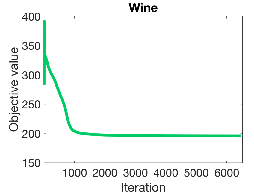
Figure 4: Convergence of the K-means objective value us- ing FCKm with random initialization on the Wine dataset. Note the decreasing nature of the objective and its smooth convergence to the solution

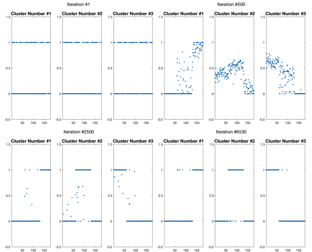
Figure 5: Convergence of the solution x using FCKm with random initialization on the Wine dataset.

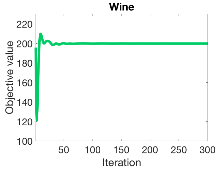
Figure 6: Convergence of the K-means objective value using FCKm-Mix with a random initialization on Wine dataset.

VII Auxiliary Results

We present some additional experimental results that augment the discussion made in the manuscript. Primarily, we provide empirical evidence that our FCKm method and its constrained variants converge to binary solutions that satisfy different constraints (pairwise and cardinality).

Convergence for Unconstrained Clustering. In Figure 4, we plot the K-means objective value at each ADMM iteration for an unconstrained clustering task with three clusters. Note that the initialization to this problem is a random threeway clustering. The objective decreases monotonically (after the first 2-3 iterations) and converges to a minimum value in approximately 6000 iterations. The optimization is stable with no perturbations at the onset of convergence.

In Figure 5, we plot the cluster vector for each of the three clusters being optimized at different iterations $(1,500,2500$, and 6530), i.e. we plot the three pieces of the label vector $\mathrm{x}$. In the first iteration, the initial clustering is done randomly, so it is binary but it does not lead to a good objective. As ADMM progresses, the continuous solution $\mathrm{x}$ becomes more and more binary, until it converges to a feasible binary solution where the three clusters are completely disjoint.

Convergence for Constrained Clustering. In Figure 6, we plot the K-means objective value at each ADMM iteration for a constrained clustering task with three clusters. In this task, we enforce cardinality, must-link, and cannotlink constraints onto the optimization. The initialization is taken to be a random assignment between the three disjoint clusters. In this case, the objective tends to be monotonically increasing after the first few iterations. This might seem counter-intuitive, since we are trying to minimize the objective. However, it must be noted that the continuous solution vector $\mathbf{x}$ in each ADMM iteration tends not to be feasible with respect to the enforced constraints. In other words, these constraints are being enforces more and more as the ADMM process proceeds, which forces the tradeoff between objective and feasibility. But, similar to the unconstrained case, the variation in objective is smooth and no perturbations are exhibited when ADMM begins to converge.

Moreover, Figure 4 plots the solution vectors for each cluster at four different iterations $(1,15,25,200)$. A similar behavior to the unconstrained case is encountered, where disjoint binary solution vectors are converged to. However, the notable difference is that we also report the number of cardinality (CardV), must-link (MLV), and cannotlink (CLV) violations at each of these iterations. We see that these violations gradually decrease until convergence occurs, when no violations persist.

References

- [1] G. Karypis, E.-H. Han, and V. Kumar, “Chameleon: Hierarchical clustering using dynamic modeling,” Computer, vol. 32, no. 8, pp. 68–75, 1999.
- [2] B. Wu and B. Hu, “Density and neighbor adaptive information theoretic clustering,” in Neural Networks (IJCNN), The 2011 International Joint Conference on. IEEE, 2011.
- [3] O. Chapelle and A. Zien, “Semi-supervised classification by low density separation.” in AISTATS, 2005, pp. 57–64.
- [4] K. Wagstaff and C. Cardie, “Clustering with instance-level constraints,” AAAI/IAAI, 2000.
- [5] D. Klein, S. D. Kamvar, and C. D. Manning, “From instance-level constraints to space-level constraints: Making the most of prior knowledge in data clustering,” Stanford, Tech. Rep., 2002.
- [6] A. Ng, M. Jordan, and Y. Weiss, “On spectral clustering: Analysis and an algorithm,” Advances in neural information processing systems, vol. 14, 2001.
- [7] P. Bradley, K. Bennett, and A. Demiriz, “Constrained k-means clustering,” Microsoft Research, Redmond, 2000.
- [8] Z. Lu and H. H. Ip, “Constrained spectral clustering via exhaustive and efficient constraint propagation,” in European Conference on Computer Vision. Springer, 2010, pp. 1–14.
- [9] U. Von Luxburg, “A tutorial on spectral clustering,” Statistics and computing, 2007.
- [10] Z. Lu and T. K. Leen, “Penalized probabilistic clustering,” Neural Computation, 2007.
- [11] B.-R. Dai, C.-R. Lin, M.-S. Chen et al., “On the techniques for data clustering with numerical constraints,” Age, 2003.
- [12] B. Wu, Y. Zhang, B.-G. Hu, and Q. Ji, “Constrained clustering and its application to face clustering in videos,” in Proceedings of the IEEE Conference on Computer Vision and Pattern Recognition, 2013.
- [13] K. Wagstaff, C. Cardie, S. Rogers, S. Schrödl et al., “Constrained k-means clustering with background knowledge,” in ICML, vol. 1, 2001, pp. 577–584.
- [14] F. Hoppner and F. Klawonn, “Clustering with size constraints,” in Computational Intelligence Paradigms. Springer, 2008, pp. 167–180.
- [15] F. Klawonn and F. Hoppner, “Equi-sized, homogeneous partitioning,” in International Conference on Knowledge-Based and Intelligent Information and Engineering Systems. Springer, 2006.
- [16] J. Shi and J. Malik, “Normalized cuts and image segmentation,” in IEEE Transactions on pattern analysis and machine intelligence. IEEE, 2000.
- [17] B. Wu and B. Ghanem, “lp-box admm: A versatile framework for integer programming,” IEEE transactions on pattern analysis and machine intelligence, 2018.
- [18] D. H. Fisher, “Knowledge acquisition via incremental conceptual clustering,” Machine learning, vol. 2, no. 2, pp. 139–172, 1987.
- [19] S. Basu, M. Bilenko, and R. J. Mooney, “A probabilistic framework for semi-supervised clustering,” in Proceedings of the tenth ACM SIGKDD international conference on Knowledge discovery and data mining. ACM, 2004, pp. 59–68.
- [20] B. Wu, S. Lyu, B.-G. Hu, and Q. Ji, “Simultaneous clustering and tracklet linking for multi-face tracking in videos,” in Proceedings of the IEEE International Conference on Computer Vision, 2013, pp. 2856–2863.
- [21] I. S. Dhillon, Y. Guan, and B. Kulis, A unified view of kernel k-means, spectral clustering and graph cuts. Citeseer, 2004.
- [22] H. Ding and J. Xu, “A unified framework for clustering constrained data without locality property,” in Proceedings of the Twenty-Sixth Annual ACM-SIAM Symposium on Discrete Algorithms. SIAM, 2015.
- [23] K.-C. Duong, C. Vrain et al., “A declarative framework for constrained clustering,” in Joint European Conference on Machine Learning and Knowledge Discovery in Databases. Springer, 2013, pp. 419–434.
- [24] J. Peng and Y. Wei, “Approximating k-means-type clustering via semidefinite programming,” SIAM journal on optimization, 2007.
- [25] L. Hubert and P. Arabie, “Comparing partitions,” Journal of Classification, vol. 2, no. 1, pp. 193–218, Dec 1985. [Online]. Available: https://doi.org/10.1007/BF01908075
- [26] M. Meila, “Comparing clusterings–an information based distance,” Journal of multivariate analysis, vol. 98, no. 5, pp. 873–895, 2007.
- [27] A. Alqahtani, X. Xie, J. Deng, and M. Jones, “A deep convolutional auto-encoder with embedded clustering,” in Proceedings of the IEEE International Conference on Image Processing, 2018, pp. 4058–4062.
- [28] A. Alqahtani, X. Xie, J. Deng, and M. W. Jones, “Learning discriminatory deep clustering models,” in Proceedings of the International Conference on Computer Analysis of Images and Patterns, 2019, pp. 224–233.
- [29] A. Alqahtani, M. Ali, X. Xie, and M. W. Jones, “Deep time-series clustering: A review,” Electronics, vol. 10, no. 23, p. 3001, 2021.