An Optimal Algorithm to Solve the Combined Task Allocation and Path Finding Problem

Abstract

We consider multi-agent transport task problems where, e.g. in a factory setting, items have to be delivered from a given start to a goal pose while the delivering robots need to avoid collisions with each other on the floor.

We introduce a Task Conflict-Based Search (TCBS) Algorithm to solve the combined delivery task allocation and multi-agent path planning problem optimally. The problem is known to be NP-hard and the optimal solver cannot scale. However, we introduce it as a baseline to evaluate the sub-optimality of other approaches. We show experimental results that compare our solver with different sub-optimal ones in terms of regret.

I Introduction

In Multi-Agent Path Finding (MAPF) the problem specification assigns a fixed start and goal state to each agent and the core challenge is to find collision free paths for all agents. In contrast, both Multi-Agent Task Allocation (MATA) and Multi-Agent Pick-up and Delivery (MAPD) focus on solving the allocation of delivery jobs to the agents, while collisions between agent paths (e.g. in traffic networks) are not considered an issue. This paper considers the joint problem of delivery task allocation and finding collision free paths for all agents jointly. We denote this as the Combined Task Allocation and Path Finding (CTAPF) problem.

This problem setting is motivated by dense factory floor transportation systems. Here items have to be transported from their current locations to goal locations by robotic agents that share narrow aisles and routes in the factory floor. More generally, the problem setting captures any multi-agent domain where the tasks are to traverse from one state to another, and spatio-temporal constraints between the agents exist.

As our problem setting is a superset of multi-agent path finding, it is NP-hard. In this paper we introduce an explicit optimal solver for such problems, which necessarily cannot scale well with the number of agents. We use the method to evaluate the regret (sub-optimality) of alternative approaches in our experiments.

In section III we introduce the CTAPF problem formulation. We then present in section IV an optimal solver. In section V we show simulation experiments using our algorithm.

II Related Work

The task allocation problem is a well researched challenge in the field of multi-agent systems and operations research. We refer to it as MATA. A centralized approach to solve it is the Hungarian algorithm [1]. Further, there exist auction based approaches allowing to solve the problem decentralized [2]. More recently additional market-based approaches [3], reactive methods [4] or biologically inspired ones [5] have been introduced. We model the problem in a way such that one agent can only perform one task at the time and every task only requires one agent. In the taxonomy by [6] this is an ST-SR-TA problem (Single-Task Robots, Single-Robot Tasks, Time-Extended Assignment) which is proven to be NP-hard [6].

The particular problem of transport task allocation is called Pickup and Delivery Problem (PDP) [7] in operations research. See [8] for a survey article. It is defined by a set of agents and a number of requests of certain amount to be transported from one location to another. The problem is often studied with time windows [9] or to optimize vehicle capacity [10] especially in the Autonomous Guided Vehicle (AGV) domain [11]. Currently we do not consider time windows because they are usually not defined in industrial scenarios. Also, we are concerned with the special case of the PDP where every agent has a capacity of one unit, since this models the scenario best. This may be also referred to as dial-a-ride problem [7].

Multi-Agent Path Finding (MAPF) is another intensively studied problem in multi-agent systems [12]. The decision in MAPF concerns how a number of agents will be traveling to their goal poses without colliding, also an NP-hard problem [13]. The colored pebble problem is comparable since the color of the pebble makes them not interchangeable [14]. Solving the problem with collision avoidance at runtime can lead to deadlocks especially in narrow environments as discussed by [15] and more recently by [16]. Available sub-optimal solutions to the problem include Local Repair A* [17], WHCA* [15] and sampling based approaches like Multi-agent RRT* [18] and ARMO [19]. Optimal solvers are Increasing Cost Tree Search (ICTS) [20] and Conflict-Based Search (CBS) [21]. Our solution is based on the latter, because it can be extended with task-assignment and can then solve the introduced problem optimally. Previously we elaborated CBS with nonuniform costs in an industrial AGV scenario [22].

One problem formulation that is more closely related to transport systems is the Combined Target-Assignment and Path-Finding (TAPF) introduced by Ma and Koenig [23]. It first solves the assignment problem and MAPF problem but not concurrently, so the costs used for task allocation are not the true costs. Instead of single goals we consider the whole transport task allocation.

A different type of problem is studied in vehicle routing with capacities [24], which focuses on the deliveries from one central depot based on certain demands. This is a different problem in the sense that it considers only one origin and additionally considers capacity constraints.

The joint solution of MATA and MAPF, that we are proposing, was previously studied in [25], where the problem is considered as Mixed Integer Linear Programming (MILP) but due to collisions on the single-agent path level we think it should be considered a Mixed Integer Non-Linear Programming (MINLP) Problem. Therefore, the solver proposed by Koes et al. [25] can not solve the problem optimally since it ignores agent-agent collisions.

A similar problem, by taking uncertainties into account, aims at applications in highly dynamic environments [26]. The solution is also sub-optimal because agent-agent collisions are not considered at planning time.

Similar problems have recently also been formulated by Farinelli et al. [27], Ma et al. [28] and Nguyen et al. [29] for domains that do not involve transport tasks as we consider them. Both find interesting sub-optimal solutions for Token Passing with Task Swaps (TPTS) [28], based on Distributed Constraint Optimization Problems [27] and using answer set programming (ASP) [29]. All of these approaches may solve the sub-problems optimally but they do not solve the combined problem optimally. This would require taking the implications that the task assignment makes into the path finding problem and vice versa.

The field of combined task and motion planning [30] is also combining two planning domains but for mobile manipulators. Our algorithm borrows the concept of hierarchical planners and the reaction to planning errors i.e. when no path is found.

In the literature we can find many approaches that go towards solving the problems of MATA and MAPF in interesting settings. Little research is done in combining both which is the core aspect addressed in this paper. To our knowledge it is the first to solve the combined MATA and MAPF problem optimally.

III Problem Formulation

As discussed above, MAPF and MATA have been researched intensively. We now propose a combined problem formulation.

We consider a configuration space $\mathcal{X}$, and $n$ agents with joint configuration state $x=(x_{1},..,x_{n})\in\mathcal{X}^{n}$.

We have a set $t=\{t_{1},t_{2},...,t_{m}\}$ of $m$ tasks, each one consists of a start $x^{s}_{i}$ and a goal $x^{g}_{i}$ configuration, $t_{i}=(x^{s}_{i},x^{g}_{i})\in\mathcal{X}^{2}$.

Once an agent visits a task’s start pose, it is automatically assigned to the task, and we say the task is running. It is fixed to this task and can not be reassigned to another task before reaching its goal.

The problem is to find a minimum duration $T\in\mathbf{N}$ and paths $P_{j}$ of length $T$ for each agent $j$ such that every task is fulfilled. In the following we more formally define the constraints on the path (that they follow a roadmap and do not collide), and when tasks are fulfilled.

Each path $P_{j}=(P_{j}^{0},..,P_{j}^{T})$ is a sequence of $T+1$ configurations, where $P_{j}^{0}\in\mathcal{X}$ is constrained to be the start configuration of agent $j$, and $P_{j}^{t+1}\in\partial(P_{j}^{t})\subseteq\mathcal{X}$ is adjacent to the agents previous configuration $P_{j}^{t}$. Adjacency is defined by a roadmap $\partial(\bullet)$ which, for each $x\in\mathcal{X}$ defines its neighborhood $\partial(x)\subseteq\mathcal{X}$.

Given the set of paths $\{P_{1},..,P_{n}\}$ we require them to be non-colliding, meaning that $\nexists t,j,k:P_{j}^{t}=P_{k}^{t}$. In addition, we also require agent movements to be non-colliding, that is, they must not swap places on the roadmap, $\nexists t,j,k:P_{j}^{t+1}=P_{k}^{t}\wedge P_{j}^{t}=P_{k}^{t+1}$.

Given a path $P_{j}$ of an agent $j$, we can compute the implicit assignment $\tau_{j}^{T}\in\{1,..,m\}$ of agent $j$ to a task $i\in\{1,..,m\}$ at time step $T$. The mapping from $P_{j}$ to $\tau_{j}$ is unique given the rule that a task becomes automatically active if the agent visits its start configuration and ends only when it reaches the task goal. Based on this it is also uniquely defined whether a task $i$ is fulfilled by a path $P_{j}$. Therefore, given all agent paths $P_{j}$ we can evaluate whether all tasks are fulfilled.

In summary, the input to the problem are the agent’s initial configurations $\{P_{1}^{0},..,P_{n}^{0}\}$, the roadmap defined by $\partial(\bullet)$, and the set of tasks $t$. The output is the total time $T$ per task and all agent paths $\{P_{1},..,P_{n}\}$, subject to the path constraints and fulfillment of all tasks. The objective is to minimize $\sum_{i\in(0,..m)}T_{i}$, the sum of duration per tasks until it is fulfilled.

In the evaluation, we use a grid-map as roadmap graph. The approach can work on any roadmap graph that fulfills the property that none of the poses in the graphs vertices are in collision with any other.

Optimality is only guarantied with respect to the chosen roadmap. I. e. the best solution duration is measured based on the number of roadmap edges traveled in that given roadmap. Therefore, the duration in actual time units depends on the length of the edges and speeds of the agents.

IV Optimal Solver

IV-A Concept

Our Task Conflict-Based Search (TCBS) searches on the level of task assignments for all agents. Given a configuration of task assignments and neglecting collision constraints, we can use standard single-agent path finding to compute the corresponding optimal paths that connect the agents configurations to the start and the start to the goal configurations of all assigned tasks. To also account for the path collision constraints we follow the approach of conflict-based search. This introduces additional decision variables in the search tree that represent the “decision” to put an explicit avoid constraint on an agent path. That is, we not only search for task assignments but also avoid configurations that would contain a collision. We will discuss below that this approach does not compromise optimality of the method.

To give a first intuition on how the search tree is built, we describe it briefly before giving the technical description afterwards: If there are no currently running tasks, we start with an empty assignment in the root node. Therefore, at the beginning all tasks and all agents are unassigned. At every node we perform one of the two following types of expansion: a) Iff no collision between agents exists: Add children for all possible combinations of one still unassigned tasks to one agent. This means that the task will be added at the end of the agents task list. b) else (i.e. iff a collision between agents is detected): The expansion adds nodes where the configuration in the roadmap (or the motion between two configurations) is avoided at the time of the collision, one for each colliding agent. See also Figure 1.

IV-B Decision variables

The discrete decision variables define node $s$ of the search tree, where $s.\tau$ defines the tasks assigned to agents and $s.\beta$ contains avoided configurations (or the motion between two configurations).

For each agent $j$, one assignment list $\tau_{j},j\in\{1,...,n\}$ exists. Each assignment list $\tau_{j}=(t_{j0},t_{j1},...)$ defines the sequence of tasks that the agent $j$ has to fulfill in order. Where each list element $t_{jk}\in\{1,...,m\},k\in\mathbf{N}$ references a task.

To establish collision avoidance we define configurations or motions between configurations that an agent avoids at a given time. For each agent $j$, one avoid list $\beta,j\in\{1,...,n\}$ is defined. Each list can contain multiple avoided configurations: $\beta_{j}=(\beta_{j0},\beta_{j1},...)$. And one avoided configuration is defined by either $\beta_{jk}=(x_{\beta},T_{\beta}),k\in\mathbf{N}$, where $x_{\beta}$ is the configuration to be avoided at time $T_{\beta}$. Or $\beta_{j0}=(x_{\beta 0},x_{\beta 1},T_{\beta})$, where the motion between $x_{\beta 0}$ and $x_{\beta 1}$ is avoided at time $T_{\beta}$.

IV-C Search Algorithm

Given the specific problem formulation in section III we can now describe an optimal solver as A* tree search over assignments of these decision variables. We perform this search by using

• Algorithm 1 to expand nodes,

• Algorithm 2 the goal test,

• Algorithm 3 to decide which nodes to expand first and

• Algorithm 4 to determine the cost-so-far function for a node

Figure 1: Example of a TCBS tree for $n=2$, $m=3$. The second level shows the big branching factor which is in this case 6. The leftmost node has for example a configuration, where the first agent executes task 0. In the third displayed level, the assignments are extended further so that the leftmost node indicates a configuration where the first agent would execute task 1 and then 0. In the rightmost node occurs a collision which is solved through avoiding the configuration (here cell 5, 3 at time 6) in the fourth level (red nodes). The last unassigned task 0 is assigned to the first agent which leads to a solution in the left leaf node of the final level.

IV-D Expand

Input: node $s$

1 children = []

2 if collision in $s$ then

3       // for all agents in collision

4       for $j~{}in~{}\textsf{collision}$ do

5             // add avoided configuration (or motion between them) at a certain point in time for agent $j$

6             children $\leftarrow$ children + $(s.\beta_{j}+(x_{\beta},T_{\beta}))$

7      

8else

9       // for all unassigned tasks

10       for $t\notin s.\tau$ do

11             // for all agents

12             for $j$ do

13                   children $\leftarrow$ children + $(s.\tau_{j}+t)$

14            

15      

16return children

17

Algorithm 1 Expand

In the tree search we use algorithm 1 to expand a node. Figure 1 shows how a search tree after multiple expansions may look like. It is especially visible how the two different types of expansion shape the tree. The blue nodes are added by an assignment expansion while the red ones are added to resolve a collision.

IV-E Goal Test

Input: node $s$

1 // if in collision

2 if collision in $s$ then

3       return false

4// or if unassigned tasks exist

5 else if $\exists t\notin s.\tau$ then

6       return false

7// otherwise it is the goal

8 else

9       return true

10      

11

Algorithm 2 Goal Test

algorithm 2 shows the algorithm to do the goal test that is performed on any evaluated node. It requires the node to have no collisions and all tasks to be assigned.

IV-F Heuristic

Input: node $s$

1 cost = 0

2 // for all unassigned tasks

3 for $t\notin s.\tau$ do

4       cost $\leftarrow$ cost + Distance (closest_agent, start($t$))

5       cost $\leftarrow$ cost + Distance (start($t$), goal($t$))

return cost

Algorithm 3 Heuristic

The heuristic function ($h()$ function of A*) is presented in algorithm 3. It evaluates the cost of the best-possible assignment. This sums for each unsigned task the distance to the closest agent which might be either its starting position or the goal pose of a previously executed task.

IV-G Cost-so-far

Input: node $s$

1 cost = 0

2 // Plan single-agent paths according to assignments and avoided configurations:

3 P $\leftarrow$ getPaths (s) for $p_{x}\in P$ do

4       if $p_{j}\equiv p_{x}$ then

5             // Time at task end added to cost:

6             cost $\leftarrow$ cost + $p_{j}.T_{final}$

7            

8      

9if collisions in $P$ then

10       $s.\textit{{collision}}$ $\leftarrow$ true

d return $s$, cost

Algorithm 4 Cost-so-far

The cost function ($g()$ function of A*) in algorithm 4 evaluates the cost of the node. A sum of all arrival times is used as cost. This method is also used to evaluate if collisions are present in a node by computing the single-agent paths. If a collision is detected, we still calculate costs. It allows for the freedom to solve collision by changing the task assignment which is a benefit of the CTAPF problem formulation.

IV-H Path Function

Our approach requires a function to compute a set of paths for all agents for any given node. This plans single agent paths according to the assigned tasks and the configurations (or motions between two configurations) to be avoided. We also use A* here, but on the environments roadmap. Additionally we cache previously calculated paths to use it multiple times. Both of the presented algorithms (Alg. 3 and Alg. 4) use the notion of $\mathtt{Distance(a,b)}$ which is a method that returns the Manhattan Distance between two points or, if present in the previously mentioned cache, returns the actual distance of the shortest path.

IV-I Optimality

An A* search algorithm is considered optimal if the heuristic function is admissible [31]:

$$h(s)\leq h^{*}(s)~{}\forall~{}s$$ (1)

Where $h(s)$ is the heuristic of node $s$ while $h^{*}(s)$ is the optimal cost.

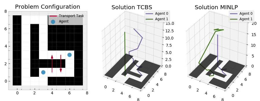
Figure 2: Example problem configuration (left) and solution as path set in space-time (with time as vertical dimension) by our TCBS planner (middle) and by separately solving task allocation as MINLP optimization problem and path finding with CBS (right). For an animated version see video.

The heuristic (algorithm 3) is optimistic since it considers the distance of the closest agent to the tasks goal. This is never greater than the actual path distance:

$$\mathtt{Distance}(closest\_agent,start(task))$$ (2)

$$\leq\mathtt{Path}(assigned\_agent,start(task)).T_{final}$$

Where $T_{final}$ indicates the time at the end of the path assuming constant motion speed.

And for the length of a transport task, the optimality criterion is the same as for single-agent path finding:

$$\mathtt{Distance}(start(task),goal(task))$$ (3)

$$\leq\mathtt{Path}(start(task),goal(task)).T_{final}$$

The methods $\mathtt{Distance(a,b)}$ and $\mathtt{Path(a,b)}$ are described in subsection IV-H in more detail.

The consistency of the heuristic would be required, if we were searching on a general graph with no tree structure [32]. Since algorithm 1 only expands nodes by adding information, the search graph has tree structure and consistency is no required criterion.

That is, our approach adds avoided configurations does not compromise the optimality. The proof is available in the original publication of CBS[21].

V Evaluation

The source code of our implementation in Python is available online.

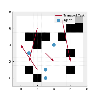
Figure 3: One random configuration that was used for the comparison of different algorithms. Indicating agent locations and transport tasks. Black squares in the background show obstacles.

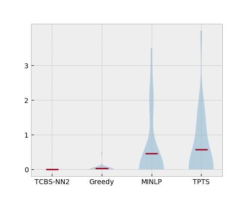
Figure 4: Task duration surplus (i.e. regret) for the indicated algorithms in comparison to the optimal solution of the same problem computed by TCBS. Violin plot with red lines indicating the mean value.

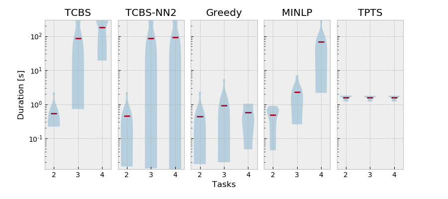
Figure 5: Planning time required by the different algorithms for different problem sizes (i.e. number of tasks). Violin plot with red lines indicating the mean value.

V-A Example Problem and Solution

footnote 2 shows an example of one problem configuration and the resulting path set after solving the problem. We can compare the two solutions by TCBS (middle) and MINLP [25] (right). The algorithms received a set of agent positions and tasks (section III) as input and returned a set of paths for the agents. From the paths in the pictures follow the task execution times displayed in Table I per task. We compare the total time for all tasks $T$, as discussed in section III.

Algorithm	Task 1	Task 2	Total
TCBS	6	15	21
MINLP	6	20	26

TABLE I: Execution times for the tasks in the example.

It is visible that TCBS produces a solution quality superior to MINLP while it does only utilize one agent. The task allocation step of MINLP assigns each agent to the closest task. When the tasks are executed, the two agents in MINLP block each other. In this sense the TCBS algorithm successfully finds a solution that takes the transport task execution into account. This shows how special cases require to jointly solve the MATA and the MAPF problems which is the main claim of this paper.

V-B Algorithms for Comparison

To give further insight into the different sub-optimal solvers we are introducing them in the following before evaluating them afterwards.

• TCBS The optimal planner described in this paper.

• TCBS-NN2 (TCBS for 2 nearest neighbors) A version of our algorithm which uses a sub-optimal nearest-neighbor search [33] to only consider the n (here $n=2$) closest of all possible assignments. Additionally, it uses sub-optimal heuristics to resolve collision faster. It is still not scalable but can find solutions for much bigger problems than TCBS

• Greedy A simple local search algorithm that incrementally assigns tasks to agents using a sub-optimal nearest neighbor search. It finds the currently closest pair of unassigned agents and tasks or tasks and tasks for consecutive execution. See algorithm 5 for details. Then we solve MAPF by the CBS algorithm.

• MINLP The separate solution of assignment and path finding problem proposed by [25] has been implemented using the Bonmin solver [34] for the assignment problem and CBS for path finding.

• TPTS The original goal of this approach is the lifelong version of MAPF. The task assignment is solved in advanced but optimized by swapping of tasks [28]. The implementation was provided by the authors of the paper and is available online.

  Input: agents, tasks

  1 free_agents = agents.copy()

  2free_tasks = tasks.copy()

  3consecutive = dict()

  4agent_task = dict()

  5while len(free_tasks) $>$ 0 do

  6       if len(free_tasks) $>$ len(free_agents) then

  7             poses = free_agents $\cup$ task_ends

  8      else

  9             poses = free_agents

  10      closest_pose, closest_task = nearest_neighbor(poses, free_tasks)

  11      free_tasks.remove(closest_task)

  12      if type(closest_pose) == task then

  13             consec[task] = closest_pose // (task)

  14      else

  15             agent_task[task] = closest_pose

  16            free_agents.remove(closest_pose) // as agent

  17      

  18return consecutive, agent_task

  Algorithm 5 Greedy Assignment

V-C Solution Regret

While the previous example was designed to explicitly show the potential shortcomings of the separate solution of MATA and MAPF problem, we want to focus on a wider comparison of regret for the available approaches now. To allow a more general evaluation, we use now randomized scenarios for this comparison.

This uses a 8x8 map filled with 20% random obstacles each scenario receives 2, 3 or 4 random tasks. Per configuration 30 trials of different random configurations were tested. An example of one randomly generate scenario is shown in Figure 3.

Figure 4 shows the mean value of regret for different solvers. This is, how much more duration per task was required in the respective solution in comparison to the optimal solution. It can be seen from the figure that most planners have a low mean value, meaning they found the optimal solution most of the time. But different planners show different distributions of outliers in the data. No deviation is visible for TCBS-NN2 which is the only algorithm in this comparison that solves MATA and MAPF in combination. It shows that the joint problem solving delivers good overall solution quality (i.e. small regret).

The greedy algorithm shows also a very small regret, demonstrating that also simple approaches can lead to small regret.

Both MINLP and TPTS show the ability to find the optimal solution in the mean case as well but especially TPTS has a significant amount of data with higher regret. This demonstrate that traditional separate solving of MATA and MAPF can lead to a considerable regret.

V-D Planning Time

To compare the algorithms towards their practical usability, we evaluate their planning duration. We used the same random scenarios as introduced before and for this experiment we also differentiate between problem size to elaborate scaling effects in the duration. Problem size is defined as the number of tasks that are introduced.

Figure 5 shows the planning time for the approaches. Compared are all the planners mentioned in subsection V-B It is clearly visible that our TCBS algorithm does not scale well with the problem size. This is due to the problem being NP-hard. The results for TCBS-NN2 show similar scaling effect but also indicate a tendency towards faster computations times for larger problem sizes. This is due to the algorithms pruning of the search tree by nearest neighbor search.

The greedy algorithm shows no visible scaling and fastest mean performance in this comparison. It is very efficient because it always assigns the closest agent.

The MINLP algorithm has a better overall performance than TCBS and TCBS-NN2 but shows exponential scaling as well. This is due to the optimization problems complexity also being NP-hard.

Results for TPTS show good performance and also scales well. The method of task swaps lead to this results because it is independent of the problem size.

Both TPTS and the greedy algorithm could therefore be taken into consideration for practical use although they lack solution quality as seen in the previous experiment.

VI Conclusion

Combined Task Allocation and Path Finding (CTAPF) is a practically highly relevant problem and has, to our knowledge, not been solved optimally previously. We provided a detailed formalization of the problem. The problem can be solved optimally by the proposed Task Conflict-Based Search (TCBS) algorithm based on a dynamically built search-tree. This search-tree incrementally assigns tasks to agents and resolves collisions between agents as they occur. In comparison to other approaches is demonstrated how the combined solving of task allocation and path finding improves the solution quality over solutions that solve them separately. Our optimal algorithm is intended to support the development of sub-optimal planners by evaluating their regret. In addition, we proposed an approximate version of the solver with improved scaling which demonstrates smaller regret than the competing methods.

References

- [1] H. Kuhn, “The Hungarian method of solving the assignment problem,” Nav. Res. Logist. Quart, vol. 2, no. 1-2, pp. 29–47, mar 2010.
- [2] R. Smith, “Communication and Control in Problem Solver,” IEEE Trans. Comput., vol. 29, no. 12, p. 12, dec 1980.
- [3] M. Dias, R. Zlot, N. Kalra, and A. Stentz, “Market-Based Multirobot Coordination: A Survey and Analysis,” Proc. IEEE, vol. 94, no. 7, pp. 1257–1270, jul 2006.
- [4] L. E. Parker, “ALLIANCE: An architecture for fault tolerant multirobot cooperation,” IEEE Trans. Robot. Autom., vol. 14, no. 2, pp. 220–240, 1998.
- [5] C. R. Kube, C. R. Kube, E. Bonabeau, and E. Bonabeau, “Cooperative transport by ant and robots,” Rob. Auton. Syst., vol. 30, p. 37, 1998.
- [6] M. J. Gerkey, Brian P., Mataric, B. Gerkey, and M. Matarić, “A Formal Analysis and Taxonomy of Task Allocation in Multi-Robot Systems,” Int. J. Rob. Res., vol. 23, no. 9, pp. 939–954, 2004.
- [7] M. W. P. Savelsbergh and M. Sol, “The General Pickup and Delivery Problem,” Transp. Sci., vol. 29, no. 1, pp. 17–29, feb 1995.
- [8] S. N. Parragh, K. F. Doerner, and R. F. Hartl, “A survey on pickup and delivery problems. Part I: Transportation between customers and depot,” J. für Betriebswirtschaft, vol. 58, no. 2, pp. 81–117, 2008.
- [9] H. C. Lau and Z. Liang, “Pickup and Delivery with Time Windows : Algorithms and Test Case Generation,” IEEE Comput. Soc. eds, 13th IEEE Int. Conf. Tools with Artif. Intell., pp. 333–340, 2001.
- [10] E. Taniguchi, M. Noritake, T. Yamada, and T. Izumitani, “Optimal size and location planning of public logistics terminals,” Transp. Res. Part E Logist. Transp. Rev., vol. 35, no. 3, pp. 207–222, 1999.
- [11] D. Sinriech and J. M. A. Tanchoco, “Intersection graph method for AGV flow path design,” Int. J. Prod. Res., vol. 29, no. 9, pp. 1725–1732, 1991.
- [12] J. F. Allen, “Maintaining knowledge about temproal intervals,” Readings Qual. Reason. about Phys. Syst., vol. 26, no. 11, pp. 361–372, nov 1990.
- [13] J. Yu and S. LaValle, “Structure and intractability of optimal multi-robot path planning on graphs,” Proc. AAAI Natl. Conf. …, pp. 1443–1449, 2013.
- [14] G. Goraly and R. Hassin, “Multi-color pebble motion on graphs,” Algorithmica (New York), vol. 58, no. 3, pp. 610–636, 2010.
- [15] D. Silver, “Cooperative Pathfinding.” AIIDE, 2005.
- [16] M. Cap, J. Gregoire, and E. Frazzoli, “Provably safe and deadlock-free execution of multi-robot plans under delaying disturbances,” in 2016 IEEE/RSJ Int. Conf. Intell. Robot. Syst., vol. 2016-Novem. IEEE, oct 2016, pp. 5113–5118.
- [17] A. Zelinsky, “A Mobile Robot Exploration Algorithm,” IEEE Trans. Robot. Autom., vol. 8, no. 6, pp. 707–717, 1992.
- [18] M. Cáp and P. Novák, “Multi-agent RRT *: Sampling-based Cooperative Pathfinding,” in Proc. 2013 Int. Conf. Auton. agents multi-agent Syst., 2013, pp. 1263–1264.
- [19] A. Kleiner, D. Sun, A. Kleiner, D. Sun, and D. Meyer-delius, “ARMO - Adaptive Road Map Optimization for Large Robot Teams,” in IEEE/RSJ Int. Conf. Intell. Robot. Syst. (IROS), 2011, 2011, pp. 3276–3282.
- [20] G. Sharon, R. Stern, M. Goldenberg, and A. Felner, “The increasing cost tree search for optimal multi-agent pathfinding,” Artif. Intell., vol. 195, pp. 470–495, 2013.
- [21] G. Sharon, R. Stern, A. Felner, and N. N. R. Sturtevant, “Conflict-based search for optimal multi-agent pathfinding,” Artif. Intell., vol. 219, pp. 40–66, 2015.
- [22] J. Abbenseth, F. G. Lopez, C. Henkel, and S. Dörr, “Cloud-Based Cooperative Navigation for Mobile Service Robots in Dynamic Industrial Environments,” in 32nd ACM SIGAPP Symp. Appl. Comput., 2017.
- [23] H. Ma and S. Koenig, “Optimal Target Assignment and Path Finding for Teams of Agents,” Aamas 2016, pp. 1144–1152, dec 2016.
- [24] M. A. Russell and G. B. Lamont, “A Genetic Algorithm for Unmanned Aerial Vehicle Routing,” in GECCO ’05 Proc. 7th Annu. Conf. Genet. Evol. Comput., 2005, pp. 1523–1530.
- [25] M. Koes, I. Nourbakhsh, K. Sycara, S. D. Ramchurn, and Others, “Heterogeneous multirobot coordination with spatial and temporal constraints,” in Proc. Natl. Conf. Artif. Intell., vol. 20, no. 3, 2005, p. 1292.
- [26] B. Woosley and P. Dasgupta, “Multirobot Task Allocation with Real-Time Path Planning,” Proc. Twenty-Sixth Int. Florida Artif. Intell. Res. Soc. Conf. (FLAIRS-26 Conf. St. Pete Beach, FL, USA, vol. 2224, p. 574579, 2013.
- [27] A. Farinelli, E. Zanotto, and E. Pagello, “Advanced approaches for multi-robot coordination in logistic scenarios,” Rob. Auton. Syst., 2016.
- [28] H. Ma, J. Li, T. K. S. Kumar, and S. Koenig, “Lifelong Multi-Agent Path Finding for Online Pickup and Delivery Tasks,” Proc. 16th Int. Conf. Auton. Agents Multiagent Syst. (AAMAS 2017), no. June, pp. 837–845, may 2017.
- [29] V. Nguyen, P. Obermeier, T. C. Son, T. Schaub, and W. Yeoh, “Generalized Target Assignment and Path Finding Using Answer Set Programming,” in Proc. Twenty-Sixth Int. Jt. Conf. Artif. Intell. California: International Joint Conferences on Artificial Intelligence Organization, aug 2017, pp. 1216–1223.
- [30] J. Wolfe, B. Marthi, and S. Russell, “Combined Task and Motion Planning for Mobile Manipulation.” ICAPS, 2010.
- [31] J. Pearl, Heuristics : intelligent search strategies for computer problem solving. Addison-Wesley Pub. Co, 1984.
- [32] S. J. Russell, P. Norvig, and E. Davis, Artificial intelligence : a modern approach. Prentice Hall, 2010.
- [33] M. Muja and D. G. Lowe, “Scalable nearest neighbor algorithms for high dimensional data,” IEEE Trans. Pattern Anal. Mach. Intell., vol. 36, no. 11, pp. 2227–2240, nov 2014.
- [34] P. Bonami, L. T. Biegler, A. R. Conn, G. Cornuéjols, I. E. Grossmann, C. D. Laird, J. Lee, A. Lodi, F. Margot, N. Sawaya, and A. Wächter, “An Algorithmic Framework for Convex Mixed Integer Nonlinear Programs An algorithmic framework for convex mixed integer nonlinear programs,” Tech. Rep., 2005.