Abstract

Numerical solution of the chemical master equation for stochastic reaction networks typically suffers from the state space explosion problem due to the curse of dimensionality and from stiffness due to multiple time scales. The dimension of the state space equals the number of molecular species involved in the reaction network and the size of the system of differential equations equals the number of states in the corresponding continuous-time Markov chain, which is usually enormously huge and often even infinite. Thus, efficient numerical solution approaches must be able to handle huge, possibly infinite and stiff systems of differential equations efficiently. We present an approximate numerical integration approach that combines a dynamical state space truncation procedure with efficient numerical integration schemes for systems of ordinary differential equations including adaptive step size selection based on local error estimates. The efficiency and accuracy is demonstrated by numerical examples.

1 Introduction

The chemical master equation (CME) describes the random dynamics of many stochastic reaction networks in physics, biology, and chemistry, amongst other sciences. More specifically, many biochemical reaction networks can be appropriately modeled by multivariate continuous-time Markov chains (CTMCs), also referred to as Markov jump processes, where at any time the system state is represented by a vector of the numbers of each molecular species present in the reaction network and the CME is a system of differential equations whose solution, given an initial probability distribution, provides the transient (time-dependent) state probabilities.

Exact analytical solutions of the CME are only available for very small reaction networks or special cases such as, e.g., monomolecular reactions or reversible bimolecular reactions [26, 29]. Therefore, in general computational approaches are required. However, because reaction rates typically differ by several orders of magnitude, the system dynamics possess multiple time scales and the corresponding equations are stiff. Furthermore, the size of the state space typically increases exponentially with the model dimensionality, that is, with the number of molecular species in the reaction network. This effect is often referred to as the curse of dimensionality or state space explosion. Stochastic simulation of the reaction network and the numerical solution of the CME are two common complementary approaches to analyze stochastic reaction networks governed by the CME, both of which must be properly designed to cope with huge, potentially infinite multidimensional state spaces, and stiffness.

Stochastic simulation does not solve the CME directly but imitates the reaction network dynamics by generating trajectories (sample paths) of the underlying CTMC, where a stochastically exact imitation is in principle straightforward [3, 16, 17]. Several mathematically equivalent implementations have been developed [10, 15, 30, 34, 48]. Stochastic simulation does not suffer from state space explosion, because the state space needs not be explicitly enumerated, but in particular stochastic simulation of stiff systems becomes exceedingly slow and inefficient, because simulating all successive reactions in order to generate trajectories of the underlying CTMC advances only in extremely small time steps. In order to tackle this problem approximate stochastic simulation techniques for accelerated trajectory generation have been developed, in particular various tau-leaping methods [1, 8, 9, 19, 43, 44, 50, 53, 56] where, instead of simulating every reaction, at any time $t$ a time step size $\tau$ is determined by which the simulation is advanced.

A general problem of stochastic simulation, however, remains also with approximate techniques: stochastic simulation constitutes an algorithmic statistical estimation procedure that tends to be computationally expensive and only provides estimates whose reliability and statistical accuracy in terms of relative errors or confidence interval half widths depend on the variance of the corresponding simulation estimator. Estimating the whole probability distribution by stochastic simulation is enormously time consuming. Therefore, often only statistical estimates of the expected numbers of molecules are considered, which requires less effort, but in any case, when estimating expectations, probabilities, or any other relevant system property, many stochastically independent and identically distributed trajectories must be generated in order to achieve a reasonable statistical accuracy [49]. Hence, stochastic simulation is inherently costly. In many application domains it is sometimes even referred to as a method of last resort.

Several hybrid approximation approaches combine stochastic simulation with deterministic numerical computations. One way to do this is by distinguishing between low molecular counts, where the evolution is described by the CME and handled by stochastic simulation, and high molecular counts, where an approximation of the CME by the continuous-state Fokker-Planck equation is viable [24, 46]. Another way is to consider time scale separations where parts of the system (states or reactions) are classified as either slow or fast and the different parts are handled by different stochastic simulation approaches and numerical solution techniques [5, 14, 22, 23, 31, 32, 42, 47, 55], or even without resorting to stochastic simulation for any part [6, 51]. As a major drawback, however, for time scale separation methods it is in general hard to define what is slow or fast. In fact, many systems possess multiple time scales rather than only two and a clear separation of time scales is impossible.

Some numerical approximation approaches tackle the state space explosion problem by restricting the analysis of the model to certain subsets of states where the truncated part of the state space has only a sufficiently small probability. For instance, finite state projection (FSP) algorithms [4, 39, 40] consider finite parts of the state space that can be reached either during the whole time period of interest or during multiple time intervals into which the time period of interest is split. Then the computation of transient probabilities is conducted based on the representation of the transient probability distribution as the product of the initial probability distribution times a matrix exponential involving the generator matrix of the underlying CTMC restricted to the finite projection. However, computing matrix exponentials is well known to be an intricate issue in itself [37, 38] and with FSP algorithms it must be repeated multiple times, corresponding to repeated expansions of the finite state projection. Alternative state space truncation methods are based on adaptive wavelet methods [25, 27], or on a conversion to discrete time where it is dynamically decided which states to consider at a certain time step in a uniformized discrete-time Markov chain [2, 33].

While examples show that these methods can handle the state space explosion in some cases, for many systems they are still not feasible, because even the considered finite part of the state space is too large, or because the specific system dynamics hamper the computational methods involved. In particular, even if the state space is relatively small or can be reduced to a manageable size, the stiffness problem must be handled satisfactorily and it is not clear whether these methods are suitable for stiff systems.

In this paper, we present a novel numerical approximation method that tackles both the state space explosion problem and the stiffness problem where we consider efficient approximate numerical integration based on the fact that the CME can be cast in the form of a system of ordinary differential equations (ODEs) and the computation of transient probabilities, given an initial probability distribution, is an initial value problem (IVP). We combine a dynamical state space truncation procedure, efficient numerical integration schemes, and an adaptive step size selection based on local error estimates. The dynamical state space truncation keeps the number of considered states manageable while incurring only a small approximation error. It is much more flexible and can reduce the state space much more than the aforementioned methods. The use of efficient ODE solvers with adaptive step size control ensures that the method is fast and numerically stable by taking as large as possible steps without degrading the method’s convergence order.

Our method approximates the solution of the CME by truncating large, possibly infinite state spaces dynamically in an iterative fashion. At a particular time instant $t$, we consider an approximation of the transient probability distribution and temporarily neglect states with a probability smaller than a threshold $\delta$, that is, their probability at time $t$ is set to zero. The CME is then solved for an (adaptively chosen) time step $h$ during which the truncated state space is adapted to the probability distribution at time $t+h$. More precisely, certain states that do not belong to the truncated part of the state space at time $t$ are added at time $t+h$, when in the meantime they receive a significant amount of probability which exceeds $\delta$. Other states whose probabilities drop below $\delta$ are temporarily neglected. The smaller the significance threshold $\delta$ is chosen the more accurate the approximation becomes.

The dynamical state space truncation approach combined with a 4th-order 4-stage explicit Runge-Kutta integration scheme was applied in [35, 36] to the computation of certain transient rare event probabilities in nonstiff models. The step size at each step was chosen heuristically according to the smallest expected sojourn time in any of the significant states, without any local error control. This works well for nonstiff models, but stiff models require more sophisticated adaptive step size selection strategies based on local error estimates and often even implicit integration schemes [7, 20, 21, 52].

In the present paper we substantially generalize and improve our previous work. We extend the dynamical state space truncation to work for the whole class of Runge-Kutta methods, explicit and implicit, each of which can be equipped with an adaptive step size selection based on local error estimates. This yields an accurate, numerically stable and computationally efficient framework for the approximate solution of the CME for stochastic reaction networks with extremely huge, possibly infinite, multidimensional state spaces.

In the next section we introduce the notation for stochastic reaction networks, the underlying CTMC and in particular the CME that describes the transient probability distribution. Section 3 describes the dynamical state space truncation, its efficient implementation for general Runge-Kutta methods, and the adaptive step size selection based on local error estimates. Examples are provided in Section 4. Finally, Section 5 concludes the paper and outlines further research directions.

2 Chemical Master Equation

Consider a well-stirred mixture of $d\in{\mathbb{N}}$ molecular species $S_{1},\ldots,S_{d}$ in a thermally equilibrated system of fixed volume, interacting through $M\in{\mathbb{N}}$ different types of chemical reactions, also referred to as chemical reaction channels, $R_{1},\ldots,R_{M}$. At any time $t\geq 0$ a discrete random variable $X_{k}(t)$ describes the number of molecules of species $S_{k}$ and the system state is given by the random vector $X(t)=(X_{1}(t),\ldots,X_{d}(t))$.

The system changes its state due to one of the possible reactions, where each reaction channel $R_{m},m=1,\ldots,M$, is defined by a stoichiometric equation

$$R_{m}:\ s_{m_{1}}S_{m_{1}}+\cdots+s_{m_{r}}S_{m_{r}}\stackrel{{\scriptstyle c_{m}}}{{\longrightarrow}}s_{m_{r+1}}S_{m_{r+1}}+\cdots+s_{m_{\ell}}S_{m_{\ell}}$$ (1)

with an associated stochastic reaction rate constant $c_{m},$ reactants $S_{m_{1}},\ldots,S_{m_{r}},$ products $S_{m_{r+1}},\ldots,S_{m_{\ell}},$ and the corresponding stoichiometric coefficients $s_{m_{1}},\ldots,s_{m_{\ell}}\in\mathbb{N},$ where $m_{1},\ldots,m_{\ell}$ indexes those species that are involved in the reaction. Mathematically, the stoichiometry is described by the state change vector $v_{m}=(v_{m1},\ldots,v_{md}),$ where $v_{mk}$ is the change of molecules of species $S_{k}$ due to $R_{m}.$ That is, if a reaction of type $R_{m}$ occurs when the system is in state $x,$ then the next state is $x+v_{m},$ or, equivalently, state $x$ is reached, if a reaction of type $R_{m}$ occurs when the system is in state $x-v_{m}.$

For each reaction channel $R_{m}$ the reaction rate is given by a state-dependent propensity function $\alpha_{m},$ where $\alpha_{m}(x)dt$ is the conditional probability that a reaction of type $R_{m}$ occurs in the time interval $[t,t+dt),$ given that the system is in state $x$ at time $t.$ That is

$$\alpha_{m}(x)dt=P\left(\mbox{$R_{m}$ occurs in}\ [t,t+dt)\ |\ X(t)=x\right).$$ (2)

The propensity function is given by $c_{m}$ times the number of possible combinations of the required reactants and thus computes as

$$\alpha_{m}(x)=c_{m}\prod_{j=1}^{m_{r}}{x_{m_{j}}\choose s_{m_{j}}},$$ (3)

where $x_{m_{j}}$ is the number of molecules of species $S_{m_{j}}$ present in state $x$, and $s_{m_{j}}$ is the stoichiometric coefficient of $S_{m_{j}}$ according to (1). Because at any time the system’s future evolution only depends on the current state, $(X(t))_{t\geq 0}$ is a time-homogeneous continuous-time Markov chain (CTMC), also referred to as a Markov jump process, with $d$-dimensional state space ${\cal X}\subseteq{\mathbb{N}}^{d}$. Since the state space is countable it is always possible to map it to $\mathbb{N}$, which yields a numbering of the states.

The conditional transient (time-dependent) probability that the system is in state $x\in{\cal X}$ at time $t,$ given that the system starts in an initial state $x_{0}\in{\cal X}$ at time $t_{0},$ is denoted by

$$p_{x}(t):=p(x,t):=p(x,t|x_{0},t_{0})=P\left(X(t)=x\ |\ X(t_{0})=x_{0}\right)$$ (4)

and the transient probability distribution at time $t$ is the collection of all transient state probabilities at that time, represented by the row vector $p(t)$. The system dynamics in terms of the state probabilities’ time derivatives are described by the chemical master equation (CME)

$$\frac{\partial p(x,t)}{\partial t}=\sum_{m=1}^{M}\left(\alpha_{m}(x-v_{m})p(x-v_{m},t)-\alpha_{m}(x)p(x,t)\right)=:\mathcal{A}p(t)(x),$$ (5)

which is also well known as the system of Kolmogorov forward differential equations for Markov processes [54]. These stochastic reaction kinetics are physically well justified since they are evidently in accordance with the theory of thermodynamics [18, 54]. In the thermodynamic limit the stochastic description converges to classical deterministic mass action kinetics [28].

Note that (5) is the most common way to write the CME, namely as a partial differential equation (PDE), where $t$ as well as $x_{1},\ldots,x_{d}$ are variables. However, for any fixed state $x=(x_{1},\ldots,x_{d})$ the only free parameter is the time parameter $t$ such that (5) with fixed $x$ is an ordinary differential equation (ODE) with variable $t$. In particular, when solving for the transient state probabilities numerical ODE solvers can be applied. We shall therefore use the notation $p_{x}(t)$ in the following.

3 Approximate Numerical Integration of the CME

Numerical integration methods for solving the CME, given $p^{(0)}:=p(t_{0})$, discretize the integration interval $[0,T]$ and successively compute approximations $p^{(1)}\approx p(t_{1}),p^{(2)}\approx p(t_{2}),\ldots,p^{(\eta)}\approx p(t_{\eta})$, where $0=t_{0}<t_{1}<t_{2}\cdots<t_{\eta}=T$ are the mesh points and $h_{i}=t_{i+1}-t_{i}$ is the step size at the $i$-th step, $i=0,\ldots,{\eta-1}$. With single-step methods each approximation $p^{(i+1)}\approx p(t_{i+1})$ is computed in terms of the previous approximation $p^{(i)}$ only, that is, without using approximations $p^{(j)},j<i$. For advanced methods the step sizes $h_{i}$ (and thus $\eta$, the number of steps) are not determined in advance, but variable step sizes are determined in the course of the iteration.

The system of ODEs described by the CME (5) is typically large or even infinite, because there is one ODE for each state in the underlying CTMC, that is, the size of the system of ODEs equals the size of the CTMC’s state space. Thus, its solution with standard numerical integration methods becomes computationally infeasible. However, one can exploit that at any time only a tractable number of states have “significant” probability, that is, only relatively few states have a probability that is greater than a small threshold.

The main idea of our dynamical state space truncation for numerical integration methods is to integrate only those differential equations in the CME (5) that correspond to significant states. All other state probabilities are (temporarily) set to zero. This reduces the computational effort significantly since in each iteration step only a comparatively small subset of states is considered. Based on the fixed probability threshold $\delta>0$, we dynamically decide which states to drop or add, respectively. Due to the regular structure of the CTMC the approximation error of the algorithm remains small since probability mass is usually concentrated at certain parts of the state space. The farther away a state is from a “significant set” the smaller is its probability. Thus, in most cases the total error of the approximation remains small. Since in each iteration step probability mass may be “lost” the approximation error at step $i$ is the sum of all probability mass lost (provided that the numerical integration could be performed without any errors), that is,

$$1-\sum_{x\in{\cal S}}p_{x}^{(i)}.$$ (6)

It is important to note that other than static state space truncation approaches our dynamical approach allows that in the course of the computation states can “come and go”, that is, states join the significant set if and only if their current probability is above the threshold $\delta$ and states in the significant set are dropped immediately when their current probability falls below $\delta$. Furthermore, states that have previously been dropped may come back, that is they are re-considered as significant as soon as they receive a probability that exceeds the threshold $\delta$. This is substantially different from state space exploration techniques where only the most probable states are generated but states are never dropped as time progresses like for instance in [12] with regard to approximating stationary distributions. Our dynamical state space truncation approach is also much more flexible than finite state projection (FSP) algorithms [4, 39, 40] which work over pre-defined time intervals with the same subset of states, where in particular for stiff systems many reactions can occur during any time interval, so that in order to safely meet reasonable accuracy requirements the resulting subset of states is often still extremely large. In contrast to that we update our set of significant states in each adaptively chosen time step, without much overhead. Furthermore, by numerically integrating the ODEs we avoid the intricate computation of matrix exponentials required in FSP algorithms and by using an efficient data structure we do not even need to generate any matrices.

In order to avoid the explicit construction of a matrix and in order to work with a dynamic set $\mathit{Sig}$ of significant states that changes in each step, we use for a state $x$ a data structure with the following components:

• fields $x.\mathit{p}$, $x.\mathit{p_{2}}$ for the approximated probabilities $p^{(i)}_{x}$ and $p^{(i+1)}_{x}$, respectively,

• for all $m$ with $\alpha_{m}(x)>0$ a pointer to the successor state $x+v_{m}$ as well as a field with the rate $\alpha_{m}(x)$.

Algorithm 1 A numerical adaptive step size integration scheme.

1:$\mathit{Sig}$ $\leftarrow$ $\{x:p_{x}(0)>\delta\}$

2:$t$ $\leftarrow$ 0, $i$ $\leftarrow$ 0

3:compute $h_{0}$

4:while $t<T$ do

5:     compute $p^{(i+1)}$

6:     compute $\hat{\epsilon}_{i}$, $h_{i+1}$

7:     if step successful then

8:         update $\mathit{Sig}$

9:         $t$ $\leftarrow$ $t+h_{i}$, i $\leftarrow$ i+1

10:     end if

11:end while

The workflow of the numerical integration scheme is given in pseudocode in Algorithm 1. We start at time $t=0$ and initialize the set $\mathit{Sig}$ as the set of all states that have initially a probability greater than $\delta$. We compute the initial time step $h_{0}$. In each iteration step we compute the approximation $p^{(i+1)}$ using an explicit or implicit Runge-Kutta method (see Sections 3.1, 3.2). We check whether the iteration step was successful computing the local error estimate $\hat{\epsilon_{i}}$ and ensuring that error tolerance conditions are met. If so, then for each state we update the field $x.\mathit{p}$ with $x.\mathit{p_{2}}$, and remove the state from $\mathit{Sig}$ if its probability becomes less than $\delta$. Based on the local error estimate, we choose a time step for the next iteration (or the repetition of the iteration in case it was not successful). This and the computation of the initial time step is detailed in Section 3.3.

3.1 Runge-Kutta methods

We consider the whole family of Runge-Kutta methods, which proceed each time step of given step size in multiple stages. More precisely, a general $s$-stage Runge-Kutta method proceeds according to the iteration scheme

$$p^{(i+1)}=p^{(i)}+h_{i}\sum_{\ell=1}^{s}b_{\ell}k^{(\ell)},$$ (7)

$$k^{(\ell)}:={\cal A}\left(p^{(i)}+h_{i}\sum_{j=1}^{s}a_{\ell j}k^{(j)}\right),$$ (8)

which is uniquely defined by weights $b_{1}\ldots,b_{s}>0$ with $b_{1}+\cdots+b_{s}=1$ and coefficients $0\leq a_{\ell j}\leq 1$, $\ell=1,\ldots,s,\ j=1,\ldots,s$. Thus, $k^{(\ell)}$ is an approximation to $p(t_{i}+h_{i}c_{\ell})$, where $c_{\ell}=a_{\ell 1}+\cdots+a_{\ell s}$, and $k^{(\ell)}(x)$ is the component of the vector $k^{(\ell)}$ that corresponds to state $x$. Hence, $k^{(\ell)}(x)$ is the probability of $x$ at stage $\ell$. If $a_{\ell j}=0$ for all $j\geq\ell$, then the sum in Equation (8) effectively runs only from $1$ to $\ell-1$, which means that for each $\ell=1,\ldots,s$ the computation of $k^{(\ell)}$ includes only previous stage terms $k^{(j)},j<\ell$. Therefore, $k^{(1)},\ldots,k^{(s)}$ can be computed sequentially, that is, $a_{\ell j}=0$ for all $j\geq\ell$ yields explicit integration schemes. If there is at least one $j\geq\ell$ with $a_{\ell j}>0$, then the integration scheme is implicit, which implies that the solution of at least one linear system of equations is required per iteration step.

Algorithm 2 A single iteration step of a general explicit $s$-stage Runge-Kutta scheme, defined by $s,b_{1},\ldots,b_{s}$, and $a_{\ell j}$ for $\ell=1,\ldots,s,\ j<\ell$, with dynamical state space truncation, which approximates the solution of the CME.

1:for $\ell$ $\leftarrow$ 1 to $s$ do

2:     for all $x\in\mathit{Sig}$ do

3:         $\hat{p}$ $\leftarrow$ $x.\mathit{p}+h\cdot\sum_{j=1}^{\ell-1}a_{\ell j}\cdot x.k_{j}$

4:         for all $m\in\{1,\ldots,M\}$ : $x\!+\!v_{m}\geq\mathbf{0}~{}\textbf{and}~{}$               $\left(x+v_{m}\in\mathit{Sig}~{}\textbf{or}~{}h\cdot\alpha_{m}(x)\cdot\hat{p}>\tilde{\delta}\right)$ do

5:              if $x+v_{m}\not\in\mathit{Sig}$ then $\mathit{Sig}$ $\leftarrow$ $\mathit{Sig}\cup\{x+v_{m}\}$  end if

6:              $x.k_{\ell}$ $\leftarrow$ $x.k_{\ell}-h\cdot\alpha_{m}(x)\cdot\hat{p}$

7:              $(x+v_{m}).k_{\ell}$ $\leftarrow$ $(x+v_{m}).k_{\ell}+h\cdot\alpha_{m}(x)\cdot\hat{p}$

8:         end for

9:     end for

10:end for

11:for all $x\in\mathit{Sig}$ do

12:     $x.\mathit{p_{2}}$ $\leftarrow$ $x.\mathit{p}+h\cdot\sum_{j=1}^{s}b_{j}\cdot x.k_{j}$

13:     $x.k_{1}$ $\leftarrow$ 0, …, $x.k_{s}$ $\leftarrow$ 0

14:end for

A single iteration step for general explicit $s$-stage Runge-Kutta schemes is given in pseudocode in Algorithm 2. Note that for each state besides $x.\mathit{p}$, $x.\mathit{p_{2}}$, we additionally store fields $x.k_{1},\ldots,x.k_{s}$ for the stage terms $k^{(1)}(x),\ldots,k^{(s)}(x)$ and initialize them with zero. We compute the approximation of $p^{(i+1)}$ based on Equation (7) by traversing the set $\mathit{Sig}$ $s+1$ times. In the first $s$ rounds (lines 1-10) we compute $x.k_{1},\ldots,x.k_{s}$ according to Equation (8) and in the final round (lines 11-14) we accumulate the summands and zero $x.k_{1},\ldots,x.k_{s}$. While processing state $x$ in round $\ell\leq s$, for each reaction channel $m$, we transfer probability mass from state $x$ to its successor $x+v_{m}$, by subtracting a term from $x.k_{i}$ and adding the same term to $(x+v_{m}).k_{i}$ (lines 6-7). We do so after checking (line 4) whether $x+v_{m}$ is already in $\mathit{Sig}$, and if not, whether it is worthwhile to add $x+v_{m}$ to $\mathit{Sig}$, that is, we guarantee that $x+v_{m}$ will receive enough probability mass and that $x+v_{m}$ will not be removed in the same iteration. Thus, we add $x+v_{m}$ to $\mathit{Sig}$ (line 5) only if the inflow $h\cdot\alpha_{m}(x)\cdot(x.\mathit{p}+h\cdot\sum_{j=1}^{\ell-1}a_{\ell j}\cdot x.k_{j})$ to $x+v_{m}$ is greater or equal than a certain threshold $\tilde{\delta}>0$. Obviously, $x+v_{m}$ may receive more probability mass from other states and the total inflow may be greater than $\tilde{\delta}$. Thus, if a state is not a member of $\mathit{Sig}$ and if for each incoming transition the inflow probability is less than $\tilde{\delta}$, then this state will not be added to $\mathit{Sig}$ even if the total inflow is greater or equal than $\tilde{\delta}$. This small modification yields a significant speed-up since otherwise all states that are reachable within at most $s$ transitions will always be added to $\mathit{Sig}$, but many of the newly added states will be removed in the same iteration.

3.2 Implicit Methods

The advantage of implicit methods is that they can usually take larger (and thus fewer) steps, which comes at the price of an increased computational effort per step, but paying that price can lead to large speed-up of the overall integration over the time interval $[0,T]$. It is common sense that in general the efficient solution of stiff ordinary differential equations requires implicit integration schemes [21]. In the present paper, with regard to implicit numerical integration we restrict ourselves to the implicit Euler method, hence the special case of a one-stage Runge-Kutta method with $a_{11}=1$ and $b_{1}=1$, which yields

$$p^{(i+1)}=p^{(i)}+h_{i}{\cal A}p^{(i+1)}$$ (9)

and requires to solve the linear system

$$p^{(i+1)}-h_{i}{\cal A}p^{(i+1)}=p^{(i)}$$ (10)

for $p^{(i+1)}$ in each step.

Of course, when considering a standard approach to the numerical integration of the CME, where no state space truncation is considered, then this linear system is huge, possibly infinite, and its solution is often impossible. In conjunction with our dynamical state truncation procedure, the linear system is reduced similarly to the reduction of the state space and the number of differential equations to be integrated per step, respectively. However, there a subtleties that must be properly taken into account.

Firstly, since we do not need to maintain huge matrices but we use the previously described dynamical data structure the solution of the linear system must be accordingly implemented with this data structure. Secondly, some states that are not significant at time $t$ may receive a significant probability at time $t+h_{i}$ and must be included in the linear system. Thus, a dynamical implementation of the solution of the linear system is required. Therefore, iterative solution techniques for linear systems that are usually simply defined by a fixed matrix must be properly adapted to the dynamical data structure and the dynamical state space truncation.

In fact, when using implicit numerical integration schemes in conjunction with the dynamical state space truncation procedure, in principle the solution of a linear system in each integration step is a challenging potential bottleneck. It is therefore a key point and a key contribution to implement it efficiently.

Algorithm 3 A single iteration step of an implicit Euler scheme using the Jacobi method with dynamical state space truncation, which approximates the solution of the CME.

1:while convergence not reached do

2:     for all $x\in\mathit{Sig}$ do

3:         for all $m\in\{1,\ldots,M\}$ : $x\!+\!v_{m}\geq\mathbf{0}~{}\textbf{and}~{}$               $\left(x+v_{m}\in\mathit{Sig}~{}\textbf{or}~{}h\cdot\alpha_{m}(x)\cdot x.p_{1}>\tilde{\delta}\right)$ do

4:              if $x+v_{m}\not\in\mathit{Sig}$ then $\mathit{Sig}$ $\leftarrow$ $\mathit{Sig}\cup\{x+v_{m}\}$  end if

5:              $(x+v_{m}).k$ $\leftarrow$ $(x+v_{m}).k+\alpha_{m}(x)\cdot x.p_{1}$

6:         end for

7:     end for

8:     for all $x\in\mathit{Sig}$ do

9:         $x.p_{2}$ $\leftarrow$ $(x.p+h\cdot x.k)/(1+h\cdot\alpha_{0}(x))$

10:         check convergence for state $x$

11:         $x.p_{1}$ $\leftarrow$ $x.p_{2}$

12:         $x.k$ $\leftarrow$ 0

13:     end for

14:end while

We illustrate the solution of the linear system (10) using the Jacobi method, which yields the following iterative scheme

$$p^{(i+1,j+1)}_{x}=\frac{p^{(i)}_{x}+h_{i}\cdot\sum_{m=1}^{M}\alpha_{m}(x-v_{m})\cdot p^{(i+1,j)}_{x-v_{m}}}{1+h_{i}\cdot\alpha_{0}(x)},$$ (11)

where $\alpha_{0}(x)=\sum_{m=1}^{M}\alpha_{m}(x)$. The pseudocode is given in Algorithm 3. In the $(i+1)$-th iteration of the adaptive numerical integration scheme (Algorithm 1), we store the “old” approximation of the state probability $p^{(i+1,j)}_{x}$ in the field $x.p_{1}$ and the “new” approximation $p^{(i+1,j+1)}_{x}$ in the field $x.p_{2}$. We initialize $x.p_{1}$ with the state probability from the $i$-th iteration $p^{(i)}_{x}$. In lines 2-7 for each state we compute the sum $\sum_{m=1}^{M}\alpha_{m}(x-v_{m})\cdot p^{(i+1,j)}_{x-v_{m}}$ and store it in a field $x.k$. While processing state $x$, for each reaction channel $m$, we transfer probability mass from state $x$ to its successor $x+v_{m}$. Similarly to Algorithm 2, we only add a new state to $\mathit{Sig}$ if it receives enough probability mass. In lines 9-14 for each state we compute the “new” approximation of $p^{(i+1)}_{x}$ according to (11) and check whether the convergence criterion

$$|p^{(i+1,j+1)}_{x}-p^{(i+1,j)}_{x}|\leq\max(\mathit{rtol}\cdot\max(p^{(i+1,j+1)}_{x},p^{(i+1,j)}_{x}),\mathit{atol}),$$ (12)

is fulfilled for some relative and absolute tolerances $\mathit{rtol}>0$ and $\mathit{atol}>0$. Algorithm 3 terminates if (12) holds for all states $x\in\mathit{Sig}$. After the convergence of the Jacobi method, the field $x.\mathit{p_{2}}$ contains the approximation $p^{(i+1)}_{x}$.

For our numerical experiments we use the Gauss-Seidel method, which is known to converge faster than the Jacobi method. The iterative solution is given as

$$p^{(i+1,j+1)}_{x}=\frac{p^{(i)}_{x}+h_{i}\cdot\sum_{m=1}^{M}\alpha_{m}(x-v_{m})\cdot\left[\xi_{x-v_{m}}\cdot p^{(i+1,j+1)}_{x-v_{m}}+(1-\xi_{x-v_{m}})\cdot p^{(i+1,j)}_{x-v_{m}}\right]}{1+h_{i}\cdot\alpha_{0}(x)},$$ (13)

where $\xi_{x-v_{m}}$ is an indicator (or flag) that takes the value $1$ if the state $x-v_{m}$ has been already processed, and $0$ otherwise. Thus, in (13) in the summation, we use the “new” approximations of the processed states and the “old” probability if the approximation was not yet updated in the current iteration. We modify Algorithm 3 as follows. We compute the sum as before, but after processing a state $x$ in line 9, we mark it as processed and propagate $\alpha_{m}(x)\cdot\left(x.p_{2}-x.p_{1}\right)$ to the successor states which are not marked as processed. After this, the field $x.k$ contains the sum required for (13).

3.3 Local Error Control and Adaptive Step Size Selection

The accuracy as well as the computing time of numerical integration methods depend on the order $p$ of the method and the step size. The error in a single step with step size $h$ is approximately $ch^{p+1}$ with a factor $c$ that varies over the integration interval. Hence, one crucial point for the efficiency of numerical integration methods is the step size selection. It is well known that methods with constant step size perform poorly if the solution varies rapidly in some parts of the integration interval and slowly in other parts [7, 20, 21, 52]. Therefore, adaptive step size selection so that the accuracy and the computing time are well balanced is highly desirable for explicit and implicit integration schemes. For both classes of schemes we base our step size selection strategy on local error estimates.

Our goal is to control the local error and, accordingly, to choose the step size so that at each step $i$ for all states $x\in\mathit{Sig}$,

$$|p_{x}(t_{i})-p_{x}^{(i)}|\leq\mbox{RTOL}\cdot|p_{x}(t_{i})|+\mbox{ATOL},$$ (14)

where RTOL and ATOL are user-specified relative and absolute error tolerances. In particular, note that we use a mixed error control, that is, a criterion that accounts for both the relative and the absolute error via corresponding relative and absolute error tolerances, because in practice using either a pure relative error control or a pure absolute error control can cause serious problems, see, e.g., Section 1.4 of [52]. Of course, the true local errors are not available and we must estimate them along with each integration step.

For the explicit and the implicit Euler method we compute a local error estimate similarly to the step doubling approach, that is, we approximate $p^{(i+1)}$ by taking the time step $h_{i}$ and independently taking two consecutive time steps of length $h_{i}/2$. The local error estimate is then the vector

$$\hat{\varepsilon}^{(i)}=p^{(i+1),(h_{i})}-p^{(i+1),(h_{i}/2)}$$ (15)

with components $\hat{\varepsilon}_{x}^{(i)},x\in\mathit{Sig}$, where $p^{(i+1),(h_{i})}$ and $p^{(i+1),(h_{i}/2)}$ denote the approximations computed with time step $h_{i}$ and with two consecutive time steps of length $h_{i}/2$, respectively.

The embedded Runge-Kutta methods provide an alternative way for the step size control. Along with the approximation of order $p$, they deliver the approximation of order $p-1$ computed as

$$\tilde{p}^{(i+1)}=p^{(i)}+h_{i}\sum_{\ell=1}^{s}b^{*}_{\ell}k^{(\ell)},$$ (16)

where $b^{*}_{1}\ldots,b^{*}_{s}>0$ with $b^{*}_{1}+\cdots+b^{*}_{s}=1$. Then the local error estimate is the vector

$$\hat{\varepsilon}^{(i)}=p^{(i+1)}-\tilde{p}^{(i+1)}\ =\ h_{i}\sum_{\ell=1}^{s}(b_{\ell}-b_{\ell}^{*})k^{(\ell)}$$ (17)

with components $\hat{\varepsilon}_{x}^{(i)}=p_{x}^{(i+1)}-\tilde{p}_{x}^{(i+1)},x\in\mathit{Sig}$.

Now, with regard to the step size selection assume we have made a ‘trial’ step with a given step size $h_{i}$ and computed the corresponding local error estimate. Then we accept the step if for all significant states the local error estimate is smaller than the prescribed local error tolerance. More precisely,

$$\forall x\in\mathit{Sig}:|\hat{\varepsilon}_{x}^{(i)}|\leq\max(\mbox{RTOL}\cdot\max(p_{x}^{(i)},p_{x}^{(i+1)}),\mbox{ATOL})=:\tau_{x}^{(i)},$$ (18)

which implies

$$\forall x\in\mathit{Sig}:|\hat{\varepsilon}_{x}^{(i)}|\leq\mbox{RTOL}\cdot\max(p_{x}^{(i)},p_{x}^{(i+1)})+\mbox{ATOL}.$$ (19)

If the step is not accepted, then we have to decrease the step size. Otherwise we can proceed to the next step where it is likely that we can use an increased step size, because the current one might be smaller than necessary. In both cases, acceptance or rejection, we have to specify by how much the step size is decreased or increased, respectively, and in both cases we do this based on the local error estimate.

Define $\tilde{\varepsilon}_{x}^{(i)}:=\hat{\varepsilon}_{x}^{(i)}/\tau_{x}^{(i)},x\in\mathit{Sig}$, denote by $\tilde{\varepsilon}^{(i)}$ the corresponding vector containing the components $\tilde{\varepsilon}_{x}^{(i)}$, and define

$$\alpha:=\sqrt[p+1]{\frac{1}{||\tilde{\varepsilon}^{(i)}||_{\infty}}}.$$ (20)

It can be easily seen that the largest step size that yields a local error estimate satisfying (18) can be approximated by $h_{i}\alpha$. Note that $\alpha<1$ if (18) is satisfied and $\alpha\geq 1$ otherwise. This means we can use $\alpha$ as a factor in both possible cases, that is, for a too large step size that has been rejected and must be decreased for a retrial, and for an accepted step size to set an increased step size for the next step. In practice we also have to account for the fact that the local error is only estimated. Rejecting a step and re-computing it with a smaller step size should be avoided as much as possible. Therefore, rather than $\alpha$ we consider $\rho\alpha$ with a safety factor $\rho<1$. Besides, step sizes must not be too large and also too large changes of the step size must be avoided since otherwise the above approximation of the largest possible step size is not valid [52]. If the step with step size $h_{i}$ is accepted, then we set

$$h_{i+1}:=\min(h_{\max},h_{i}\max(5,\rho\alpha))$$ (21)

as the initial trial step size for the next step, where $h_{\max}=0.1\cdot T$. Otherwise, we decrease the step size for the current step according to

$$h_{i}:=\max(h_{\min},h_{i}\max(0.1,\rho\alpha)),$$ (22)

where $h_{\min}=16\cdot\epsilon(t_{i})$ and $\epsilon(t_{i})$ is the absolute distance between $t_{i}$ and the next floating-point number of the same precision as $t_{i}$. So, $h_{\min}$ is such that $t_{i}$ and $t_{i}+h_{\min}$ are different in working precision.

For the computation of the initial trial step size, we first compute $\mathcal{A}p(t_{0})$ (see (5)). This can be done using one stage of Algorithm 2. Then we compute

$$h_{0}=\max\left(h_{\min},\min\left(h_{\max},\rho\cdot\frac{\sqrt[p+1]{\mbox{RTOL}}}{\mbox{RTOL}\cdot\underset{x\in\mathit{Sig}}{\max}{\displaystyle\frac{|x.k_{1}|}{\max\left(\mbox{RTOL}\cdot x.p,\mbox{ATOL}\right)}}}\right)\right).$$ (23)

In the $i$-th iteration, we stretch the time step $h_{i}$, if it lies within 10% of $T-t_{i}$. Thus, we set the time step $h_{i}$ to $\left(T-t_{i}\right)$ if $1.1\cdot h_{i}\geq T-t_{i}$. Note that this also covers the case when the time step $h_{i}$ is too large, and using it would lead to jumping over the final time point $T$.

4 Numerical examples

In this section, we present numerical examples in order to demonstrate the suitability of our approach, its accuracy, run time and the number of significant states to be processed corresponding to the number of differential equations to be integrated. As our first example we consider a birth-death process for which analytical solutions are available such that we can indeed compare our numerical results with exact values. Then we consider a more complex yeast cell polarization model.

We compare the accuracies, run times and numbers of significant states of explicit Euler (referred to as ‘euler’ in the following figures and tables), implicit (backward) Euler (‘beuler’), and an embedded Runge-Kutta (‘rk45’) with weights and coefficients chosen according to [13] together with local error control and adaptive step size selection as described in the previous section. Note that rk45 is similar to the ode45 method of MATLAB, but while with MATLAB’s ode45 only systems of ODEs of moderate size can be solved, here, of course, we consider it in conjunction with our dynamical state space truncation procedure.

For our numerical experiments we fix the relative tolerance $\mbox{RTOL}=10^{-3}$. For the dynamical state space truncation, we use $\delta=\mbox{ATOL}$, which agrees with the error control property of the ODE solution that the components smaller than ATOL are unimportant. As a safety factor in the time step selection procedure we use $\rho=0.8$. In the solution of the linear system required for the implicit Euler method we set $\mathit{rtol}=\mbox{RTOL}$ and $\mathit{atol}=\mbox{ATOL}$.

4.1 Birth-Death Process

Our first example is the birth-death process given as

$$\emptyset\xrightleftharpoons[c_{2}]{c_{1}}S_{1},$$

with $S_{1}$ as the only species and propensity functions $\alpha_{1}(x)=c_{1},\alpha_{2}(x)=c_{2}x_{1}$. It is clear that the state space is the infinite set ${\mathbb{N}}$ of all nonnegative integers so that the corresponding system of differential equations is infinite, too. We chose the rate constants $c_{1}=1$, $c_{2}=0.1$, the initial state $x_{1}(0)=1000$ and final time horizon $T=50$. We analyze the model with different values of $\mbox{ATOL}\in\{10^{-10},10^{-12},10^{-14}\}$. Since reporting the probabilities of single states over time is not of any practical interest we focus on representative properties and on informative measures of the accuracy and the efficiency of our method.

In Figure 1 we plot the average number of species $S_{1}$ over time as obtained with our approximate numerical integration schemes, where the run times were less than one second. We also plot the exact solution obtained according to [26]. The plots show for all considered values of ATOL that there is no visible difference between the exact values and our approximations, which suggests that our approximations are indeed extremely accurate.

(a)

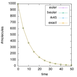
(b)

(c)

Figure 1: Average species count for birth-death process ($\mbox{ATOL}=$ (a) $10^{-10}$, (b) $10^{-12}$, (c) $10^{-14}$).

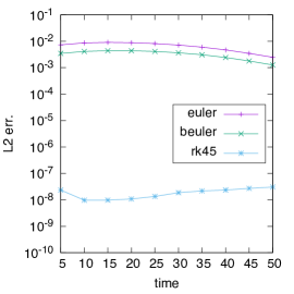
(a)

(b)

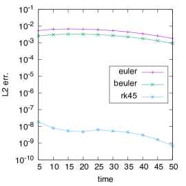
(c)

Figure 2: L2 error for birth-death model ($\mbox{ATOL}=$ (a) $10^{-10}$, (b) $10^{-12}$, (c) $10^{-14}$).

Figure 2 depicts plots of the L2 error

$$||p_{x}(t_{\eta})-p_{x}^{(\eta)}||_{2}$$

with $t_{\eta}=T=50$. The norm is computed over all states with positive probabilities in the exact solution. Note that if there is no corresponding state in $\mathit{Sig}$, its probability is taken as 0.

It can be seen that in all cases the L2 error is less than $10^{-2}$, which confirms the high accuracy of the approximations also formally. It can be further seen that for this example euler is slightly more accurate than beuler and that rk45 is even by orders of magnitude more accurate than the Euler schemes. This is well in accordance with the higher order of rk45.

Figure 3 shows the average step sizes taken by the different integration schemes, where rk45 takes much larger steps than the Euler schemes.

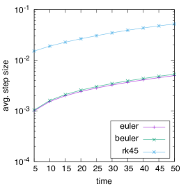
(a)

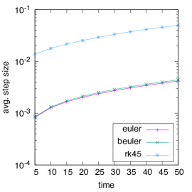
(b)

(c)

Figure 3: Average step sizes for birth-death process ($\mbox{ATOL}=$ (a) $10^{-10}$, (b) $10^{-12}$, (c) $10^{-14}$).

In Figure 4 we plot the numbers of significant states used during the computation. It can be seen that for all considered values of ATOL all integration schemes only require to handle (integrate) a moderate number of states (differential equations) where the Euler schemes require roughly the same number of states and rk45 requires only slightly more, in any case for any time less than $250$ states. Of course, the smaller ATOL (and thus our truncation probability threshold $\delta=\mbox{ATOL}$) the larger the number of significant states but with only a slight increase. This shows that the dynamical truncation procedure indeed substantially reduces the size of the state space and thus renders possible to integrate numerically with – as demonstrated by the previous figures – maintaining a high accuracy of the approximations.

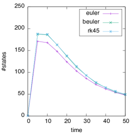
(a)

(b)

(c)

Figure 4: Numbers of significant states for birth-death process ($\mbox{ATOL}=$ (a) $10^{-10}$, (b) $10^{-12}$, (c) $10^{-14}$).

4.2 Yeast cell polarization

As another reference example we consider a stochastic model of the pheromone-induced G-protein cycle in the yeast Saccharomyces cerevisiae [11, 41, 45]

$$\emptyset \stackrel{{\scriptstyle c_{1}}}{{\longrightarrow}}\ R\quad c_{1}=0.0038\qquad RL+G \stackrel{{\scriptstyle c_{5}}}{{\longrightarrow}}G_{a}+G_{bg}\quad c_{5}=0.011$$

$$R \stackrel{{\scriptstyle c_{2}}}{{\longrightarrow}}\emptyset\quad c_{2}=0.0004\qquad G_{a} \stackrel{{\scriptstyle c_{6}}}{{\longrightarrow}}G_{d}\quad c_{6}=0.1$$

$$L+R \stackrel{{\scriptstyle c_{3}}}{{\longrightarrow}}RL+L\quad c_{3}=0.042\qquad G_{d}+G_{bg} \stackrel{{\scriptstyle c_{7}}}{{\longrightarrow}}G\quad c_{7}=1050.0$$

$$RL \stackrel{{\scriptstyle c_{4}}}{{\longrightarrow}}R\quad c_{4}=0.01\qquad \emptyset \stackrel{{\scriptstyle c_{8}}}{{\longrightarrow}}RL\quad c_{8}=3.21$$

with initial state $x(0)=(50,2,0,50,0,0,0)$, where the state vector is given as $x=(R,L,RL,G,G_{a},G_{bg},G_{d})$ and the state space is the infinite $7$-dimensional set ${\mathbb{N}}^{7}$. Note that in order to keep the meaning of the species here we do not number the species but take the notation from [45].

In Figure 5 we plot the average species counts computed using rk45 with $\mbox{ATOL}=10^{-15}$ and the numbers of significant states for rk45 over time for different values of $\mbox{ATOL}\in\{10^{-10},10^{-12},10^{-14},10^{-15}\}$.

(a)

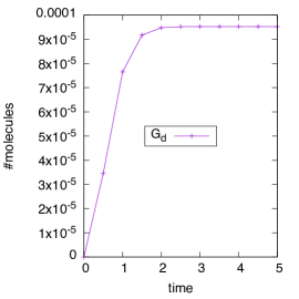
(b)

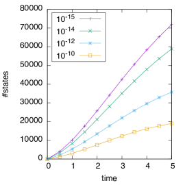
(c)

Figure 5: Yeast cell polarization: (a,b) average species counts, (c) number of significant states for different values of ATOL.

Note that as in the previous example the numbers of significant states as well as the average numbers of species for euler and beuler only slightly differ from those for rk45, so that we omit to include them in the plots. It is clear that in the much more complex yeast cell polarization model there are many more significant states than in the birth-death process, but the numbers of significant states are still in a range that allows accurate approximations in reasonable time.

In Table 1 we list the run times for different values of ATOL. We can see that in this example beuler heavily outperforms the explicit methods euler and rk45. This confirms the advantages of implicit methods over explicit methods for stiff systems. In fact, while the birth-death example is not or only moderately stiff, the yeast cell polarization model constitutes a very stiff system of differential equations.

Table 1: Run times for yeast cell polarization model.

method	$\mbox{ATOL}=10^{-10}$	$\mbox{ATOL}=10^{-12}$	$\mbox{ATOL}=10^{-14}$
euler	761s	1481s	5839s
beuler	35s	76s	139s
rk45	5806s	18603s	26126s

In Figure 6 we plot the average step size over time and the L2 error for $\mbox{ATOL}=10^{-14}$. Since there is no analytical solution, we compute the L2 with respect to the distribution obtained using rk45 with a lower absolute tolerance $\mbox{ATOL}=10^{-15}$, applying the rationale that with an even lower error tolerance the method gives nearly exact values. The respective L2 errors for $\mbox{ATOL}=10^{-10}$ and $\mbox{ATOL}=10^{-12}$ are similar.

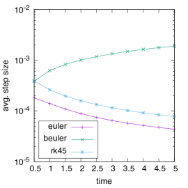
(a)

(b)

Figure 6: (a) Average step sizes and (b) L2 error for yeast polarization model ($\mbox{ATOL}=10^{-14}$).

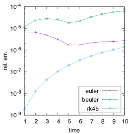
(a)

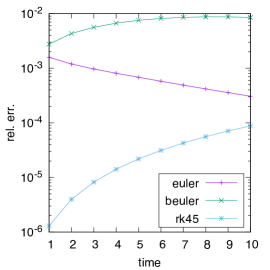
(b)

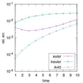
(c)

Figure 7: Relative errors.

5 Conclusion

We have shown that our numerical integration approach with adaptive step size selection based on local error estimates performed in combination with dynamical state space truncation provides a versatile means of approximating the solution of the chemical master equation for complex stochastic reaction networks efficiently and accurately. The state space explosion problem is circumvented by considering in each time step only such states of the overall state space of the reaction network that have at that time step a significant (sufficiently large according to a flexibly adjustable bound) probability, that is, in the course of the integration scheme we keep the number of differential equations to be integrated per step manageable. By a framework that includes explicit as well as implicit integration schemes we offer the flexibility to choose an appropriate integration scheme that is well-suited with regard to the specific dynamics of a given reaction network.

In order to provide meaningful, detailed comparisons of different methods with different parameter choices and to study their impact on accuracy, run times and numbers of significant states to be processed we have considered the explicit Euler method, an explicit Runge-Kutta as an extension of explicit Euler, and the implicit (backward) Euler method, all equipped with a well-suited adaptive step size selection strategy and performed on the dynamically truncated state space. The results show that the proposed approximate numerical integration of the chemical master equation indeed yields satisfactorily accurate results in reasonable time. Future research will be concerned with further advanced integration schemes, to equip them similarly with adaptive step size selection strategies and to study the accuracy and the run times. Of course, also in-depth theoretical investigations of the performance, efficiency and accuracy of the approximate numerical integration approach are highly desirable.

References

- [1] D. F. Anderson. Incorporating postleap checks in tau-leaping. Journal of Chemical Physics, 128(5):054103, 2008.
- [2] A. Andreychenko, W. Sandmann, and V. Wolf. Approximate adative uniformization of continuous-time Markov chains. Applied Mathematical Modelling, 61:561–576, 2018.
- [3] A. B. Bortz, M. H. Kalos, and J. L. Lebowitz. A new algorithm for Monte Carlo simulation of Ising spin systems. Journal of Computational Physics, 17:10–18, 1975.
- [4] K. Burrage, M. Hegland, S. MacNamara, and R. Sidje. A Krylov-based finite state projection algorithm for solving the chemical master equation arising in the discrete modelling of biological systems. In A. N. Langville and W. J. Stewart, editors, Proceedings of the Markov Anniversary Meeting: An International Conference to Celebrate the 150th Anniversary of the Birth of A. A. Markov, pages 21–38, 2006.
- [5] K. Burrage, T. Tian, and P. Burrage. A multi-scaled approach for simulating chemical reaction systems. Progress in Biophysics and Molecular Biology, 85:217–234, 2004.
- [6] H. Busch, W. Sandmann, and V. Wolf. A numerical aggregation algorithm for the enzyme-catalyzed substrate conversion. In Proceedings of the 2006 International Conference on Computational Methods in Systems Biology, volume 4210 of Lecture Notes in Computer Science, pages 298–311. Springer, 2006.
- [7] J. C. Butcher. Numerical Methods for Ordinary Differential Equations. John Wiley & Sons, 2nd edition, 2008.
- [8] Y. Cao, D. T. Gillespie, and L. R. Petzold. Efficient stepsize selection for the tau-leaping simulation. Journal of Chemical Physics, 124:044109–144109–11, 2006.
- [9] Y. Cao, D. T. Gillespie, and L. R. Petzold. The adaptive explicit-implicit tau-leaping method with automatic tau selection. Journal of Chemical Physics, 126(22):224101, 2007.
- [10] Y. Cao, H. Li, and L. R. Petzold. Efficient formulation of the stochastic simulation algorithm for chemically reacting systems. Journal of Chemical Physics, 121(9):4059–4067, 2004.
- [11] C.-S. Chou, Q. Nie, and T.-M. Yi. Modeling robustness tradeoffs in yeast cell polarization induced by spatial gradients. PLoS ONE, 3(9):e3103, 2008.
- [12] E. de Souza e Silva and P. M. Ochoa. State space exploration in Markov models. In Proceedings of the ACM SIGMETRICS Joint International Conference on Measurement and Modeling of Computer Systems, pages 152–166, 1992.
- [13] J. R. Dormand and P. J. Prince. A family of embedded Runge-Kutta formulae. Journal of Computational and Applied Mathematics, 6(1):19–26, 1980.
- [14] W. E., D. Liu, and E. Vanden-Eijnden. Nested stochastic simulation algorithms for chemical kinetic systems with multiple time scales. Journal of Computational Physics, 221:158–180, 2007.
- [15] M. A. Gibson and J. Bruck. Efficient exact stochastic simulation of chemical systems with many species and many channels. Journal of Physical Chemistry, A 104:1876–1889, 2000.
- [16] D. T. Gillespie. A general method for numerically simulating the time evolution of coupled chemical reactions. Journal of Computational Physics, 22:403–434, 1976.
- [17] D. T. Gillespie. Exact stochastic simulation of coupled chemical reactions. Journal of Physical Chemistry, 71(25):2340–2361, 1977.
- [18] D. T. Gillespie. A rigorous derivation of the chemical master equation. Physica A, 188:404–425, 1992.
- [19] D. T. Gillespie. Approximate accelerated stochastic simulation of chemically reacting systems. Journal of Chemical Physics, 115:1716–1732, 2001.
- [20] E. Hairer, S. P. Nørsett, and G. Wanner. Solving Ordinary Differential Equations I: Nonstiff Problems. Springer-Verlag, Berlin Heidelberg, 2nd edition, 1993.
- [21] E. Hairer and G. Wanner. Solving Ordinary Differential Equations II: Stiff and Differential-Algebraic Problems. Springer-Verlag, Berlin Heidelberg, 2nd edition, 1996.
- [22] L. A. Harris and P. Clancy. A partitioned leaping approach for multiscale modeling of chemical reaction dynamics. Journal of Chemical Physics, 125(14):144107, 2006.
- [23] E. L. Haseltine and J. B. Rawlings. Approximate simulation of coupled fast and slow reactions for stochastic chemical kinetics. Journal of Chemical Physics, 117(15):6959–6969, 2002.
- [24] A. Hellander and P. Lötstedt. Hybrid method for the chemical master equation. Journal of Computational Physics, 227:100–122, 2007.
- [25] T. Jahnke. An adaptive wavelet method for the chemical master equation. SIAM Journal on Scientific Computing, 31(6):4373 –4394, 2010.
- [26] T. Jahnke and W. Huisinga. Solving the chemical master equation for monomolecular reactions analytically. Journal of Mathematical Biology, 54(1):1–26, 2007.
- [27] T. Jahnke and T. Udrescu. Solving chemical master equations by adaptive wavelet compression. Journal of Computational Physics, 229:5724–5741, 2010.
- [28] T. G. Kurtz. The relationship between stochastic and deterministic models for chemical reactions. Journal of Chemical Physics, 57(7):2976–2978, 1972.
- [29] I. J. Laurenzi. An analytical solution of the stochastic master equation for reversible bimolecular reaction kinetics. Journal of Chemical Physics, 113(8):3315–3322, 2000.
- [30] H. Li and L. R. Petzold. Logarithmic direct method for discrete stochastic simulation of chemically reacting systems. Technical Report, Department of Computer Science, University of California, Santa Barbara, 2006. http://www.engineering.ucsb.edu/cse/Files/ldm0513.pdf.
- [31] S. MacNamara, A. M. Bersani, K. Burrage, and R. B. Sidje. Stochastic chemical kinetics and the total quasi-steady-state assumption: application to the stochastic simulation algorithm and chemical master equation. Journal of Chemical Physics, 129:095105, 2008.
- [32] S. MacNamara, K. Burrage, and R. B. Sidje. Multiscale modeling of chemical kinetics via the master equation. Multiscale Modeling & Simulation, 6(4):1146–1168, 2008.
- [33] M. Mateescu, V. Wolf, F. Didier, and T.A. Henzinger. Fast adaptive uniformisation of the chemical master equation. IET Systems Biology, 4(6):441–452, 2010.
- [34] J. M. McCollum, G. D. Peterson, C. D. Cox, M. L. Simpson, and N. F. Samatova. The sorting direct method for stochastic simulation of biochemical systems with varying reaction execution behavior. Computational Biology and Chemistry, 30(1):39–49, 2006.
- [35] L. Mikeev, W. Sandmann, and V. Wolf. Efficient calculation of rare event probabilities in Markovian queueing networks. In Proceedings of the 5th International Conference on Performance Evaluation Methodologies and Tools, VALUETOOLS, pages 186–196, 2011.
- [36] L. Mikeev, W. Sandmann, and V. Wolf. Numerical approximation of rare event probabilities in biochemically reacting systems. In A. Gupta and T. A. Henzinger, editors, Proceedings of the 11th International Conference on Computational Methods in Systems Biology, CMSB, volume 8130 of Lecture Notes in Bioinformatics, pages 5–18. Springer, 2013.
- [37] C. Moler and C. Van Loan. Nineteen dubious ways to compute the exponential of a matrix. SIAM Review, 20:801–836, 1978.
- [38] C. Moler and C. Van Loan. Nineteen dubious ways to compute the exponential of a matrix, twenty-five years later. SIAM Review, 45:3–49, 2003.
- [39] B. Munsky and M. Khammash. The finite state projection algorithm for the solution of the chemical master equation. Journal of Chemical Physics, 124:044104, 2006.
- [40] B. Munsky and M. Khammash. A multiple time interval finite state projection algorithm for the solution to the chemical master equation. Journal of Computational Physics, 226:818–835, 2007.
- [41] D. Pruyne and A. Bretcher. Polarization of cell growth in yeast I. Establishment and maintenance of polarity states. Journal of Cell Science, 113:365–375, 2000.
- [42] C. V. Rao and A. Arkin. Stochastic chemical kinetics and the quasi-steady-state-assumption: Application to the Gillespie algorithm. Journal of Chemical Physics, 118:4999–5010, 2003.
- [43] M. Rathinam and H. El Samad. Reversible-equivalent-monomolecular tau: A leaping method for small number and stiff stochastic chemical systems. Journal of Computational Physics, 224:897–923, 2007.
- [44] M. Rathinam, L. R. Petzold, Y. Cao, and D. T. Gillespie. Stiffness in stochastic chemically reacting systems: The implicit tau-leaping method. Journal of Chemical Physics, 119:12784–12794, 2003.
- [45] M. K. Roh, B. J. Daigle Jr., D. T. Gillespie, and L. R. Petzold. State-dependent doubly weighted stochastic simulation algorithm for automatic characterization of stochastic biochemical rare events. Journal of Chemical Physics, 135:234108, 2011.
- [46] C. Safta, K. Sargsyan, B. Debusschere, and H. N. Najm. Hybrid discrete/continuum algorithms for stochastic reaction networks. Journal of Computational Physics, 281:177–198, 2015.
- [47] H. Salis and Y. Kaznessis. Accurate hybrid stochastic simulation of a system of coupled chemical or biochemical reactions. Journal of Chemical Physics, 122:054103, 2005.
- [48] W. Sandmann. Discrete-time stochastic modeling and simulation of biochemical networks. Computational Biology and Chemistry, 32(4):292–297, 2008.
- [49] W. Sandmann. Sequential estimation for prescribed statistical accuracy in stochastic simulation of biological systems. Mathematical Biosciences, 221(1):43–53, 2009.
- [50] W. Sandmann. Streamlined formulation of adaptive explicit-implicit tau-leaping with automatic tau selection. In Proceedings of the 2009 Winter Simulation Conference, pages 1104–1112, 2009.
- [51] W. Sandmann and V. Wolf. Computational probability for systems biology. In Proceedings of the Workshop on Formal Methods in Systems Biology, volume 5054 of Lecture Notes in Computer Science, pages 33–47. Springer, 2008.
- [52] L. F. Shampine, I. Gladwell, and S. Thompson. Solving ODEs with MATLAB. Cambridge University Press, 2003.
- [53] T. Tian and K. Burrage. Binomial leap methods for simulating stochastic chemical kinetics. Journal of Chemical Physics, 121:10356–10364, 2004.
- [54] N. van Kampen. Stochastic Processes in Physics and Chemistry. Elsevier, North-Holland, 1992.
- [55] K. Vasudeva and U. S. Bhalla. Adaptive stochastic-deterministic chemical kinetics simulation. Bioinformatics, 20(1):78–84, 2004.
- [56] Z. Xu and W. Cai. Unbiased tau-leaping methods for stochastic simulation of chemically reacting systems. Journal of Chemical Physics, 128(15):154112, 2008.