Mixed-Supervised Dual-Network for Medical Image Segmentation

Abstract

Deep learning based medical image segmentation models usually require large datasets with high-quality dense segmentations to train, which are very time-consuming and expensive to prepare. One way to tackle this challenge is using the mixed-supervised learning framework, in which only a part of data is densely annotated with segmentation label and the rest is weakly labeled with bounding boxes. The model is trained jointly in a multi-task learning setting. In this paper, we propose Mixed-Supervised Dual-Network (MSDN), a novel architecture which consists of two separate networks for the detection and segmentation tasks respectively, and a series of connection modules between the layers of the two networks. These connection modules are used to transfer useful information from the auxiliary detection task to help the segmentation task. We propose to use a recent technique called Squeeze and Excitation in the connection module to boost the transfer. We conduct experiments on two medical image segmentation datasets. The proposed MSDN model outperforms multiple baselines.

1 Introduction

Image segmentation is an important application of medical image analysis. Recently, deep learning based methods [1, 2, 3, 4] have achieved remarkable success in many medical image segmentation tasks, such as brain tumor and lung nodule segmentation. However, all these methods require a large amount of training data with high-quality dense annotations to train, which is very expensive and time-consuming to prepare.

Therefore, weakly-supervised segmentation with insufficient labels, e.g. image tags [5] or bounding boxes [6] has attracted a lot of attention recently. Although great progress has been made, there still exists some gap in performance compared to the models trained with fully-supervised datasets. This makes it impractical for the medical image scenario, where accurate segmentation maps are required for disease diagnosis, surgical planning or pathological analysis. On the other hand, these weakly-supervised models are usually trained in multi-step iteration mode [5, 6] or with prior medical knowledge [7], making it difficult to be scalable on real applications.

Another promising approach is the mixed-supervised segmentation, where only a part of data is densely annotated with segmentation map and the rest is labeled with weak form (such as with bounding boxes). Typical existing methods [8, 14, 15] consider training with such kind of data in a multi-task learning setting and exploit multi-stream network, where basic feature extractor is shared and different streams are used for data with different annotation forms. The work in [15] focuses on the optimal balance between the number of annotations needed for different supervision types and presents a budget-based cost-minimization framework in a mixed-supervision setting.

In this paper, we propose a novel architecture for mixed-supervised medical image segmentation. Considering the bounding boxes as weak annotation, our method takes the segmentation task as target task, which is augmented with object detection task (auxiliary task). Different from the multi-stream structure with shared backbone [8], our new architecture is made up of two separate networks for each task. The two networks are linked by a series of connection modules that lie between the corresponding layers. These connection modules take as input the convolution features of detection network and transfer useful information to the segmentation network to help the training of the segmentation task. We propose to use a recent feature attention technique called “Squeeze and Excitation” [9, 10, 13] in the connection module to boost the information transfer. The proposed model is named as Mixed-Supervised Dual-Network (MSDN). We perform evaluation on the lung nodule segmentation and the cochlea segmentation of CT images. Experimental results show that our model is able to outperform multiple baseline approach in both datasets.

2 Methods

2.1 Squeeze and Excitation

“Squeeze-and-Excitation” (SE) was first introduced in [9] and can be flexibly integrated in any CNN model. The SE module first squeezes the feature map by global average pooling and then passes the squeezed feature to the gating module to get the representation of channel-wise dependencies, which is used to re-calibrate the feature map to emphasize on useful channels. The work in [10] refers to the SE module in [9] as Spatial Squeeze and Channel Excitation (cSE) and proposes a different version called Channel Squeeze and Spatial Excitation (sSE). The sSE module squeezes the feature map along channels to preserve more spatial information, thus is more suitable for image segmentation task. The two SE modules mentioned above are unary, as both the squeeze and excitation are operated on the same feature map. Abhijit et al. [13] builds a binary version of sSE and applies it to their two-armed architecture for few-shot segmentation. Since the sSE module is related to our method, we will give a more detailed introduction as follows (see Fig. 1).

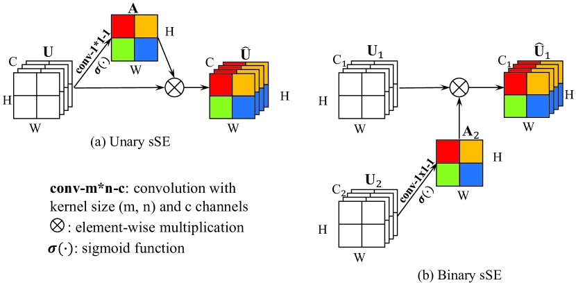
Figure 1: Illustration of the Channel Squeeze and Spatial Excitation (sSE) architecture of Unary form (a) and Binary form (b).

We consider the feature map U = [$\textbf{{u}}^{1}$, $\textbf{{u}}^{2}$, …, $\textbf{{u}}^{C}$] from previous convolution layer as the input of the Unary sSE module and $u^{i}$ $\in$ $\mathbb{R}^{W\times H}$ denotes its $i$th channel. The channel squeeze operation is achieved by 1 $\times$ 1 convolution with kernel weight $\textbf{{w}}_{sq}$ $\in$ $\mathbb{R}^{1\times C\times 1\times 1}$. The squeezed feature is then passed through sigmoid function to derive the attention weight A $\in$ $\mathbb{R}^{W\times H}$. Then each feature channel of U is multiplied element-wise by A to get the spatially recalibrated feature $\widehat{\textbf{{U}}}$ as output

$$\widehat{\mathbf{U}}=[\sigma(\mathbf{w}_{sq}*\mathbf{U})\circ\mathbf{u}^{1},\sigma(\mathbf{w}_{sq}*\mathbf{U})\circ\mathbf{u}^{2},...,\sigma(\mathbf{w}_{sq}*\mathbf{U})\circ\mathbf{u}^{C}]$$ (1)

Here $\circ$ denotes the Hadamard product, * denotes the convolution operation and $\sigma$ denotes the sigmoid function.

Binary sSE extends the idea of Unary sSE, which takes two feature maps as inputs. One feature map is squeezed and used to recalibrate the other feature as output

$$\widehat{\mathbf{U}}_{1}=[\sigma(\mathbf{w}_{sq}*\mathbf{U}_{2})\circ\mathbf{u}^{1}_{1},\sigma(\mathbf{w}_{sq}*\mathbf{U}_{2})\circ\mathbf{u}^{2}_{1},...,\sigma(\mathbf{w}_{sq}*\mathbf{U}_{2})\circ\mathbf{u}^{C}_{1}]$$ (2)

We propose to use the Binary sSE module as the connection between our dual-network architecture for information extraction and transfer.

2.2 Architectural Design

Our MSDN follows the setting of multi-task learning and is made up of two separate sub-networks for the segmentation and detection tasks respectively (as shown in Fig. 2). Both sub-networks are built from the U-Net and contain 9 feature stages, with 4 stages in the Encoder, 4 in the Decoder and 1 in the Bottleneck. Each feature stage consists of 2 dilated-convolution layers with 3*3 kernel, each followed by batch normalization [12] and rectified linear unit(ReLU). The output of each Encoder stage is skip-connected to the corresponding Decoder stage to recover spatial information lost during max-pooling [20]. Dilation factors are set as [1,2,2,2,4,2,2,2,1] in the 9 feature stages respectively. The stride and padding are chosen accordingly to make the size of the output feature identical to that of the input.

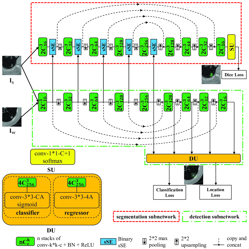
Figure 2: Structure of Mixed-Supervised Dual-Network (MSDN).

For the segmentation sub-network, the sSE modules are added after each stage in its Encoder and Bottleneck, which take the segmentation and detection features from the same stage as input, squeeze the detection feature and re-calibrate the segmentation feature. In this way, the segmentation sub-network can extract useful information from the auxiliary detection sub-network to facilitate its training.

The Segmentation Unit (SU) takes the extracted features into a 1*1 convolution layer followed by a channel-wise soft-max to output a dense segmentation map with C+1 channels, where C is the number of segmentation classes and we treat the background as another class. Dice loss [2] is used for the segmentation sub-network training.

For the detection sub-network, we build the Detection Unit (DU) under a single-stage object-detection paradigm, similarly to [8, 11]. The DU consists of a classifier block and a bounding box regressor block and takes as input the convolution feature from the detection sub-network and produces class predictions for C target classes and object locations via bounding boxes. Note that all features from the Decoder stages are used for detection and the parameters of DU are shared. At each position of the feature, totally A=9 reference bounding boxes of different shapes and sizes are built as anchors. The DU predicts the class label (C-length vector) of the object and the relative position (4-length vector) to the near ground-truth bounding boxes for each of the A anchors. Thus, the classifier(regressor) takes the feature from the Decoder of the detection sub-network through 4 3*3 convolution layers with 256 channels and one 3*3 convolution layer with C*A(4*A) channels. A Sigmoid function is used to scale the output of classifier to [0, 1]. The detection loss is the sum of the cross-entropy based focal loss for classification and the regularized-L1 loss for location [11].

During training, we mix the strongly- and weakly-annotated data and shuffle them. At each training iteration, we randomly select a batch of data as the input to our model. The strongly-annotated data $\textbf{{I}}_{\textrm{s}}$ goes through the Encoder of the detection and segmentation sub-networks and its segmentation features are re-calibrated by the detection features for the Decoder to derive the segmentation loss. The weakly-annotated data $\textbf{{I}}_{\textrm{w}}$ only goes through the detection sub-network to get the detection loss. The sum of the segmentation loss and detection loss is minimized to train the model.

The structure of our model is similar to that in [13], as we both build a dual architecture with two sub-networks and exploit sSE modules as connection. However, the work [13] focuses on the few-shot segmentation problem. The two sub-networks are used for the same segmentation task and trained jointly in the meta-learning mode. sSE modules exist in every feature stage of the base network. While, our model is designed for mixed-supervised segmentation problem, the two networks are used for different tasks and trained iteratively in multi-task learning mode. Because of that, the features of the two sub-networks in shallow layers may be relative to each other and those in deep layers may be task-specific. So we only use sSE in the shallow layers, specifically, in the Encoder and Bottleneck.

3 Experiments

We evaluate our model on two medical image segmentation datasets: lung nodule dataset and cochlea of inner ear dataset. The lung dataset consists of non-contrast CT of 320 nodules that was acquired on a 64-detector CT system (GE Light Speed VCT or GE Discovery CT750 HD, GE Healthcare, Milwaukee, WI, USA) using the scan parameters: section width, 1.25 mm; reconstruction interval, 1.25 mm; pitch, 0.984; 120 kV; and 35 mA; display field of view (DFOV) ranged from 28cm to 36 cm; matrix size, 512*512, pixel size ranged from 0.55mm to 0.7mm. We randomly choose 160, 80 and 80 as training, validating and testing dataset. The inner ear dataset consisted of non-contrast temporal bone CT of 146 cochleas that was acquired on a Siemens Somatom scanner using the scan parameters: 120 kV; 167 mA, slice thickness, 1mm; matrix size, 512*512, and pixel size, 0.40625. 66, 40 and 40 images are randomly split as training, validating and testing dataset. 5 different proportions of strongly-annotated data are tested. For both datasets, we measure the performance by the Dice score of target segmentation structure between the estimated and true label maps.

We use the Adam optimizer [17] to train all the models. The initial learning rate is set to 0.0001 and is reduced by a factor of 0.8 if the mean validation Dice score doesn’t increase in 5 epochs. The training is stopped if the score doesn’t increase by 20 epochs. Dropout [16] is used to the output of each convolution stage to avoid over-fitting. During the training, we use a mini-batch of 4 images and if the validation Dice score goes up, we evaluate the model on the testing dataset. The best testing Dice score is reported as the final result. We perform data augmentation through random horizontal and vertical flipping, adding Gaussian noise and randomly cropping the image to a 128*128 patch centered around the target structure. All images are normalized by subtracting the mean and dividing by the standard deviation of the training data.

Table 1: Mean of test Dice score (%).

Lung Nodule Segmentation
Methods	strong-weak data split(160 in total)
	160-0	120-40	100-60	80-80	60-100
U-Net	84.04$\pm$0.40	82.25$\pm$0.39	81.85$\pm$0.31	80.51$\pm$0.59	80.18$\pm$0.97
U-Net+Unary sSE	84.01$\pm$0.11	82.15$\pm$1.09	81.35$\pm$1.39	82.08$\pm$0.94	80.58$\pm$0.01
Variant MS-Net[8]	-	82.75$\pm$1.04	82.38$\pm$0.53	81.72$\pm$1.19	79.80$\pm$1.26
MSDN-	84.90$\pm$0.60	82.31$\pm$1.14	82.17$\pm$0.51	81.02$\pm$1.10	80.50$\pm$0.37
MSDN	-	83.58$\pm$1.20	83.56$\pm$0.52	83.01$\pm$0.69	82.37$\pm$0.98
Cochlea Segmentation
Methods	strong-weak data split(66 in total)
	66-0	44-22	33-33	22-44	11-55
U-Net	88.62$\pm$0.08	87.41$\pm$0.16	86.55$\pm$0.81	85.01$\pm$0.39	80.85$\pm$0.42
U-Net+Unary sSE	88.97$\pm$0.12	87.70$\pm$0.49	85.30$\pm$0.28	84.38$\pm$0.03	82.23$\pm$0.47
Variant MS-Net[8]	-	87.54$\pm$0.36	86.03$\pm$0.25	84.71$\pm$0.53	82.60$\pm$1.43
MSDN-	88.73$\pm$0.33	86.73$\pm$1.02	85.68$\pm$0.35	85.10$\pm$0.15	80.81$\pm$0.47
MSDN	-	87.91$\pm$0.28	87.27$\pm$1.08	87.11$\pm$0.28	85.60$\pm$1.76

We compare MSDN with other 4 baselines, as shown in Table. 1. All the models are trained following the same setting described aforementioned. A U-Net with the same number of convolution layers as the segmentation sub-network of our model is used. For the U-Net+Unary sSE, Unary sSE module is added after every convolution stage. For the Variant MS-Net, we follow the thought of MS-Net [8] and build a multi-stream network based on U-Net, where all features from the Decoder are taken into the detection stream DU. We also compare to a reduced version of our model (MSDN-), where we remove the DU and only preserve the U-NET and the Binary sSE modules. Note that the U-Net, U-Net+Unary sSE and MSDN- are trained only with strongly-annotated data. We run each experiment repeatly for 3 times and the mean dice score with 95% confidence interval is listed in Table. 1.

From the result, we can see that our model performs better than all the baselines in the same strong-weak data split. Compared with models trained in a fully-supervised manner, the performance is still comparable. When there are few strongly-annotated data for training, the performances of baselines decrease dramatically (see the last column). However, the performance of our model still remains good. The variation of MS-Net improves the results in some degree, but sometimes the performance is not stable. In contrast, our model works more stably. The use of sSE module, no matter Unary or Binary, could improve the training effect, but not as much as our model, which proves the effectiveness of our design. Some qualitative results are shown in Fig. 3.

4 Conclusion and Future Work

We propose Mixed-Supervised Dual-Network (MSDN), a novel multi-task learning architecture for mixed-supervised medical image segmentation. It is composed of two separate networks for the detection and segmentation tasks respectively, and a series of sSE modules as connection between the two networks so that the useful information of the detection task can be transferred to facilitate the segmentation task well. We perform experiments on two medical image datasets and our model outperforms multiple baselines. Currently, our model can only handle two-task problem. When there are more than two forms of annotations, our model can not directly be applied. In the future, we may consider to extend our method to fit for multi-task scenario [18, 19].

4.0.1 Acknowledgement

This research is supported by China Scholarship Council (CSC).

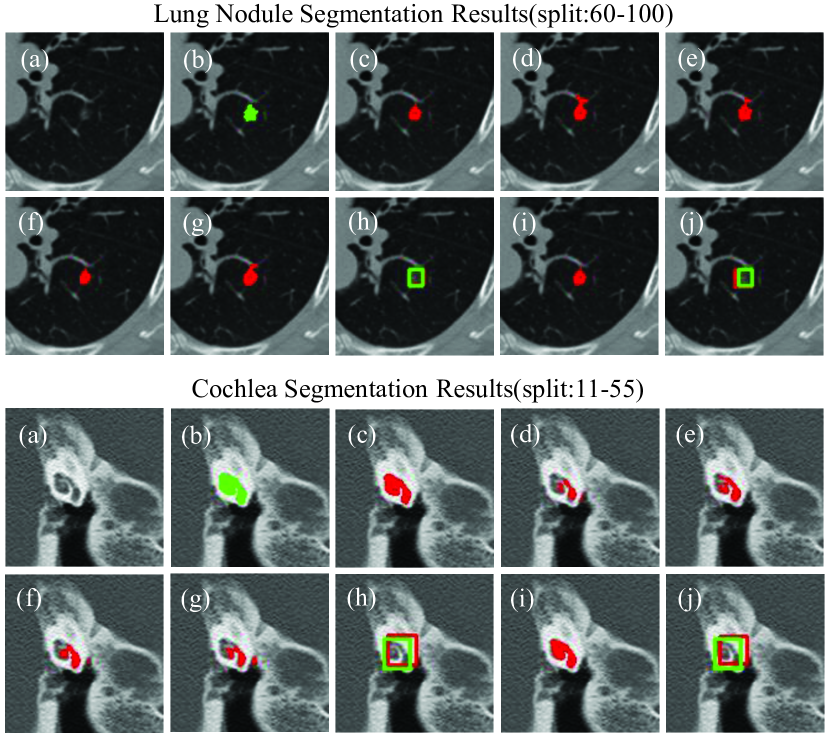
Figure 3: (a) Original image. (b) Ground truth. (c) U-Net trained in full-supervised manner. (d) U-Net trained with only strongly-annotated data. (e) U-Net+Unary sSE. (f) MSDN-. (g),(h) Segmentation and detection results of Variant MS-Net. (i),(j) Segmentation and detection results of MSDN.

References

- [1] Ronneberger, O., Fischer, P., Brox, T.: U-net: Convolutional networks for biomedical image segmentation. In MICCAI 2015. LNCS, vol. 9351, pp. 234 241 (2015).
- [2] Milletari, F., Navab, N., Ahmadi, S.: V-net: Fully convolutional neural networks for volumetric medical image segmentation. In: International Conference on 3D Vision, pp. 565 571 (2016)
- [3] Jiang, J., Hu, YC., Liu, CJ., et al: Multiple Resolution Residually Connected Feature Streams for Automatic Lung Tumor Segmentation From CT Images. IEEE Trans. Med. Imaging 38(1): 134-144 (2019).
- [4] Fan, G., Liu, H., Wu,Z., et al: Deep Learning Based Automatic Segmentation of Lumbosacral Nerves on CT for Spinal Intervention: A Translational Study. American Journal of Neuroradiology 40(6): 1074-1081 (2019).
- [5] Wang, X., You, S., Li, X., Ma, H.: Weakly-supervised semantic segmentation by iteratively mining common object features. In CVPR 2018, pp. 1354-1362 (2018)
- [6] Rajchl, M., Lee, M. C., Oktay, O., et al: Deepcut: Object segmentation from bounding box annotations using convolutional neural networks. IEEE Trans. Med. Imaging, 36(2), 674-683 (2017).
- [7] Kervadec, H., Dolz, J., Tang, M., et al: Constrained-CNN losses for weakly supervised segmentation. Medical image analysis 54, 88-99 (2019).
- [8] Shah, M.P., Merchant, S.N., Awate, S.P.: MS-Net: Mixed-Supervision Fully-Convolutional Networks for Full-Resolution Segmentation. In MICCAI 2018. LNCS, vol 11073, pp. 379-387(2018).
- [9] Hu, J., Shen, L., Sun, G.: Squeeze-and-excitation networks. In CVPR 2018, pp. 7132-7141 (2018).
- [10] Roy, A.G., Navab, N., Wachinger, C.: Concurrent Spatial and Channel Squeeze and Excitation in Fully Convolutional Networks. In MICCAI 2018. LNCS, vol 11070, pp. 421-429 (2018).
- [11] Lin, T.Y., Goyal, P., Girshick, R., He, K., Doll r, P.: Focal loss for dense object detection. In ICCV 2017, pp. 2980-2988 (2017).
- [12] Ioffe, S., Szegedy, C.: Batch normalization: Accelerating deep network training by reducing internal covariate shift. In ICML 2015, pp. 448-456 (2015).
- [13] Roy, A.G., Siddiqui, S., P lsterl, S., et al: Squeeze and Excite’ Guided Few-Shot Segmentation of Volumetric Images. arXiv preprint arXiv:1902.01314 (2019).
- [14] Mlynarski, P., Delingette, H., Criminisi, A., et al: Deep Learning with Mixed Supervision for Brain Tumor Segmentation. arXiv preprint arXiv:1812.04571 (2018).
- [15] Bhalgat, Y., Shah, M., Awate, S.: Annotation-cost Minimization for Medical Image Segmentation using Suggestive Mixed Supervision Fully Convolutional Networks. arXiv preprint arXiv:1812.11302 (2018).
- [16] Srivastava, N., Hinton, G., Krizhevsky, A., et al: Dropout: a simple way to prevent neural networks from overfitting. J. Mach. Learn. Res. 15(1), 1929 1958 (2014)
- [17] Kingma, D.P., Ba, J.: Adam: A method for stochastic optimization. arXiv preprint arXiv:1412.6980 (2014).
- [18] Y. Lu, A. Kumar, S. Zhai, Y. Cheng, T. Javidi, and R. S. Feris. Fully-adaptive feature sharing in multi-task networks with applications in person attribute classification. CVPR, 2017.
- [19] J. Wang, Y. Cheng, and R. Schmidt Feris. Walk and learn: Facial attribute representation learning from egocentric video and contextual data. CVPR, 2016.
- [20] S. Zhai, H. Wu, A. Kumar, Y. Cheng, Y. Lu, Z. Zhang, and R. S. Feris, S3pool: Pooling with stochastic spatial sampling. CVPR, 2017.