UNIQUE DIAGRAM OF A SPATIAL ARC AND THE KNOTTING PROBABILITY

ABSTRACT

It is shown that the projection image of an oriented spatial arc to any oriented plane is approximated by a unique arc diagram (up to isomorphic arc diagrams) determined from the spatial arc and the projection. In a separated paper, the knotting probability of an arc diagram is defined as an invariant under isomorphic arc diagrams. By combining them, the knotting probability of every oriented spatial arc is defined.

x

Keywords: Arc diagram,  Approximation, Spatial arc,  Knotting probability.

Mathematics Subject Classification 2010: Primary 57M25; Secondary 57Q45

1. Introduction

A spatial arc is a polygonal arc in the 3-space ${\mathbf{R}}^{3}$, which is considered as a model of a protein or a linear polymer in science. The following question on science is an interesting question that can be set as a mathematical question:

x

Question. How a linear scientific object such as a linear molecule (e.g. a non-circular DNA, protein, linear polymer,…) is considered as a knot object ?

x

In this paper, it is shown that the projection image of an oriented spatial arc to any oriented plane is approximated into a unique arc diagrams (up to isomorphic arc diagrams) determined from the spatial arc and the projection. Further, the orientation change of the spatial arc makes only substitutes for these unique arc diagrams (up to isomorphic arc diagrams). This argument is more or less similar to an argument transforming a classical knot in ${\mathbf{R}}^{3}$ into a regular knot diagram (see [1], [2]). Let

$$S^{2}=\{u\in{\mathbf{R}}^{3}|\,||u||=1\}$$

be the unit sphere, where $||\phantom{u}||$ denotes the norm on ${\mathbf{R}}^{3}$. Every element $u\in S^{2}$ is regarded as a unit vector from the origin $0$. For a unit vector $u\in{\mathbf{R}}^{3}$, let $P_{u}$ be the oriented plane containing the origin $0$ such that the unit vector $u$ is a positively normal vector to $P_{u}$. The orthogonal projection from ${\mathbf{R}}^{3}$ to the plane $P_{u}$ is called the projection along the unit vector $u\in S^{2}$ and denoted by

$$\lambda_{u}:{\mathbf{R}}^{3}\to P_{u}.$$

For a small positive number $\delta$, a $\delta$-approximation of the projection $\lambda_{u}:{\mathbf{R}}^{3}\to P_{u}$ along $u\in S^{2}$ is the projection

$$\lambda_{u^{\prime}}:{\mathbf{R}}^{3}\to P_{u^{\prime}}$$

along a unit vector $u^{\prime}\in S^{2}$ with $||u^{\prime}-u||<\delta$, which is denoted by

$$\lambda_{u}^{\delta}:{\mathbf{R}}^{3}\to P_{u}.$$

The projection image $\lambda_{u}(L)$ of a spatial arc $L$ in the plane $P_{u}$ is an arc diagram in the oriented plane $P_{u}$ if $\lambda_{u}(L)$ has only crossing points (i.e., transversely meeting double points with over-under information) and the starting and terminal points as single points. The arc diagram $(P_{u},\lambda_{u}(L))$ is sometimes denoted by $(P,D)$.

An arc diagram $(P,D)$ is isomorphic to an arc diagram $(P^{\prime},D^{\prime})$ if there is an orientation-preserving homeomorphism $f:P\to P^{\prime}$ sending $D$ to $D^{\prime}$ which preserves the crossing points of $D$ and $D^{\prime}$, and the starting and terminal points of $D$ and $D^{\prime}$. The map $f$ is called an isomorphism from $D$ to $D^{\prime}$. In an illustration of an arc diagram, it is convenient to illustrate an arc diagram with smooth edges in the class of isomorphic arc diagrams instead of a polygonal arc diagram.

In this paper, the following observation is shown.

x

Theorem 1.1. Let $L$ be an oriented arc in ${\mathbf{R}}^{3}$, and $\lambda_{u}:{\mathbf{R}}^{3}\to P_{u}$ the projection along a unit vector $u\in S^{2}$. For any sufficiently small positive number $\delta$, the projection $\lambda_{u}$ has a $\delta$-approximation

$$\lambda_{u}^{\delta}:{\mathbf{R}}^{3}\to P_{u}$$

such that the projection image $\lambda_{u}^{\delta}(L)$ is an arc diagram determined uniquely from the spatial arc $L$ and the projection $\lambda_{u}$ up to isomorphic arc diagrams.

x

The proof of Theorem 1.1 is done in § 2. In [9], the knotting probability

$$p(D)=(p^{\tiny\mbox{I}}(D),p^{\tiny\mbox{II}}(D),p^{\tiny\mbox{III}}(D))$$

of an arc diagram $D$ is defined so that it is unique up to isomorphic arc diagrams. By the arc diagram $D(L;u)=\lambda_{u}^{\delta}(L)$, the knotting probability $p(L;u)$ of an oriented spatial arc $L$ is defined by

$$p(L;u)=p(D(L;u))$$

for every unit vector $u\in S^{2}$. More details are discussed in § 3.

We mention here that a knotting probability of a spatial arc was defined directly from a knotting structure of a spatial graph but with the demerit that it depends on the heights of the crossing points of a diagram of the spatial arc in [3, 5].

x

2. Proof of Theorem 1.1

Let $L$ be an oriented spatial arc, and $p_{s}$ and $p_{t}$ the starting point and the terminal point of $L$, respectively. The front edge of $L$ is the interval $\gamma$ in ${\mathbf{R}}^{3}$ joining the starting point $p_{s}$ and the terminal point $p_{t}$. Orient $\gamma$ by the orientation from $p_{s}$ to $p_{t}$. Let $u({\gamma})$ be the unit vector of the front edge $\gamma$ of $L$ called the front vector of $L$.

Let $L$ be an oriented spatial arc with the starting point $p_{s}$ and the terminal point $p_{t}$. An edge line of $L$ is an oriented line The front edge of $L$ is the interval $\gamma$ in ${\mathbf{R}}^{3}$ joining the starting point $p_{s}$ and the terminal point $p_{t}$. Orient $\gamma$ by the orientation from $p_{s}$ to $p_{t}$. The front line $\ell_{\gamma}$ is the oriented line extending the oriented front edge $\gamma$ of $L$ from the starting point $p_{s}$ to the terminal point $p_{t}$.

Assume that there is an edge line of $L$ distinct from the front line $\ell_{\gamma}$ because otherwise there is nothing to show. The starting front-pop line of $L$ is the edge line $\ell_{s}$ of the edge which pops for the first time from the front line $\ell_{\gamma}$ when a point is going on $L$ along the orientation of $L$. The ending front-pop line of $L$ is the edge line $\ell_{t}$ of the edge which reaches the front line $\ell_{\gamma}$ at the end when a point is going on $L$ along the orientation of $L$.

The starting front-pop plane of an oriented spatial arc $L$ is the oriented plane $P(\ell_{\gamma},\ell_{s})$ determined by the front line $\ell_{\gamma}$ and the starting pop line $\ell_{s}$ in this order. The terminal front-pop plane of an oriented spatial arc $L$ is the oriented plane $P(\ell_{\gamma},\ell_{t})$ determined by the front line $\ell_{\gamma}$ and the terminal pop line $\ell_{s}$ in this order.

Let $u(\ell)\in S^{2}$ be the unit vector of an oriented line $\ell$ in ${\mathbf{R}}^{3}$. Let $u_{\gamma}\in S^{2}$ denote the unit vector of $\ell_{\gamma}$, called the front edge vector. Let $u_{s},u_{t}\in S^{2}$ denote the unit vectors of the starting and terminal front-pop line $\ell_{s}$ and $\ell_{t}$, called the starting and terminal front-pop vectors, respectively.

For a plane $P$ in ${\mathbf{R}}^{3}$, the great circle $C$ of $P$ in $S^{2}$ is the great circle obtained as the intersection of $S^{2}$ and a plane $P^{\prime}$ parallel to $P$.

The trace set $T$ of a spatial arc $L$ is the subset of $S^{2}$ consisting of the great circles and the unit vectors obtained from $L$ in the following cases (i) and (ii)*

x

(i) The great circle $C$ of $S^{2}$ of the plane $P$ in ${\mathbf{R}}^{3}$ determined by a vertex $u$ of $L$ and an edge line $\ell$ or the front line $\ell_{\gamma}$ of $L$ which is disjoint from $u$.

(ii) The unit vectors $\pm u_{\eta}\in S^{2}$ of an oriented line $\eta$ in ${\mathbf{R}}^{3}$ meeting three edge lines $\ell_{i}\,(i=1,2,3)$ of $L$ any two of which are not on the same plane with $3$ distinct points.

x

By (i), note that the following great circles are in the trace set $T$:

x

(1) the great circles of the starting and terminal front-pop planes $P(\ell_{\gamma},\ell_{s})$ and $P(\ell_{\gamma},\ell_{t})$,

(2) the great circle of the plane determined by two parallel distinct edge lines $\ell and\ell^{\prime}$,

(3) the great circle of the plane determined by two distinct edge lines $\ell,\ell^{\prime}$ meeting a point,

(4) the great circle of the plane determined by an edge line $\ell$ and the front line $\ell_{\gamma}$ meeting a point.

x

In particular, the unit vectors $\pm u(\ell)\in S^{2}$ of every edge line $\ell$ of $L$ and the unit vectors $\pm u_{\gamma}\in S^{2}$ and the great circle of any plane containing any three distinct lines $\ell_{i}\,(i=1,2,3)$ is the trace set $T$. Also the unit vectors $\pm u(\eta)\in S^{2}$ of an oriented line $\eta$ in ${\mathbf{R}}^{3}$ meeting three edge lines $\ell_{i}\,(i=1,2,3)$ of $L$ some two of which are on the same plane with $3$ distinct points.

In (ii), note that a line $\eta$ meeting $\ell_{i}\,(i=1,2,3)$ by different 3 points is unique, because if there is another such line $\eta^{\prime}$, then the lines $\eta,\eta^{\prime},\ell_{i}\,(i=1,2,3)$ and hence the lines $\ell_{i}\,(i=1,2,3)$ are on the same plane, contradicting the assumption.

Also, note that if a unit vector $u\in S^{2}$ is in the trace set $T$, then $-u$ is also in $T$.

For every unit vector $u\in S^{2}$, let $P_{u}$ be the oriented plane containing the origin $0$ such that $u$ is positively normal to $P_{u}$, and $\lambda_{u}:{\mathbf{R}}^{3}\to P_{u}$ the orthogonal projection. We show the following lemma.

x

Lemma 2.1. For every unit vector $u\in S^{2}\setminus T$, the projection image $\lambda_{u}(L)$ is an arc diagram in the plane $P_{u}$. Further, the arc diagram $\lambda_{u}(L)$ up to isomorphic arc diagrams is independent of any choice of a unit vector $u^{\prime}$ in the connected region $R(u)$ of $S^{2}\setminus T$ containing $u$.

x

Proof of Lemma 2.1. If a unit vector $u\in S^{2}$ is not in (i), then every edge of $L$ and the front line $\ell_{\gamma}$ are embedded in the plane $P_{u}$ by the projection $\lambda_{u}$. If a unit vector $u\in S^{2}$ is in neither (i) nor (ii), then the set of vertexes of $L$ is embedded in $P_{u}$ by the projection $\lambda_{u}$ whose image is disjoint from the image of any open edge of $L$. In particular, any two distinct parallel edge lines are disjointedly embedded in $P_{u}$. Further, the images of the edges of $L$ meet only in the images of the open edges of $L$. Thus, if a unit vector $u\in S^{2}$ is in neither (i) nor (ii), namely if $u\in S^{2}\setminus T$ , then the meeting points among the edges of $L$ consisting of double points between two open edges of $L$ and hence the projection image $\lambda_{u}(L)$ is an arc diagram in the plane $P_{u}$. The arc diagram $\lambda_{u^{\prime}}(L)$ is unchanged up to isomorphisms for any unit vector $u^{\prime}$ in a connected open neighborhood of $u$ in $S^{2}\setminus T$, so that the arc diagram $\lambda_{u^{\prime}}(L)$ is unchanged up to isomorphisms for any unit vector $u^{\prime}$ in the connected region $R(u)$. $\square$

x

The proof of Theorem 1.1 is done as follows:

x

Proof of Theorem 1.1. The idea of the proof is to specify a unique connected region $R(u^{\prime})$ of $S^{2}\setminus T$ adjacent to every unit vector $u\in S^{2}$. For this purpose, for any given oriented spatial arc $L$ (not in the front line $\ell_{\gamma}$), the new $x$-axis, $y$-axis and $z$-axis of the 3-space ${\mathbf{R}}^{3}$ are set as follows:

The unit vector $u_{\gamma}$ of the front edge $\gamma$ is taken as the unit vector of the $x$-axis as follows:

$$e_{x}=u_{\gamma}=(1,0,0).$$

Let $y_{s}$ be the unit vector modified from the starting front-pop vector $u_{s}$ to be orthogonal to the unit vector $e_{x}=u_{\gamma}$ with the inner product $y_{s}\cdot u_{s}>0$ in the starting front-pop plane $P(\ell_{\gamma},\ell_{s})$ of $L$. The unit vector $y_{s}$ is taken as the unit vector the $y$-axis:

$$e_{y}=y_{s}=(0,1,0).$$

Then exterior product $z_{s}=u_{\gamma}\times y_{s}$ which is given by the z-axis:

$$e_{z}=z_{s}=(0,0,1).$$

Under this setting of the coordinate axis, let $S^{2}$ be the unit sphere which is the union of the upper hemisphere $S^{2}_{+}$, the equatorial circle $S^{2}_{0}$ and the lower hemisphere $S^{2}_{-}$ given as follows:

$$S^{2}_{+} = \{(x,y,z)\in{\mathbf{R}}^{3}|\,x^{2}+y^{2}+z^{2}=1,\,z>0\},$$

$$S^{2}_{0} = \{(x,y,z)\in{\mathbf{R}}^{3}|\,x^{2}+y^{2}+z^{2}=1,\,z=0\},$$

$$S^{2}_{-} = \{(x,y,z)\in{\mathbf{R}}^{3}|\,x^{2}+y^{2}+z^{2}=1,\,z>0\}.$$

Note that the equatorial circle $S^{2}_{0}$ belongs to $T$ since the front-pop plane $P_{L}$ coincides with the plane with $z=0$.

Every unit vector $u$ in $S^{2}_{+}$ except the north pole $(0,0,1)$ is uniquely written as

$$u=\psi(r,\theta)=(r\cos\theta,r\sin\theta,\sqrt{1-r^{2}})$$

for real numbers $r$ and $\theta$ with $0<r\leq 1$ and $0\leq\theta<2\pi$ in a unique way.

x

Case 1: $u=\psi(r,\theta)\in S^{2}_{+}$ with $0<r<1$.

Note that when the number $r$ with $0<r<1$ is fixed, the points $\psi(r,\theta^{\prime})$ for all $\theta^{\prime}$ with $0\leq\theta^{\prime}<2\pi$ form a circle in $S^{2}$ which is different from every great circle of $S^{2}$ and hence meets $T$ only in finitely many points.

The connected region $R(u^{\prime})$ is taken to be the connected region of $S^{2}_{+}\setminus T$ which is adjacent to the unit vector $\psi(r,\theta^{\prime})$ and contains the unit vector $\psi(r,\theta+\varepsilon)$ for a sufficiently small positive number $\varepsilon$, which is uniquely determined.

Case 2: $u=(0,0,1)\in S^{2}_{+}$. By taking a positive number $r$ sufficiently small, take a unit vector $\psi(r,0)=(r,0,\sqrt{1-r^{2}})\in S^{2}_{+}$ such that $\psi(r^{\prime},0)$ does not meet the great circles in $T$ for any $r^{\prime}$ with $0<r^{\prime}\leq r$ except for the meridian circle $x^{2}+z^{2}=1$ (if it is in $T$). Then the connected region $R(u^{\prime})$ is taken to be the connected region of $S^{2}_{+}\setminus T$ which is adjacent to the unit vector $\psi(r,0)$ and contains the unit vector $\psi(r,\varepsilon)$ for a sufficiently small positive number $\varepsilon$, which is uniquely determined.

Case 3: $u=\psi(1,\theta)\in S^{2}_{0}$.

Let $0\leq\theta<\pi$. By taking a positive number $r$ with $1-r$ a sufficiently small positive number, take a unit vector $\psi(r,\theta)\in S^{2}_{+}$ such that $\psi(r^{\prime},\theta)$ does not meet the great circles in $T$ for any $r^{\prime}$ with $r\leq r^{\prime}<1$. Then the connected region $R(u^{\prime})$ is taken to be the connected region of $S^{2}_{+}\setminus T$ which is adjacent to the unit vector $\psi(r,\theta)$ and contains the unit vector $\psi(r,\theta+\varepsilon)$ for a sufficiently small positive number $\varepsilon$, which is uniquely determined.

Let $\pi\leq\theta<2\pi$. Since $-u=\psi(1,\theta-\pi)\in S^{2}_{0}$, we specified the connected component $R((-u)^{\prime})$ of $S^{2}\setminus T$. The desired connected component $R(u^{\prime})$ of $S^{2}\setminus T$ is the image of $R((-u)^{\prime})$ under the antipodal map $-1:S^{2}\to S^{2}$ defined by $(x,y,z)$ to $(-x,-y,-z)$ with $(-1)(T)=T$.

Case 4: $u\in S^{2}_{-}$.

Since the unit vector $-u$ is in $S^{2}_{+}$, we specified the connected component $R((-u)^{\prime})$ of $S^{2}\setminus T$ in the cases 1-3. The desired connected component $R(u^{\prime})$ of $S^{2}\setminus T$ is the image of $R(u^{\prime})$ under the antipodal map $-1:S^{2}\to S^{2}$.

x

Thus, for every unit vector $u\in S^{2}$, the connected region $R(u^{\prime})$ and is specified, so that for every $u^{\prime\prime}\in R(u^{\prime})$, the image $\lambda_{u^{\prime\prime}}(L)$ of $L$ by the orthogonal projection $\lambda_{u^{\prime\prime}}:{\mathbf{R}}^{3}\to P_{u^{\prime\prime}}$ is an arc diagram determined uniquely up to isomorphic arc diagrams from $L$ and the projection $\lambda_{u}$.

Since the connected region $R(u^{\prime})$ is adjacent to the normal vector $u\in S^{2}$, for every $\delta>0$ there is a unit vectors $u^{\prime\prime}\in R(u^{\prime})$ with $||u^{\prime\prime}-u^{\prime}||<\delta$ and by Lemma 3.1, the orthogonal projection $\lambda_{u^{\prime\prime}}:{\mathbf{R}}^{3}\to P_{u^{\prime\prime}}$ is a desired $\delta$-approximation $\lambda_{u}^{\delta}:{\mathbf{R}}^{3}\to P_{u}$. This completes the proof of Theorem 1.1. $\square$

x

An arc diagram is inbound if the starting and terminal points are in the same region of the plane divided by the arc diagram. The projection image $\lambda_{u}(L)$ is inbound if the image of the front edge $\gamma$ of $L$ does not meet the image of any edge of $L$ under the projection $\lambda_{u}$ except for the starting and terminal points. A spatial arc $L$ is inbound if the interior of the front edge $\gamma$ of an oriented spatial arc $L$ does not meet $L$. A spatial arc $L$ is even if the starting front-pop plane $P(\ell_{\gamma},\ell_{s})$ and the terminal front-pop plane $P(\ell_{\gamma},\ell_{t})$ coincide as a set. Let $-L$ denote the same spatial arc as $L$ but with the opposite orientation. We have the following observations from the proof of Theorem 1.1.

x

Corollary 2.2. For an oriented spatial arc $L$ and an arc diagram $D(L;u)=\lambda_{u}^{\delta}(L)$, we have the following (1)-(5).

x

(1) The arc diagram $D(L;-u)$ is the mirror image of $D(L;u)$.

(2) If the projection image $\lambda_{u}(L)$ is an arc diagram, then the arc diagram $D(L;u)$ is isomorphic to the arc diagram $\lambda_{u}(L)$.

(3) There are only finitely many arc diagrams $D(L;u)$ up to isomorphic arc diagrams for all unit vectors $u\in S^{2}$.

(4) If the projection image $\lambda_{u}(L)$ is inbound, then the arc diagram $D(L;u)$ is an inbound arc diagram. In particular, if the spatial arc $L$ is inbound, then the arc diagram $D(L;u_{\gamma})$ for the front edge vector $u_{\gamma}$ is an inbound arc diagram.

(5) If the spatial arc $L$ is even, then the arc diagram $D(-L;u)$ is isomorphic to the arc diagram $D(L;u)$ or the mirror image $D(L;-u)$ of $D(L;u)$ with the string orientation changed according to whether the orientations of $P(\ell_{\gamma},\ell_{s})$ and $P(\ell_{\gamma},\ell_{t})$ coincide or not.

x

3. The knotting probability of a spatial arc

A chord graph is a trivalent connected graph $(o;\alpha)$ in ${\mathbf{R}}^{3}$ consisting of a trivial oriented link $o$ (called a based loop system) and the attaching arcs $\alpha$ (called a it chord system), where some chords of $\alpha$ may meet. A chord diagram is a diagram $C(o;\alpha)$ (in a plane) of a chord graph $(o;\alpha)$.

A ribbon surface-link is a surface-link in the 4-space ${\mathbf{R}}^{4}$ obtained from a trivial $S^{2}$-link by mutually disjoint embedded 1-handles (see [10, II], [11]). From a chord diagram $C$, a ribbon surface-link $F(C)$ in the 4-space ${\mathbf{R}}^{4}$ is constructed so that an equivalence of $F(C)$ corresponds to a combination of the moves $M_{0}$, $M_{1}$ and $M_{2}$ (see [4, 6, 7, 8]).

Let $D$ be an oriented $n$-crossing arc diagram, and $C(D)$ the chord diagram of $D$. We obtain a chord diagram $C(D)$ with $n+2$ based loops from the diagram $D$ by replacing every crossing point and every endpoint with a based loop as in Fig. 1.

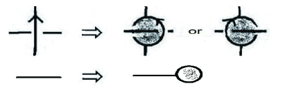
Figure 1: Transformation of an oriented arc diagram into a chord diagram

If two based loops are connected by a chord not meeting the other chords, we can replace it by one based loop (which is also called the chord diagram of an arc diagram) although a carefulness is needed in the calculation of the knotting probability. An example of the procedure to obtain the chord diagram $C(D(L;z_{s}))$ from the projection image $\lambda_{z_{s}}(L)$ of a spatial arc $L$ with $3$ edges of the heights suitable near the triple point is illustrated in Fig. 2, where note that the case of $u=z_{s}$ is easier to construct the chord diagram $C(D(L;u))$ from the projection image $\lambda_{u}(L)$ of a spatial arc $L$.

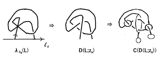
Figure 2: Producing the chord diagram $C(D(L;z_{s}))$ from the projection image $\lambda_{z_{s}}(L)$

Let $D$ be an oriented $n$-crossing arc diagram, and $C(D)$ the chord diagram of $D$. Let $o_{s}$ and $o_{t}$ be the based loops in $C(D)$ transformed from the starting and terminal points $v_{s}$ and $v_{t}$, respectively. There are $(n+2)^{2}$ chord diagrams $A$ obtained from the chord diagram $C(D)$ by joining the loops $o_{s}$ and $o_{t}$ with any based loops of $C(D)$ by two chords not passing the other based loops. A chord diagram obtained in this way is called an adjoint chord diagram of $C(D)$ with an additional chord pair. Note that the ribbon surface-knot $F(C(D))$ of the chord diagram $C(D)$ is a ribbon $S^{2}$-knot and the ribbon surface-knot $F(A)$ of an adjoint chord diagram $A$ is a genus $2$ ribbon surface-knot. A chord diagram is said to be unknotted or knotted according to whether it represents a trivial or non-trivial ribbon surface-knot, respectively.

The idea of the knotting probability is to measure how many knotted chord diagrams there are among the $(n+2)^{2}$ adjoint chord diagrams of $C(D)$. Since there are overlaps among them up to canonical isomorphisms, we consider the $n^{2}+2n+2$ adjoint chord diagrams $A$ of $C(D)$ by removing some overlaps. The $n^{2}+2n+2$ adjoint chord diagrams $A$ of $C(D)$ are classified by the following three types:

x

Type I. Here are the $2$ adjoint chord diagrams of $C(D)$ which are the adjoint chord diagram with two self-attaching additional chords and the adjoint chord diagram with a self-attaching additional chord on $o_{s}$ and an additional chord joining $o_{s}$ with $o_{t}$.

Type II. Here are the $2n$ adjoint chord diagrams $A$ of $C(D)$. The $2n$ adjoint chord diagrams of $C(D)$ are given by the additional chord pairs consist of a self-attaching additional chord on $o_{s}$ (or $o_{t}$, respectively) and an additional chord joining $o_{t}$ (or $o_{s}$, respectively) with a based loop except for $o_{s}$ and $o_{t}$.

Type III. Here are the $n$ adjoint chord diagrams $A$ of $C(D)$ where the additional chord pairs consist of an additional chord joining $o_{s}$ with $o_{t}$ and an additional chord joining $o_{s}$ with a a based loop except for $o_{s}$ and $o_{t}$.

Type IV. Here are the $n(n-1)$ adjoint chord diagrams $A$ of $C(D)$ where the additional chord pair joins the pair of $o_{s}$ and $o_{t}$ with a distinct based loop pair not containing $o_{s}$ and $o_{t}$. x

x

In [9], it is shown that every adjoint chord diagram of the chord diagram $C(D)$ of any $n$ crossing arc diagram $D$ is deformed into one of the adjoint chord diagrams of type I, II, III and IV of the chord diagram $C(D)$. Thus, it is justified to reduce the $(n+2)^{2}$ adjoint chord diagrams to the $n^{2}+2n+2$ adjoint chord diagrams.

The knotting probability $p(D)$ of an arc diagram $D$ is defined to be the quadruple

$$p(D)=(p^{\tiny\mbox{I}}(D),p^{\tiny\mbox{II}}(D),p^{\tiny\mbox{III}}(D),p^{\tiny\mbox{IV}}(D))$$

of the following knotting probabilities $p^{\tiny\mbox{I}}$, $p^{\tiny\mbox{II}}$, $p^{\tiny\mbox{III}}(D)$ of types I, II III, IV.

x

Definition.

(1) Let $A_{1}$ and $A_{2}$ be the adjoint chord diagrams of type I and assume that there are just $k$ knotted chord diagrams among them. Then the type I knotting probability of $D$ is

$$p^{\tiny\mbox{I}}(D)=\frac{k}{2}.$$

(2) Let $A_{i}\,(i=1,2,\dots,2n)$ be the adjoint chord diagrams of type II and assume that there are just $k$ knotted chord diagrams among them. Then the type II knotting probability of $D$ is

$$p^{\tiny\mbox{III}}(D)=\frac{k}{2n}.$$

(3) Let $A_{i}\,(i=1,2,\dots,n)$ be the adjoint chord diagrams of type III and assume that there are just $k$ knotted chord diagrams among them. Then the type III knotting probability of $D$ is

$$p^{\tiny\mbox{III}}(D)=\frac{k}{n}.$$

(4) Let $A_{i}\,(i=1,2,\dots,n(n-1))$ be the adjoint chord diagrams of type IV and assume that there are just $k$ knotted chord diagrams among them. Then the type IIV knotting probability of $D$ is

$$p^{\tiny\mbox{IV}}(D)=\frac{k}{n(n-1)}.$$

x

When the orientation of an arc diagram $D$ is changed, all the orientations of the based loops of the chord graph $C(D)$ are changed at once. This means that the knotting probability $p(D)$ does not depend on any choice of orientations of $D$, and we can omit the orientation of $D$ in figures. See [9] for actual calculations of $p(D)$.

The knotting probability $p(D)$ has $p(D)=1$ if

$$p^{\tiny\mbox{I}}(D)=p^{\tiny\mbox{II}}(D)=p^{\tiny\mbox{III}}(D)=p^{\tiny\mbox{IV}}(D)=1$$

and otherwise, $p(D)<1$. The knotting probability $p(D)$ has $p(D)>0$ if

$$p^{\tiny\mbox{I}}(D)+p^{\tiny\mbox{II}}(D)+p^{\tiny\mbox{III}}(D)+p^{\tiny\mbox{IV}}(D)>0$$

and otherwise, $p(D)=0$.

For an oriented spatial arc $L$ in ${\mathbf{R}}^{3}$, the knotting probability $p(L;u)$ of $L$ for a unit vector $u\in S^{2}$ is defined to be

$$p(L;u)=p(D(L;u))$$

for the arc diagram $D(L;u)$ for $u$. Thus,

$$p^{\tiny\mbox{I}}(L;u) = p^{\tiny\mbox{I}}(D(L;u)),$$

$$p^{\tiny\mbox{II}}(L;u) = p^{\tiny\mbox{II}}(D(L;u)),$$

$$p^{\tiny\mbox{III}}(L;u) = p^{\tiny\mbox{III}}(D(L;u)),$$

$$p^{\tiny\mbox{IV}}(L;u) = p^{\tiny\mbox{IV}}(D(L;u)).$$

Although $p(L;u)$ is unchanged by any choice of a string orientation in the arc diagram level $D(L;u)$, the knotting probability $p(-L;u)$ may be much different from the arc diagram $p(L;u)$ in general, because the arc diagram $D(L;u)$ may be much different from the arc diagram $D(-L;u)$ in general (cf. Corollary 2.4). In any case, the unordered pair of $p(L;u)$ and $p(-L;u)$ is considered as the knotting probability of a spatial arc $L$ independent of the string orientation. When one-valued probability is desirable, a suitable average of the knotting probabilities

$$p^{\tiny\mbox{I}}(\pm L;u),\,p^{\tiny\mbox{II}}(\pm L;u),\,p^{\tiny\mbox{III}}(\pm L;u),\,p^{\tiny\mbox{IV}}(\pm L;u)$$

is considered. For a special spatial arc $L$, we have the following corollary.

x

Corollary 3.1.

(1) If the projection image $\lambda_{u}(L)$ is inbound, then

$$p(L;u)=p(L;-u)$$

for any unit vector $u\in S^{2}$. In particular, if the spatial arc $L$ is inbound, then $p(L;u_{\gamma})=p(L;-u_{\gamma})$ for the front edge vector $u_{\gamma}$.

(2) If $L$ is even, then

$$p(-L;u)=p(L;u)\quad\mbox{or}\quad p(-L;u)=p(L;-u)$$

according to whether the orientations of $P(\ell_{\gamma},\ell_{s})$ and $P(\ell_{\gamma},\ell_{t})$ coincide or not.

x

Proof of Corollary 3.1. In [9], it is shown $p(D)=p(D^{*})$ for an inbound arc diagram $D$ and the mirror image $D^{*}$ of $D$. By Corollary 2.2 (1) and (4), the arc diagrams $D(L;u)$ and $D(L;u_{\gamma})$ are inbound arc diagram with $D(L;-u)$ and $D(L;-u_{\gamma})$ the mirror images. Thus, (1) is obtained. For (2), by Corollary 2.2 (1) and (5), the arc diagram $D(-L;u)$ is isomorphic to the arc diagram $D(L;u)$ or $D(L;-u)$ according to whether the orientations of $P(\ell_{\gamma},\ell_{s})$ and $P(\ell_{\gamma},\ell_{t})$ coincide or not, obtaining the result. $\square$

x

For example, the spatial arc $L$ in Fig. 2 is inbound and even, and we have

$$p(L;z_{s})=p(L;-z_{s})=p(-L,z_{s})=p(-L,-z_{s})=(1,\frac{1}{2},0,0)$$

by Corollary 3.1 where the calculations on the arc diagram $C(D(L;z_{s}))$ are done in Fig. 3 (see [9] for the details of the calculation).

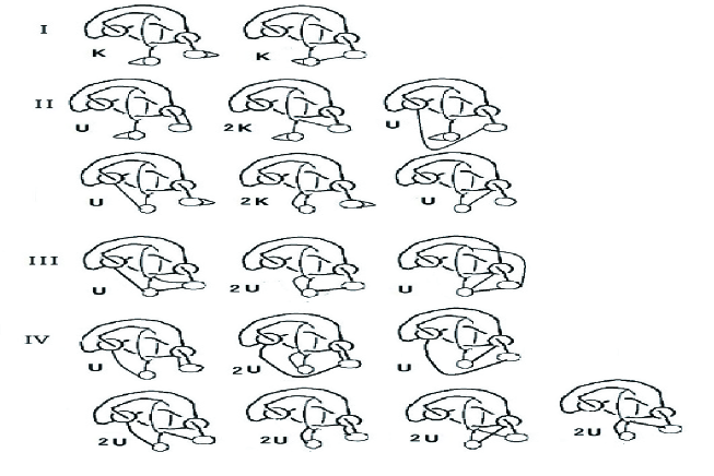
Figure 3: Calculations on the chord diagram $C(D(L;z_{s}))$

x

Acknowledgements. This work was in part supported by Osaka City University Advanced Mathematical Institute (MEXT Joint Usage/Research Center on Mathematics and Theoretical Physics).

x

References

- [1] R. H. Crowell and R. H. Fox, Introduction to knot theory (1963) Ginn and Co.; Re-issue Grad. Texts Math., 57 (1977), Springer Verlag.
- [2] A. Kawauchi, A survey of knot theory, Birkhäuser (1996).
- [3] A. Kawauchi, On transforming a spatial graph into a plane graph, Statistical Physics and Topology of Polymers with Ramifications to Structure and Function of DNA and Proteins, Progress of Theoretical Physics Supplement, 191 (2011), 235-244.
- [4] A. Kawauchi, A chord diagram of a ribbon surface-link, J. Knot Theory Ramifications, 24 (2015), 1540002 (24pp.).
- [5] A. Kawauchi, Knot theory for spatial graphs attached to a surface, Contemporary Mathematics, 670 (2016), 141-169.
- [6] A. Kawauchi, Supplement to a chord diagram of a ribbon surface-link, J. Knot Theory Ramifications, 26 (2017), 1750033 (5pp.).
- [7] A. Kawauchi, A chord graph constructed from a ribbon surface-link, Contemporary Mathematics, 689 (2017), 125-136. Amer. Math. Soc., Providence, RI, USA.
- [8] A. Kawauchi, Faithful equivalence of equivalent ribbon surface-links, J. Knot Theory Ramifications, 27, No. 11 (2018),1843003 (23 pages).
- [9] A. Kawauchi, Knotting probability of an arc diagram. http://www.sci.osaka-cu.ac.jp/ kawauchi/diagramknottingprobability.pdf
- [10] A. Kawauchi, T. Shibuya and S. Suzuki, Descriptions on surfaces in four-space, I : Normal forms, Math. Sem. Notes, Kobe Univ., 10(1982), 75-125; II: Singularities and cross-sectional links, Math. Sem. Notes, Kobe Univ. 11(1983), 31-69.
- [11] T. Yanagawa, On ribbon 2-knots; the 3-manifold bounded by the 2-knot, Osaka J. Math., 6 (1969), 447-164.