Galaxy Structural Analysis with the Curvature of the Brightness Profile

Abstract

In this work we introduce the curvature of a galaxy brightness profile to identify its structural subcomponents in a non-parametrically fashion. Bulges, bars, disks, lens, rings and spiral arms are key to understand the formation and evolution path the galaxy undertook. Identifying them is also crucial for morphological classification of galaxies. We measure and analyse in detail the curvature of $14$ galaxies with varied morphology. High (low) steepness profiles show high (low) curvature measures. Transitions between components are identified as local peaks oscillations in the values of the curvature. We identify patterns that characterise bulges (pseudo or classic), disks, bars and rings. This method can be automated to identify galaxy components in large datasets or to provide a reliable starting point for traditional multicomponent modelling of galaxy light distribution.

1 Introduction

Galaxy formation and evolution are vital to understand the Universe as a whole, for galaxies portray the general structure where they emerged and evolved. Galaxy morphology provides us with a framework on which we describe galaxy structures that are connected with such evolution. The processes that gave birth to bulges, disks, bars, rings, arms, halos, for example, are imprinted in the properties or absence of these features.

Traditional understanding of galaxy formation and evolution encloses, basically, the distinction of the processes that originate elliptical galaxies and classical bulges from the formation of disk dominated/spiral galaxies and pseudobulges. The first mechanism are merger events having violent relaxations and hierarchical clustering (Toomre & Toomre, 1972; Tonini et al., 2016; Naab & Trujillo, 2006; Hopkins et al., 2010). In the merger scenario, it is established that elliptical galaxies are formed by major mergers of spiral galaxies (Burkert & Naab, 2003). In the case of spiral, lenticular and irregular galaxies, first it was supposed that they are a result of formative evolution where rapid violent processes such as hierarchical clustering and merging led to the formation of them (White & Rees, 1978; White & Frenk, 1991; Firmani & Avila-Reese, 2003; Buta, 2013).

The physical properties of the galaxy components also bring relevant information regarding the history of the galaxy. Bulges can be formed by two different ways and therefore separated in two categories: classical originates from violent processes such as hierarchical accretion (Naab & Trujillo, 2006; Hopkins et al., 2010; Gadotti, 2009), are dynamically hot and posses similar properties of elliptical galaxies (Fisher & Drory, 2008); pseudobulges originates from secular evolution through longer times scales where disk material is rearranged by bars and spiral structures in a slow steady process (Wyse et al., 1997; Firmani & Avila-Reese, 2003; Kormendy & Kennicutt, 2004; Athanassoula, 2005; Guedes et al., 2013; Grossi et al., 2018). Characteristics of pseudo bulges are not found in elliptical galaxies and can be similar to those of disks, which are dynamically cold with the kinematics dominated by rotation (Fisher & Drory, 2008). Even so, not all bulges can be clearly labelled as classic or pseudo, for there are bulges that present a mix of properties of the two types (Kormendy & Kennicutt, 2004).

More recently, however, with the increase of computational power, numerical simulations allowed more profound studies on galaxy formation and evolution (Mo et al., 2010; Naab & Ostriker, 2017). Examples of such simulations are Millennium (Springel et al., 2005), EAGLE (Schaye et al., 2015), Illustris (and TNG) (Vogelsberger et al., 2014; Pillepich et al., 2017), Horizon-AGN (Dubois et al., 2014; Kaviraj et al., 2017) (between others). Therefore the principles of the ideas commented above changed slightly and other assumptions raised. For example, to cite few: pseudobulges are formed by secular and dynamical processes (Guedes et al., 2013) which can occur together (e.g. through bar dynamics) (Combes, 2009; Binney, 2013) and also from major mergers (Keselman & Nusser, 2012; Grossi et al., 2018); dark matter haloes can also evolve in terms of two phases (not only by secular evolution), early by major mergers and later by minor mergers (Zhao et al., 2003; Diemand et al., 2007; Ascasibar & Gottlöber, 2008).

Besides of how galaxies and its components forms and evolves, galaxy morphological classifications helps to recognise which processes drive galaxy evolution (Buta, 2013). The first ideas were presented by Reynolds (1920) and later by Hubble (1936), who separated galaxies in classes constituting the Hubble sequence - from early to late types galaxies. Their classification, and the main procedures adopted in the XX Century, were based on visual examination of galaxy images. The classification procedure gained in detail along the years, new parameters and schemes have been introduced but remained based on the visual inspection of the image by an expert (Morgan, 1958; de Vaucouleurs, 1959; van den Bergh, 1960a, b; Sandage, 1961; van den Bergh, 1976; Buta, 2013).

Within this scenario of components as building blocks of galaxy structure, it is relevant to quantify which structures are present in a given galaxy and what is their contribution to the total galaxy light compared to other components. There are several ways to accomplish that, in general by modelling each component in an analytical fashion and then trying a combination of them that best describes the galaxy light distribution (Caon et al., 1993; Peng et al., 2002; Simard et al., 2002; de Souza et al., 2004; Erwin, 2015, among others). This process can describe the galaxy photometry very precisely, however there are some drawbacks. In cases of multicomponent, which are the majority of galaxies, the minimisation data-model is numerically unstable and converges only with the assistance of an experienced user, which limits the range of the model parameters. Furthermore, the joint component models fitted to the galaxy can be degenerate for different combinations of the parameters (e.g. De Jong et al., 2004; Andrae et al., 2011; Sani et al., 2011; Meert et al., 2013), giving the same residuals within the photometric errors, and thus are inconclusive. In some cases leading to situations where they are not physically reasonable.

These restrictions can be overcome with user inspection, as mentioned. Nevertheless, the flood of photometric data that was been made available in the last two decades, for example since the first data release of SDSS (Abazajian et al., 2003) (to cite only one big survey) urged us to reinvent our basic methods and tools to appropriate from all the physical information contained in it. Thus, an automated non-parametric method which can infer the basic properties of the components of a given galaxy could greatly increase the amount of information we could gather from the survey’s data. In this way, we introduce the curvature of the galaxy’s brightness profile ${\kappa}(R)$ with the purpose of inferring the galaxy’s structural components.

The purpose in doing this is that ${\kappa}(R)$ may be used to identify if a galaxy is single or multicomponent, and in this case, it would inform the radial scale length of each component. This is possible because $\kappa$ calculated on the radial profile is a measure of its steepness, and a priori each component has its own steepness. We argue that this new approach is more physically motivated than previously ones because it is independent of parameters. In this paper we are firstly introducing the concept and analysing the results in an non-automated way, the automation and improvements are left for a next paper.

This paper is structured as follows. In Section 2 briefly exposes approaches similar to ours. In Section 3 we introduce our approach for galaxy structural analysis and morphometry using the curvature. In 4 we discuss the data sample used. The application of the technique to the data is carried out in Section 5. In Sections 6 and 7 we discuss and summarize our results, respectively. Also, supplementary material is found in the Appendix Sections. The Appendix A deal with the curvature of a Sérsic profile and Appendix B displays the galaxy images and curvature plots of our analysis related to Section 5.

2 Related Work

Several techniques to distinguish galaxy components have been developed over the years. Basically they are classified whether they perform the modelling in the extracted brightness profile of the galaxy ($1$D modelling) or directly in the galaxy image ($2$D modelling). The most widespread $1$D approach is to fit ellipses to a set of isophotes – an evolution of aperture photometry done at the telescope (Jedrzejewski, 1987; Jungwiert et al., 1997; Erwin & Sparke, 2003; Cabrera-Lavers & Garzón, 2004; Erwin, 2004; Laurikainen et al., 2005; Gadotti et al., 2007; Pérez et al., 2009).

For each isophote there is a collection of geometric and physical parameters that describe it, including the brightness profile (energy flux as a function of distance) which is later used to compare to a model of the components of the galaxy. As a side effect, this technique is often used to identify behaviour in the parameters (ellipticity, position angle, Fourier coefficients of the ellipse expansion) that may indicate the domain of different components or, in another context, to give hints of ancient interactions, mergers or cannibalism. Also with a similar purpose, other non-parametric approaches like unsharp masking (Malin, 1977; Erwin & Sparke, 2003; Kim et al., 2012) and structure maps (Pogge & Martini, 2002; Kim et al., 2012) are used.

Unidimensional techniques are better suited to extract geometric information of individual isophotes, but incorporating the instrument response function (the PSF – point spread function) is not trivial. Moreover, there is no consensus on which distance coordinate to use to extract the profile – major or minor axis or different combination of both – whose choice impacts the leading parameters (Ferrari et al., 2004). Two-dimensional algorithms operate directly in the galaxy image, so there is no ambiguity in extracting the brightness profile. Real PSFs can be incorporated in the models and the process (convolution) in this conserves energy. Their disadvantage are the high computational cost – not so critical nowadays – and the instability to initial conditions. This instability increases wildly with the number of components and free parameters in the models. In some situations (e.g. a combination of bulge, bar and disc), the algorithm only converges if the initial parameters are very close to the final ones, which makes the algorithm itself unnecessary (see for example Haussler et al., 2007).

Regardless the method, $1$D or $2$D, the galaxy is then modelled with a combination of components, usually described with a Sérsic function (Sérsic, 1968) with different $n$, scale lengths and intensity to resemble a bulge, a disk, a bar and so on. (See for example Caon et al., 1993; Peng et al., 2002; de Souza et al., 2004; Laurikainen et al., 2005; Gadotti, 2008; Simard et al., 2011; Kormendy & Bender, 2012; Bruce et al., 2014; Argyle et al., 2018; Erwin, 2015, and references therein).

The curvature itself, as far as we know, has not been used in the context of galaxy structural analysis, nevertheless it has been used in different fields of science in a similar manner. In medicine, for example, it is used to recognize the existence of breast tumours (Lee et al., 2015), where it is applied on the imaging data of the photograph of each patient’s breast in order to classify the tumours. Luders et al. (2006) used the curvature to study the process of brain gyrification according genre, a process present on the cerebral cortex which forms folds, composed by peaks and valleys (see their methodology for details). They have used the mean curvature as a external measure of how the normal vector of the surface of the brain changes across it. The idea behind it is similar to ours, because here the curvature $\kappa(R)$ specifies how the normal vector of $I(R)$ changes along radius, giving information of what kind of component is present in each specific region of the profile. Other works using curvature were found on dental studies (Zhang, 2015; Destrez et al., 2018) and in general medicine (Preim & Botha, 2014).

In summary, we intend that the curvature may be used as a non-parametric tool to identify different galactic components and constrain their scale lengths. This might support the structural analysis made with standard procedures commented above. For example: instead of force arbitrarily multiple Sérsic functions in structural decompositions, the results from curvature might provide an initial estimate about the morphology of each component and their scale lengths; also it can be comparable with the results obtained from the ellipse fitting technique, where properties are also extracted under the variation of position angle and ellipticity along radius, since these may change between different components.

3 Curvature of the brightness profile

3.1 Definitions

With the purpose to identify galaxy substructures non-parametrically we introduce the curvature of the brightness profile ${\kappa}(R)$. The concept of curvature comes from differential geometry (e.g. Tenenblat, 2008): given a function $f=f(x)$ it is possible to measure how it deviates from a straight line (the same reasoning can be extended to higher dimensional spaces) by means of a curvature measure on $f$, that is $\kappa[f(x)]\equiv\kappa(x)$.To clarify these concepts of curvature, consider Fig. 1. Along the path $S$, at each different point $P$ we can draw a circle with radius $\mathcal{R}$ passing through it and its neighbour points. This circle is called of osculating circle. The measure of curvature of the path at point $P$ is inversely proportional to the osculating circle of radius $\mathcal{R}$ bypassing through that same point whose surface normal vector points towards to the centre of the circle, that is $\kappa\propto 1/\mathcal{R}$ (see also additional schematics in Crane et al., 2013; Lee et al., 2015). Along the path, we can understand how changes the curvature of different points from $P$ to $P^{\prime}$ drawing many osculating circles with radii $\mathcal{R}$ and $\mathcal{R}^{\prime}$ as we move along the path. In Fig. 1, at $P$ the curvature is negative and small because $\mathcal{R}$ is large; at $P^{\prime}$ the curvature $\kappa^{\prime}$ is positive and larger than $\kappa$ because $\mathcal{R}^{\prime}$ is small; at $P^{\prime\prime}$ the curvature tends to zero because $\mathcal{R}^{\prime\prime}$ goes infinite (we have not draw the corresponding circle).

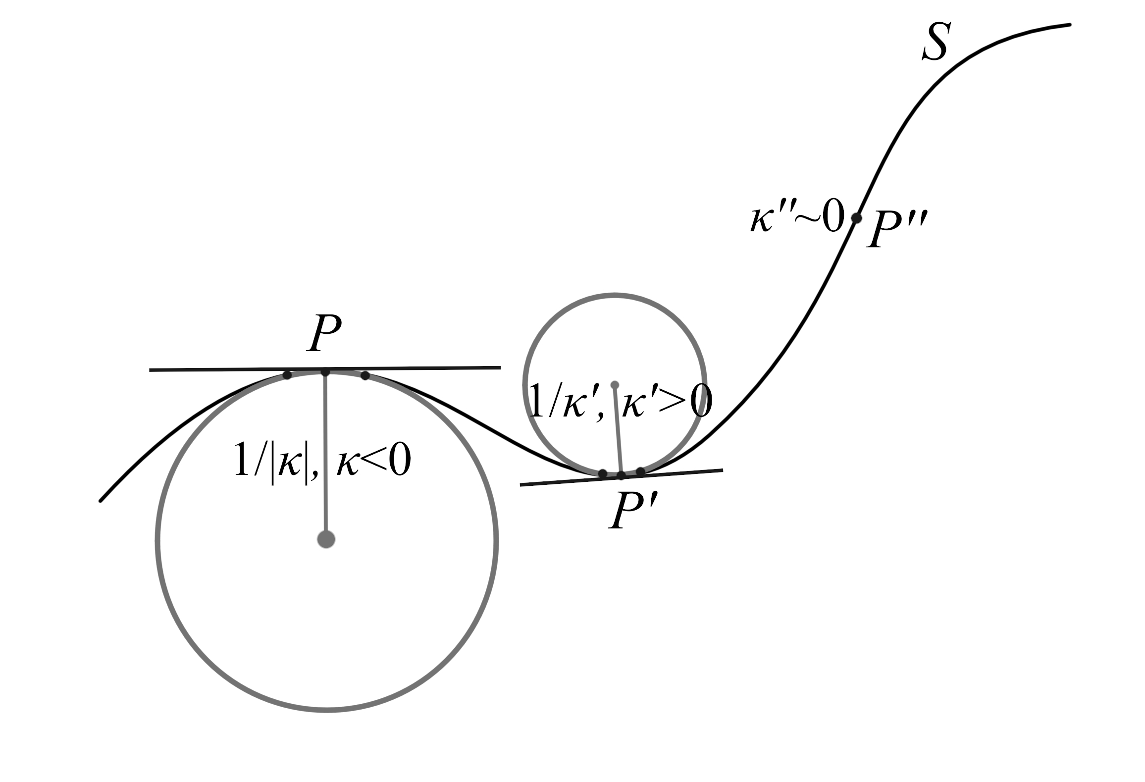
Figure 1: Idealized graphical representation of how the curvature is measured along a path $S$ at different points $P$, $P^{\prime}$ and $P^{\prime\prime}$. At each point an osculating circle with radius $\mathcal{R}$ can be drawn so that $\kappa\propto 1/\mathcal{R}$.

In this work we take $f(x)$ to be the radial brightness profile $I(R)$ of the galaxy (more details below). From the curvature’s definition of a path (e.g Tenenblat, 2008) we have

$$\kappa(R)=\dfrac{\dfrac{d^{2}I(R)}{dR^{2}}}{\left[1+\left(\dfrac{dI(R)}{dR}\right)^{2}\right]^{3/2}}.$$ (1)

Equation (1) is a particular case when we have a one-dimensional continuous function. However, in this work we will deal with non-continuous quantities, which are the discrete data of light profiles of the galaxies. Therefore, we seek for a discrete curvature measure on our data which involves numerical operations. For two discrete vectors representing two quantities, say $I$ and $R$, the curvature is defined as

$$\kappa=\frac{\delta R_{i}\delta^{2}I_{i}-\delta I_{i}\delta^{2}R_{i}}{(\delta R_{i}^{2}+\delta I_{i}^{2})^{3/2}}$$ (2)

where $\delta$ represents the numerical differentials (derivatives) between the discrete $i$-values of $R$ and $I$.

As commented previously, the curvature is inversely proportional to the osculating circle respective to a point $P$ in a path $S$. This means that in any arbitrary scale, both $x$-axis and $y$-axis variables must have the same scale for our interpretation. In other words, the variation of $x$ and $y$ must be represented in a space whose metric preserves its components or properties. Therefore, for practical purposes, it is convenient to use an orthonormal referential system, consequently we can trace an osculating circle for a set of points in relation to a centred point $P$ in the path $S$ represented in this orthonormal system. Otherwise we would have an ellipse instead of a circle, and the interpretation will be different since it is not possible to draw an osculating circle in the $x-y$ space with different scales.

Therefore, having two quantities which does not have the same physical meaning and with different scales, such as intensity $I$ and radius $R$, it is necessary to transform them into a space having equal metric. The orthonormal system is obtained with a normalization of equations (1) and (2), that is to confine both $I(R)$ and $R$ to vary in the unitary interval $[0,1]$.

Before we proceed to the normalization, there is a particular result from the curvature for we should take into account: it is zero for a straight line ($\text{d}f/\text{d}x=0$) and non zero for other general cases. A galactic disk generally follow an exponential profile (Freeman, 1970) (see Appendix A). Then in log space, this profile is a straight line and we can conclude that the curvature of a disk in log space is close to zero. With this in mind we argue that is more useful to normalize the logarithm of $I(R)$, $\log[I(R)]$, instead of $I(R)$. Our point is that we will be able to easily distinguish disks from non disks using $\kappa$. Hence a normalization $\nu(R)$ for $\log[I(R)]$ in the range $[0,1]$ can be written as

$$\nu(R)\equiv\frac{\log[I(R)]-\min(\log I)}{\max(\log I)-\min(\log I)}.$$ (3)

The next step is the normalization for $R$. We need to change the variation of the dimensional variable $R$ to another quantity that is dimensionless and confine it in the range $[0,1]$. Generally, observations do not reach the faintest parts of a galaxy, so it is usual to define a galaxy size. One common choice is the Petrosian radius $R_{p}$ (Petrosian, 1976), defined by the radius where the Petrosian function

$$\eta(R)=\frac{\Braket{I}(R)}{I(R)}$$ (4)

has a definite value, i.e.

$$\eta(R_{p})=\eta_{0}.$$ (5)

Here $\Braket{I}(R)$ is the mean intensity inside $R$ and $I(R)$ the intensity at $R$. Following (Bershady et al., 2000; Blanton et al., 2001; Ferrari et al., 2015) we use $\eta_{0}=5$ with $2R_{p}$ as the size of galaxy. The normalization of $R$ now reads

$$\chi=\frac{R}{2R_{p}}.$$ (6)

With this normalization at $2R_{p}$, we also set that the value of $\min(\log I)$ in equation (3) becomes $\min(\log I)\sim\log I(2R_{p})$ under the assumption that the profiles generally always decreases as $R$ increases.

Now, the curvature in terms of normalized variables measures the rate of change of $\nu(R)$ in terms of the new variable $\chi$. So the complete normalized curvature is obtained taking the derivative of $\nu(R)$ with respect to $\chi$. The relationship between the differentials of $\text{d}R$ and $\text{d}\chi$ is

$$\text{d}\chi=\frac{\text{d}R}{2R_{p}}.$$ (7)

Taking the first and second derivatives,

$$\frac{\text{d}\nu}{\text{d}\chi}=2R_{p}\frac{\text{d}\nu}{dR}\qquad{\rm and}\qquad\frac{\text{d}^{2}\nu}{\text{d}\chi^{2}}=4R_{p}^{2}\frac{\text{d}^{2}\nu}{\text{d}R^{2}}$$ (8)

we obtain the normalized curvature as

$$\widetilde{\kappa}(R)=4R_{p}^{2}\dfrac{\text{d}^{2}\nu}{\text{d}R^{2}}\left[1+4R_{p}^{2}\left(\dfrac{\text{d}\nu}{\text{d}R}\right)^{2}\right]^{-3/2}.$$ (9)

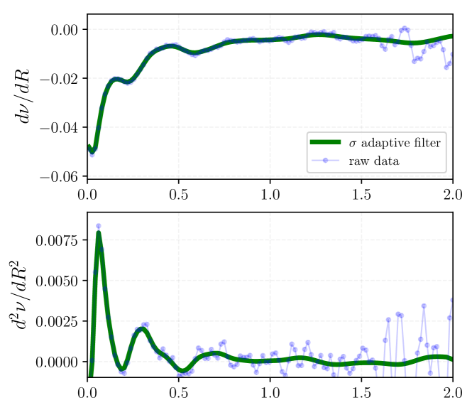
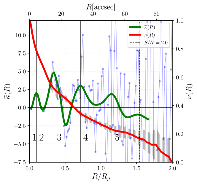
Figure 2: Example of the procedure to calculate $\widetilde{\kappa}(R)$ for the EFIGI/SDSS data of galaxy NGC 1211/PGC 11670. Top: first derivative of $I(R)$, raw (blue) and filtered (green). Middle: the same but for the second derivative of $I(R)$. Bottom: log-normalized brightness profile $\nu(R)$ (red) and the raw (blue) and filtered (green) curvature. The filter is discussed in Section 3.3. The solid vertical lines represent the possible transition between regions dominated by different components, and will be explained latter on Section 5.1. The vertical dashed line delimit the regions where the signal-to-noise $S/N$ goes below $2$ and we avoid to interpret profiles outside that region.

Returning to the discrete case in Eq. (2), the discrete normalized curvature in terms of the new variables is, according to the new normalized variables, simply

$$\widetilde{\kappa}=\frac{\delta\chi_{i}\;\delta^{2}\nu_{i}-\delta\nu_{i}\;\delta^{2}\chi_{i}}{\left(\delta\chi_{i}^{2}+\delta\nu_{i}^{2}\right)^{3/2}}.$$ (10)

As an example, Fig. 2 shows $\widetilde{\kappa}$ measured for the EFIGI galaxy NGC 1211/PGC 11670, together with the normalized profile $\nu(R)$ and the related derivatives of $\nu(R)$ (raw and filtered, see Section 3.3) used to calculate the curvature.

The rationale behind using the brightness profile curvature $\widetilde{\kappa}$ to identify structural subcomponents in galaxy light is based on the fact that the curvature of disks will be null whilst that of bulges will be positive and dependent on its Sérsic index; regions highly affected by the PSF would tend to be negative in $\widetilde{\kappa}$; the transition between different components would be manifested in curvature changes; galaxies with disks (either inner or outer) will present $\widetilde{\kappa}$  that are zero over the region dominated by the disk (see next section). In Appendix A we use equation (9) to work out the expressions for the curvature of Sérsic profile models. In Section 5 we develop this concepts in practice examining how $\widetilde{\kappa}$ behaves for different combinations of galaxy subcomponents.

3.2 Measuring $I(R)$ with Morfometryka

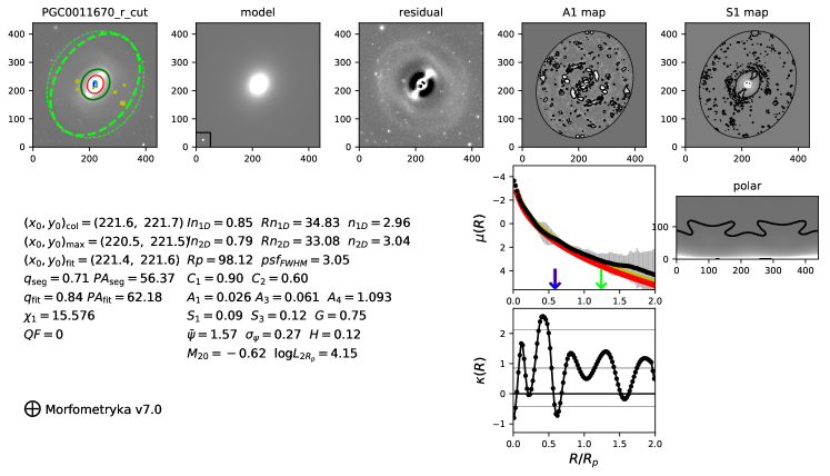
Figure 3: Output from mfmtk for the SDSS $r$ image of NGC1211. The top panel shows (from left to right) the galaxy image, a single Sérsic fits model, residual image, and the asymmetry $A_{1}$ and smoothness $S_{1}$ maps. The numerical quantities are related to photometry and morphometry. The Sérsic parameters used to the model are the ones with the $2D$ index, performed in a two dimensional modelling (see Ferrari et al., 2015). The bottom right panel displays the surface brightness profile $\mu(R)$, the curvature $\widetilde{\kappa}(R)$ and the polar plot used for $\sigma_{\psi}$.

The brightness profile is measured as part of the processing done by Morfometryka (Ferrari et al., 2015). Morfometryka is an algorithm designed to perform several photometric and morphometric measurements on a galaxy image in an automated way with no user interaction. The inputs are the galaxy image stamp and respective point spread function (PSF) image. It then measures the background in an iterative way, segmentates the image – separating galaxy, other objects and background – and measure basic geometric parameters of the segmented region, like the centre, the position angle, major and minor axis (see Fig. 3 for an example of an output result from Morfometryka). Based on this information, it performs aperture photometry on similar ellipses from the centre up to 2$R_{p}$ (the Petrosian radius), spaced 2 pixel apart and having the width of 1 pixel. The brightness profile $I(R)$ is the azimuthally averaged value of the ellipses aforementioned; the error is the standard deviation of the same pixel set.

3.3 The Filters for $\widetilde{\kappa}(R)$

Measuring the curvature, according to Eq. (1), would be just a matter of evaluating the first and second derivatives of the brightness profile. In practice, with discrete points for $I(R)$ contaminated by noise, the direct estimation of $\text{d}\nu/\text{d}R$ and $\text{d}^{2}\nu/\text{d}R^{2}$ is worthless because the noise in $I(R)$ is amplified by the derivative operator (a high pass filter). Fig. 2 shows this noise magnification that yield a very scattered curvature (blue points).

One way to overcome the limitations imposed by the noise is to use a filter to enhance the signal-to-noise of the data. Many linear filters attenuate the signal as well as the noise. For our purpose, we need a filter that attenuates the noise but keeps the overall structure present in the data. In general, the signal-to-noise ratio is higher in inner regions of the galaxy data and decreases to outermost regions. Therefore, the best solution to use in the filtering task is an adaptive filter, which takes into account the level of the dispersion and adapts the level of the smoothing accordingly.

We adopt a simple adaptive Gaussian filter $G$, which changes the Gaussian dispersion $\sigma$ according to the local signal to noise ratio. We write a linear relation between $\sigma$ and the radial distance $R$, assuming that inner regions are less noisy and constituted by small structures, and outer regions, more noisy and large structures, which is true for the majority of galaxies. We then write

$$\sigma(R)=\left(\sigma_{\max}-\sigma_{\min}\right)\frac{R}{2R_{p}}+\sigma_{\min}$$ (11)

where $\sigma_{\min}$ is the standard deviation of the filter at the centre of the data and $\sigma_{\max}$ in the outermost region. Generally $\sigma_{\min}\lesssim 2$ and $\sigma_{\max}\sim 0.1\times(2R_{p})$. We performed tests with this design and verified that a single step of filtering in $\nu(R)$ is enough to remove effectively the noise from the data; to overcome edge effects caused by the filter when smoothing points at the edges, we discard the points corresponding to $2\sigma_{\rm min}$ at the beginning and $2\sigma_{\rm max}$ and the end of $\widetilde{\kappa}$ – note that the green line of $\widetilde{\kappa}(R)$ in Fig. 2 ends at $R/R_{p}\sim 1.7$.

4 Data Sample

The data in the present study is constituted by galaxies that already have been studied in terms of structural decompositions and multicomponent analysis. We have selected galaxies contained in the following works (Wozniak & Pierce, 1991; Prieto et al., 2001; Cabrera-Lavers & Garzón, 2004; Lauer et al., 2007; Gadotti et al., 2007; Gadotti, 2008, 2009; Compère et al., 2014; Salo et al., 2015; Gao & Ho, 2017; Yıldırım et al., 2017) (individual references bellow). The data were extracted according to their availability in NED and other databases. These are: EFIGI sample (Baillard et al., 2011), Hubble Space Telescope Archive (HLA), SPITZER Telescope (Dale et al., 2009), Pan-STARRS-1 telescope (Chambers et al., 2016) and Cerro Tololo Inter-American Observatory 1.5m (CTIO$1.5$m) telescope.

Tab. 1 introduces the following information for each galaxy: the complete references, where the data was taken, the filter used and the morphological classification found in the literature. Most of galaxies are in the $r$ band, corresponding to a wavelength around $6250$ angstroms. For the HST images we have the filter f160w, which corresponds to the $H$ band with a wavelength peak of $1.545$ microns. For the Spitzer galaxy NGC 1357, the filter correspond to the IRAC3.6 band with a wavelength around of $3.6$ microns. We have limited our study to a small set of 14 galaxies in order to perform a careful analysis with the curvature. We selected galaxies in each general morphology: ellipticals, lenticular, disk/spiral (with and without bar).

The sample cover the following diversity:

1. galaxies with complex structure, e.g. bars, rings, arms, disks, which are notably seem: NGC 1211 (Buta, 2013), NGC 0936 (Wozniak & Pierce, 1991), NGC 1512 (Laurikainen et al., 2006; Compère et al., 2014), NGC 7723 (Prieto et al., 2001);

2. galaxies with fine structures, e.g. core, smooth bars or arms + S0 galaxies with smooth disks which barely can be identified: NGC 0384 (Yıldırım et al., 2017), NGC 1052 (Lauer et al., 2007), NGC 2767 (Nair & Abraham, 2010; Yıldırım et al., 2017), NGC 4267 (Wozniak & Pierce, 1991), NGC 4417 (Kormendy & Bender, 2012), NGC 1357 (Gao & Ho, 2017), NGC 2273 (Cabrera-Lavers & Garzón, 2004), NGC 6056 (Tarenghi et al., 1994; Prieto et al., 2001);

3. galaxies with well known structure in shape, for example ellipticals: NGC 472, NGC 1270 (Yıldırım et al., 2017).

With this set we investigate the behaviour of $\widetilde{\kappa}(R)$ for each representative morphology, recognizing how the curvature differs between each type.

Table 1: Data sample used in this work.

$i$	Galaxy Name + filter	Morphology	Origin	Reference of the data
1	NGC0384-f160w	S03/E1,2	HST	(Yıldırım et al., 2017)
2	NGC0472-f160w	VY CMPT2	HST	(Yıldırım et al., 2017)
3	NGC0936-$r$	SB04	EFIGI	(Baillard et al., 2011)
4	NGC1052-$r$	E1,5(+core6)/S05	EFIGI	(Baillard et al., 2011)
5	NGC1211-$r$	SB0/a(r)7	EFIGI	(Baillard et al., 2011)
6	NGC1270-f160w	E1/VY CMPT2	HST	(Yıldırım et al., 2017)
7	NGC1357-3.6$\mu$m	SA(s)ab1	SPITZER	(Dale et al., 2009; Sheth et al., 2010)
8	NGC1512-$r$	SB(r)a1	CTIO	(Meurer et al., 2006)
9	NGC2273-$r$	SB(r)a1	Pan-STARRS	(Chambers et al., 2016)
10	NGC2767-$r$	E1/S08	HST	(Yıldırım et al., 2017)
11	NGC4267-$r$	S03/SB04,5	EFIGI	(Baillard et al., 2011)
12	NGC4417-$r$	SA0a9	EFIGI	(Baillard et al., 2011)
13	NGC6056-$r$	SB(s)01,10/S0/a11	EFIGI	(Baillard et al., 2011)
14	NGC7723-$r$	SB(r)b1,10	Pan-STARRS	(Chambers et al., 2016)
1 (de Vaucouleurs et al., 1991).
2 (Yıldırım et al., 2017).
3 (Nilson, 1973).
4 (Wozniak & Pierce, 1991).
5 (Sandage & Tammann, 1981).
6 (Lauer et al., 2007).
7 (Gadotti et al., 2007).
8 (Nair & Abraham, 2010).
9 (Kormendy & Bender, 2012).
10 (Prieto et al., 2001).
11 (Tarenghi et al., 1994).

5 Applications to The Data Sample

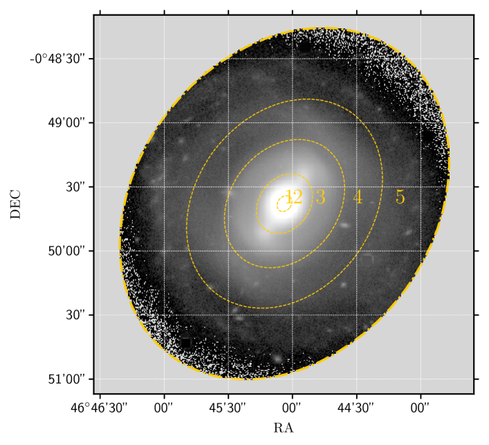
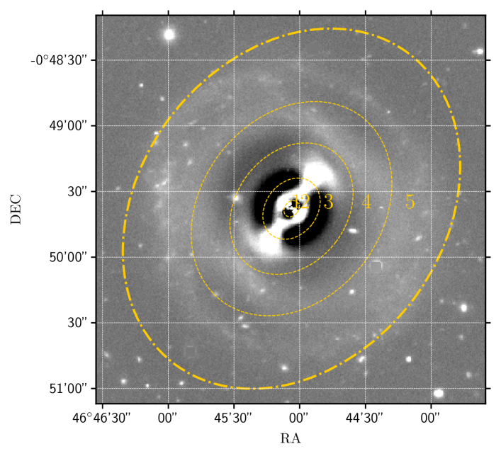
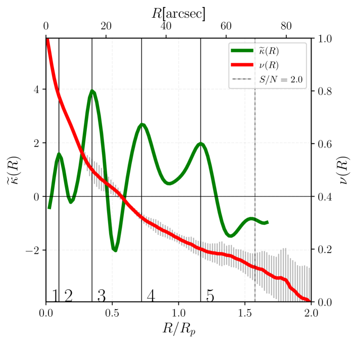
Figure 4: Top: SDSS $r$ image for NGC1211 from the EFIGI sample. The yellow lines represent each component of the galaxy. These regions were drawn from the local peaks in the green line of $\widetilde{\kappa}(R)$ (see bellow). The numbers in the yellow ellipses and in the $\widetilde{\kappa}$ plots refer to the same regions. Middle: Residual from a single Sérsic fit to the image above made with Morfometryka. For both, yellow dotted lines correspond to regions identified in the curvature plot below; yellow dot-dashed line is the $2R_{p}$ region. Bottom: Normalized log-brightness profile (red curve) and curvature $\widetilde{\kappa}$ calculated from it (green curve). The solid vertical lines delimit regions of different components (see text for details). The vertical dashed line is the limit of confidence of SNR=2.

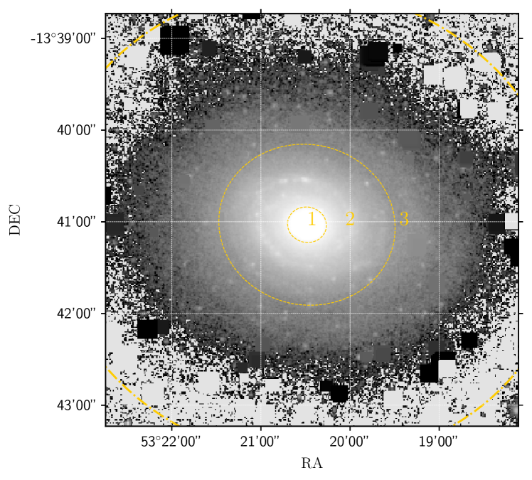
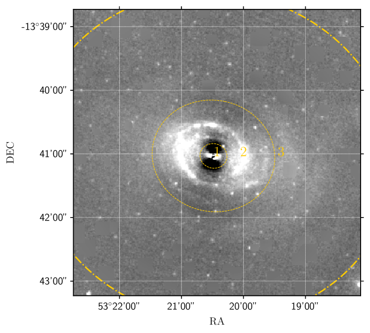
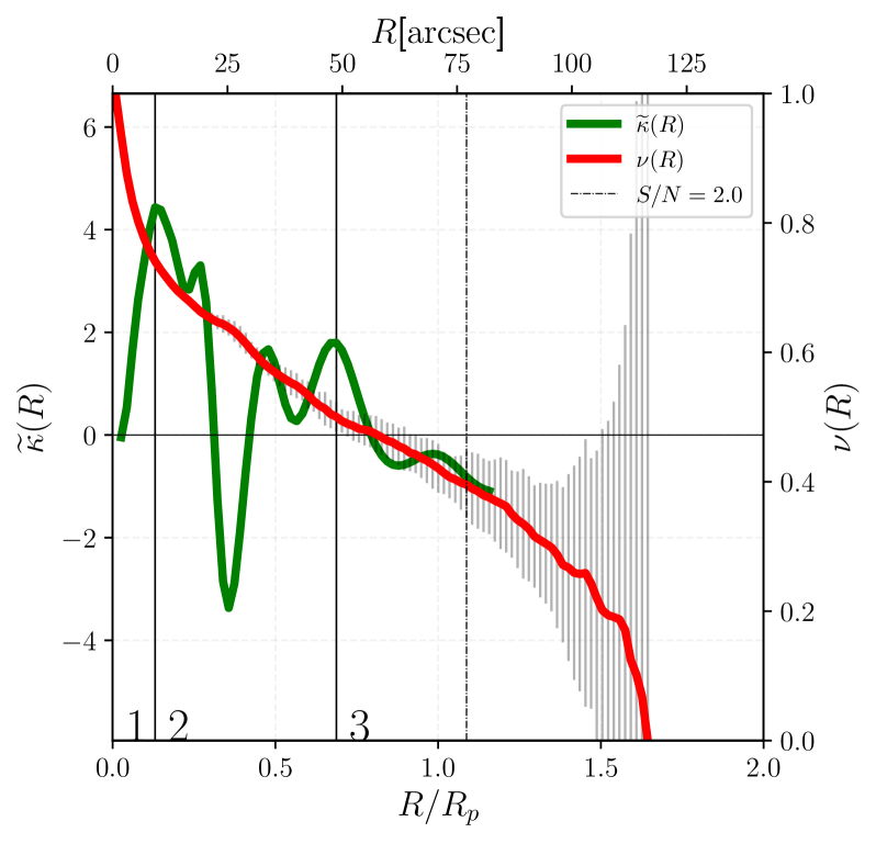
Figure 5: Near infrared band ($3.6\mu$m) of NGC 1357 from Spitzer telescope. Labels and graphic positions are the same as Fig. 4, and the same for the remaining figures. Region 1 is the bulge (high and large peak in $\widetilde{\kappa}$ ). Region 2 is the disk with spiral arms and the outer disk is region 3 with low values in curvature. Again, the dashed vertical line (SNR=2) is our limit of confidence. See the text for further details of this galaxy.

We trace the behaviour of $\widetilde{\kappa}(R)$ for galaxies presented in Tab. 1 with the aim to distinguish galaxy multicomponents and decipher different morphologies. Each galaxy in our sample will be discussed individually in separated sections, divided by their global morphologies, e.g. lenticulars (Section 5.3), spirals (Section 5.4) and ellipticals/spheroidal components (Section 5.5). We begin by discussing $\widetilde{\kappa}$ for two cases in detail: NGC 1211 and NGC 1357. The full data sample is discussed below. The complete set of figures for the curvature are given in the Appendix A.

For each galaxy (see the model reference Fig. 4), we present the broad band image of the galaxy in the top panel. In the middle panel we show the residual map from a single Sérsic fit to the broad band image made with Morfometryka – for the structures are easily visualized on it. For both, yellow dotted lines correspond to regions identified in the curvature plot and yellow dot-dashed line mark the $2R_{p}$ region. The bottom panel shows the normalized brightness profile $\nu(R)$ (red curve – scale in the axis at right) and curvature $\widetilde{\kappa}(R)$ calculated from it (green curve – scale on axis at left). The solid vertical lines delimit regions of different components (discussed below for each galaxies); they correspond to the yellow ellipses in the images, but are inferred from the $\widetilde{\kappa}$ behaviour. The vertical dashed line found in more external regions is the limit of confidence of $\mbox{SNR}=2$.

5.1 Case Study 1: Curvature of NGC 1211

We begin by analysing $\widetilde{\kappa}$ and components from NGC 1211 (PGC 11670) galaxy of the EFIGI sample. It is classified as (R)SB(r)0/a (de Vaucouleurs et al., 1991), i.e. barred spiral/lenticular with rings. Fig. 4 shows the SDSS galaxy $r$ image (top), the residual from a single Sérsic fit by Morfometryka (middle) and the curvature $\widetilde{\kappa}$ (bottom). Changes in $\widetilde{\kappa}$ are related to the transition between regions dominated by different components. In the galaxy image on the top panel, the size of the yellow dotted ellipses overlaid were determined by the local peaks in the curvature plot (bottom), which are signalled as vertical black solid lines in the curvature plot. They delimit regions (identified by numerical labels) that are dominated by different components.

Starting from the central region, we have two local peaks in $\widetilde{\kappa}$ at $R/R_{p}\sim 0.1$ and $R/R_{p}\sim 0.3$. The first region (label 1) seems to be a small structure inside the bulge which is represented by region 2. However, both components have small values in curvature compared to the maximum amplitude ($\widetilde{\kappa}\sim 4$ at $R/R_{p}\sim 0.4$), the bulge in region 2 reaches values close to zero, therefore this indicates that the Sérsic index of this component is close to 1 (this can also be seen by the straight brightness profile in the region – red curve in bottom plot). This may indicate that the bulge of NGC 1211 is a pseudobulge. Note also that the innermost component also has a small $\widetilde{\kappa}$. In Méndez-Abreu et al. (2018) they comment that NGC 1211 has an internal structure called “barlenses”, which is a component different of a bulge contained inside the bar (Laurikainen et al., 2010). Gadotti et al. (2007) also observed a nuclear structure in this galaxy. Therefore, the signature in $\widetilde{\kappa}$ in regions 1 and 2 are not of a classical bulge, but indicate the presence of the nucleus and a pseudobulge.

The second peak at $R/R_{p}\sim 0.3$ is the transition between the bulge and the bar+inner ring – a narrow and negative valley in $\widetilde{\kappa}$. Usually, bars and inner rings are associated with narrow valleys in $\widetilde{\kappa}$. For inner rings they are negative (as will be seen further) and for bars they can be negative or not, but in general both have narrow valleys. The third peak at $R/R_{p}\sim 0.75$ defines the end of the bar and the start of the outer region of the galaxy, label 4 and 5. The transition $4\to 5$ is indicated by the local peak at $R/R_{p}\sim 1.2$. Intermediate regions in 4 shows $\widetilde{\kappa}\sim 0$ regarding a disk like structure. As indicated by Buta (2013), NGC 1211 has two outer rings: i) an inner outer ring identified to be red; ii) an outer outer ring identified to be blue (see his Figure 2.30).

5.2 Case Study 2: Curvature of NGC 1357

NGC 1357 is a non-barred spiral galaxy classified as SA(s)ab (de Vaucouleurs et al., 1991). Gao & Ho (2017) considered that the galaxy has two disks: an inner blue disk which contains well defined spiral arms, and an outer red disk with no spiral arms. Fig. 5 shows the curvature for NGC 1357.

The bulge is indicated by the region of high curvature (1); the valley at (2) is related to the tight shape of the spiral arms, having a ring-like shape, pointed out by Gao & Ho (2017). We found that a high and narrow negative gradient in curvature is characteristic of ring and bar components – which corresponds to Sérsic index lower than unity. The transition of this ring with the spiral structure corresponds to the middle inwards part of region 2. However, all spiral structure is contained inside region 2 which is the inner disk.

The transition between the inner and the outer disk is underpinned by the decrease in the oscillations after the local peak at $R/R_{p}\sim 0.65$, therefore region 3 corresponds to the outer disk with no spiral arms. As mentioned before, a disk has values of $\widetilde{\kappa}$ close to zero. In the following Section we extend the same analysis for the rest of the sample, separating them according to each morphological type. The remaining the figures are in Appendix B.

5.3 Lenticular Galaxies

Lenticular galaxies are at first order composed by a bulge+disk structure and sometimes having a bar, and the bulge can be often classical or pseudo. These kind of galaxies are a suitable tool to use the curvature in order to unveil the nature of the bulge, since the the slope of the light profile is related with such morphologies (Laurikainen et al., 2016). For classical bulges, in principle the higher the slope (high Sérsic index $n$) the higher the curvature. On the other hand, for pseudo, lower slopes (and $n$) may imply lower curvatures. Therefore, analysing the bulge region with $\widetilde{\kappa}$ enables one more way to characterize its morphology.

NGC 936

NGC936 is classified as barred lenticular galaxy SB0 (Wozniak & Pierce, 1991), formed by a structure of bulge+bar+disk. In Fig. 8 we infer from $\widetilde{\kappa}$ that the bulge dominates region 1, while the bar becomes dominant in region 2 – highlighted by the straight valley and negative $\widetilde{\kappa}$. The bar ends close to $R/R_{p}\sim 0.5$. Its properties were also extracted by Muñoz-Mateos et al. (2013), regarding the bar length, they provide $\leavevmode\nobreak\ 50$arcsec.The peak in $\widetilde{\kappa}$ at $R/R_{p}\sim 0.5$ ($\sim 54$arcsec) indicating the end of the bar seems to be in agreement with the outer limit found by the authors (see their figure 3). The bar of NGC 936 was also studied by Erwin & Sparke (2003) together with a nuclear ring inside the bar region. Returning back to the inner component, $\widetilde{\kappa}$ is nearly constant and $\widetilde{\kappa}\sim 1$ (small value compared to the maximum amplitude of $\widetilde{\kappa}\sim 10$). This suggest that the inner region is not a classical bulge, but rather being a pseudobulge – which also may contain a nuclear ring.

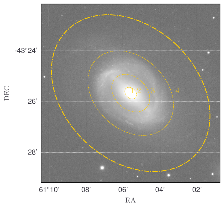
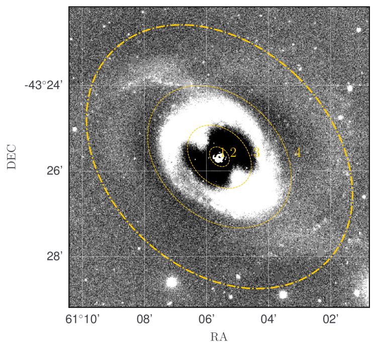
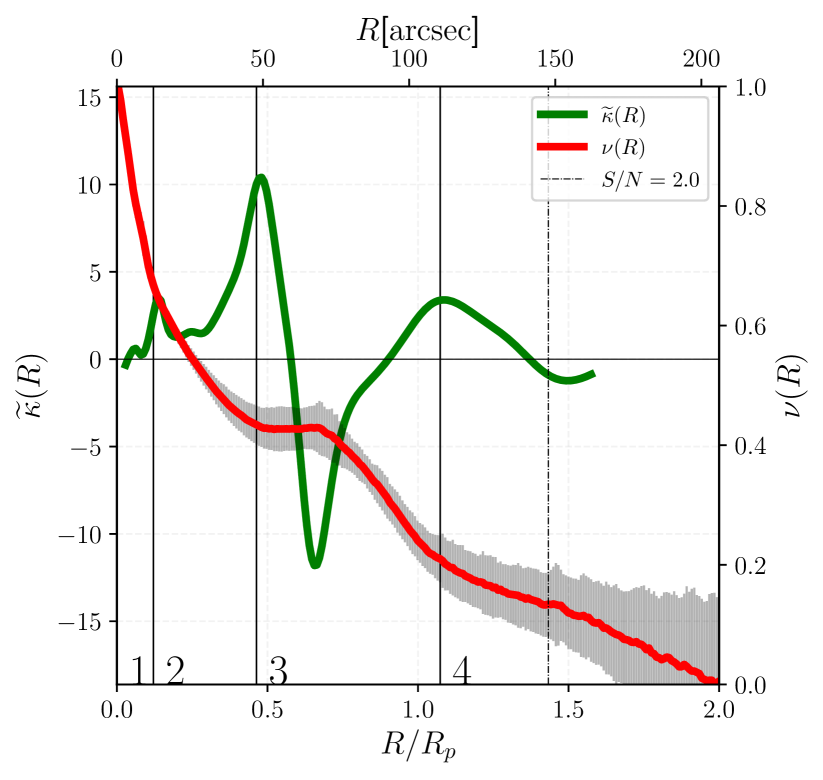
Figure 12: The same as Fig. 4, but for $r$ band of NGC 1512 from CTIO telescope.

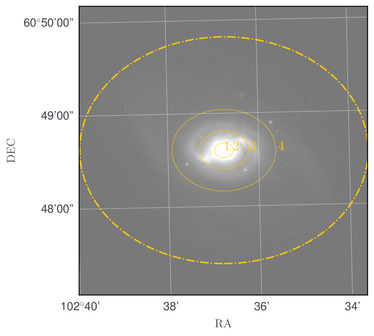
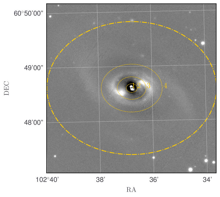
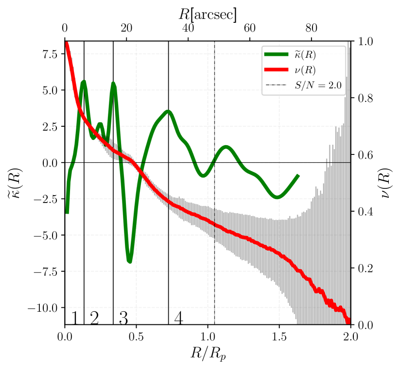
Figure 13: The same as Fig. 4, but for $r$ band of NGC 2273 from Pan-STARRS.

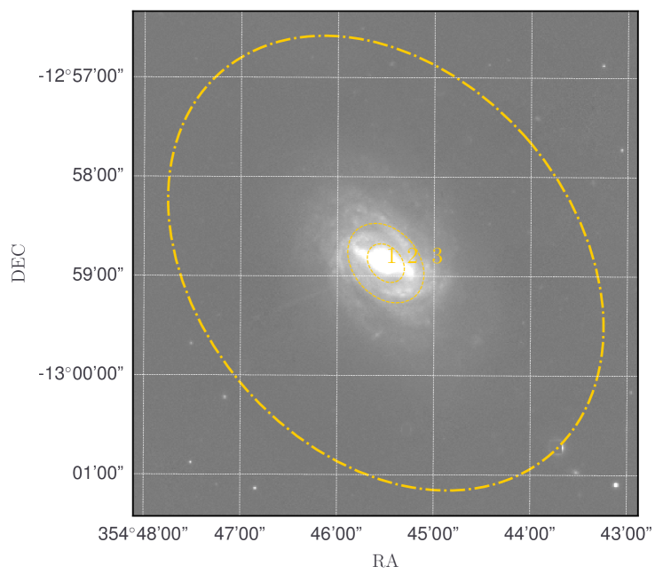
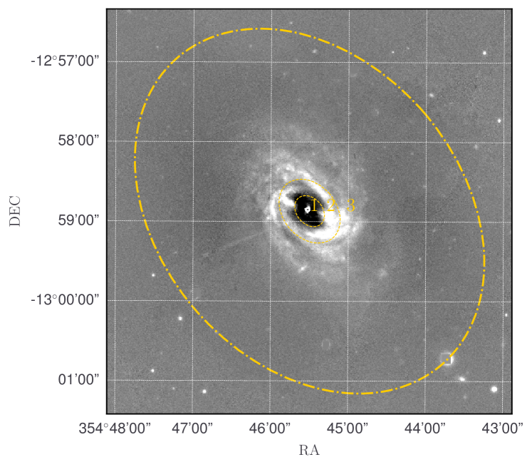
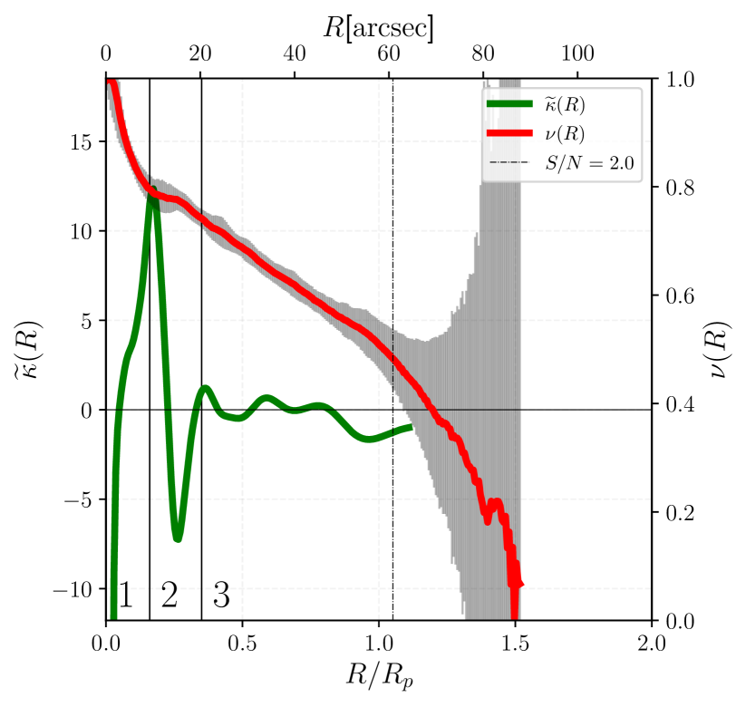
Figure 14: The same as Fig. 4, but for $r$ band of NGC 7723 from Pan-STARRS.

In region 3 (around $R/R_{p}\sim 0.8$) we see a broad and smooth valley of negative curvature, and subsequently being close to zero for $R/R_{p}>1.0$ – this pattern appears because the disk is of type II (Erwin et al., 2008; Muñoz-Mateos et al., 2013) which explains the broad valley, since it comprises larger extension in radius. It is possible to discriminate a valley in $\widetilde{\kappa}$ entailed by the disk of Type II morphology and one related to a ring or a bar. Valleys for bars and rings have high negative gradient in $\widetilde{\kappa}$ and are thin in width (see additional examples in Figs.4, 5, 8, 9, 12, 13 and 14).

For completeness on the analysis of NGC 936, Fig. 6 shows each fundamental region of the profile represented in terms of shaded ellipses, gathered from the behaviour of the curvature. See labels in the plot. Also, the smooth grey circles shows a practical example of Fig. 1 for different osculating circles drawn in the galaxy profile.

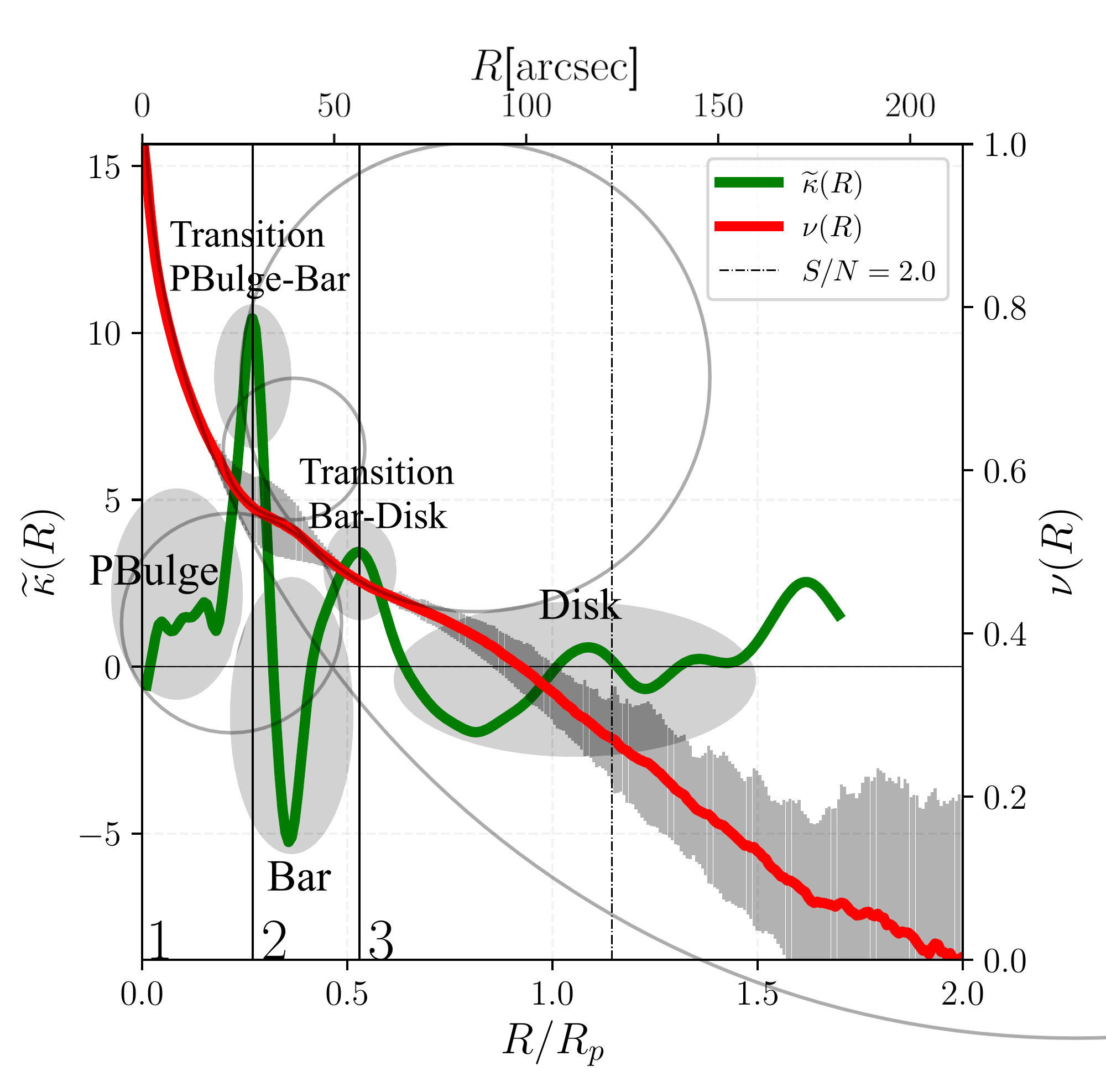
Figure 6: Extra representation of the curvature measured on NGC 936. The shaded ellipses indicates, according to the curvature behaviour, each fundamental region of the profile (see the labels). The four smooth grey circles represents the osculating circles, as in Fig. 1, in some regions of the profile.

NGC 2767

NGC 2767 is classified as an elliptical (de Vaucouleurs et al., 1991) and as a S0 (Nair & Abraham, 2010). However, the structure of this galaxy is not trivial to be resolved. Yıldırım et al. (2017) comment that the PA twist in the centre of the galaxy may imply the existence of a bar and a dust disk. Examining $\widetilde{\kappa}$ in Fig. 9 shows the existence of two peaks and a narrow deep valley, revealing that the galaxy has at least three components (regions 1, 2 and 3). The bulged central part is demarcated by 1. The valley in 2 ($R/R_{p}\sim 0.4$), even not being negative (but $\sim 0$), is much smaller than the neighbouring peaks in terms of amplitude and also is thin, therefore it points to the bar component. The region 3 seems to be of a disk structure of type II, very similar to NGC 936 (note that after $R/R_{p}\sim 1.0$, the curvature is very small). A final note is that, photometrically, we suggest that the bulge of this galaxy is indicated to be pseudobulge due to the behaviour of $\widetilde{\kappa}$ in the inner part of the profile – it takes some distance from the centre to increase significantly until the transition region at $R/R_{p}\sim 0.4$.

Summarizing, in agreement with Yıldırım et al. (2017), the curvature entail that the galaxy may have a bulge+bar+disk structure. The residual image in the middle panel of Fig. 9 demonstrates these structures well within the delimited regions gathered from the curvature in the bottom plot.

NGC 4267

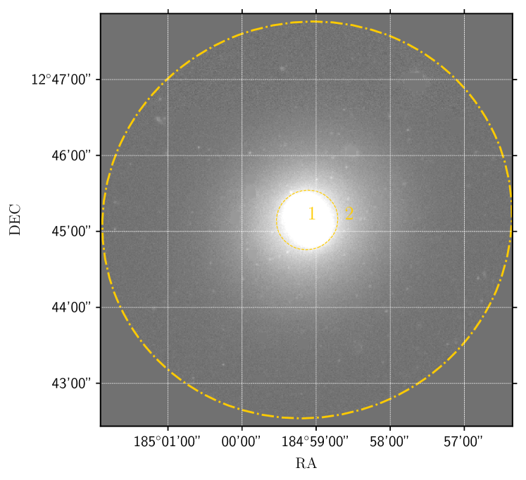
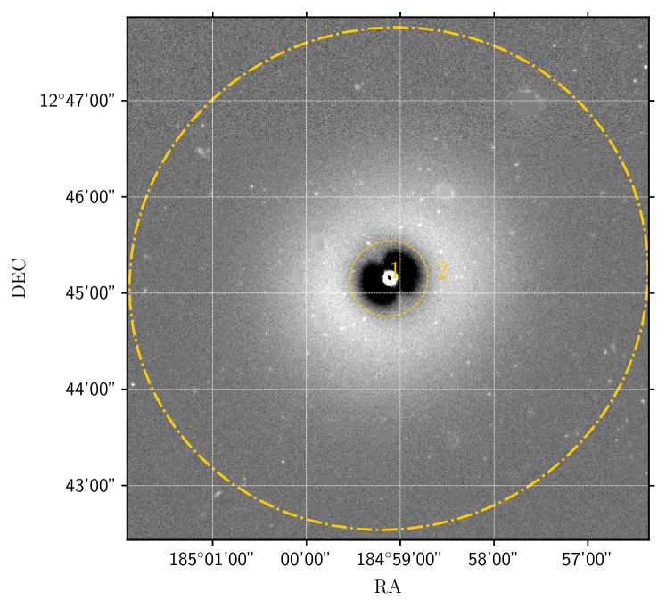
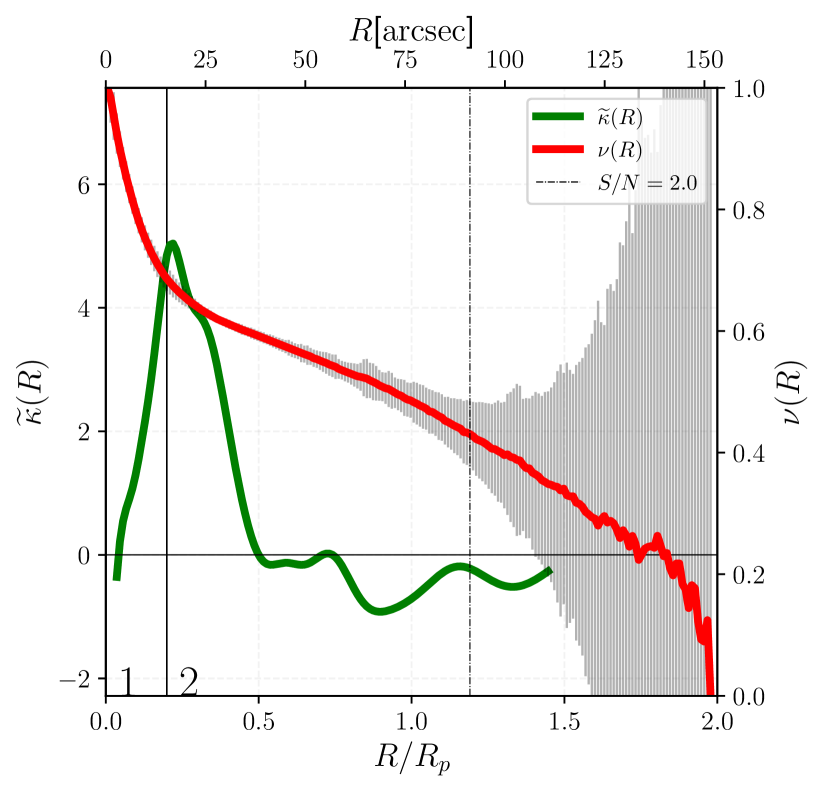
Figure 10: The same as Fig. 4, but for $r$ band of NGC 4267 from EFIGI.

In earlier catalogues (Nilson, 1973) NGC 4267 was classified as S0, but the presence of a bar is also suggested (Sandage & Tammann, 1981; Wozniak & Pierce, 1991; Jungwiert et al., 1997; Gadotti & de Souza, 2006; Erwin et al., 2008) – SB0. The shape of $\widetilde{\kappa}(R)$ is shown in Fig. 10. In comparison to NGC 2767, NGC 4267 exhibit an akin radial profile, however $\widetilde{\kappa}$ is considerably different. Region 1 around $R/R_{p}\sim 0.3$ refers to the bulge while the disk takes part in the remaining of the profile in region 2 (lower $\widetilde{\kappa}$ below zero). In respect to the bar, the curvature does not trace a sign of it because the pattern of a narrow valley is not exhibited. Also combining together the curvature and the residual image (middle panel of Fig. 10), shows no evidence of a photometric bar component. In relation the bulge and the disk, the transition of both is highlighted by the peak in $\widetilde{\kappa}$ at $R/R_{p}\sim 0.3$. The inner region shows an abrupt increase in $\widetilde{\kappa}$ from zero to the transition region with the disk, therefore this points that the bulge is a classical bulge. This is in agreement with (Fisher & Drory, 2010, see their Table 2).

NGC 4417

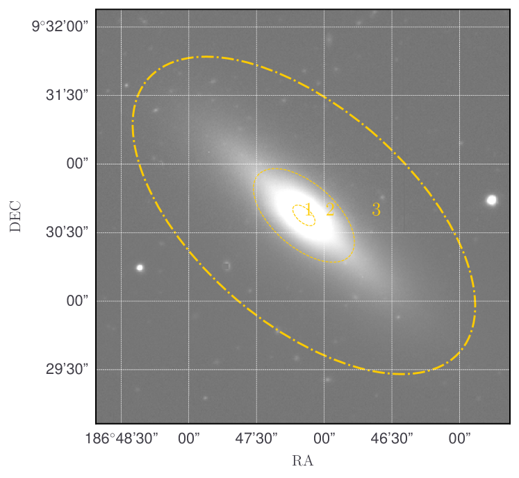
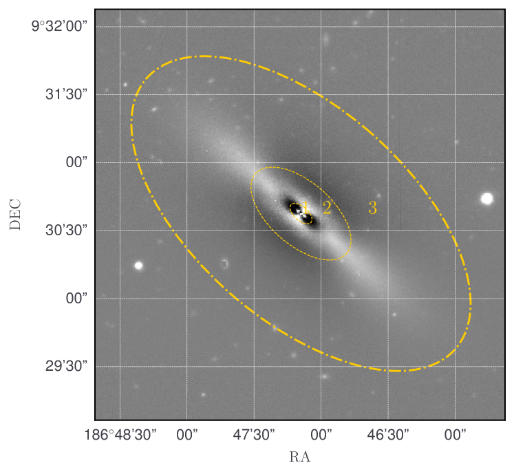
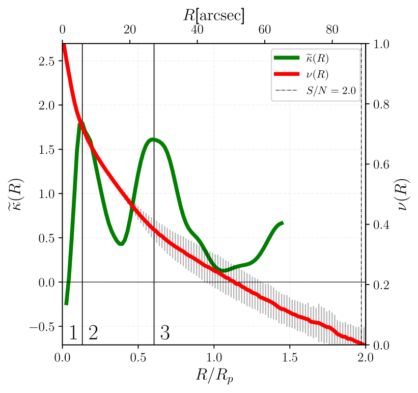
Figure 11: The same as Fig. 4, but for $r$ band of NGC 4417 from EFIGI.

NGC4417 is classified as SB0:edge-on (de Vaucouleurs et al., 1991; Hinz et al., 2003) and also S0:edge-on (Sandage & Tammann, 1981; Nilson, 1973). In the curvature plot of Fig. 11, two peaks stand out in the first half of the $R_{p}$ region: 1 and 2 seems to have a bulge morphology, while 3 is a disk. Analysing $\widetilde{\kappa}$, it seems plausible that it distinguishes two components inside $R/R_{p}\sim 1.0$, the first part identified by the first peak and the second by the second peak. Kormendy & Bender (2012) argued that the inner part (region 1) of this galaxy is an inner disk while the outer region (region 2) is the bulge with a boxy shape due to a faint bar. This seems reasonable because the second component has a small $\widetilde{\kappa}$ in region 2 resembling the behaviour of a bar as in other galaxies. However, in this case we could not differentiate the bulge from the bar. In the residual image it is clear that there are signs of two components, in region 1 a more oval shape while in region 2 a boxy one. Region 3 is related to the edge-on disk, since decreases after $R/R_{p}\sim 1.0$. But, a final note is related to the peak in $\widetilde{\kappa}$ close to $R/R_{p}\sim 1.5$. Due to the signal-to-noise limit and considering that this region is close to the edge of the galaxy, we do not treat it as a transition of components.

5.4 Spirals

NGC1512

NGC 1512 is classified as a barred spiral galaxy SBa (de Vaucouleurs et al., 1991), however there are many references bringing up other components in its morphology: rings, pseudorings, nuclear ring and pseudobulge (see for example Laurikainen et al., 2006; Fisher & Drory, 2008). According to Compère et al. (2014), who conducted a detailed study on this galaxy, it has a bulge, a bar and a disk. Fig. 12 shows the results for $\widetilde{\kappa}$. The region inside $R/R_{p}<0.5$ shows two components delimited by the local peak at $R/R_{p}\sim 0.15$, and both shows small $\widetilde{\kappa}$ compared with the overall curvature profile. From (Laurikainen et al., 2006; Compère et al., 2014), the innermost region (1) is a nuclear ring and region 2 is dominated by the bulge. By the shape of $\widetilde{\kappa}$ one must consider a pseudobulge component, which is in agreement with (Fisher et al., 2009; Fisher & Drory, 2010).

Regarding the bar, it seems that pseudobulge and bar coexist (the change in the position angle and ellipticity between the bulge and the bar is very smooth (see figure 4 of Jungwiert et al., 1997)), with the bar connecting the pseudobulge and the outer ring – according to Fisher & Drory (2008), a pseudoring (region 3). With this configuration, the distinction of the bar and the pseudobulge with $\widetilde{\kappa}(R)$ is not clear, since region 2 encloses both components. Fisher & Drory (2008) also did not fit a bar component separately to NGC 1512 and considered only a Sérsic+Exp fit to it. What is noticeably is the outer ring, the peak at $R/R_{p}\sim 0.5$ points to the transition between the pseudobulge+bar with this ring, which is dominant in region 3. The last smooth peak at $R/R_{p}\sim 1.1$ binds the dominance of the outer ring with a faint disk ($\widetilde{\kappa}$ approaches to zero).

NGC 2273

NGC 2273 is classified as SBa (Nilson, 1973) and SB(r)a (de Vaucouleurs et al., 1991). In Fig. 13 the curvature indicates a small bulge contained inside $R/R_{p}\sim 0.1$ (region 1). Considering the valley in region 2, it retain a gradient in $\widetilde{\kappa}$, considerable lower compared to the first and second local peaks, suggesting a bar component. However this behaviour is not well pronounced here, but still indicates correctly the existence of different structural components. The next valley in region 3 is formed by two tightly wound spiral arms (Laurikainen & Salo, 2017), which behaves like a ring. The fourth peak at $R/R_{p}\sim 0.5$ makes the transition of this component with the outermost region of the galaxy.

Cabrera-Lavers & Garzón (2004) worked on the details considering the aforementioned structures, adding a lens component and assuming that the outer region is a disk. Also, they argue that the bulge is prominent, nevertheless $\widetilde{\kappa}$ indicates that the bulge is not too prominent. This can be evidenced by the fact that the inner region can be formed by other components: Moiseev et al. (2004) noted that the bar is of large scale; Erwin & Sparke (2003); Moiseev et al. (2004) also assert that the innermost region can be built by a nuclear spiral while Mulchaey et al. (1997) says that it is a secondary bar. Also, Erwin & Sparke (2003) says that this galaxy is four-ringed, two of them outer rings (outer region). And additionally, NGC 2273 is also characterized with a barlens component by Laurikainen & Salo (2017).

The curvature give a picture of these rings in region 4 due to small perturbations. In summary we find that $\widetilde{\kappa}$ gives and acceptable constrain that NGC 2273 has a bulge+bar/ring+disk structure.

NGC 7723

NGC 7723 is classified as SB(r)b/SB(rs) (de Vaucouleurs et al., 1991; Comerón, 2013). Fig. 14 shows the result of the curvature for NGC 7723. The bulge is contained inside the region 1 delimited by $R/R_{p}\sim 0.2$. Eskridge et al. (2002) argue that the central part of this galaxy is composed by a boxy bulge with a symmetric nucleus embedded in.

Analysing the valley in region 2 together with the residual image we see that it is related to a bar and a ring. However, the bar is much more prominent (Prieto et al., 2001) than the later and it becomes non-trivial to demonstrate the existence of a ring. In fact, this component is considered to be a pseudoring formed by the way the spiral arms emerges from the bar (del Rio & Cepa, 1998; del Río & Cepa, 1999; Prieto et al., 2001; Eskridge et al., 2002). In Aguerri et al. (2000); Prieto et al. (2001) they mentioned the ring structure but in their structural decomposition they have not taken it into account. The spiral arms begin at $R/R_{p}\sim 0.35$ – and manifests in oscillations of $\widetilde{\kappa}$. del Rio & Cepa (1998) made another commentary arguing that there is a disk outside the spiral arms, however due to our confidence limit $S/N=2$ it is not possible to conclude that this disk exists using $\widetilde{\kappa}$. Still a disk feature can be noted between $0.35\lesssim R/R_{p}\lesssim 1.0$ because the mean value of $\widetilde{\kappa}$ is very low.

NGC 6056

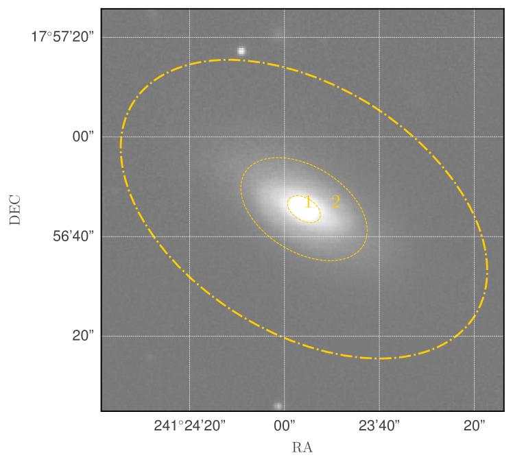
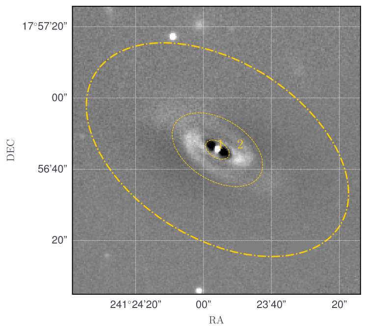
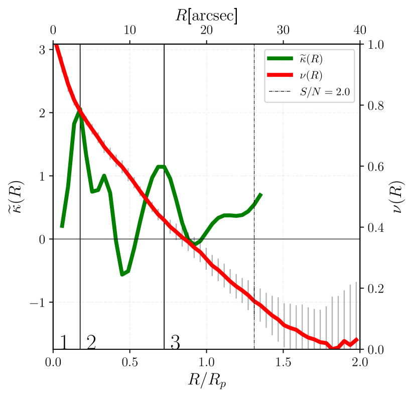
Figure 15: The same as Fig. 4, but for $r$ band of NGC 6056.

This galaxy is considered to be an barred spiral with an internal bulge (SB(s)0) (de Vaucouleurs et al., 1991; Prieto et al., 2001), and also non-barred (S0/a) (Tarenghi et al., 1994). In $\widetilde{\kappa}$ of Fig. 15, the bulge is within $R/R_{p}\lesssim 0.18$ (first peak). The valley in 2 is the bar (the same behaviour in $\widetilde{\kappa}$ as the other galaxies), and confirmed by Prieto et al. (2001). The transition of the bar with the outer disk (spiral) is indicated by the local peak at $R/R_{p}\sim 0.6$.

A pseudobulge component was pointed by Prieto et al. (2001) and they found a Sérsic fit of $n=1.1$ in the $r$ band. But the pseudobulge part does not shows the same behaviour in $\widetilde{\kappa}(R)$ as the other galaxies. This may be attributed to the low resolution of the galaxy image – note that there are few data points in the region related to the bulge.

5.5 Spheroidal components

Unlike spiral and lenticular galaxies, whose components are structurally very diverse (bulge, bar, spiral arms and disk, for example), in the case of spheroidal galaxies (the various kind of ellipticals, bulges and some lenticular) the differences in the components are much more subtle. Consider, for instance, that many elliptical galaxies substructures cannot be seen in raw images, but rather, reveal themselves after image manipulation techniques, such as unsharp masking, brightness profile modelling and so on. In this way, we may regard that the effects that the different component of elliptical galaxies have on the curvature are more faint than for spiral galaxies.

NGC 1270

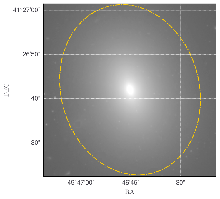
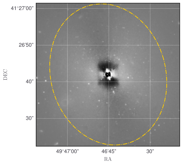
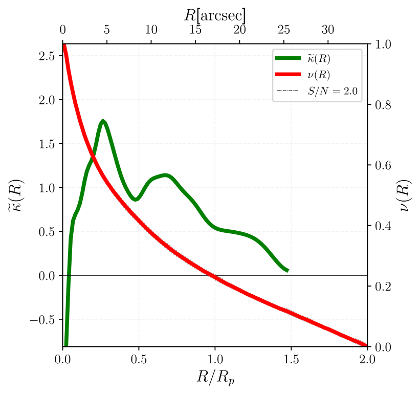
Figure 16: The same as Fig. 4, but for NGC 1270 from HST (f160w).

NGC 1270 is classified as an elliptical galaxy (de Vaucouleurs et al., 1991) and further as a compact elliptical galaxy (Yıldırım et al., 2017). The curvature $\widetilde{\kappa}(R)$ is displayed in Fig. 16, its shape is not continuous (as expected) and having small oscillations of low scale. However, the curvature has a smooth overall shape, is high in inner regions (around $R/R_{p}\sim 0.2$) and drops to near zero at large radius. As can be seen in the residual image, the central region ($R/R_{p}\lesssim 0.20$) indicates an inner spheroidal component with different properties compared to the main body of the galaxy (missing light regarding the model for the main body). There is a sign of a small disk within $R/R_{p}\lesssim 0.1$ aligned with the apparent main axis of the galaxy.

NGC 472

NGC 472 is a compact elliptical galaxy (Yıldırım et al., 2017). Similar to NGC 1270, it does show some perturbations in the inner regions – the two local peaks are attributed to inhomogeneities – but the shape of $\widetilde{\kappa}$ follows an overall shape resembling a pure component, which is smooth and decreases from inner to outer regions. The great difference between NGC 472 and NGC 1270 is that for NGC 1270 the increasing of $\widetilde{\kappa}$ in the innermost part is more subtle than NGC 472. Lastly, a single Sérsic fit $n=5.8$ returned a robust representative model for NGC 472, since there is no residual structures in the outer regions.

NGC 384

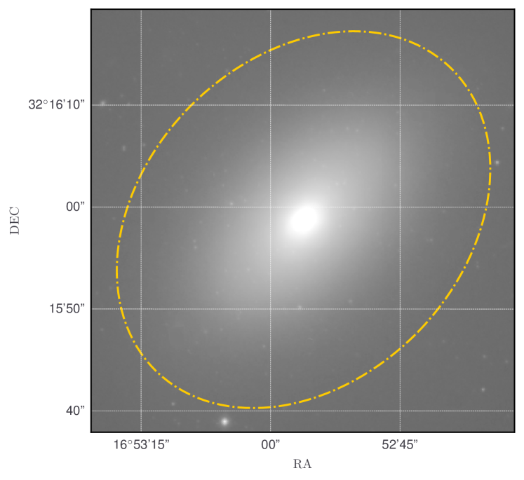
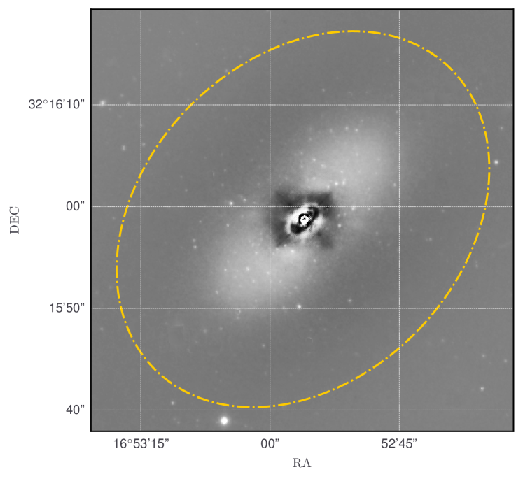
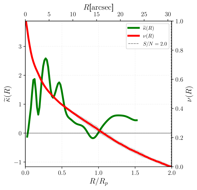
Figure 18: The same as Fig. 4, but for NGC 384 from HST (f160w).

NGC 384 is classified in literature as E (de Vaucouleurs et al., 1991; Yıldırım et al., 2017) but also S0 (Nilson, 1973). In comparison to NGC 472 and NGC 1270, $\widetilde{\kappa}(R)$ is quite different (Fig. 18) due to the emergence of the substantial oscillations in the region $R/R_{p}\lesssim 0.5$. These delineates some internal and small structure. In the residual image of Fig. 18 it is readily seem such structure with a disk oval shape.

NGC 1052

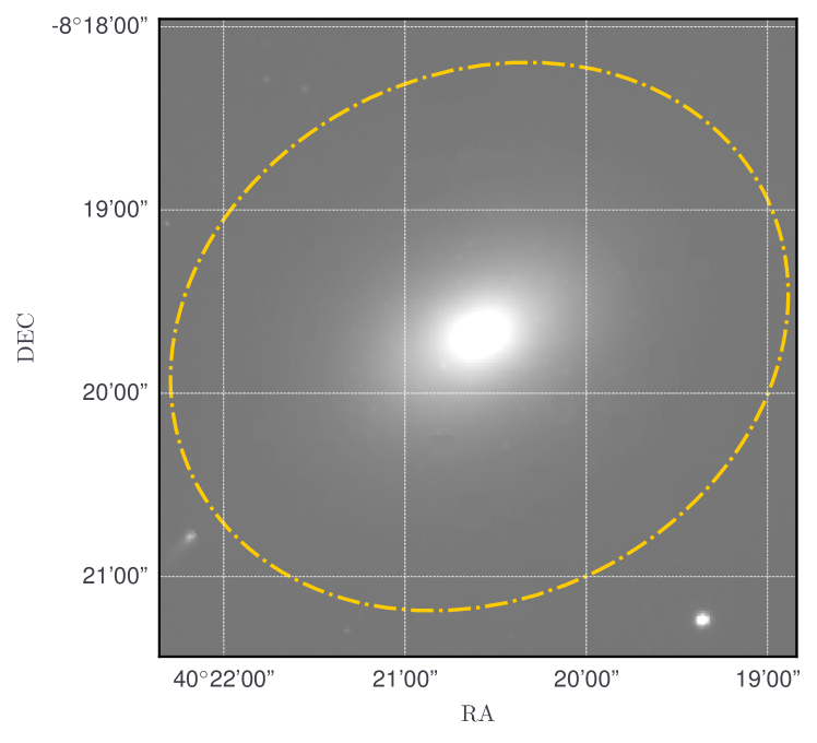
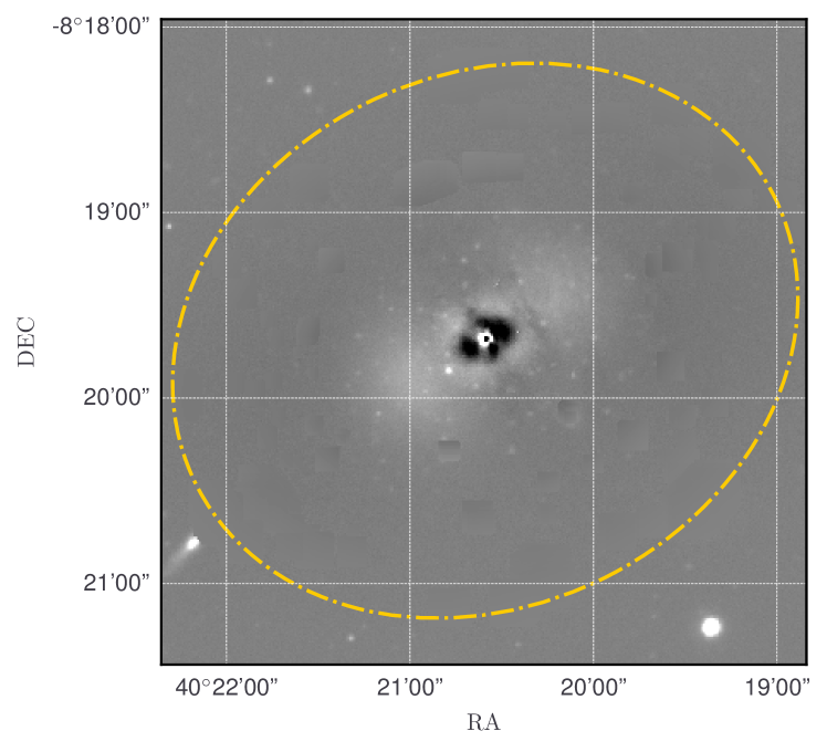
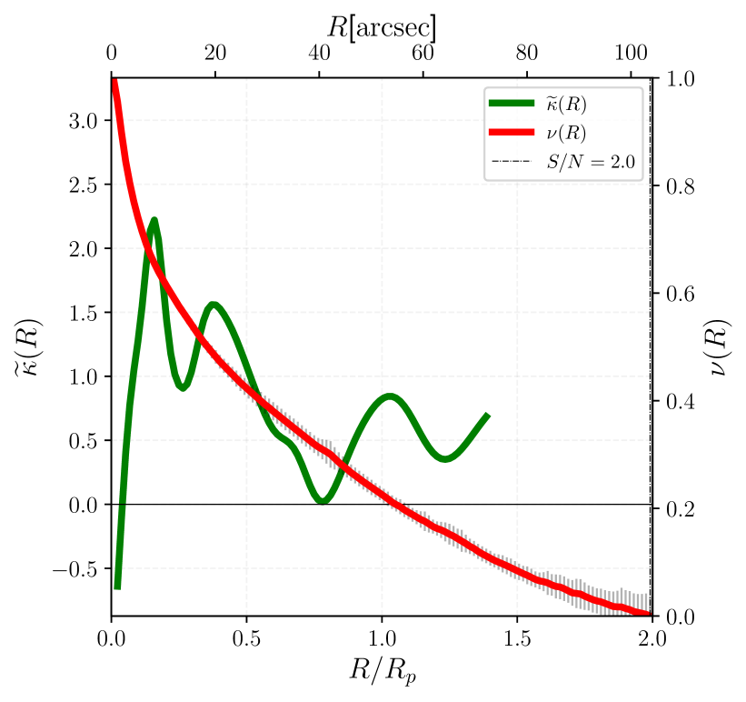
Figure 19: The same as Fig. 4, but for $r$-band of NGC 1052 from EFIGI.

NGC1052 is classified as an elliptical galaxy (de Vaucouleurs et al., 1991) and as E/S0 (Sandage & Tammann, 1981). Lauer et al. (2007) indicates the presence of a core. In Fig. 19 the curvature suggests some possible transition around $R/R_{p}\sim 0.15$, in which, therefore, might be between the core structure and the remaining structure of an elliptical. Furthermore, (Milone et al., 2007, and references therein) conclude that NGC 1052 has a rotating disk. The curvature may indicate such kind of component because the mean small values after $R/R_{p}\sim 0.6$, however such disk seems not to be exponential. The disk is also seen in the residual image.

6 Discussion

Galaxy structural analysis has been traditionally tackled with parametric methods of model fitting. Currently, given the amount of data available, there is a growing need of using non-parametric methods that do not have an underlying model and that require less user intervention. The curvature, being non-parametrical, can provide us with a framework that allow us to automate the galaxy structural analysis and thus its appliance to large datasets.

With our set of 14 galaxies, distinct behaviours appeared to relate to the curvature. The basics is that regions dominated by different structural components have its own shape in the surface brightness and we can use $\widetilde{\kappa}$ to unveil the difference between each one. The curvature is sensitive to smooth (e.g NGC 384, NGC 6056) or abrupt variations (e.g. NGC 1512, NGC 7723) of the light profile. High concentrated regions have high values of $\widetilde{\kappa}$ (in relation to the overall of each curvature profile), but transitions regions also reveal high $\widetilde{\kappa}$. This happens because along the radius, a transition is a smooth discontinuity of the inner part, which gives rise to the next component – i.e. the point where the profile changes from one component to another – and frequently has a different slope (higher) than the slope characteristic of each profile alone.

Below we discuss the signature of each component in the curvature profile related to the individual galaxies. At this stage of the technique, there is no clear discrimination between bars and rings from the 1D curvature profile. For these cases there may be a limit of the method when signatures of bulges, bars, and rings overlap in the 1D profile. We will explore this and other issues in a forthcoming paper.

Bars

Bars and rings show a depression pattern in $\widetilde{\kappa}$ where these components dominates. For NGC 936 (Fig. 8), NGC 2767 (Fig. 9) and NGC 7723 (Fig. 14) the bars have a distinct valley between the two local peaks, region $2$ of each galaxy. These bars are represented by the narrows valleys in $\widetilde{\kappa}$ (note the difference between a narrow valley in $\widetilde{\kappa}$ related to a bar and a broad valley related to a disk type II in region 3 of NCG 936). For the faint bar of NGC 2273 (Fig. 13), the curvature exhibit a deep but non-negative valley in region 2 (between the two local peaks), and the same applies to NGC 6056 (Fig. 15). We found that the depression in $\widetilde{\kappa}$ for bars is not always negative , but considerably lower than the local peaks. For NGC 1512 (Fig. 12) the curvature does not indicate well the bar in region 2 because bulge and bar appear to show a subtle transition.

Rings

Galaxies NGC 1512 (Fig. 12), NGC 2273 (Fig. 13) and NGC 7723 (Fig. 14) have rings. They exhibit a high and narrow negative gradient in region 3 (first two) and region 2 (last one). These ring structures are also likely to be formed by the tight morphology of the spiral arms after the end of the bar, for example NGC 2273 and NGC 7723. One issue in 1D curvature profile at the current stage is that it may not be possible unravel the differences between bars and rings.

Disks and spiral arms

The most notable galactic disk absent of spiral arms that shows values of $\widetilde{\kappa}$ close to zero is that of NGC 4267 (Fig. 10). For NGC 936 (Fig. 8) the disk is of Type II, therefore it shows a broad valley in region 3 (a kind of transition between inner and outer parts of type-II disks). In the outer part of the disk, the curvature approaches zero. A similar result is found for NGC 2767 (Fig. 9). Another case is NGC 4417 (Fig. 11) which in region 3 shows a decreasing $\widetilde{\kappa}$ and reach small values, regarding that not all galaxy disks follows a $n=1$ Sérsic law, therefore there are disk components that exhibit $\widetilde{\kappa}>0$ or $\widetilde{\kappa}<0$.

NGC 1357 (Fig. 5), NGC 2273 (Fig. 13), NGC 7723 (Fig. 14) and NGC 6056 (Fig. 15) have spiral arms. For NGC 7723 the spirals arm are well identified by $\widetilde{\kappa}$ at the inner to middle part of region 3, due to the homogeneous oscillations. Galaxy NGC 1357 also shows two oscillations of this kind from the middle onwards part of region 3. For NGC 2273, the pattern in $\widetilde{\kappa}$ is not well defined, but we still get an indication of a perturbed disk in region 4. The spiral galaxy in which the spiral structure does not appear clearly is NGC 6056.

Spheroidal

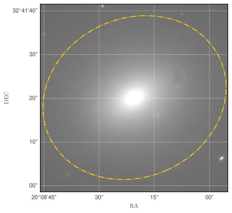
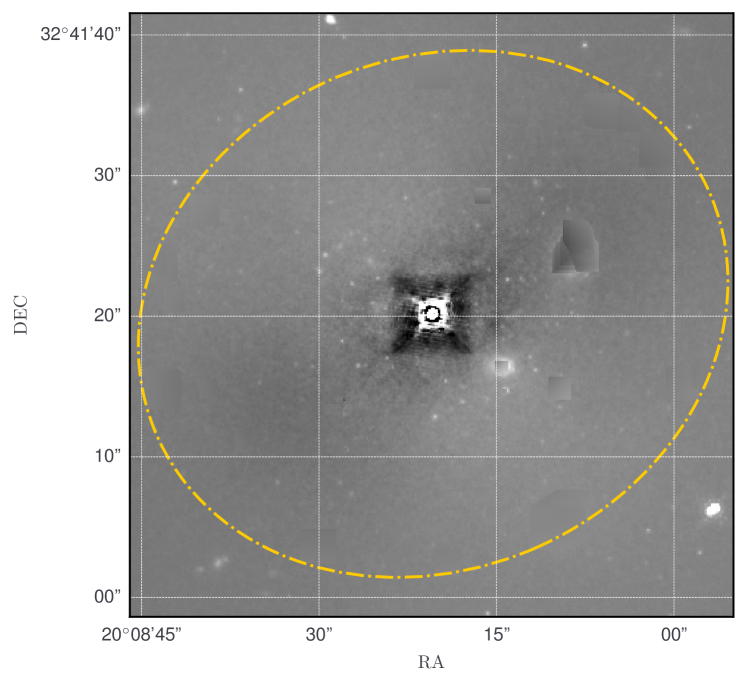
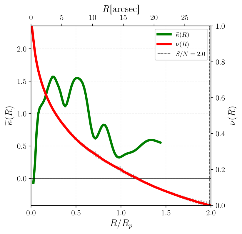
Figure 17: The same as Fig. 4, but for NGC 472 from HST (f160w).

For our elliptical galaxies the curvature behaviour also revealed interesting results. For NGC 384 (Fig. 18) $\widetilde{\kappa}$ revealed an inner component due to the perturbations in region $R/R_{p}<0.5$, which is a inner dust disk. For NGC 472 (Fig. 17), NGC 1052 (Fig. 19) and NGC 1270 (Fig. 16) $\widetilde{\kappa}$ also indicates perturbations of $I(R)$. This behaviour indicates that these galaxies are not a complete homogeneous system but are formed by heterogeneous light distribution. This means that even in systems with subtle variations of the brightness profile, we can unveil the existence of perturbations in the galaxy’s structure.

Pseudobulges

Another important result we found on this work is the behaviour of $\widetilde{\kappa}$ for pseudobulges. Inner regions that shows small values of curvature compared to the values of posterior regions, and a subtle increasing in the values, might infer pseudobulge components. In our sample the cases are NGC 1211 (Fig. 4), NGC 936 (Fig. 8), NGC 2767 (Fig. 9), NGC 1512 (Fig. 12), NGC 2273 (Fig. 13) and NGC 7723 (Fig. 14) but for NGC 2273 and NGC 7723 this pattern is not too clear. For NGC 2767 there is no reference in literature indicating that the bulge is pseudo.

In summary, pseudobulges curvatures display a distinct pattern. Since pseudobulges are in some cases similar to disks – having surface brightness profiles similar to exponentials – the curvature might in general shows a behaviour that resembles a disk, we mean this by having small values in inner regions and no abrupt variations (fast increasing) in some range of $R$.

7 Summary

We summarise bellow our conclusions in using the curvature of the brightness profile for structural analysis. We have introduced the curvature of the brightness profile of galaxies as a tool to identify and study their different structural components, most notably bulges, bars, discs, rings and spiral arms. The underlying argument for such is that these components have distinct Sérsic index (or concentration) which directly impact the curvature. But, unlike standard multicomponent modelling of light profiles, the curvature is non parametric and does not depend on model parameters.

We measured the curvature profile for structural analysis in 14 galaxies (Tab. 1) comprising different morphologies. For these galaxies, we identified their structural components and inferred their domain regions in terms of the local peaks in $\widetilde{\kappa}(R)$; following the peaks in the measured curvature profile we spotted the matching regions in the image and residual maps where the different components can be identified and related to the curvature behaviour. Thus regarding the curvature curve (in terms of logarithm normalized scale of intensity): 1. pseudobulges have small values (compared to the highest absolute values) or near zero curvature in their regions; 2. Bars and rings have similar narrow valleys in $\widetilde{\kappa}$ (negative or small values) although they are inextricable regarding the profile; 3. Disks have a broad profile in the curvature with near zero (Type I) or negative (Type II) values. 4. the curvature in elliptical galaxies shows that they also are not completely homogeneous systems.

Appendix A Curvature for a Sérsic profile

A good description of brightness profile of different components of galaxies is given by the Sérsic law (Sérsic, 1963, 1968; Ciotti & Bertin, 1999)

$$I(R)=I_{n}\exp\left\{-b_{n}\left[\left(\frac{R}{R_{n}}\right)^{1/n}-1\right]\right\}$$ (12)

where $R_{n}$ (effective radius) is the radii that contain half of the total luminosity of the galaxy integrated to infinity $L(R=R_{n})=0.5L_{T}^{\infty}$, and $I_{n}$ is the effective surface brightness, i.e. the value of $I(R)$ at $R=R_{n}$, and $n$ controls the concentration of the profile. The term $b_{n}$ is defined to make the above definitions hold (Ciotti & Bertin, 1999)

$$b_{n}=2n-\frac{1}{3}+\frac{4}{405n^{2}}+\frac{46}{25515n^{2}}.$$ (13)

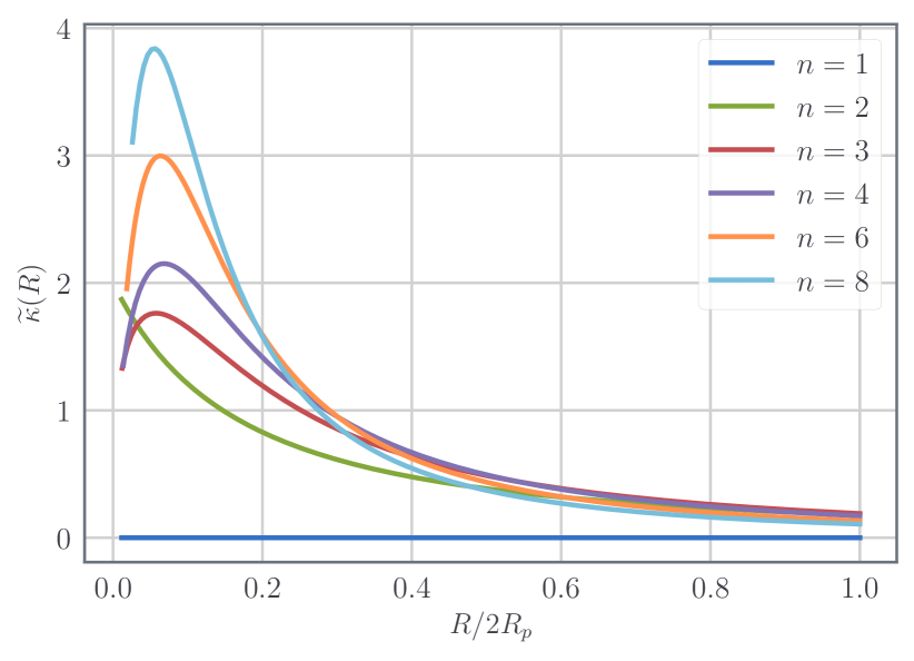
Figure 7: Plots of Equation (20) for different Sérsic indexes. The higher is $n$, the higher is $\widetilde{\kappa}$ in the inner regions. Note that for large $R$, the $\widetilde{\kappa}$ profiles are similar, which is reasonable because high $n$ represent more changes in inner part of the profile.

Here we derive the curvature of a Sérscic law for a single component. As commented, to remove the scale on $I$, we use normalization given by (3). Taking the logarithm of equation (12) we have

$$\nu(R)\equiv\log I(R)=\log I_{n}+b(n)\left[1-\left(\frac{R}{R_{n}}\right)^{1/n}\right].$$ (14)

Since we consider galaxies extending up to $2R_{p}$, the maximum and minimum are at $R=0$ and $R=2R_{p}$, respectively, hence

$$\max\log I=I(0)=\log I_{n}+b(n)$$ (15)

$$\min\log I=I(2R_{p})=\log I_{n}+b_{n}\left[1-\left(\frac{2R_{p}}{R_{n}}\right)^{1/n}\right]$$ (16)

thus, inserting these into (3) gives

$$\nu(R)=1-\left(\frac{R}{2R_{p}}\right)^{1/n}.$$ (17)

This result is independent of $I_{n}$ and $R_{n}$ because of the normalization on $I$ and $R$. The first and second derivative are

$$\frac{\text{d}\nu(R)}{\text{d}R} =-\frac{1}{2R_{p}n}\left(\frac{R}{2R_{p}}\right)^{\frac{1-n}{n}}$$ (18)

$$\frac{\text{d}^{2}\nu(R)}{\text{d}R^{2}} =\frac{n-1}{4R_{p}^{2}n^{2}}\left(\frac{R}{2R_{p}}\right)^{\frac{1-2n}{n}}.$$ (19)

Using these two result in equation (9) we obtain the normalized curvature for a single Sérsic profile:

$$\widetilde{\kappa}(R)=\frac{\frac{n-1}{n^{2}}\left(\frac{R}{2R_{p}}\right)^{\frac{1-2n}{n}}}{\left[1+\frac{1}{n^{2}}\left(\frac{R}{2R_{p}}\right)^{\frac{2-2n}{n}}\right]^{3/2}}$$ (20)

Fig. 7 shows plots of (20) for different values of $n$ against the normalized variable $\chi=R/(2R_{p})$. For a disk, which frequently follows a $n\sim 1$ law, we obtain that $\widetilde{\kappa}\sim 0$ because the numerator vanishes. For $n>1$, $\widetilde{\kappa}$ is correlated to $n$, the higher the $n$ the higher the curvature (in inner regions), for outer regions the Sérsic law becomes more flat and $\widetilde{\kappa}$ behaves a disk.

Appendix B Additional Curvature Plots

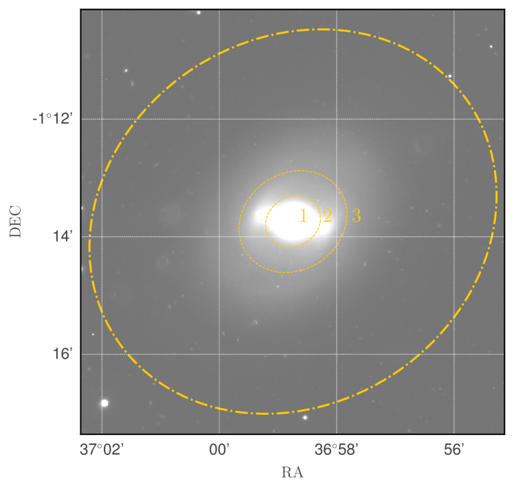
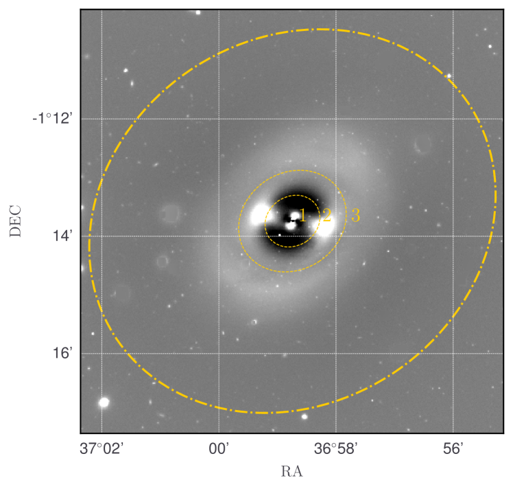
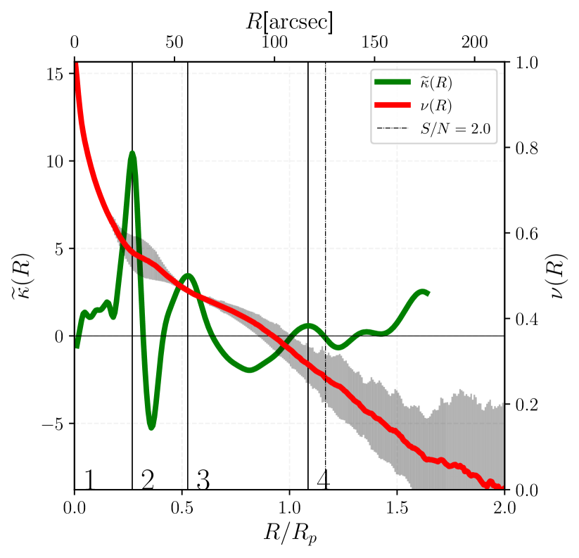
Figure 8: The same as Fig. 4, but for $r$ band of NGC 936 from EFIGI. See text for details.

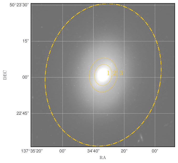
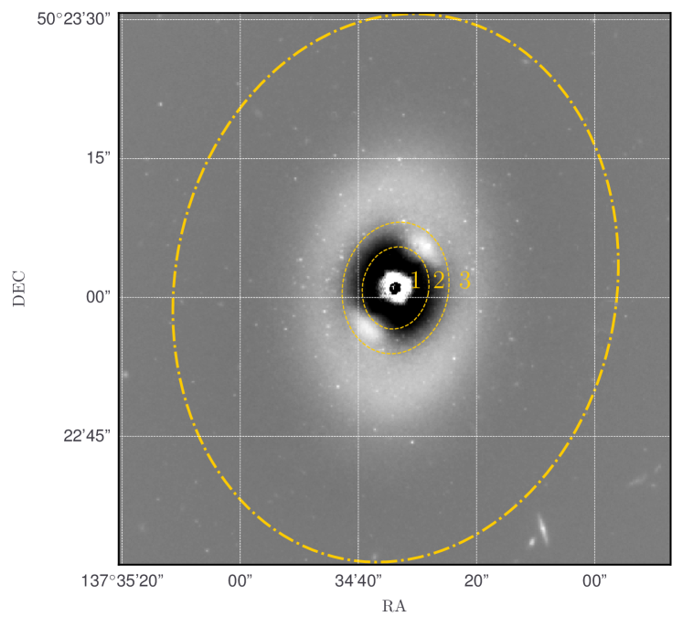
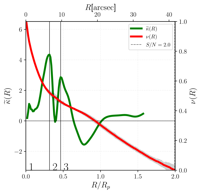
Figure 9: The same as Fig. 4, but for NGC 2767 from HST (f160w).

References

- Abazajian et al. (2003) Abazajian K., et al., 2003, The Astronomical Journal, 126, 2081
- Aguerri et al. (2000) Aguerri J. A. L., Varela A. M., Prieto M., Muñoz- Tuñón C., 2000, The Astronomical Journal, 119, 1638
- Andrae et al. (2011) Andrae R., Jahnke K., Melchior P., 2011, Monthly Notices of the Royal Astronomical Society, 411, 385
- Argyle et al. (2018) Argyle J. J., Méndez-Abreu J., Wild V., Mortlock D. J., 2018, preprint, (arXiv:1807.02097)
- Ascasibar & Gottlöber (2008) Ascasibar Y., Gottlöber S., 2008, Monthly Notices of the Royal Astronomical Society, 386, 2022
- Athanassoula (2005) Athanassoula E., 2005, Monthly Notices of the Royal Astronomical Society, 358, 1477
- Baillard et al. (2011) Baillard A., et al., 2011, A&A, 532, A74
- Bershady et al. (2000) Bershady M. A., Jangren A., Conselice C. J., 2000, The Astronomical Journal, 119, 2645
- Binney (2013) Binney J., 2013, Dynamics of secular evolution. p. 259
- Blanton et al. (2001) Blanton M. R., et al., 2001, The Astronomical Journal, 121, 2358
- Bruce et al. (2014) Bruce V. A., et al., 2014, Monthly Notices of the Royal Astronomical Society, 444, 1660
- Burkert & Naab (2003) Burkert A., Naab T., 2003, Major Mergers and the Origin of Elliptical Galaxies. Springer Berlin Heidelberg, Berlin, Heidelberg, pp 327–339, doi:10.1007/978-3-540-45040-5˙27, https://doi.org/10.1007/978-3-540-45040-5_27
- Buta (2013) Buta R. J., 2013, Galaxy Morphology. p. 155