H${}_{3}^{+}$ as a five-body problem described with explicitly correlated Gaussian basis sets

Abstract

Various explicitly correlated Gaussian (ECG) basis sets are considered for the solution of the molecular Schrödinger equation with particular attention to the simplest polyatomic system, H${}_{3}^{+}$. Shortcomings and advantages are discussed for plain ECGs, ECGs with the global vector representation, floating ECGs and their numerical projection, and ECGs with complex parameters. The discussion is accompanied with particle density plots to visualize the observations. In order to be able to use large complex ECG basis sets in molecular calculations, a numerically stable algorithm is developed, the efficiency of which is demonstrated for the lowest rotationally and vibrationally excited states of H₂ and H${}_{3}^{+}$.

I Introduction

Recent progress in the experimental energy resolution Cheng et al. (2018); Markus and McCall (2019) of spectroscopic transitions of small molecules urges theoretical and computational methods to deliver orders of magnitude more accurate molecular energies than ever before. The current and near future energy resolution of experiments allow for a direct assessment of relativistic quantum electrodynamics effects and beyond them, as soon as calculations with a low uncertainty become available. For small molecules, composed from just a few electrons and a few nuclei, this endavour should be realistic within the near future. A remarkable experiment–theory concourse has been unfolding for the three-particle H${}_{2}^{+}$ molecular ion Korobov et al. (2017); Alighanbari et al. (2018) and for the four-particle H₂ molecule Cheng et al. (2018); Wang and Yan (2018); Puchalski et al. (2019); Hölsch et al. (2019). In addition, there are promising initial results for the five-particle He${}_{2}^{+}$ Tung et al. (2012); Semeria et al. (2016); Mátyus (2018); Jansen et al. (2018) for which an explicit five-particle treatment, at least for the lowest vibrational and rotational excitations, should be possible Stanke et al. (2009).

H${}_{3}^{+}$ is also a five-particle system, but it is a polyatomic system. In comparison with atoms and diatomic molecules, there has been very little progress achieved for polyatomics over the past two decades regarding an accurate description of the coupled quantum mechanical motion of the electrons and the atomic nuclei. In addition to the variational treatment considered in the present work, non-adiabatic perturbation theory offers an alternative route for closing the gap between theory and experiment. The single-state non-adiabatic Hamiltonian has been know for a long time Herman and Asgharian (1966); Herman and Ogilvie (1998); Bunker and Moss (1977, 1980); Pachucki and Komasa (2009); Scherrer et al. (2017) and has been used a few times in practice Schwenke (2001); Przybytek et al. (2017); Mátyus (2018), while the general working equations for the effective non-adiabatic nuclear Hamiltonian for multiple, coupled electronic states have been formulated only recently Mátyus and Teufel (2019).

We have already worked on the development of explicitly correlated Gaussian (ECG) ansätze in relation with the variational solution of polyatomics (electrons plus nuclei). Last year, we proposed to use (numerically) projected floating ECGs, which allowed us to approach the best estimate obtained on a potential energy surface (PES) for the Pauli-allowed ground state within 70 cm^-1 (31 cm^-1 with basis set extrapolation) Muolo et al. (2018a).

The present work starts with an overview of the advantages and shortcomings of the different ECG representations together with proton density plots which highlight important qualitative features. Then, we develop an algorithm which ensures a numerically stable variational optimization of extensive sets of ECGs with complex parameters, another promising ansatz for molecular calculations Bubin and Adamowicz (2006, 2008), and demonstrate its applicability for the lowest rotational and vibrational states of H₂ and H${}_{3}^{+}$.

II Explicitly correlated Gaussians

We consider the solution of the time-independent Schrödinger equation (in Hartree atomic units) including all electrons and atomic nuclei, in total $N_{\text{p}}$ particles, of the molecule,

$$\left[-\sum_{i=1}^{N_{\text{p}}}\frac{1}{2m_{i}}\Delta_{\boldsymbol{r}_{i}}+\sum_{i=1}^{N_{\text{p}}}\sum_{j>i}^{N_{\text{p}}}\frac{Z_{i}Z_{j}}{|\boldsymbol{r}_{i}-\boldsymbol{r}_{j}|}\right]\Psi=E\Psi\;.$$ (1)

with electric charges $Z_{i}$, $Z_{j}$ and positions $\boldsymbol{r}_{i}$, $\boldsymbol{r}_{j}$. The exact quantum numbers of the molecular energies and wave functions, $E$ and $\Psi$, are the total angular momentum quantum numbers, $N$ and $M_{N}$, the parity, $p$, and the spin quantum numbers for each particle type, $S_{a},M_{S_{a}},S_{b},M_{S_{b}},\ldots$.

We obtain increasingly accurate approximations to the $\Psi$ molecular wave function by using a linear combination of anti-symmetrized products of (many-particle) spatial, $\psi_{i}^{[N,M_{N},p,]}$, and spin, $\chi_{i}^{[S_{a},M_{S_{a}},S_{b},M_{S_{b}},\ldots]}$, functions,

$$\Psi^{[N,M_{N},p,S_{a},M_{S_{a}},S_{b},M_{S_{b}},\ldots]}=\sum_{i=1}^{N_{\text{b}}}c_{i}\hat{\mathcal{A}}\{\psi_{i}^{[N,M_{N},p]}\chi_{i}^{[S_{a},M_{S_{a}},S_{b},M_{S_{b}},\ldots]}\}\;,$$ (2)

where $N_{\text{b}}$ is the number of basis functions and $\hat{\mathcal{A}}$ is the anti-symmetrization operator for fermions (we would need to symmetrize the product for bosonic particles). The non-linear parameters of the spatial and the spin functions are optimized based on the variational principle Suzuki and Varga (1998); Mitroy et al. (2013) and the $c_{i}$ coefficients are determined by solving the linear variational problem in a given basis set.

Concerning the construction of the basis set, explicitly correlated Gaussian (ECG) functions have been successfully used as spatial basis functions for a variety of chemical and physical problems Bubin et al. (2013); Mitroy et al. (2013). In what follows, we consider various ECG basis sets aiming at an accurate solution approaching spectroscopic accuracy spe of the molecular Schrödinger equation. A precise description of vibrational states of di- and polyatomic molecules assumes the use of basis functions which have sufficient flexibility to describe the nodes of the wave function along the interparticle distances, sharp peaks corresponding to the localization of the nuclei displaced from the center of mass, and allow us to obtain efficiently the solutions corresponding to the exact quantum numbers of this non-relativistic problem.

Concerning the spin functions, we use the spin functions of two and three identical spin-1/2 fermions (electrons and protons) with the spin quantum numbers $(S,M_{S})=(0,0)$ and $(S,M_{S})=(1/2,1/2)$, respectively, formulated according to Refs. Mátyus and Reiher (2012); Suzuki and Varga (1998).

In the case of H${}_{3}^{+}$, the mathematically lowest-energy (ground electronic, zero-point vibrational) state of the Schrödinger equation with $N=0$ and $p=+1$ is not allowed by the Pauli principle (for the $S_{\text{e}}=0$ electrons’ and $S_{\text{p}}=1/2$ protons’ spin states), or in short, the non-rotating vibrational and electronic ground state of H${}_{3}^{+}$ is spin forbidden Lindsay and McCall (2001); Bunker and Jensen (1998). The lowest-energy, Pauli-allowed state is the vibrational ground state ($v=0$) with $N=1$ and $p=-1$ (the first rotationally excited state). The lowest-energy state with $N=0$ is the $(0,1^{1})$ fundamental vibration Lindsay and McCall (2001), which corresponds to asymmetric distortions (anti symmetric for the proton exchange) with respect to the equilateral triangular equilibrium structure.

For the assessment and visualization of the results obtained with the different spatial basis sets, we use particle density functions, which are very useful in analyzing the qualitative properties of the molecular wave function Mátyus et al. (2011a, b); Schild (2019). We will focus on properties of the proton (p) density (measured from the center-of-mass, CM, position):

$$D_{p,\text{CM}}(\boldsymbol{R})=\langle\Psi|\delta(\boldsymbol{r}_{p}-\boldsymbol{r}_{\text{CM}}-\boldsymbol{R})|\Psi\rangle\;.$$ (3)

II.1 Plain ECG, polynomial ECG, and ECG-GVR

Plain ECG-type functions,

$$\psi_{\text{ECG}}(\boldsymbol{A};\boldsymbol{r})=\exp\left[-\boldsymbol{r}^{\text{T}}(\boldsymbol{A}\otimes I_{3})\boldsymbol{r}\right]\;$$ (4)

with the $\boldsymbol{A}\in\mathbb{R}^{N_{\text{p}}\times N_{\text{p}}}$ symmetric matrix, have been successfully used to describe atoms and positron-electron complexes (with $N=0$ total angular momentum quantum number and $p=+1$ parity) Suzuki and Varga (1998). To describe the localization and vibrational excitation of atomic nuclei, a linear combination of several plain ECG functions is necessary, which makes their use in molecular calculations very inefficient. The slow convergence of plain ECGs for the lowest-energy $N=0$ state of H${}_{3}^{+}$ is shown with respect to ECG-GVR (vide infra) in Figure 1 (compare sub-Figures 1a and 1b).

Explicitly correlated Gaussians with the global vector representation (ECG-GVR) have been originally proposed by Suzuki, Usukura, and Varga in 1998 Suzuki et al. (1998). These functions represent a general form of ECGs with polynomial prefactors. When several ECG-GVR functions are used in a variational procedure, molecular states can be converged with a total angular momentum quantum number, $N$, and natural parity, $p=(-1)^{N}$:

$$\psi^{[N,M_{N}]}_{\text{ECG-GVR}}(\boldsymbol{r};\boldsymbol{A},\boldsymbol{{u}},K) =Y_{NM_{N}}(\hat{\boldsymbol{v}})\ |\boldsymbol{v}|^{2K+N}\ \exp\left[-\boldsymbol{r}^{\text{T}}(\boldsymbol{A}\otimes I_{3})\boldsymbol{r}\right]\;,$$ (5)

where the ‘global vector’ $\boldsymbol{v}$ is a linear combination of particle coordinates,

$$\boldsymbol{v}={u}_{1}\boldsymbol{r}_{1}+{u}_{2}\boldsymbol{r}_{2}+\ldots+{u}_{N_{\text{p}}}\boldsymbol{r}_{N_{\text{p}}}=(\boldsymbol{{u}}\otimes\boldsymbol{I}_{3})^{\text{T}}\boldsymbol{r}\;,$$ (6)

and $\hat{\boldsymbol{v}}$ contains the spherical polar angles corresponding to the unit vector $\boldsymbol{v}/|\boldsymbol{v}|$.

The general ECG-GVR basis set can be very well used to converge the ground- and excited states of atoms, positron-electron complexes, as well as diatomic molecules (for which plain ECGs would be inefficient) with various total angular momentum quantum numbers $N$ Armour et al. (2005); Varga et al. (1998a); Mátyus and Reiher (2012); Mátyus (2013); FeM . It is important to stress, however, that higher vibrational excitations, heavier nuclei, or higher $N$ values require the use of higher-order polynomials in front of the ECG, which make the integral evaluation and the entire calculation computationally more demanding.

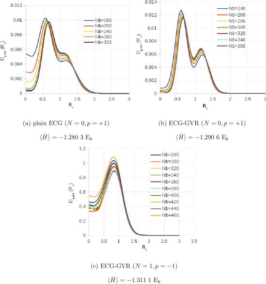
Figure 1: Proton probability density for H${}_{3}^{+}=\{\text{p}^{+},\text{p}^{+},\text{p}^{+},\text{e}^{-},\text{e}^{-}\}$ ($S_{\text{e}}=0$, $S_{\text{p}}=1/2)$ obtained with plain ECG and ECG-GVR functions (the density is shown along a ray measured from the center of mass). In the ECG-GVR calculations the maximal order for the polynomial prefactor was $2K_{\text{max}}=20$. The reference energy values obtained by us on a PES are $E_{\text{PES}}(N=0,p=+1)=-1.311\ 950$ $\text{E}_{\text{h}}$ and $E_{\text{PES}}(N=1,p=-1)=-1.323\ 146$ $\text{E}_{\text{h}}$ pes (note that the latter value corresponds to the lowest-energy Pauli-allowed state). All quantities in the figure are given in atomic units.

For $N=0$, an ECG-GVR with the special parameterization $u_{i}=1$, $u_{j}=-1$ and $u_{k}=0$ $(k\neq i,j)$, simplifies to an ECG with a single (even-power) polynomial prefactor,

$$\psi^{[0,0]}_{\text{ECG-r}}(\boldsymbol{r};\boldsymbol{A},K) =|\boldsymbol{r}_{i}-\boldsymbol{r}_{j}|^{2K}\ \exp\left[-\boldsymbol{r}^{\text{T}}(\boldsymbol{A}\otimes I_{3})\boldsymbol{r}\right]$$

$$=r_{ij}^{2K}\ \exp\left[-\boldsymbol{r}^{\text{T}}(\boldsymbol{A}\otimes I_{3})\boldsymbol{r}\right]\;,$$ (7)

which has been successfully used to describe vibrations of diatomic molecules by Adamowicz and co-workers Kinghorn and Adamowicz (1999); Bubin and Adamowicz (2003); Cafiero et al. (2003).

In spite of the success of these type of basis functions for atoms and diatoms, the ECG-GVR ansatz was found to be inefficient Muolo et al. (2018a) (comparable to the single-polynomial ECG ansatz, Eq. (7) Bednarz et al. (2005)) to converge the five-particle energy of H${}_{3}^{+}$ within spectroscopic accuracy spe . Even the proton density can be hardly converged (Figure 1), while the energy has uncertainties (much) larger than 1 m$\text{E}_{\text{h}}$. The proton density for the lowest-energy $N=0$ state has two peaks, which may be qualitatively correct, since this state (if converged) corresponds to the anti-symmetric fundamental vibration, which should feature two peaks in the proton density measured from the center of mass. The two peaks appear already in the plain ECG calculation (Figure 1a), but plain ECG densities have even larger uncertainties. Further increase of the basis set (towards convergence) is hindered by near-linear dependency problems, which is an indication of insufficient flexibility in the mathematical form of the basis functions.

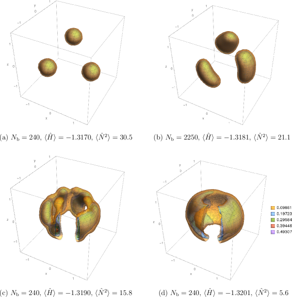
Figure 3: Proton probability density for the lowest-energy, Pauli-allowed state of H${}_{3}^{+}=\{\text{p}^{+},\text{p}^{+},\text{p}^{+},\text{e}^{-},\text{e}^{-}\}$, which is the first rotationally excited state ($N=1$) of the zero-point vibration. (a)–(b) non-projected (symmetry breaking) FECGs; (c)–(d) FECGs approximately projected onto the $(N=1,p=-1)$ irrep of $O(3)$ using 4 and 8 quadrature points for each Euler angle, respectively Muolo et al. (2018a). For the exact wave function $\langle\hat{N}^{2}\rangle=2$ ($N=1$). All quantities are given in atomic units.

Figure 1c shows the (convergence of the) proton density obtained with ECG-GVR functions for the lowest-energy rotational ($N=1$) state which corresponds to the lowest-energy Pauli-allowed state of the system. Notice the significant amount of density at the origin (center of mass) and the large deviations of results obtained with different basis set sizes, which must be artifacts due to incomplete convergence (compare with Figures 3 and 5). The ‘best’ (lowest) five-particle energy, we obtained with an ECG-GVR representation for the lowest-energy state ($N=1$), is 1.8 mE${}_{\text{h}}$ larger than the best estimate on a potential energy surface (PES) Muolo et al. (2018a).

Hence, the slow convergence of the energy and the density in the ECG-GVR ansatz is related to the fact that these functions are not flexible enough to efficiently describe the triangular arrangement (and vibrations) of the protons in H${}_{3}^{+}$ and the spherical symmetry of the system at the same time Muolo et al. (2018a). In principle, it would be possible to define ECG-GVRs with multiple global vectors which could give a better account of the rotational and the multi-particle clustering effects in a polyatomic molecule, but the formalism would be very involved.

II.2 ECGs with three pre-exponential polynomials

We note in passing that, in 2005, Bednarz, Bubin, and Adamowicz proposed an ECG ansatz for H${}_{3}^{+}$ Bednarz et al. (2005),

$$\psi^{[0,0]}_{\text{ECG-3r}}(\boldsymbol{r};\boldsymbol{A},k_{12},k_{13},k_{23}) =r_{12}^{2k_{12}}r_{13}^{2k_{13}}r_{23}^{2k_{23}}\exp\left[-\boldsymbol{r}^{\text{T}}(\boldsymbol{A}\otimes I_{3})\boldsymbol{r}\right]\;,$$ (8)

by including polynomial pre-factors for all three proton-proton distances, $r_{ij}=|\boldsymbol{r}_{i}-\boldsymbol{r}_{j}|$ $(i,j=1,2,3,j>i)$. The integral expressions have been formulated, but to our best knowledge, they have never been used in practical calculations due to their very complicated form and numerical instabilities Bubin et al. (2016).

II.3 Floating ECGs with explicit projection

Floating ECGs (FECGs),

$$\psi_{\text{FECG}}(\boldsymbol{A},\boldsymbol{s};\boldsymbol{r})=\exp\left[-(\boldsymbol{r}-\boldsymbol{s})^{\text{T}}(\boldsymbol{A}\otimes I_{3})(\boldsymbol{r}-\boldsymbol{s})\right]\;,$$ (9)

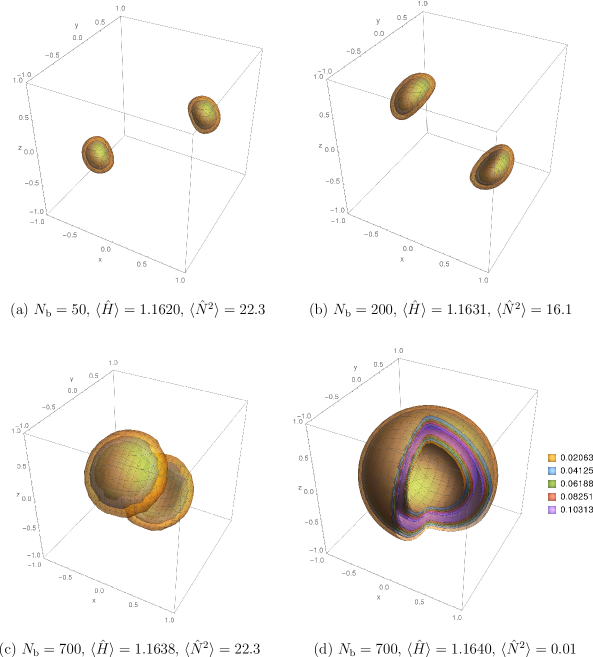
Figure 2: Proton probability density for the ground state of H${}_{2}=\{\text{p}^{+},\text{p}^{+},\text{e}^{-},\text{e}^{-}\}$ $(S_{\text{e}}=0,S_{\text{p}}=0)$ obtained with floating ECGs. (a)–(c): non-projected (symmetry breaking) FECGs; (d) FECG basis functions numerically projected onto the $(N=0,p=+1)$ irrep of $O(3)$ using 22 quadrature points for each Euler angle Muolo et al. (2018a). $N_{\text{b}}$ is the number of basis functions. The energy and the square of the total angular momentum operator are $\langle\hat{H}\rangle=-1.164\,025\,031$ $\text{E}_{\text{h}}$ Pachucki and Komasa (2009) and $\langle\hat{N}^{2}\rangle=0$, respectively. All quantities in the figure are given in atomic units.

offer the flexibility to choose (optimize) not only the exponents but also the centers, $\boldsymbol{s}\in\mathbb{R}^{N_{\text{p}}\times 3}$, which allows one to efficiently describe localization of the heavy particles in polyatomics. At the same time, the FECG functions with arbitary, $\boldsymbol{s}\neq\boldsymbol{0}$, centers do not transform as the irreducible representations (irreps) of the three-dimensional rotation-inversion group, $O(3)$, and therefore, they are neither eigenfunctions of the total squared angular momentum operator, $\hat{N}^{2}$, nor of space inversion (parity). Although these symmetry properties are numerically recovered during the course of the variational optimization converging to the exact solution (see Figures 2a–c and 3a–b), it is extremely inefficient (impractical) for molecular calculations to recover the continuous symmetry numerically.

In order to speed up the slow convergence in the FECG ansatz due to the broken spatial symmetry, we proposed last year Muolo et al. (2018a) to project the floating ECG basis functions onto irreps of $O(3)$,

$$\psi_{\text{p-FECG}}^{[N,p]}(\boldsymbol{A},\boldsymbol{s};\boldsymbol{r})=\frac{1}{4\pi}\int \left[D^{(N)}_{M_{N}M_{N}}(\Omega)\right]^{\ast}\hat{R}(\Omega)\ \frac{1}{2}(1+p\cdot\hat{i})$$

$$\quad\quad\exp\left[-(\boldsymbol{r}-\boldsymbol{s})^{\text{T}}(\boldsymbol{A}\otimes I_{3})(\boldsymbol{r}-\boldsymbol{s})\right]\text{d}\Omega\ \;,$$ (10)

where $\Omega$ collects parameterization of the 3-dimensional rotation, e.g., in terms of three Euler angles, $D^{(N)}_{M_{N}M_{N}}(\Omega)$ is the $(M_{N},M_{N})$th element of the $N$th-order Wigner $D$ matrix, and $\hat{R}(\Omega)$ is the corresponding three-dimensional rotation operator. $p$ is the parity, $+1$ or $-1$, and $\hat{i}$ is the 3-dimensional space-inversion operator. Both the $\hat{R}$ rotational and the $\hat{i}$ space-inversion operators act on the particle coordinates, $\boldsymbol{r}$, but the mathematical form of the ECGs allowed us to translate their action onto the transformation of the ECG parameters, $\boldsymbol{A}$ and $\boldsymbol{s}$ Mátyus and Reiher (2012); Muolo et al. (2018a).

For the projected basis functions the integral expressions of the non-relativistic operators are in general not known analytically, and for this reason, we have carried out an approximate, numerical projection in Ref. Muolo et al. (2018a). Using numerically projected floating ECGs we achieved to significantly improve upon the five-particle energy for H${}_{3}^{+}$ and to approach the current best estimate (on a potential energy surface) for the Pauli-allowed ground state within 70 cm^-1 (with extrapolation within 31 cm^-1).

Properties of (unprojected, symmetry-breaking) and (approximately) projected FECGs are shown for the example of the proton density of H₂ and H${}_{3}^{+}$ in Figures 2 and 3, respectively. At the beginning of an unprojected calculation, the proton density first localizes at around three (two) lobes which corresponds to the localization of the protons in H${}_{3}^{+}$ (and H₂) exhibiting small-amplitude vibrations in a fixed orientation (which can be understood as a superposition of several eigenstates with different $N,M_{N}$, and $p$ values). Then, during the course of the variational increase of the basis set, the spherical symmetry is recovered but the triangular (dumbbell-like) relative configuration of the protons in H${}_{3}^{+}$ (in H₂) is also described within the proton shells (not shown in the figures). Numerical projection reconstructs the expected spherical symmetry directly, without the need of variational optimization, as it is shown in Figures 3c–d and in Figure 2d.

To construct the density plots, we had to evaluate the proton density at several points in space, which is demanding for H${}_{3}^{+}$ with the current projection scheme. For this reason, the largest basis set used for the density plot (Figure 3d) is smaller than the best one obtained during the convergence of the five-particle energy in Ref. Muolo et al. (2018a). Projected FECGs are promising candidates for solving H${}_{3}^{+}$ as a five-particle problem and we anticipate further progress along this line in the future.

II.4 Complex ECGs

In 2006, Bubin and Adamowicz Bubin and Adamowicz (2006) proposed to use ECGs with complex parameters (CECGs),

$$\psi_{\text{CECG}}(\boldsymbol{C};\boldsymbol{r})=\exp\left[-\boldsymbol{r}^{\text{T}}(\boldsymbol{C}\otimes I_{3})\boldsymbol{r}\right]\;,$$ (11)

to describe vibrational ($N=0$, $p=+1$) states of molecules. $\boldsymbol{C}=\boldsymbol{A}+\text{i}\boldsymbol{B}\in\mathbb{C}^{N_{\text{p}}\times N_{\text{p}}}$ is a complex-valued matrix with the real, symmetric matrices, $\boldsymbol{A}$ and $\boldsymbol{B}$. To ensure square integrability, $\psi$ must decay to zero at large distances. Furthermore, to have a positive definite $\psi$, $\boldsymbol{A}$ must be positive definite. Most physical operators have very simple integrals in this basis set and the integrals can be evaluated with a small number of operations (i.e., at low computational cost), which does not increase with increasing the number of nodes of the basis function (unlike for ECG-GVR or polynomial ECG). The rich nodal structure of CECGs, introduced by the $\boldsymbol{B}$ imaginary part of the exponent, can be understood through the Euler identity, $\text{e}^{-(a+\text{i}b)r^{2}}=\text{e}^{-ar^{2}}[\cos(br^{2})-\text{i}\sin(br^{2})]$.

In 2008, Bubin and Adamowicz Bubin and Adamowicz (2008) proposed to extend CECGs for computing $N=1$ states of diatomics with

$$\psi_{\text{zCECG}}(\boldsymbol{C};\boldsymbol{r})=\rho_{z}\exp\left[-\boldsymbol{r}^{\text{T}}(\boldsymbol{C}\otimes I_{3})\boldsymbol{r}\right]\;,$$ (12)

using $\rho_{z}=(\boldsymbol{r}_{n_{1}}-\boldsymbol{r}_{n_{2}})_{z}$, which is the $z$-component of the displacement vector between the two nuclei, $n_{1}$ and $n_{2}$. This ansatz yields a very good description for the first rotationally excited state of a diatomic molecule (the electrons’ contribution to the total angular momentum is almost negligible).

The analytic matrix elements for the overlap, kinetic energy, Coulomb potential energy, and particle density (together with the energy gradients with respect to the $\boldsymbol{C}$ matrix parameters) have been derived by Bubin and Adamowicz and the expressions can be found in Refs. Bubin and Adamowicz (2006, 2008).

Widespread application of the CECG basis-function family is hindered by the fact that matrix operations (matrix inversion, etc.) are more affected by numerical instabilities in finite (double) precision complex arithmetics when compared to real arithmetics.

Earlier this year, Varga proposed Varga (2019) a numerically stable implementation of the CECG functions, through real combinations,

$$\psi_{\text{C-CECG}}(\bm{r};\boldsymbol{C}) =\frac{1}{2}\big{[}\psi_{{\text{CECG}}}(\bm{r};\boldsymbol{C})+\psi_{{\text{CECG}}}(\bm{r};\boldsymbol{C}^{\ast})\big{]}\;,$$ (13)

$$\psi_{\text{S-CECG}}(\bm{r};\boldsymbol{C}) =\frac{1}{2\text{i}}\big{[}\psi^{{\text{CECG}}}(\bm{r};\boldsymbol{C})-\psi^{{\text{CECG}}}(\bm{r};\boldsymbol{C}^{\ast})\big{]}$$ (14)

with $\boldsymbol{C}^{\ast}$ being the complex conjugate of $\boldsymbol{C}$, which allowed him to work with real-valued Hamiltonian and overlap matrices. Furthermore, he also proposed an imaginary-time propagation approach to make the optimization of the complex exponent matrices efficient for the ground state of molecular systems Varga (2019).

III Algorithm for numerically stable calculations with complex ECGs

In this section, we present the key elements of a numerically stable algorithm that we developed for the original (complex) CECG functions.

Following Eq. (12), we define a new CECG basis function by specifying the $\boldsymbol{A}$ and $\boldsymbol{B}\in\mathbb{R}^{N_{\text{p}}\times N_{\text{p}}}$ real symmetric matrices, which give the complex symmetric matrix, $\bm{C}={\bm{A}}+\text{i}\,{\bm{B}}$, in the exponent of the ECG. We work in laboratory-fixed Cartesian coordinates (LFCC) Simmen et al. (2013); Muolo et al. (2018b) and use a multi-channel optimization procedure, i.e., optimize the coefficient matrices corresponding to different translationally invariant (TI) Cartesian coordinate coordinate representations Muolo et al. (2018b). Owing to the mathematical form of the ECGs, the transformation of the coordinates can be translated to the transformation of the parameter matrix Mátyus and Reiher (2012). In all TI representations, the $\boldsymbol{A}$ and $\boldsymbol{B}$ matrices are block diagonal, i.e., the TI and the center-of-mass (CM) blocks do not couple. To ensure square integrability, we choose the CM block of $\boldsymbol{A}$ to have non-zero values on its diagonal. We choose the same non-zero value for all diagonal entries and for each basis function, the contribution of which is eliminated (subtracted) during the evaluation of the integrals. With this choice for the real part $\boldsymbol{A}$, we are free to set the CM block of the imaginary part $\boldsymbol{B}$ to zero, and $\psi$, of course, remains positive definite (due to the non-vanishing CM block of $\boldsymbol{A}$).

In order to obtain $N=1$ states, we use CECGs multiplied with the $z$ coordinate of a ‘pseudo-particle’. Bubin and Adamowicz used the $z$ component of the nucleus-nucleus displacement vector in diatomic molecules Bubin and Adamowicz (2008). We do not choose only a single pseudo-particle but pick different particle pairs for the different basis functions (and possibly several other linear combinations of the particle coordinates, inspired by the ECG-GVR idea Varga et al. (1998b)) to ensure that the contribution of each particle pair to the angular momentum is accounted for. Hence, our general form for complex basis functions, gzCECG, for $N=1,p=-1$ states is

$$\phi_{\text{gzCECG}}(\boldsymbol{r};\boldsymbol{C},i)=\rho^{(i)}_{z}(\bm{r})\,\exp\left[-\bm{r}^{T}(\boldsymbol{C}\otimes\boldsymbol{I}_{3})\bm{r}\right]~{},$$ (15)

where $\rho^{(i)}_{z}$ is the $z$ component of the $i$th translationally invariant vector, formed as a linear combination of the particle coordinates

$$\rho^{(i)}_{z}(\bm{r})=\sum_{j=1}^{N_{\text{p}}}u^{(i)}_{j}r_{j,z}\;.$$ (16)

Of course, there are infinitely many such combinations. In the present calculations, we have included all possible pairs of particles, i.e., $i$ in Eq. (16) cycles through the possible particle pairs only. For example, there are $\left(\begin{array}[]{c}5\\ 2\end{array}\right)=10$ possible particle pairs in H${}_{3}^{+}$, and we consider the following $\rho_{z}^{(i)}$-parameterization ($i=1,2,\ldots,10$) in the gzCECG representation:

1. $\boldsymbol{u}^{(1)}=(1,-1,0,0,0)$

2. $\boldsymbol{u}^{(2)}=(1,0,-1,0,0)$

4. $\boldsymbol{u}^{(10)}=(0,0,0,1,-1)$.

A robust and numerically stable implementation of (gz)CECGs has been a challenging task. The overlap and Hamiltonian matrix elements are complex and the complex generalized eigenvalue problem quickly becomes unstable when increasing the size of the basis set in a stochastic variational approach. We have studied the nature of these instabilities and have identified two ingredients producing this unstable behavior.

First, an unrestricted optimization of the $\boldsymbol{B}$ matrix generates increasingly oscillatory functions, and thus the basis function decays slowly in the limit $\bm{r}\rightarrow\infty$. This behavior affects a broad region of the parameter space; it happens, whenever the imaginary part $\boldsymbol{B}$ dominates the real part $\boldsymbol{A}$.

Second, the analytic overlap and Hamiltonian matrix elements require the calculation of the determinant and the inverse of the complex, symmetric matrix $\boldsymbol{C}$, the evaluation of which suffer from loss of precision in floating-point arithmetics, i.e., an ill-conditioned matrix is still invertible, but the inversion is numerically unstable. The quality of the eigenvalues and eigenfunctions of the Hamiltonian matrix (with the complex, non-diagonal overlap matrix) is thereby compromised by ill-conditioned matrices $C$, an undesired feature which can be identified by repeating the calculations with higher-precision arithmetics or by monitoring the range spanned by the eigenvalues of the matrices .

Based on these observations, we propose the following conditions to ensure numerical stability of the variational procedure in finite-precision arithmetics. During the course of the variational selection and optimization of the basis function parameters, we monitor

1. the ratio of the diagonal elements of the real and the imaginary parts of $\boldsymbol{C}=\boldsymbol{A}+\text{i}\boldsymbol{C}$: $A_{ii}/B_{ii}<\epsilon_{1i},\ i=1,\ldots,N_{\text{p}}\;;$

2. the condition number of $\boldsymbol{C}$: $\kappa(\boldsymbol{C})<\epsilon_{2}\;;$

3. the condition number of the (complex symmetric) $\boldsymbol{S}$ overlap and the $\boldsymbol{H}$ Hamiltonian matrices: $\kappa(\boldsymbol{S})<\epsilon_{3S}$ and $\kappa(\boldsymbol{H})<\epsilon_{3H}\;.$

For acceptance of a trial basis function as a new basis function in the basis set these three conditions must be fulfilled in addition to minimization of the energy. In this way, the numerical stability of the computational procedure can be ensured. For the present calculations, carried out using double precision arithmetics, we have found that the same $\epsilon_{1i}=\epsilon_{2}=\epsilon_{3S}=\epsilon_{3H}=\epsilon=10^{10}$ value for each condition ensures numerical stability for the desired precision, i.e., 6–9 significant digits in the energy. The conditions (1)–(3) and the selected value of $\epsilon$ have been constantly tested during the calculations by solving the linear variational problem within the actual basis set with increased (quadruple and beyond) precision arithmetics.

The first two conditions ensure that the parameter optimization algorithm avoids the regions which would result in overly oscillatory basis functions at large distances, while the third condition controls the level of linear dependency within the (non-orthogonal) basis set.

The computational bottleneck of the (gz)CECG calculations is related to the solution of the generalized complex eigenvalue problem as it was also noted in Ref. Bubin et al. (2016). For this reason, we have implemented and used the FEAST eigensolver algorithm Polizzi (2009), which is a novel, powerful iterative eigensolver for the generalized, complex, symmetric eigenvalue problem.

Figure 4 shows the convergence of the proton density (the energy is also given) for the ground and rotationally and vibrationally excited states of the H₂ molecule ($S_{\text{e}}=0,S_{\text{p}}=0$). These results were obtained within a few days on a multi-core workstation. While the densities are very well converged, the energies can be further improved by subsequent basis-set optimization.

Figure 5 shows our best results obtained for selected states of H${}_{3}^{+}$ ($S_{\text{e}}=0,S_{\text{p}}=1/2$) using the numerically stable gzCECG implementation developed in this work. The proton probability density for the lowest-energy, Pauli-allowed state (zero-point vibration, $N=1$) is well converged, the difference between Figure 5a and Figure 5b can be hardly seen. The best energy is 0.7 mE${}_{\text{h}}\approx 153$ cm^-1 higher than the reference value obtained on a PES pes .

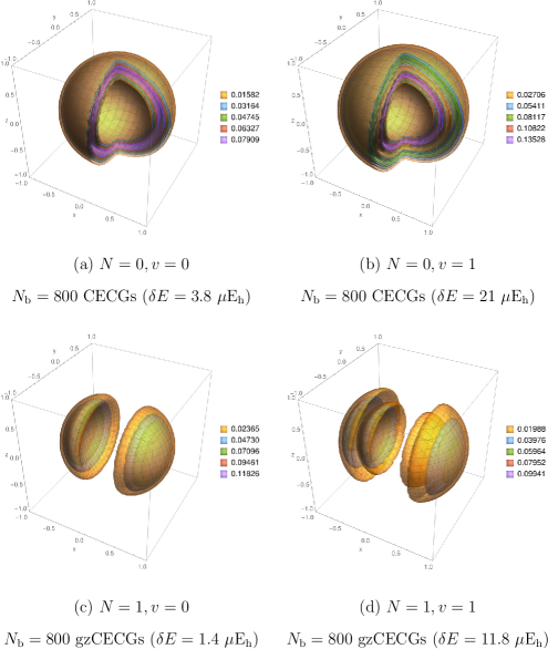
Figure 4: Proton probability density calculated for the ground ($v=0,N=0$) and the lowest rotationally ($N=1$) and vibrationally ($v=1$) excited states of H${}_{2}=\{\text{p}^{+},\text{p}^{+},\text{e}^{-},\text{e}^{-}\}$ ($S_{\text{e}}=0,S_{\text{p}}=(1-N)/2,p=(-1)^{N}$) using (gz)CECG functions. The particle densities are converged within figure resolution, deviation of the energy from benchmark values Pachucki and Komasa (2009) is given in parentheses. All quantities in the figure are given in atomic units.

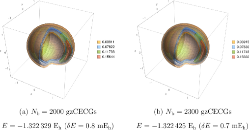
Figure 5: Proton probability density for the lowest-energy, Pauli-allowed state of H${}_{3}^{+}$ $(N=1,p=-1,S_{\text{e}}=0,S_{\text{p}}=1/2)$ obtained with gzCECG functions. The density is converged within figure resolution (compare plots a and b), while the deviation of the five-particle energy from the best value obtained on a PES in our earlier work Muolo et al. (2018a), $E_{\text{ref}}=-1.323\,146\ \text{E}_{\text{h}}$ pes , is given in parentheses ($\delta E=E-E_{\text{ref}}$). All quantities in the figure are given in atomic units.

IV Conclusions

Explicitly correlated Gaussian basis sets have been an excellent choice when aiming for ultra-precise energies for atoms, electron-positron complexes, and diatomic molecules. However, tight convergence of the energy of H${}_{3}^{+}$, the simplest polyatomic system, by including all electrons and protons in a variational procedure has not been achieved yet.

In this work, we critically assessed explicitly correlated Gaussian (ECG) basis sets for solving the molecular (electrons plus nuclei) Schrödinger equation through the study of the convergence of the energy and the particle (proton) density. These observations will contribute to developments that will eventually allow for the convergence of the five-particle energy of H${}_{3}^{+}$ within spectroscopic accuracy, i.e., an uncertainty better than 1 cm^-1 ($<5\times 10^{-6}$ $\text{E}_{\text{h}}$) for the molecular energy.

In 2018, we developed an algorithm for numerically projected floating ECGs Muolo et al. (2018a) to compute the lowest-energy state of H${}_{3}^{+}$ in a variational procedure. In the present work, we presented a numerically stable algorithm for another promising basis set for solving H${}_{3}^{+}$, complex ECGs, which makes it possible to use large basis set sizes in finite precision arithmetics. Although projected floating ECGs provided a somewhat lower energy Muolo et al. (2018a) than complex ECGs (present work) so far, it is currently unclear which type of basis set will finally allow one to reach spectroscopic accuracy for H${}_{3}^{+}$ treated as a five-particle system.

Reaching and transgressing this level of uncertainty in a variational computation will make it possible to directly assess effective non-adiabatic mass models and to study relativistic and quantum electrodynamics effects in the high resolutions spectrum. Such calculations are beyond the scope of the present work and therefore deferred to future studies.

Acknowledgement

This work was supported by ETH Zurich. EM acknowledges financial support from a PROMYS Grant (no. IZ11Z0_166525) of the Swiss National Science Foundation and ETH Zürich for supporting a stay as visiting professor during 2019.

References

- Cheng et al. (2018) C.-F. Cheng, J. Hussels, M. Niu, H. L. Bethlem, K. S. E. Eikema, E. J. Salumbides, W. Ubachs, M. Beyer, N. Hölsch, J. A. Agner, et al., Phys. Rev. Lett. 121, 013001 (2018).
- Markus and McCall (2019) C. R. Markus and B. J. McCall, J. Chem. Phys. 150, 214303 (2019).
- Korobov et al. (2017) V. I. Korobov, L. Hilico, and J. P. Karr, Phys. Rev. Lett. 118, 233001 (2017).
- Alighanbari et al. (2018) S. Alighanbari, M. G. Hansen, V. I. Korobov, and S. Schiller, Nature Physics 14, 555 (2018).
- Wang and Yan (2018) L. M. Wang and Z.-C. Yan, Phys. Rev. A 97, 060501(R) (2018).
- Puchalski et al. (2019) M. Puchalski, J. Komasa, P. Czachorowski, and K. Pachucki, Phys. Rev. Lett. 122, 103003 (2019).
- Hölsch et al. (2019) N. Hölsch, M. Beyer, E. J. Salumbides, K. S. Eikema, W. Ubachs, C. Jungen, and F. Merkt, Phys. Rev. Lett. 122, 103002 (2019).
- Tung et al. (2012) W.-C. Tung, M. Pavanello, and L. Adamowicz, J. Chem. Phys. 136, 104309 (2012).
- Semeria et al. (2016) L. Semeria, P. Jansen, and F. Merkt, J. Chem. Phys. 145, 204301 (2016).
- Mátyus (2018) E. Mátyus, J. Chem. Phys. 149, 194112 (2018).
- Jansen et al. (2018) P. Jansen, L. Semeria, and F. Merkt, J. Chem. Phys. 149, 154302 (2018).
- Stanke et al. (2009) M. Stanke, S. Bubin, and L. Adamowicz, Phys. Rev. A 79, 060501R (2009).
- Herman and Asgharian (1966) R. M. Herman and A. Asgharian, J. Mol. Spectrosc. 19, 305 (1966).
- Herman and Ogilvie (1998) R. M. Herman and J. F. Ogilvie, Adv. Chem. Phys. 103, 187 (1998).
- Bunker and Moss (1977) P. R. Bunker and R. E. Moss, Mol. Phys. 33, 417 (1977).
- Bunker and Moss (1980) P. R. Bunker and R. E. Moss, J. Mol. Spectrosc. 80, 217 (1980).
- Pachucki and Komasa (2009) K. Pachucki and J. Komasa, J. Chem. Phys. 130, 164113 (2009).
- Scherrer et al. (2017) A. Scherrer, F. Agostini, D. Sebastiani, E. K. U. Gross, and R. Vuilleumier, Phys. Rev. X 7, 031035 (2017).
- Schwenke (2001) D. W. Schwenke, J. Phys. Chem. A 105, 2352 (2001).
- Przybytek et al. (2017) M. Przybytek, W. Cencek, B. Jeziorski, and K. Szalewicz, Phys. Rev. Lett. 119, 123401 (2017).
- Mátyus and Teufel (2019) E. Mátyus and S. Teufel, J. Chem. Phys. 150, 214303 (2019).
- Muolo et al. (2018a) A. Muolo, E. Mátyus, and M. Reiher, J. Chem. Phys. 149, 184105 (2018a).
- Bubin and Adamowicz (2006) S. Bubin and L. Adamowicz, J. Chem. Phys. 124, 224317 (2006).
- Bubin and Adamowicz (2008) S. Bubin and L. Adamowicz, J. Chem. Phys. 128, 114107 (2008).
- Suzuki and Varga (1998) Y. Suzuki and K. Varga, Stochastic Variational Approach to Quantum-Mechanical Few-Body Problems (Springer-Verlag, Berlin, 1998).
- Mitroy et al. (2013) J. Mitroy, S. Bubin, W. Horiuchi, Y. Suzuki, L. Adamowicz, W. Cencek, K. Szalewicz, J. Komasa, D. Blume, and K. Varga, Rev. Mod. Phys. 85, 693 (2013).
- Bubin et al. (2013) S. Bubin, M. Pavanello, W.-C. Tung, K. L. Sharkey, and L. Adamowicz, Chem. Rev. 113, 36 (2013).
- (28) Spectroscopic accuracy is generally defined as obtaining (ro)vibrational state energies within better than a 1 cm-1 uncertainty.
- Mátyus and Reiher (2012) E. Mátyus and M. Reiher, J. Chem. Phys. 137, 024104 (2012).
- Lindsay and McCall (2001) C. M. Lindsay and B. J. McCall, J. Mol. Spectrosc. 210, 60 (2001).
- Bunker and Jensen (1998) P. R. Bunker and P. Jensen, Molecular symmetry and spectroscopy, 2nd Edition (NRC Research Press, Ottawa, 1998).
- Mátyus et al. (2011a) E. Mátyus, J. Hutter, U. Müller-Herold, and M. Reiher, Phys. Rev. A 83, 052512 (2011a).
- Mátyus et al. (2011b) E. Mátyus, J. Hutter, U. Müller-Herold, and M. Reiher, J. Chem. Phys. 135, 204302 (2011b).
- Schild (2019) A. Schild, Front. Chem. doi:10.3389/fchem.2019.00424 (2019).
- Suzuki et al. (1998) Y. Suzuki, J. Usukura, and K. Varga, J. Phys. B: At. Mol. Opt. Phys. 31, 31 (1998).
- Armour et al. (2005) E. A. G. Armour, J.-M. Richard, and K. Varga, Phys. Rep. 413, 1 (2005).
- Varga et al. (1998a) K. Varga, J. Usukura, and Y. Suzuki, Phys. Rev. Lett. 80, 1876 (1998a).
- Mátyus (2013) E. Mátyus, J. Phys. Chem. A 117, 7195 (2013).
- (39) D. Ferenc and E. Mátyus, Precise computation of rovibronic resonances of molecular hydrogen: inner-well rotational states. arXiv:1904.08609.
- (40) These reference values have been computed in our earlier work Muolo et al. (2018a) using the GENIUSH program Mátyus et al. (2009); Fábri et al. (2011); Mátyus et al. (2014) with the Polyansky–Tennyson Polyansky and Tennyson (1999) mass model and the GLH3P PES Pavanello et al. (2012) by switching off the relativistic corrections.
- Kinghorn and Adamowicz (1999) D. B. Kinghorn and L. Adamowicz, J. Chem. Phys. 110, 7166 (1999).
- Bubin and Adamowicz (2003) S. Bubin and L. Adamowicz, J. Chem. Phys. 118, 3079 (2003).
- Cafiero et al. (2003) M. Cafiero, S. Bubin, and L. Adamowicz, Phys. Chem. Chem. Phys. 5, 1491 (2003).
- Bednarz et al. (2005) E. Bednarz, S. Bubin, and L. Adamowicz, Mol. Phys. 103, 1169 (2005).
- Bubin et al. (2016) S. Bubin, M. Formanek, and L. Adamowicz, Chem. Phys. Lett. 647, 122 (2016).
- Varga (2019) K. Varga, Phys. Rev. A 99, 012504 (2019).
- Simmen et al. (2013) B. Simmen, E. Mátyus, and M. Reiher, Mol. Phys. 111, 2086 (2013).
- Muolo et al. (2018b) A. Muolo, E. Mátyus, and M. Reiher, J. Chem. Phys. 148, 084112 (2018b).
- Varga et al. (1998b) K. Varga, Y. Suzuki, and J. Usukura, Few-Body Systems 24, 81 (1998b).
- Polizzi (2009) E. Polizzi, Phys. Rev. B 79, 115112 (2009).
- Mátyus et al. (2009) E. Mátyus, G. Czakó, and A. G. Császár, J. Chem. Phys. 130, 134112 (2009).
- Fábri et al. (2011) C. Fábri, E. Mátyus, and A. G. Császár, J. Chem. Phys. 134, 074105 (2011).
- Mátyus et al. (2014) E. Mátyus, T. Szidarovszky, and A. G. Császár, J. Chem. Phys. 141, 154111 (2014).
- Polyansky and Tennyson (1999) O. L. Polyansky and J. Tennyson, J. Chem. Phys. 110, 5056 (1999).
- Pavanello et al. (2012) M. Pavanello, L. Adamowicz, A. Alijah, N. F. Zobov, I. Mizus, O. L. Polyansky, J. Tennyson, T. Szidarovszky, and A. G. Császár, J. Chem. Phys. 136, 184303 (2012).