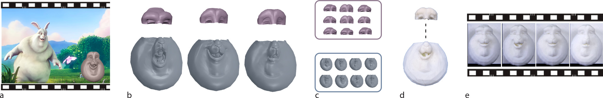
Figure 1. Given an input mesh-animation sequence (a), our system segments and deforms the 3D mesh into parts that can be seamlessly joined (b). Each part is independently used to compute a replacement library, representative of the deforming part in the input (c). StopShop iteratively optimizes the library and a mapping from each frame of the input animation to the pieces in the library. Libraries are 3D printed and each frame is assembled according to the optimized mapping (d). Filmed in sequence, the animation is realized as a stop motion film (e).

A system for efficient 3D printed stop-motion face animation

Abstract.

Computer animation in conjunction with 3D printing has the potential to positively impact traditional stop-motion animation. As 3D printing every frame of a computer animation is prohibitively slow and expensive, 3D printed stop-motion can only be viable if animations can be faithfully reproduced using a compact library of 3D printed and efficiently assemblable parts. We thus present the first system for processing computer animation sequences (typically faces) to produce an optimal set of replacement parts for use in 3D printed stop-motion animation. Given an input animation sequence of topology invariant deforming meshes, our problem is to output a library of replacement parts and per-animation-frame assignment of the parts, such that we maximally approximate the input animation, while minimizing the amount of 3D printing and assembly. Inspired by current stop-motion workflows, a user manually indicates which parts of the model are preferred for segmentation; then, we find curves with minimal deformation along which to segment the mesh. We then present a novel algorithm to zero out deformations along the segment boundaries, so that replacement sets for each part can be interchangeably and seamlessly assembled together. The part boundaries are designed to ease 3D printing and instrumentation for assembly. Each part is then independently optimized using a graph-cut technique to find a set of replacements, whose size can be user defined, or automatically computed to adhere to a printing budget or allowed deviation from the original animation. Our evaluation is threefold: we show results on a variety of facial animations, both digital and 3D printed, critiqued by a professional animator; we show the impact of various algorithmic parameters; and compare our results to naive solutions. Our approach can reduce the printing time and cost significantly for stop-motion animated films.

1. Introduction

Stop-motion is a traditional animation technique that moves a physcial object in small increments between photographed frames, to produce the illusion of fluid motion. As with animation in general, arguably the most expressive part of a character is its face. Extensive use of clay replacement libraries for dialogue and facial expressions, goes back as far as The New Gulliver 1935. The use of a replacement library has become the standard approach to the stop-motion animation of expressive deformable objects, in particular for facial animation. With the advent of 3D printing, replacement animation has become a bridge between the disparate worlds of digital computer animation and physical stop-motion, and is increasingly used as the preferred technique for producing high-quality facial animation in stop motion film [Priebe, 2011].

Faces and 3D models in general are created digitally (or physically sculpted and scanned) to produce a replacement library that covers the expressive range of the 3D model. This library, typically containing thousands of variations of a deformable model is then 3D printed and cataloged. Additional post-processing may be required, including sanding down edges, smoothing inconsistencies, and hand painting the 3D prints. The replacement library is then ready to be used in stop-motion sequences [Alger et al., 2012]. Alternately, the 3D model could be entirely computer animated, and each animation frame of the model independently 3D printed and post-processed for use on a physical set.

In either case, the cost in terms of printing and post-processing time, material, storage and money is prohibitive. Each character of Laika’s stop-motion feature film Coraline could have as many as 15,000 faces and up to 250,000 facial expressions [Kolevsohn, 2009]. Paranorman required 8308 pounds of printer powder, and 226 gallons of ink over the course of production [Priebe, 2011] (see Figure 2). This current practice for character faces (let alone complete 3D models) is expensive for large film studios and completely beyond the reach of independent filmmakers.

Due to the tedious nature of physically moving or replacing objects in the scene for each frame, stop motion objects are typically animated at a lower framerate (often "on twos” or every other frame). Some films, such as Aardman’s Flushed Away or Blue Sky’s The Peanuts Movie, even opt to simulate the aesthetic appeal of stop-motion entirely, via computer animation. As evident by these films, the slight choppiness and lower framerate can be an intentional artistic decision. Our research addresses both 3D printing costs and animation aesthetic, providing users with a system that can produce animation sequences in a stop-motion style digitally, or physically with minimal 3D printing, saving printing time and material.

We present an end-to-end solution designed to optimize the 3D printing of a replacement library of a deformable 3D object, such that high-quality stop-motion approximations of input computer animations can be assembled from that library (see Figure 1). At the core of our system is an optimization problem (Section 3.3) whose solution provides an optimal replacement library to be 3D printed and a per-animation-frame assignment of pieces from this library to reconstruct the input animation faithfully.

As is common with replacement libraries [Priebe, 2011], we can amplify the expressive range of the deformable face/object by first segmenting it into multiple parts. A user specifies the approximate location of the parts, and we calculate boundaries that have minimal or zero deformation between them. An optimal replacement library is then computed independently for each part, and the object assembled by interchangeably combining pieces from each part’s library. The replacement library pieces also need to be instrumented with connectors before 3D printing, so that repeated object re-assembly for stop-motion, is quick and sturdy.

We propose a series of algorithms to assist in the process of creating a library of mix-and-matchable printable pieces and a set of assembly instructions to recreate a given mesh-animation sequence. In particular, we introduce: a novel mesh segmentation method to find near-stationary part boundaries, a deformation process to homogenize part boundaries allowing temporal reshuffling of segmented parts, and finally we simultaneously optimize for a replacement library of printable pieces and their assignment to each frame of an input animation.

We evaluate our algorithm in Section 5 by showing compelling results, both digital and 3D printed, and a comparison to a naive approach to the above problem. As shown in our accompanying video, we are able to faithully approximate input animation of cartoon characters as well as high-fidelity computer animation models. In our examples we achieve a $\approx 25x$ saving over printing each frame for animations of $\approx 750$ frames.

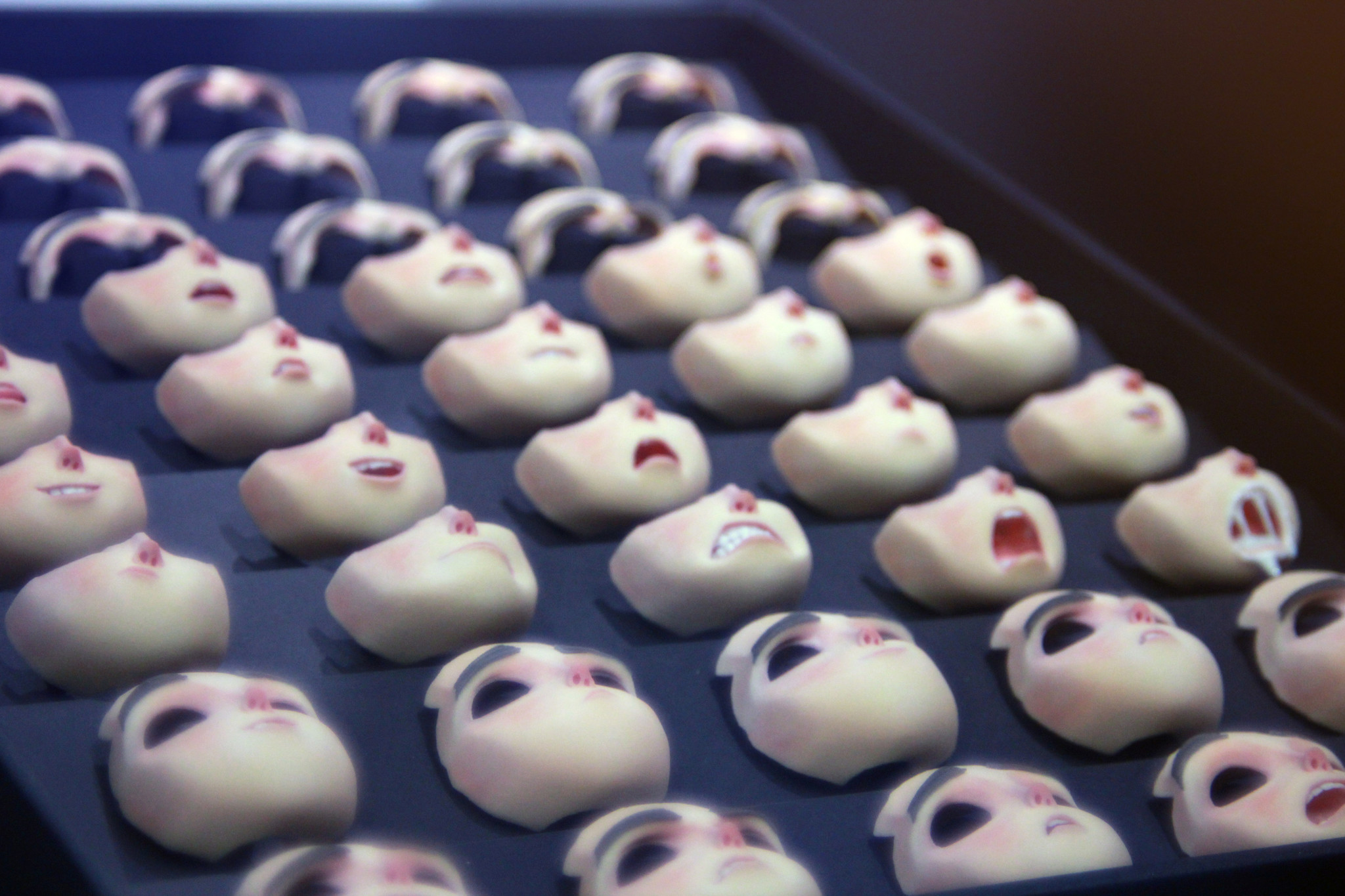
Figure 2. Modern stop-motion films such as Laika’s ParaNorman amass replacement libraries of thousands of 3D printed pieces.

2. Related Work

Our research is inspired by the challenges and animation processes at stop-motion studios like Aardman and Laika [Priebe, 2011], where 3D printing, computer modeling and animation tools are an increasingly indispensible part of the animation workflow. Despite the popularity of stop-motion animation, the topic has received little attention in the computer animation research literature. We thus focus our attention on research topics closest to our problem at an abstract level and those similar in methodology.

Stop-motion

Commercial stop-motion software such as Stop Motion Pro or DragonFrame, focuses on optimized camera controls and convenient interfaces for assembly and review of captured images. There is long history of research on interfaces and techniques for performance animation, such as for paper cut-out animations [Barnes et al., 2008]. Stop-motion armatures have also inspired research into tangible devices [Knep et al., 1995; Bäecher et al., 2016] and interfaces [Singh and Fiume, 1998] for posing and deforming 3D characters. Stop-motion has also been applied to study low fidelity prototyping for user interfaces [Bonanni and Ishii, 2009]. Digital removal of seams and hands from stop-motion images has been addressed by [Brostow and Essa, 2001]. [Han et al., 2014] presented a tool to aid in the generation of motion blur between static frames to show fast motions. However, the problem of generating replacement libraries for the purpose of 3D printed stop motion animation has not been addressed before.

Animation Compression

Although not intentional, stop-motion can be seen as a compression of high-framerate or continuous animation into a much smaller set of frames. In computer graphics and especially computer game development, there have been many methods proposed for compressing animations: for deformable meshes using principal component analysis [Alexa and Müller, 2000; Sattler et al., 2005; Vasa et al., 2014], for articulated characters using skeletal skinning subspaces [James and Twigg, 2005; Le and Deng, 2014], or by analyzing patterns in motion capture data [Gu et al., 2009]. These methods for digital animation are free to define interpolation operations, effectively approximating the input animation with a continuous (albeit high dimensional) function space. Stop motion in contrast requires a discrete selection: a 3D-printed face is either used for this frame or not. We cast this problem of extracting a printed library of shapes and assigning those shapes to each frame of the animation as one of sparse dictionary learning or graph clustering, well studied topics often used in computer graphics. In particular, Le & Deng [2013] use sparse dictionary learning to significantly compress mesh animations, as a weighted combination of a few basis meshes. While their weights are sparse, we must represent every animated frame using a single physical replacement mesh, necessitating a very different optimization strategy.

Stylization

Much of the work in stylizing characters pertains to painterly rendering or caricature [Kyprianidis et al., 2013]. Similar to signature "choppy" style of stop-motion, controllable temporal flickering has been used to approximate the appearance of real hand-painted animation of faces [Fišer et al., 2017] and articulated characters [Dvorožnák et al., 2018]. Video summarization techniques select discrete set of images or clips that best sum up a longer clip, recently using deep learning to select semantically meaningful frames [Otani et al., 2016]. Stop-motion also requires a reduced but typically larger, discrete set of replacement 3D models, not to summarize but to approximate an input animation. Other research in stylizing 3D animation has explored key-pose and motion-line extraction from 3D animations for comic strip like depiction. Stop-motion in contrast, can be imagined as geometry "posterization" along an animation, analogous to the problem of image and video color posterization [Wang et al., 2004], albeit with different objectives. Stop-motion stylization of an animation can be also interpreted as the inverse problem of keyframe in-betweening [Whited et al., 2010], spacetime constraints [Witkin and Kass, 1988], or temporal upsampling [Didyk et al., 2010]. We are inspired by these methods.

Facial Animation

We use replacement library as the principal use case of replacement animation for stop-motion in this paper. Current animation practice typically creates facial animation using blendshapes (convex combinations of posed expressions [Lewis et al., 2014; Ribera et al., 2017]), with layered controls built atop to model emotion and speech [Edwards et al., 2016]. The blendshape weights of a face can provide useful information regarding both the saliency and difference in expression between faces [Ribera et al., 2017], which we exploit when available. Our work is also inspired by work on compression using blendshapes [Seo et al., 2011] and optimization of spatially sparse deformation functions [Neumann et al., 2013]. In contrast, our optimization may be seen as producing an extreme form of temporal sparsity.

Shape segmentation and 3D printing

Our system also automatically segments the geometry of an animated shape in order to maximize expressiveness of the replacement library while maintaining a tight 3D printing material budget. Shape segmentation is a fundamental and well studied problem in geometry processing [Shamir, 2008]. In an animation, most segmentation approaches hunt for rigid or near-rigid parts during animation [Bergou et al., 2007; Lee et al., 2006; Ghosh et al., 2012]. Our problem is orthogonal to these; rather than looking for near-rigid parts, we look for near-motionless boundaries between the segmented parts. Nonetheless, mesh saliency [Jeong and Sim, 2014] or other quality/printability measures [Zhang et al., 2015] could easily be incorporated into our optimization. Segmenting and processing input 3D geometry for high quality 3D printing in general [Luo et al., 2012; Hu et al., 2014; Herholz et al., 2015; Wang et al., 2016] and faces in particular [Noh and Igarashi, 2017] is subject to ongoing research and useful for the final 3D printing of the replacement pieces computed by our system. Instead of printing a replacement library, Bickel et al. [2012] used material optimization methods to create synthetic silicone skin, fabricated using 3D printed molds, for animatronic figures of human faces.

3. System and Algorithm Design

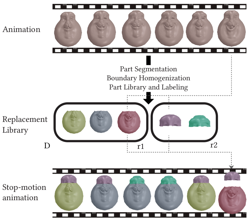
Figure 3. Algorithm overview. Input shape is segmented into parts and each animation frame is smoothly deformed so the cut has the same geometry across all frames. For each part independently, replacement library and corresponding assignment labels to each frame are optimized simultaneously.

The input to our method is an $n$-frame mesh-animation sequence $\mathbf{X}=[\mathbf{x}_{1},\mathbf{x}_{2},…,\mathbf{x}_{n}]∈\mathbb{R}^{m×3×n}$, where $\mathbf{x}_{f}∈\mathbb{R}^{m×3}$ contains the vertex positions of the $f$th animation frame of a mesh with $m$ vertices and $k$ triangles, and $\mathbf{x}_{fi}∈\mathbb{R}^{3}$ is the 3D position of the $i$th vertex in that frame. Multiple temporally disjoint animation clips of the mesh are simply concatenated in $\mathbf{X}$, with the cut locations marked. Please note that we refer to mesh faces as triangles to avoid confusion with the faces being animated, even though our solution applies to quads and other polygons.

We assume the mesh animates via vertex displacements only and does not change topology, connectivity, or number of triangles ($k$) during the animation. The user also inputs a desired number of parts $s$ (e.g., $s=2$ for a face split into top and bottom) and a desired replacement library size $d_{j}\,∀j=1,\dots,s$, indicating the number of printable pieces per part (e.g., $d₁=3,d₂=2$ to output 2 top face pieces and 3 bottom pieces in Figure 3).

The output of our method is $s$ replacement libraries, one for each part containing the correspondingly given number of pieces to 3D print, and a labeling of each of the $n$ input animations frames indicating which piece from each part library to place in order to recreate the frame (see Figure 3).

As enumerated in Figure 3, our method proceeds in three steps: 1) the input shape is segmented into $s$ parts with a minimally noticeable cut, 2) each input frame is smoothly deformed so the segmentation cut across all frames has the same geometry, and, finally, 3) for each part independently, the replacement library and corresponding assignment labels to each frame are optimized simultaneously.

3.1. Part Segmentation

Many deformable objects like faces have localized regions of deformation separable by near rigid boundaries, though the exact location of the cut separating these regions is generally non-planar, curving around features like eyes, cheeks, and noses. Existing stop-motion facial animations often segment a head into an upper and lower face just below the eye-line, optionally with a rigid back of the head. While our approach generalizes (via multi-label graphcut) to $s>2$, our implementation and results focus on the predominant segmentation for faces, with $s=2$.

Our input to this stage is the mesh-animation sequence $\mathbf{X}$, and the output, a new mesh-animation sequence $\mathbf{Y}$ with $y$ triangles and a per-triangle part assignment $\mathbf{p}∈\{1,\dots,s\}^{y}$. The output is geometrically equivalent to the input, but with new vertices and triangles ($y$ triangles instead of the input $k$ triangles) added along a smooth boundary separating the parts.

Users can roughly indicate desired parts by specifying a seed triangle (or set of triangles) $T_{j}$ for each part $j$. We find a per-triangle part assignment $\mathbf{q}_{\alpha}$ for each input triangle $α$ of the average mesh. The boundaries between part regions minimize an energy that penalizes cutting along edges that move significantly during the input animation $\mathbf{X}$:

(1) $$\min_{\mathbf{q}∈\{1,\dots,s\}^{k}} ∑\limits_{α=1}^{k}u(α)+γ∑\limits_{α=1}^{k}∑\limits_{β=1}^{k}b(α,β)$$

where $γ$ balances between the unary and binary terms described below (we use a default of $γ=100$ for 3D models scaled to a unit bounding-box). The unary data term $u(α)$ penalizes parts from straying in distance from the input seeds:

(2) $$u(α) :=\text{dist}(α,T_{j}),\text{ $j=\mathbf{q}_{α}$}$$

where $\text{dist}(α,T_{j})$ measures the geodesic distance from the triangle $α$ to the closest seed in the set $T_{j}$. The binary smoothness term penalizes cuts that pass through shapes that have high displacement from their average position:

(3) $$b(α,β) :=\begin{cases}∑\limits_{f=1}^{n}\|\mathbf{e}_{fαβ}\|\left(1+∑\limits_{i∈α∩β}\|\mathbf{x}_{fi}-\tilde{\mathbf{x}}_{i}\|\right)&\text{ if $q_{α}≠q_{β}$,}\\ 0&\text{ otherwise,}\end{cases}$$

where $\tilde{\mathbf{x}}∈\mathbb{R}^{m×3}$ denotes the average mesh vertex positions across the animation, $\|\mathbf{e}_{fαβ}\|$ is the length of the edge between triangles $α$ and $β$ at frame $f$ and $α∩β$ indicates the indices of the shared vertices on this edge. The $1+$ penalizes long cuts even in non-moving regions.

This energy is efficiently minimized via graphcut-based multilabel approach [Y. Boykov et al., 2001; Kolmogorov and Zabin, 2004; Boykov and Kolmogorov, 2004]. The result is a per-triangle labeling. Since the user manually chooses seed triangles by clicking on the mesh, our optimization needs to be robust to perturbations of the seed triangle placement. Figure 4 shows that we find the same boundary once $\gamma$ is large enough. For a generic mesh, the part boundary may zig-zag due to the necessity of following mesh edges (see Figure 5(b)). This is not only aesthetically disappointing but pragmatically problematic: jagged boundaries will prevent 3D printed parts from fitting well due to printer inaccuracies.

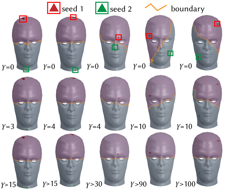
Figure 4. Robustness of the part segmentation method with respect to perturbations of the seed triangle placement. Each column shows a different initialization of seed triangles with the first row showing the extreme case without the binary smoothness term as in Eq. 1. Increasing the influence of the binary term via $\gamma$ produces the same boundary.

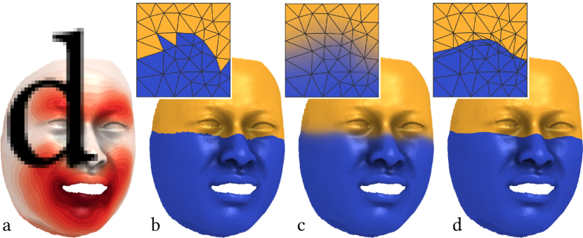
Figure 5. Left to right: average displacement visualized over the average face is converted into a per-triangle segmentation. We smooth this as a scalar per-vertex function and then extract a smoothly bounded segmentation as an iso-contour.

Part boundary smoothing

We smooth per-triangle part boundaries by treating each part as an indicator function ($χ_{j}(\mathbf{x})=1$ if triangle $\mathbf{x}$ is in part $j$, $χ_{j}(\mathbf{x})=0$ otherwise) (see Figure 5). We move each indicator function into a per-vertex quantity (no longer binary) by taking a animation-average-triangle-area-weighted average of $χ_{j}$ triangle values. Treating each per-vertex quantity as interpolated values of a piecewise-linear function defined over the mesh, we mollify each segmentation function by Laplacian smoothing. Because the input indicator functions partition unity, so will the output smoothed functions: each function can be thought of as a point-wise vote for which part to belong to. Finally, the smoothed part boundaries are extracted by meshing the curves that delineate changes in the maximum vote and assigning each (possibly new) triangle to the part with maximum value (after meshing, the maximum is piecewise constant in each triangle). This meshing does not change the geometry of the surface, only adds new vertices f

Note that the number of vertices and triangles on the mesh-animation sequence $\mathbf{Y}$ will likely change from the number of vertices $m$ and triangles $k$ of the input mesh-animation sequence $\mathbf{X}$, as a result of the smooth part boundary extraction. In subsequent steps, for notational simplicity however, we will continue to use $m$ and $k$ to refer to the vertex and face count of the 3D meshes being processed.

3.2. Part Boundary Homogenization

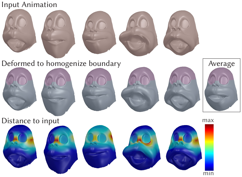
Figure 6. The input mesh-animation sequence is cut into two parts according to the displacement from the average face (inset). Each mesh is then minimally and smoothly deformed so that the part boundary is constant across the animation.

We now deform all frames of the segmented mesh-animation sequence $\mathbf{Y}$, so that the geometry of each frame along the part boundaries is temporally constant (see Figure 6). This will allow us to mix and match different poses for each part while maintaining continuity across the part boundaries (see Figure 7). Given a set of $n$ mesh positions $\mathbf{Y}=[\mathbf{y}_{1},\mathbf{y}_{2},…,\mathbf{y}_{n}]∈\mathbb{R}^{m×3×n}$ and a per-triangle part labeling $\mathbf{p}∈\{1,\dots,s\}^{y}$ as input, we compute a vertex-deformation of these meshes with new positions $\mathbf{Z}=[\mathbf{z}_{1},\mathbf{z}_{2},…,\mathbf{z}_{n}]∈\mathbb{R}^{m×3×n}$.

We find a minimal deformation of the input frames by solving a constrained optimization problem so that the displacements move each vertex $\mathbf{y}_{fi}∈\mathbb{R}^{3}$ along the part boundaries (i.e., vertices incident on triangles with different assignment) to its average value across the input meshes $\tilde{\mathbf{y}}_{i}∈\mathbb{R}^{3}$ and move non-boundary vertices smoothly. We conduct this optimization for each input mesh of the sequence $\mathbf{Y}$. In the continuous setting, we model this as a minimization of the squared-Laplacian energy of the displacement field:

(4) $$\operatorname*{argmin}_{\mathbf{z}_{f}} ∫_{\text{surface}}\|∆(\mathbf{z}_{f}-\mathbf{y}_{f})\|_{F}^{2}\;dA$$

(5) subject to: $$\mathbf{z}_{f}=\tilde{\mathbf{y}}_{f}\text{ along the seam}$$

(6) and $$∇\mathbf{z}_{f}=∇\tilde{\mathbf{y}}\text{ along the seam},$$

where the gradient condition not only ensures a unique solution, but also forces the normal of the resulting meshes to vary consistently. This condition is of practical importance for final fabrication: each part can be extruded inward along its normal direction to create a boundary-matching volumetric (printable) shell.

In practice, we implement this for our discrete triangle meshes using the mixed Finite-Element method [Jacobson et al., 2010] (i.e., squared cotangent Laplacian). We implement the gradient condition by fixing one-ring of vertex neighbors along the seams to their average values as well.

The Laplacian energy (4) is discretized using linear FEM Laplacian $M^{-1}L$ where $M$ is the mass matrix and $L$ is the symmetric cotangent Laplacian of the average mesh.

(7) $$∫_{\text{surface}}||∆(\mathbf{z}_{f}-\mathbf{y}_{f})||_{F}^{2}\;dA =tr((M^{-1}LD)^{T}MM^{-1}LD)$$

(8) $$=tr(D^{T}(L^{T}M^{-1}L)D)$$

(9) $$\text{where }D_{f}:=\begin{cases}\tilde{\mathbf{y}}_{f}-\mathbf{y}_{f}&\text{along seam/one-ring neighbourhood}\\ \mathbf{z}_{f}-\mathbf{y}_{f}&\text{otherwise}\end{cases}$$

The energy term (8) is quadratic in the unkwons $\mathbf{z}_{f}$ and convex with linear equality constraints that is solved using Eigen’s [Guennebaud et al., 2010] sparse Cholesky solver.

Though each frame’s deformation is computed independently, we have modeled this as a smooth process and, thus, the temporal smoothness of the input meshes will be maintained: temporally smooth input animations remain smooth.

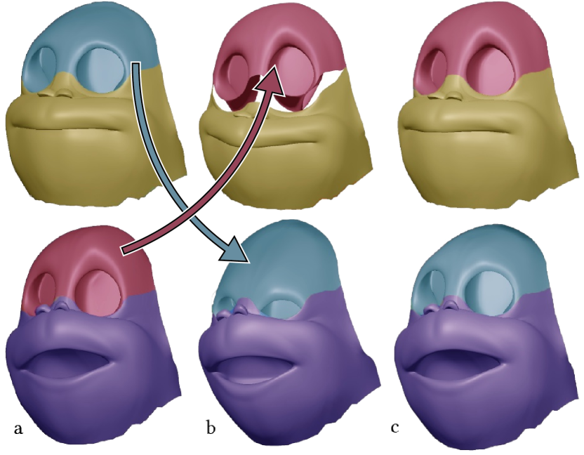
Figure 7. In (a), two input frames (rows) are each segmented into two parts (colors). Simply mixing tops and bottoms of the original meshes leads to boundary mismatches (b). Instead, our system optimizes deformations for each part to homogenize the boundaries, allowing seamless assembly (c).

3.3. Replacement Library and Per-Frame Assignment

Sections 3.1 and 3.2 allow us to maximize the expressivity of a replacement library by segmenting and deforming the input mesh into $s$ parts, whose individual replacement libraries can be arbitrarily assembled together. Replacement libraries for each of the $s$ parts can thus be computed independently. We now focus on determining the pieces that compose the replacement library of each part, and a per-animation-frame assignment of pieces from these libraries to reconstruct the input mesh-animation sequence faithfully.

For brevity of notation, we denote the input to this subroutine as desired library size $d$ and a (sub-)mesh animation of a single part $\mathbf{Z}=[\mathbf{z}₁,\mathbf{z}₂,…,\mathbf{z}_{n}]∈\mathbb{R}^{3m×n}$. We will operate on $\mathbf{Z}$ as a 2D matrix (we stack $x$,$y$, and $z$ coordinates vertically). Optionally, the user may provide a vector $\mathbf{w}∈\mathbb{R}^{m}$ of saliency weights, so that $w_{i}∈\mathbb{R}$ contains a larger (smaller) value if the $i$th vertex is more (less) salient. Saliency can be animator-defined, or computed automatically from criteria, such as frames that are blendshape extremes, motion extrema [Coleman et al., 2008], or viseme shapes [Edwards et al., 2016]. Additionally, as already mentioned, the user may optionally include a “cut” vector $\mathbf{c}∈\{\text{true},\text{false}\}^{n}$ indicating whether each frame is beginning a new unrelated sequence in the animation (e.g., a scene change).

The output is a replacement library of $d$ pieces for the part $\mathbf{R}=[\mathbf{r}_{1},\mathbf{r}_{2},..,\mathbf{r}_{d}]∈\mathbb{R}^{3m×d}$ and a sequence of $n$ labels assigning each input frame to a corresponding piece from the library $\boldsymbol{\ell}=[\ell_{1},\ell_{2},…,\ell_{n}]∈\{1,…,d\}^{n}$. We optimize for $\mathbf{R}$ and $\boldsymbol{\ell}$ to best approximate the input geometry and the change in input (e.g., the discrete velocity) between consecutive frames for inputs that come from animation clips.

Our optimization searches over the continuous space of library pieces and the discrete space of assignment labels, to optimize the combined $L²$ geometry and velocity energy function $E$:

(10) $$\mathop{\text{minimize}}_{\mathbf{R},\boldsymbol{\ell}}\ \underbrace{½||\mathbf{X}-\mathbf{R}\mathbf{S}(\boldsymbol{\ell})||_{\mathbf{W}}^{2}+\frac{λ}{2}||\mathbf{X}\mathbf{G}-\mathbf{R}\mathbf{S}(\boldsymbol{\ell})\mathbf{G}||_{\mathbf{W}}^{2}}_{E(\mathbf{R},\boldsymbol{\ell})},$$

(11) $$\text{where }\mathbf{S}(\boldsymbol{\ell})∈\{0,1\}^{d×n},\mathbf{S}_{kf}(\boldsymbol{\ell}):=\begin{cases}1&\text{if }\ell_{f}=k,\\ 0&\text{otherwise,}\end{cases}$$

where $\mathbf{W}∈\mathbb{R}^{3n×3n}$ is a matrix containing the per-vertex saliency weights $\mathbf{w}$ repeated along the diagonal for each spatial coordinate and $λ$ balances between shape accuracy and velocity accuracy, and $\mathbf{G}∈\mathbb{R}^{n×(n-1)}$ is a sparse matrix computing the temporal forward finite difference:

(12) $$G_{fg}=\begin{cases}\hphantom{-}0&\text{if }\mathbf{c}_{f}\text{ or }\mathbf{c}_{g},\\ \hphantom{-}1&\text{else if }f=g+1,\\ {-}1&\text{else if }f=g,\\ \hphantom{-}0&\text{otherwise.}\end{cases}$$

As opposed to soft labeling [Wright et al., 2010; Elad and Aharon, 2006], our labeling is hard in the sense that the implied stochastic “representation” matrix $\mathbf{S}(\boldsymbol{\ell})$ is binary. We are literally going to print our replacement libraries. This is considerably harder to optimize than the standard sparse dictionary learning problem where sparsity is enforced via an objective term and may be convexified using an $L^{1}$-norm. Instead, we optimize using block coordinate descent. We repeatedly iterate between:

• finding the optimal replacement library pieces $\mathbf{R}$ holding the labels $\boldsymbol{\ell}$ fixed, and

• finding the optimal labels holding the library fixed.

Since fixing the labels $\boldsymbol{\ell}$ also fixes the representation matrix $\mathbf{S}(\boldsymbol{\ell})$, finding the optimal library amounts to minimizing a quadratic least squares energy. The optimal library $\mathbf{R}$ is a solution to a large, sparse linear system of equations:

(13) $$\underbrace{(\mathbf{S}(\boldsymbol{\ell})\mathbf{S}(\boldsymbol{\ell})^{\mathsf{T}}+λ\mathbf{S}(\boldsymbol{\ell})\mathbf{G}\mathbf{G}^{\mathsf{T}}\mathbf{S}(\boldsymbol{\ell})^{\mathsf{T}})}_{\mathbf{A}}\mathbf{R}^{\mathsf{T}}=\underbrace{(\mathbf{S}(\boldsymbol{\ell})+λ\mathbf{S}(\boldsymbol{\ell})\mathbf{G})\mathbf{X}^{\mathsf{T}}}_{\mathbf{B}},$$

Where $\mathbf{A}∈\mathbb{R}^{n×n}$ is a sparse matrix and $\mathbf{B}∈\mathbb{R}^{n×3m}$ is a dense matrix whose columns correspond to specific vertex coordinates. This formula reveals that each vertex-coordinate (column in $\mathbf{R}^{\mathsf{T}}$) is computed independently, hence, the saliency weights $\mathbf{W}$ fall out during differentiation.

As long as $\mathbf{S}(\boldsymbol{\ell})$ contains at least one non-zero entry per-row (i.e., each library instance is used at least once), the system matrix $\mathbf{A}$ can be efficiently factorized (e.g., via Cholesky with reordering) and then applied (e.g., in parallel) to each column of the right-hand side.

Fixing the library $\mathbf{R}$ and optimizing for the labels $\boldsymbol{\ell}$ is more complicated, but nonetheless well posed. We may rewrite the objective function $E$ in Equation (10) as a sum of unary terms involving the independent effect of each label $\boldsymbol{\ell}_{f}$ and binary terms involving the effect of pairs of labels $\boldsymbol{\ell}_{f}$ and $\boldsymbol{\ell}_{g}$ corresponding to the $f$th and $g$th animation frames:

(14) $$E(\mathbf{R},\boldsymbol{\ell}) =∑\limits_{f=1}^{n}\overline{u}(f)+∑\limits_{f=1}^{n}∑\limits_{g=1}^{n}\overline{b}(f,g),$$

where

(15) $$\overline{u}(f) :=½||\mathbf{x}_{f}-\mathbf{r}_{\ell_{f}}||_{\mathbf{W}}^{2},$$

(16) $$\overline{b}(f,g) :=\begin{cases*}\frac{λ}{2}||(\mathbf{x}_{g}-\mathbf{x}_{f})-(\mathbf{r}_{\ell_{g}}-\mathbf{r}_{\ell_{f}})||_{\mathbf{W}}^{2}&\text{if $|f-g|=1$},\\ 0&\text{otherwise.}\end{cases*}$$

The binary term $\overline{b}(f,g)$ satisfies the regularity requirement described by Kolmogorov and Zabin [2004]. Specifically in the case of neighboring animation frames with $|f-g|=1$, the term sastisfies:

(21) $$\footnotesize\begin{array}[]{c}½\|(\mathbf{x}_{g}-\mathbf{x}_{f})-(\mathbf{r}_{\ell_{f}}-\mathbf{r}_{\ell_{f}})\|_{F}^{2}\ +\\ ½\|(\mathbf{x}_{g}-\mathbf{x}_{f})-(\mathbf{r}_{\ell_{g}}-\mathbf{r}_{\ell_{g}})\|_{F}^{2}\end{array} ≤\footnotesize\begin{array}[]{c}½\|(\mathbf{x}_{g}-\mathbf{x}_{f})-(\mathbf{r}_{\ell_{f}}-\mathbf{r}_{\ell_{g}})\|_{F}^{2}\ +\\ ½\|(\mathbf{x}_{g}-\mathbf{x}_{f})-(\mathbf{r}_{\ell_{g}}-\mathbf{r}_{\ell_{f}})\|_{F}^{2}\\ \end{array}$$

which after simplification is equal to

(22) $$0 ≤\|\mathbf{r}_{\ell_{g}}-\mathbf{r}_{\ell_{f}}\|_{F}^{2}.$$

Since Equation (22) is always true we satisfy the regularity requirement for energy to be graph-representable. Problems of this form are efficiently solved using graphcut-based multilabel optimization (e.g., $α$-expansion) [Y. Boykov et al., 2001; Kolmogorov and Zabin, 2004; Boykov and Kolmogorov, 2004].

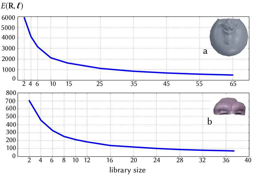
Figure 8. Increasing the number of pieces improves accuracy of the approximation but increases the cost of printing.

When we set the velocity term weight to zero ($λ=0$), graphcut becomes unnecessary: optimizing labels becomes a simple closest point problem, and optimizing for the library becomes a simple center of mass computation. Without the velocity term, our block coordinate descent thus, reduces to Lloyd’s method for solving the $k$-means clustering problem [Lloyd, 1982]. In other words, for $λ>0$ we solve a generalization of the $k$-means clustering problem, and like $k$-means, our objective landscape is non-convex with many local minima. Our optimization deterministically finds a local minimum given an intial guess. We thus run multiple instances of our algorithm, with random initial assignments and keep the best solution Figure 9.

We now discuss practical workflow scenarios and how they fit into the above algorithm.

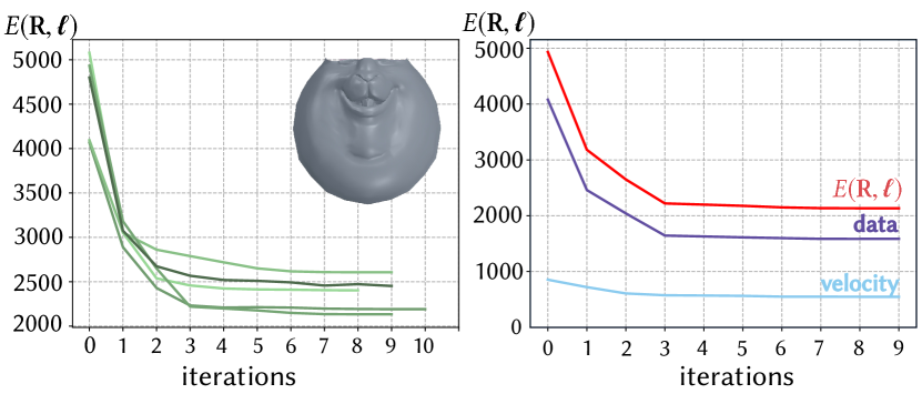
Figure 9. Left: the total labeling energy $E(\mathbf{R},\boldsymbol{\ell})$ (integrated over 766 frames and 5826 vertices) for multiple runs of the block coordinate descent algorithm on a bunny sequence, 25 labels and $λ=2$ to approximate the lower part of the bunny. On average, the difference between a vertex on the input frame and its corresponding vertex on the library piece is 0.11mm, and its per-frame velocity difference is 0.04mm. The bunny model was scaled to be $2\times 2.5\times 1.42$ cm, similar to printing results shown in the accompanying video. Right: single iteration of the block coordinate descent algorithm showing the data and velocity terms separately.

Pre-defined replacement library

Sometimes the entire library or part of it may be fixed, for example if it was previously printed for a film prequel. Our algorithm can trivially be used for labeling a fixed library to input animation, and a partially specified library simply constrains the pre-defined replacements in the library. Animators can also pick an appropriate library size $d$ based on a visualization of the library size versus representational error (Eq.  10) (see Figure 8).

Arbitrary mesh animations

Our algorithm is agnostic to the shape representation of the object $O$ in $\mathbf{X}$, as long as we can compute similarity functions of shape and velocity on the shape parameters. By nature of the artistic construction of blendshapes, the $L₂$ norm of the difference of blendshapes approximates a perceptually meaningful metric. $L₂$ vertex position error in contrast may need to be augmented by area-weighting and/or per-vertex rescaling according to a user painted importance function or automatically computed mesh saliency [Jeong and Sim, 2014].

Saliency weights

Saliency weights guide optimization to better approximate small but perceptually important regions of deformation. The amount of deformation that happens in the mouth region(lips, inner mouth and tongue) ends up taking priority over important regions like eyelids which results in lack of blinking. Figure 10 illlustrates how users can manually paint saliency weights (similar to skinning weights for articulated characters) in order to ensure eyelid movement is well aproximated in the stop motion library.

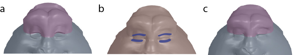
Figure 10. Without saliency weights optimization sometimes fails to produce stop motion results that close the eyes (a). Saliency weights are increased around eyelids (b) to have eyes properly close (c).

Object Velocity

The velocity term (see Equation 3, 4) is critical in preserving the smoothnes and correct timing of transitions between the object in the input. This is especially evident when the library size is much smaller than the number of frames being approximated. Absence of this term can result in both spatial popping (see Figure 11) and temporal sliding (see Figure 12).

Figure 11 illustrates a character gradually opening his mouth. Given a replacement library of two pieces (closed and open mouth), our approach would correctly label the animation, while without the velocity term, we may see short glitches, where the label snaps to an open mouth creating an undesired popping effect.

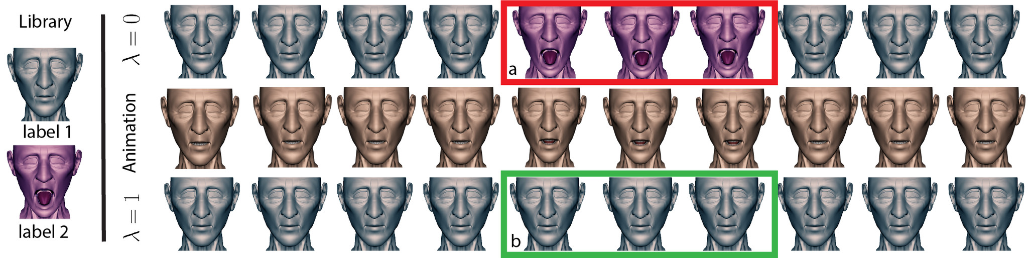
Figure 11. A mouth opening animation (middle) is approximated using 2 pieces. Without the velocity term (top) the few frames (a) where the character slowly opens his mouth are labeled with the extreme open mouth, resulting in a popping artifact. Including the velocity term (bottom) prevents the popping (b).

Figure  12 shows a sudden open mouthed moment of surprise animation. Without the velocity term, both the emotional onset and spatial apex of the input mesh-animation sequence is lost, i.e. the mouth opens earlier than it should and wider, whereas this is preserved with our approach.

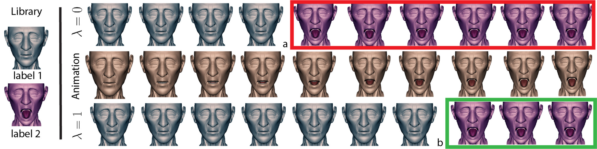
Figure 12. An open-mouthed surprise animation (middle) is approximated using 2 pieces. The replacement and labeling without velocity term (top) snaps the face to an open mouthed surprise too early (a). Including the velocity term (bottom) better preserves the emotional timing (b) of the original animation.

3.4. Part Assembly

Our part segmentation algorithm in Section 3.1 does not guarantee that the object can be physically re-assembled [Luo et al., 2012] and we do not implement any way of holding parts together. Fortunately, in our experiments, the segmentation step has always produced parts that could be assembled after printing. Along the boundaries, the assemblability is locally guaranteed since the gradient condition in Eq. 6 ensures that the normal along the segmentation boundary varies consistently. Global assemblability (see, e.g., [Song et al., 2012]), though not an issue for our examples, could be an interesting avenue for future research. Most studios design custom rigs to hold stop motion parts together in order to ensure that they can be quickly and sturdily swapped out on set. For example, Laika uses magnets slotted into parts which enable animators to quickly swap different parts during the filming process. Rather than assume a particular rig type, we did not focus on the generation of connectors between parts. To realize our experiments, we simply created male/female plugs on parts that connect; these plugs can be fused with the part and 3D printed (see Figure 13).

where the gradient condition not only ensures a unique solution, but also forces the normal of the resulting meshes to vary consistently. This condition is of practical importance for final fabrication: each part can be extruded inward along its normal direction to create a boundary-matching volumetric (printable) shell.

In practice, we implement this for our discrete triangle meshes using the mixed Finite-Element method [Jacobson et al., 2010] (i.e., squared cotangent Laplacian). We implement the gradient condition by fixing one-ring of vertex neighbors along the seams to their average values as well.

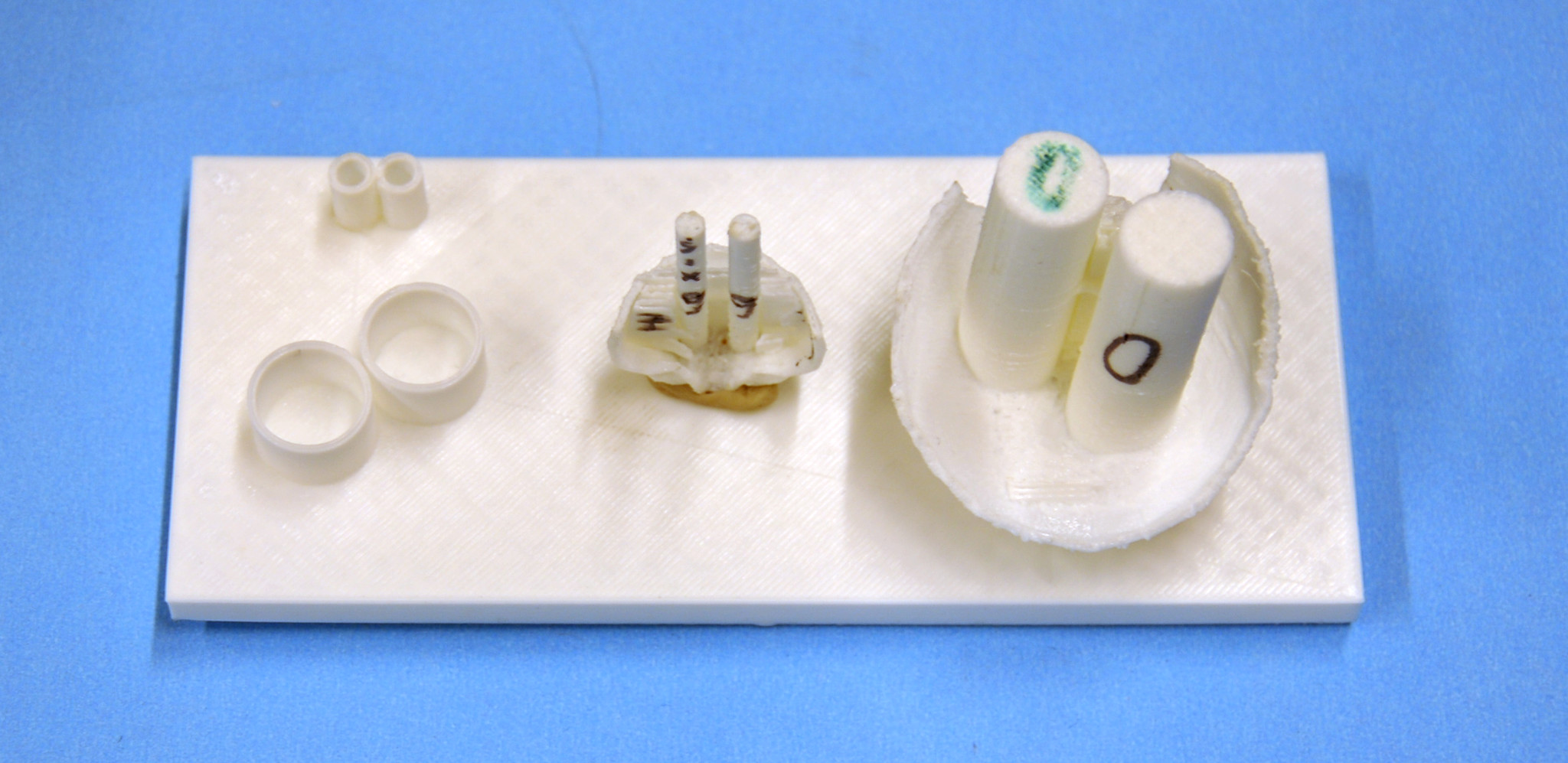
Figure 13. We create male/female plugs to connect the 3D printed “jigs”.

4. Implementation

Our system has been implemented as an integrated standalone application. The algorithms described in Section 3 were implemented in C++ using Eigen [Guennebaud et al., 2010] and libigl [Jacobson et al., 2017]. Our optimization relies on a random seed. We run multiple instances, choosing the best. Each instance takes roughly 5-10 iterations. The entire optimization usually takes around 15-20 seconds for short clips of up $1000$ frames (Table  1). Perfomance was measured on a computer with Interl Xeon CPU @ 2.40GHZ, Nvidia GTX1080 and 64GB of RAM.

The digital library of parts generated using our method was 3D printed with the DREMEL 3D20 3D printer using white PLA material. We manually colored some parts with water based markers. Using a color powder 3D printer will certainly improve the rendered appearance of our results (see Figure 14).

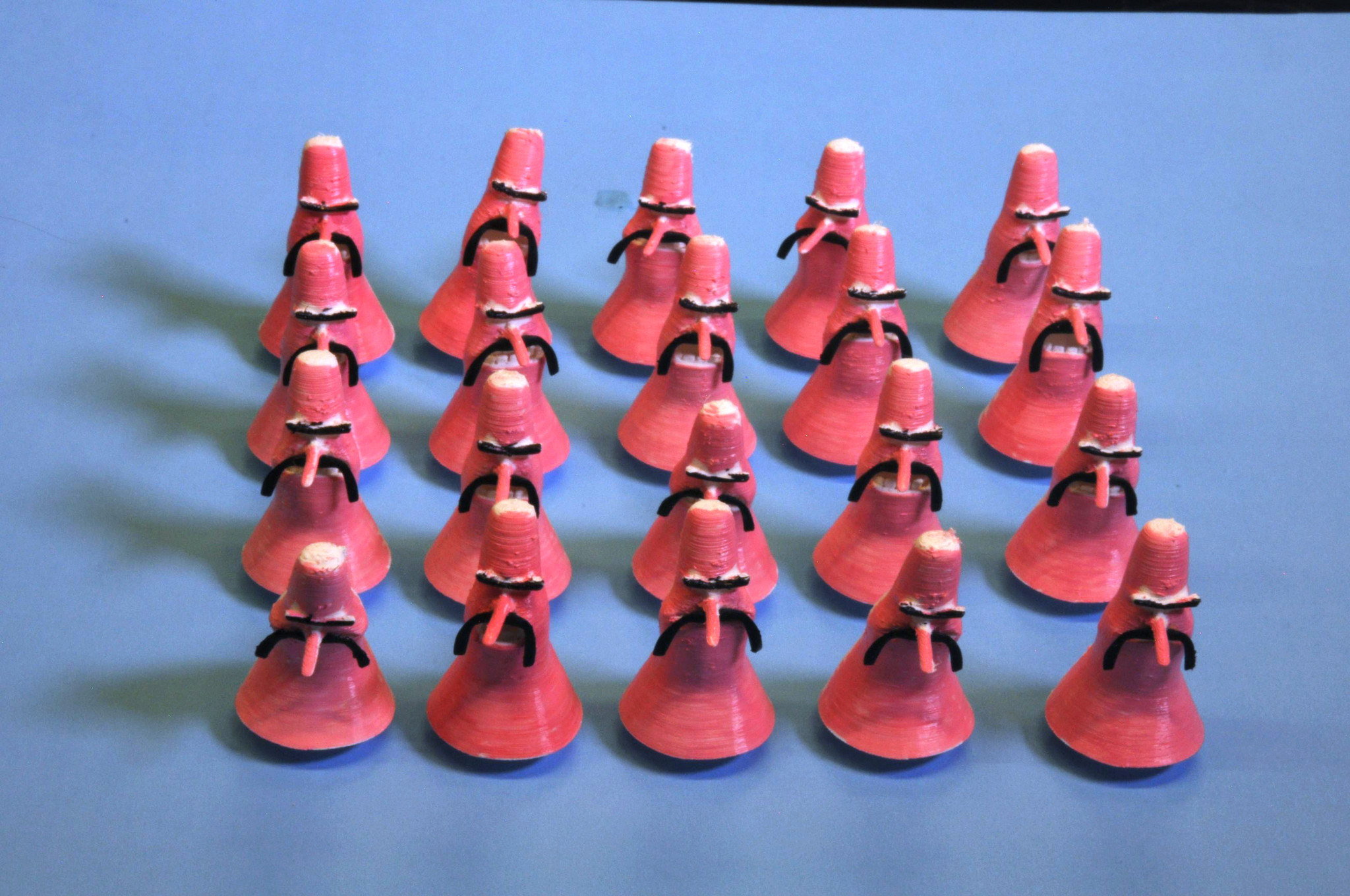
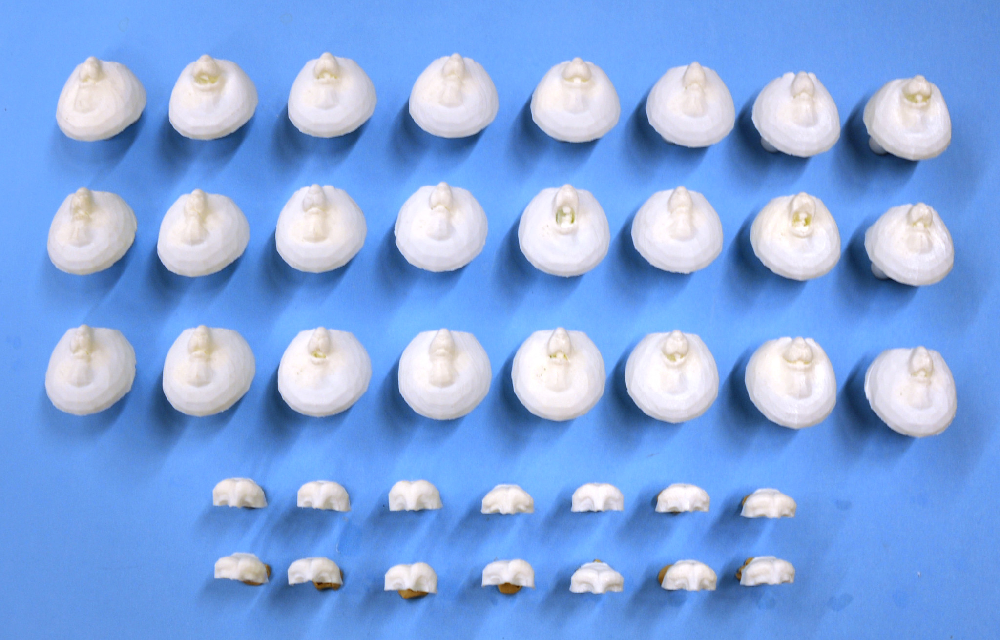
Figure 14. For our physically realized results, we generated 20 cartoon characters and 25 lower bunny faces and 15 upper halves.

Each printed piece is assigned a unique ID and for every frame of the input animations we assign the part IDs mapped by our method in Section 3. The pieces are connected using simple connectors or magnets (Figure 13). We use a Nikon D90 DLSR camera that is controlled by Stop Motion Pro Eclipse software, to view the scene, capture still images and mix stored frames with the live view (see Figure 15). Maintaining precise lighting across sequentially shot frames can be challenging in a research lab and this is evident in our stop-motion clips in the accompanying video.

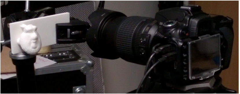
Figure 15. We recreate a typical low-budget stop motion camera setup.

5. Results and Discussion

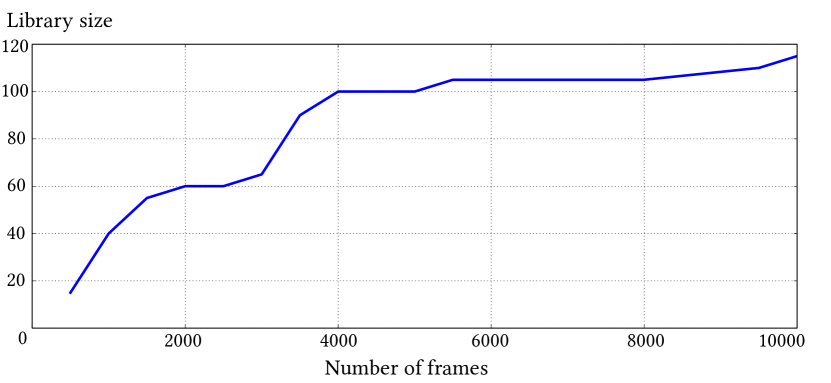
Figure 16. Number of pieces needed to be 3D printed in order to achieve a maximum error threshold per frame.

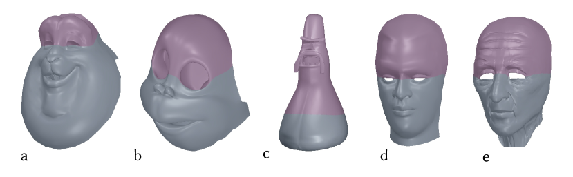
Figure 17. Our method works on cartoon characters (a, b, c) as well as high-fidelity computer animation models (d, e).

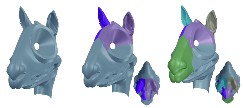
Figure 18. We demonstrate the generality of our system with 3 (middle) and 6 (right) parts segmentation of the input model (left).

Figures 17 and 18 show a variety of faces we animated using our approach (see accompanying video). Even for a single short animation clip, we are able to capture $\approx 750$ frames using two replacement libraries (20+30 pieces), a $25x$ saving over printing each frame. Increasing the number of parts allows to achieve comparable results while decreasing the number of pieces per part. Smaller libraries require less material leading to large cost savings and shorter printing times. For example, given the same budget of 25 pieces per part, we are able to achieve better results with the 6 parts segmentation than the 3 part segmentation or no segmentation at all (Figure  18).

We informally evaluated our approach with a professional animator, who liked the ability to explore the trade-off between animation quality and replacement library size, and felt the method captured the emotional range of the characters well, even for small libraries.

Model	Verticies	Frames	Labels	Time
Monkey	9585	2653	150	39
Bunny	11595	5177	200	152
Oldman	21484	260	20	1
Blobby	60464	229	20	4

Table 1. Perfomance statistics. Time (in seconds) includes labeling and update steps times described in Section 3.3.

We compare our replacement pieces selection and mapping algorithm in Section 3.2 to naive uniform downsampling. Quantitatively, for a 750 frame animation captured using 20 replacement pieces, the overall error for both uniform sampling and our velocity independent ($\lambda=0$) approach is significantly higher than the velocity aware ($\lambda>0$) approach (see Figure 19). While the error in object shape in Figure 19a is comparable or marginally worse for our velocity aware over velocity independent approach, as illustrated in Section 3.2, the velocity error for $\lambda=0$ case in Figure 19b is understandably large. Qualitatively, Figures 11, 12 show the velocity term to be critical to both the selection and mapping to replacement pieces.

Printing time and cost can be prohibitive if the size of the library increases linearly with the number of frames of animation [Priebe, 2011]. In Figure  16, we calculate number of replacement pieces needed in order to stay below a certain per frame error threshold, for 10,000 frames of an animated face reading chapters from the book Moby Dick. Given the labeling and a number of frames, we compute the minimum error value of the sum of the unary and binary terms (Eq.  15,  16) across every frame. We increase the number of replacement parts until the maximum allowed error value is reached. As seen in the figure, the number of replacement parts increases rapidly (from 2 to 100) for 5000 frames or less. However, an additional 5000 frames only leads to a small increase in dictionary size (from 100 to 115), affirming that a reasonably small number of replacement heads can capture the entire expressive range of a character.

Limitations

Our system is the first to address the technical problems of a stop-motion animation workflow and has limitations, subject to future work:

• Our segmentation approach does not respect the aesthetics of a part boundary. While our approach seamlessly connects different parts, the deformation albeit minimal, can adversely impact geometric detail near the part boundary.

• Despite a seamless digital connection, seams between physically printed parts remain visible. Commerical animations often remove these seams digitally by image processing, but film directors like Charlie Kaufman have also made these seams part of the character aesthetic [Murphy, 2015].

• Physically re-assembling the object for every frame sequentially from a large replacement library of pieces can still be cumbersome. This could be addressed by a scheduling algorithm that proposes an order in which to shoot animation frames that minimizes object re-assembly.

• Our replacement part algorithm results are based on vertex position or deformation space distance metrics. We believe our results could be better using a perceptually based distance metric between instances of a deformable object.

• Currently our segmentation algorithm does not explicitly enforce symmetry. Symmetry may sometimes be a desirable property that could be incorporated. However, breaking symmetry has its advantages: the tuft of hair on the Camel’s head in Fig. 18 is assigned to a single — albeit symmetry-breaking — part.

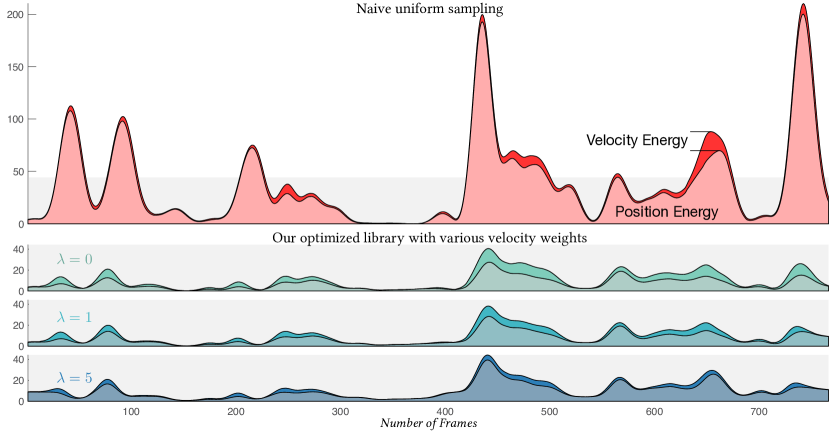
Figure 19. Top: for comparison, we fix the library to a uniform sampling of the deforming object over time (and then use our assignment optimization). Uniform sampling produces very high position error (desaturated area) and high velocity error (saturated area). For visualization, we smooth temporally with a small windowed Gaussian. Below: our optimized library produces dramatically lower error (vertical axis cropped to small gray box). Increasing the velocity weight $λ$ intuitively trades geometric velocity error for position error.

6. Conclusion

Stop-motion animation is a traditional art-form that has seen a surge of popularity with the advent of 3D printing. Our system is the first attempt at an end-to-end solution to the research problems in the creation of stop-motion animations using computer animation and 3D printing. We hope this paper will stimulate new research on the many problems encountered in the area of stop-motion animation.

7. Acknowledgements

This work is funded in part by NSERC Discovery, the Canada Research Chairs Program, Fields Institute CQAM Labs, and gifts from Autodesk, Adobe, and MESH. We thank members of the dgp at University of Toronto for discussions and draft reviews.

References

- [1]
- Alexa and Müller [2000] Marc Alexa and Wolfgang Müller. 2000. Representing Animations by Principal Components. Comput. Graph. Forum (2000).
- Alger et al. [2012] Jed Alger, Travis Knight, and Chris Butler. 2012. The art and making of ParaNorman. Chronicle Books.
- Bäecher et al. [2016] Moritz Bäecher, Benjamin Hepp, Fabrizio Pece, Paul G. Kry, Bernd Bickel, Bernhard Thomaszewski, and Otmar Hilliges. 2016. DefSense: Computational Design of Customized Deformable Input Devices. In SIGCHI.
- Barnes et al. [2008] Connelly Barnes, David E. Jacobs, Jason Sanders, Dan B Goldman, Szymon Rusinkiewicz, Adam Finkelstein, and Maneesh Agrawala. 2008. Video Puppetry: A Performative Interface for Cutout Animation. ACM Trans. Graph. (2008).
- Bergou et al. [2007] Miklós Bergou, Saurabh Mathur, Max Wardetzky, and Eitan Grinspun. 2007. TRACKS: Toward Directable Thin Shells. ACM Trans. Graph. (2007).
- Bickel et al. [2012] Bernd Bickel, Peter Kaufmann, Mélina Skouras, Bernhard Thomaszewski, Derek Bradley, Thabo Beeler, Phil Jackson, Steve Marschner, Wojciech Matusik, and Markus Gross. 2012. Physical face cloning. ACM Transactions on Graphics (TOG) 31, 4 (2012), 118.
- Bonanni and Ishii [2009] Leonardo Bonanni and Hiroshi Ishii. 2009. Stop-motion prototyping for tangible interfaces. Tangible and Embedded Interaction (2009).
- Boykov and Kolmogorov [2004] Yuri Boykov and Vladimir Kolmogorov. 2004. An experimental comparison of min-cut/max-flow algorithms for energy minimization in vision. IEEE transactions on pattern analysis and machine intelligence 26, 9 (2004), 1124–1137.
- Brostow and Essa [2001] Gabriel J. Brostow and Irfan Essa. 2001. Image-based Motion Blur for Stop Motion Animation. In ACM SIGGRAPH.
- Coleman et al. [2008] Patrick Coleman, Jacobo Bibliowicz, Karan Singh, and Michael Gleicher. 2008. Staggered Poses: A Character Motion Representation for Detail-preserving Editing of Pose and Coordinated Timing. In Proc. SCA.
- Didyk et al. [2010] Piotr Didyk, Elmar Eisemann, Tobias Ritschel, Karol Myszkowski, and Hans-Peter Seidel. 2010. Perceptually-motivated Real-time Temporal Upsampling of 3D Content for High-refresh-rate Displays. Comput. Graph. Forum (2010).
- Dvorožnák et al. [2018] Marek Dvorožnák, Wilmot Li, Vladimir G Kim, and Daniel Sỳkora. 2018. Toonsynth: example-based synthesis of hand-colored cartoon animations. ACM Transactions on Graphics (TOG) 37, 4 (2018), 167.
- Edwards et al. [2016] Pif Edwards, Chris Landreth, Eugene Fiume, and K Singh. 2016. JALI: an animator-centric viseme model for expressive lip synchronization. ACM Trans. Graph. (2016).
- Elad and Aharon [2006] Michael Elad and Michal Aharon. 2006. Image denoising via sparse and redundant representations over learned dictionaries. IEEE Transactions on Image processing 15, 12 (2006), 3736–3745.
- Fišer et al. [2017] Jakub Fišer, Ondřej Jamriška, David Simons, Eli Shechtman, Jingwan Lu, Paul Asente, Michal Lukáč, and Daniel Sỳkora. 2017. Example-based synthesis of stylized facial animations. ACM Transactions on Graphics (TOG) 36, 4 (2017), 155.
- Ghosh et al. [2012] Soumya Ghosh, Erik B Sudderth, Matthew Loper, and Michael J Black. 2012. From Deformations to Parts - Motion-based Segmentation of 3D Objects. NIPS (2012).
- Gu et al. [2009] Qin Gu, Jingliang Peng, and Zhigang Deng. 2009. Compression of Human Motion Capture Data Using Motion Pattern Indexing. Computer Graphics Forum (2009).
- Guennebaud et al. [2010] Gaël Guennebaud, Benoît Jacob, et al. 2010. Eigen v3. (2010). http://eigen.tuxfamily.org.
- Han et al. [2014] Xiaoguang Han, Hongbo Fu, Hanlin Zheng, Ligang Liu, and Jue Wang. 2014. A Video-Based System for Hand-Driven Stop-Motion Animation. IEEE CG&A (2014).
- Herholz et al. [2015] Philipp Herholz, Wojciech Matusik, and Marc Alexa. 2015. Approximating Free-form Geometry with Height Fields for Manufacturing. Comput. Graph. Forum 34, 2 (May 2015), 239–251. https://doi.org/10.1111/cgf.12556
- Hu et al. [2014] Ruizhen Hu, Honghua Li, Hao Zhang, and Daniel Cohen-Or. 2014. Approximate Pyramidal Shape Decomposition. ACM Trans. Graph. 33, 6, Article 213 (Nov. 2014), 12 pages. https://doi.org/10.1145/2661229.2661244
- Jacobson et al. [2017] Alec Jacobson, Daniele Panozzo, et al. 2017. libigl: A simple C++ geometry processing library. (2017). http://libigl.github.io/libigl/.
- Jacobson et al. [2010] Alec Jacobson, Elif Tosun, Olga Sorkine, and Denis Zorin. 2010. Mixed Finite Elements for Variational Surface Modeling.
- James and Twigg [2005] Doug L. James and Christopher D. Twigg. 2005. Skinning Mesh Animations. ACM Trans. Graph. 24, 3 (July 2005), 399–407.
- Jeong and Sim [2014] Se-Won Jeong and Jae-Young Sim. 2014. Multiscale saliency detection for 3D meshes using random walk. APSIPA (2014).
- Knep et al. [1995] Brian Knep, Craig Hayes, Rick Sayre, and Tom Williams. 1995. Dinosaur Input Device. In Proc. CHI. 304–309.
- Kolevsohn [2009] Lynn Kolevsohn. 2009. Objet Geometries’ 3-D Printers Play Starring Role in New Animated Film Coraline. http://www.prnewswire.co.uk/news-releases/objet-geometries-3-d-printers-play-starring-role-in-new-animated-film-coraline-155479455.html (2009).
- Kolmogorov and Zabin [2004] Vladimir Kolmogorov and Ramin Zabin. 2004. What energy functions can be minimized via graph cuts? IEEE TPAMI (2004).
- Kyprianidis et al. [2013] Jan Eric Kyprianidis, John Collomosse, Tinghuai Wang, and Tobias Isenberg. 2013. State of the "Art”: A Taxonomy of Artistic Stylization Techniques for Images and Video. IEEE Transactions on Visualization and Computer Graphics 19, 5 (May 2013), 866–885. https://doi.org/10.1109/TVCG.2012.160
- Le and Deng [2013] Binh Huy Le and Zhigang Deng. 2013. Two-layer sparse compression of dense-weight blend skinning. ACM Transactions on Graphics (2013).
- Le and Deng [2014] Binh Huy Le and Zhigang Deng. 2014. Robust and accurate skeletal rigging from mesh sequences. ACM Trans. Graph. (2014).
- Lee et al. [2006] Tong-Yee Lee, Yu-Shuen Wang, and Tai-Guang Chen. 2006. Segmenting a deforming mesh into near-rigid components. The Visual Computer 22, 9-11 (2006), 729–739.
- Lewis et al. [2014] John P Lewis, Ken Anjyo, Taehyun Rhee, Mengjie Zhang, Frédéric H Pighin, and Zhigang Deng. 2014. Practice and Theory of Blendshape Facial Models. Eurographics (2014).
- Lloyd [1982] Stuart P. Lloyd. 1982. Least squares quantization in pcm. IEEE Transactions on Information Theory 28 (1982), 129–137.
- Luo et al. [2012] Linjie Luo, Ilya Baran, Szymon Rusinkiewicz, and Wojciech Matusik. 2012. Chopper: Partitioning Models into 3D-printable Parts. ACM Trans. Graph. (2012).
- Murphy [2015] Mekado Murphy. 2015. Showing the Seams in ‘Anomalisa’. https://www.nytimes.com/interactive/2015/12/18/movies/anomalisa-behind-the-scenes.html (2015).
- Neumann et al. [2013] Thomas Neumann, Kiran Varanasi, Stephan Wenger, Markus Wacker, Marcus A Magnor, and Christian Theobalt. 2013. Sparse localized deformation components. ACM Trans. Graph. (2013).
- Noh and Igarashi [2017] Seung-Tak Noh and Takeo Igarashi. 2017. Retouch Transfer for 3D Printed Face Replica with Automatic Alignment. In Proc. CGI.
- Otani et al. [2016] Mayu Otani, Yuta Nakashima, Esa Rahtu, Janne Heikkilä, and Naokazu Yokoya. 2016. Video Summarization Using Deep Semantic Features. In Asian Conference on Computer Vision.
- Priebe [2011] Kenneth A Priebe. 2011. The advanced art of stop-motion animation. Cengage Learning.
- Ribera et al. [2017] Roger Ribera, Eduard Zell, J. P. Lewis, Junyong Noh, and Mario Botsch. 2017. Facial Retargeting with Automatic Range of Motion Alignment. ACM Trans. Graph. (2017).
- Sattler et al. [2005] Mirko Sattler, Ralf Sarlette, and Reinhard Klein. 2005. Simple and Efficient Compression of Animation Sequences. In SCA. ACM, New York, NY, USA, 209–217.
- Seo et al. [2011] Jaewoo Seo, Geoffrey Irving, J P Lewis, and Junyong Noh. 2011. Compression and direct manipulation of complex blendshape models. ACM Trans. Graph. (2011).
- Shamir [2008] Ariel Shamir. 2008. A survey on Mesh Segmentation Techniques. Comput. Graph. Forum (2008).
- Singh and Fiume [1998] Karan Singh and Eugene Fiume. 1998. Wires: A Geometric Deformation Technique. In ACM SIGGRAPH.
- Song et al. [2012] Peng Song, Chi-Wing Fu, and Daniel Cohen-Or. 2012. Recursive interlocking puzzles. ACM Transactions on Graphics (TOG) 31, 6 (2012), 128.
- Vasa et al. [2014] L. Vasa, S. Marras, K. Hormann, and G. Brunnett. 2014. Compressing dynamic meshes with geometric laplacians. Computer Graphics Forum 33, 2 (2014), 145–154.
- Wang et al. [2004] Jue Wang, Yingqing Xu, Heung-Yeung Shum, and Michael F. Cohen. 2004. Video Tooning. In ACM SIGGRAPH.
- Wang et al. [2016] W. M. Wang, C. Zanni, and L. Kobbelt. 2016. Improved Surface Quality in 3D Printing by Optimizing the Printing Direction. In Proceedings of the 37th Annual Conference of the European Association for Computer Graphics (EG ’16). Eurographics Association, Goslar Germany, Germany, 59–70. https://doi.org/10.1111/cgf.12811
- Whited et al. [2010] Brian Whited, Gioacchino Noris, Maryann Simmons, Robert W Sumner, Markus H Gross, and Jarek Rossignac. 2010. BetweenIT - An Interactive Tool for Tight Inbetweening. Comput. Graph. Forum (2010).
- Witkin and Kass [1988] Andrew P Witkin and Michael Kass. 1988. Spacetime constraints. Siggraph (1988).
- Wright et al. [2010] John Wright, Yi Ma, Julien Mairal, Guillermo Sapiro, Thomas S Huang, and Shuicheng Yan. 2010. Sparse representation for computer vision and pattern recognition. Proc. IEEE 98, 6 (2010), 1031–1044.
- Y. Boykov et al. [2001] Y Y. Boykov, O Veksler R., and R Zabih. 2001. Efficient Approximate Energy Minimization via Graph Cuts. 20 (01 2001).
- Zhang et al. [2015] Xiaoting Zhang, Xinyi Le, Athina Panotopoulou, Emily Whiting, and Charlie C. L. Wang. 2015. Perceptual Models of Preference in 3D Printing Direction. ACM Trans. Graph. (2015).