Efficient Detection and Quantification of Timing Leaks with Neural Networks

Abstract

Detection and quantification of information leaks through timing side channels are important to guarantee confidentiality. Although static analysis remains the prevalent approach for detecting timing side channels, it is computationally challenging for real-world applications. In addition, the detection techniques are usually restricted to “yes” or “no” answers. In practice, real-world applications may need to leak information about the secret. Therefore, quantification techniques are necessary to evaluate the resulting threats of information leaks. Since both problems are very difficult or impossible for static analysis techniques, we propose a dynamic analysis method. Our novel approach is to split the problem into two tasks. First, we learn a timing model of the program as a neural network. Second, we analyze the neural network to quantify information leaks. As demonstrated in our experiments, both of these tasks are feasible in practice — making the approach a significant improvement over the state-of-the-art side channel detectors and quantifiers. Our key technical contributions are (a) a neural network architecture that enables side channel discovery and (b) an MILP-based algorithm to estimate the side-channel strength. On a set of micro-benchmarks and real-world applications, we show that neural network models learn timing behaviors of programs with thousands of methods. We also show that neural networks with thousands of neurons can be efficiently analyzed to detect and quantify information leaks through timing side channels.

1 Introduction

Programs often handle sensitive data such as credit card numbers or medical histories. Developers are careful that eavesdroppers cannot easily access the secrets (for instance, by using encryption algorithms). However, a side channel might arise even if the transferred data is encrypted. For example, in timing side channels [12], an eavesdropper who observes the response time of a server might be able to infer the secret input, or at least significantly reduce the remaining entropy of possible secret values. Studies show that side-channel attacks are practical [30, 14, 27].

Detecting timing side channels are difficult problems for static analysis, especially in real-world Java applications. From the theoretical point of view, side-channel presence cannot be inferred from one execution trace, but rather, an analysis of equivalence classes of traces is needed [43]. From a practical perspective, the problem is hard because timing is not explicitly visible in the code. A side channel is a property of the code and the platform on which the program is executed. In addition, most existing static techniques rely on taint analysis that is computationally difficult for applications with dynamic features [33].

A large body of work addresses the problem of detecting timing side channels [13, 41, 5]. However, detection approaches are often restricted to either “yes” or “no” answers. In practice, real-world applications may need to leak information about the secret [44]. Then, it is important to know “how much” information is being leaked to evaluate the resulting threats. Quantification techniques with entropy-based measures are the primary tools to calculate the amount of leaks.

We propose a data-driven dynamic analysis for detecting and quantifying timing leaks. Our approach is to split the problem into two tasks: first, to learn a timing model of the program as the neural network (NN) and second, to analyze the NN, which is a simpler object than the original program. The key insight that we exploit is that timing models of the program are easier to learn than the full functionality of the program. The advantages of this approach are two-fold. First, although general verification problems are difficult in theory and practice, learning the timing models is efficiently feasible, as shown in our experiments. We conjecture that this is because timing behaviors reflect the computational complexity of a program, which is usually a simpler function of the input rather than the program. Second, neural networks, especially with ReLU units, are easier models to analyze than programs.

Our key technical ideas are enabling a side channel analysis using a specialized neural network architecture and a mixed integer linear programming (MILP) algorithm to estimate an entropy-based measure of side-channel strengths. First, our NN consists of three parts: (a) encoding the secret inputs, (b) encoding the public inputs, and (c) combining the outputs of the first two parts to produce the program timing model. This architecture has the advantage that we can easily change the “strength” (the number of neurons $k$) of the connection from the secret inputs. This enables us to determine whether there is a side channel. If timing can not be accurately predicted based on just public inputs ($k{=}0$), then there is a timing side channel. Second, for $k{>}0$, the trained NN can be analyzed to estimate the strength of side-channel leaks. Each valuation of the $k$ binarized output of secret part corresponds to one observationally distinguishable class of secret values. We use an MILP encoding to estimate the size of classes and calculate the amount of information leaks with entropy-based objectives such as Shannon entropy.

Our empirical evaluation shows both that timing models of programs can be represented as neural networks and that these NNs can be analyzed to discover side channels and their strengths. We implemented our techniques using Tensorflow [2] and Gurobi [25] for learning timing models as NN objects and analyzing the NNs with MILP algorithms, respectively. We ran experiments on a Linux machine with 24 cores of 2.5 GHz. We could learn timing model of programs (relevant to the observed traces) with few thousands methods in less than 10 minutes with the accuracy of 0.985. Our analysis can handle NN models with thousands of neurons and retrieve the number of solutions for each class of observation. The number of solutions enables us to quantify the amount of information leaks.

In summary, our key contributions are:

• An approach for side channel analysis based on learning execution times of a program as a NN.

• A tunable specialized NN architecture for timing side-channel analysis.

• An MILP-based algorithm for estimating entropy-based measures of information leaks over the NN.

• An empirical evaluation that shows our approach is scalable and quantifies leaks for real-world Java applications.

2 Overview

We illustrate on examples the key ingredients of our approach: learning timing models of programs using neural networks and a NN architecture that enables us to detect and quantify timing leaks.

Learning timing models of programs. Learning the functionality of the sorting algorithms from programs is difficult, while learning their timing model is much easier. We picked the domain of sorting algorithms as these algorithms have well-known different timing behaviors. We implement six different sorting algorithms namely bubble sort, selection sort, insertion sort, bucketing sort, merging sort, and quick sort in one sorting application. We generate random arrays of different sizes from 100 to 20,000 elements and run the application for each input array with different sorting algorithms. This implies that we consider the average-case computational complexities of different algorithms. Each data point consists of the input array, the indicator of sorting algorithm, and the execution time of sorting application. In addition, the data points are independent from each other, and the neural network learns end-to-end execution times of the entire application, not individual sorting algorithms. Figure 1 (a) shows the learned execution times for the sorting application. The neural network model has 6 layers with 825 neurons. The accuracy of learning based on coefficient of determination ($R^{2}$) over test data is 0.999, and the learning takes 308.7 seconds (the learning rate is 0.01). As we discussed earlier, the NN model predicts (approximates) execution times for the whole sorting application. Further analysis is required to decompose the NN model for individual sorting algorithms that is not relevant in our setting since we are only interested in learning end-to-end execution times of applications. Using the neural network model to estimate execution times has two important advantages over the state-of-the-art techniques [23, 50]. First, the neural network can approximate an arbitrary timing model as a function of input features, while the previous techniques can only approximate linear or polynomial functions. Second, the neural network does not require feature engineering, whereas the previous techniques require users to specify important input features such as work-load (size) features.

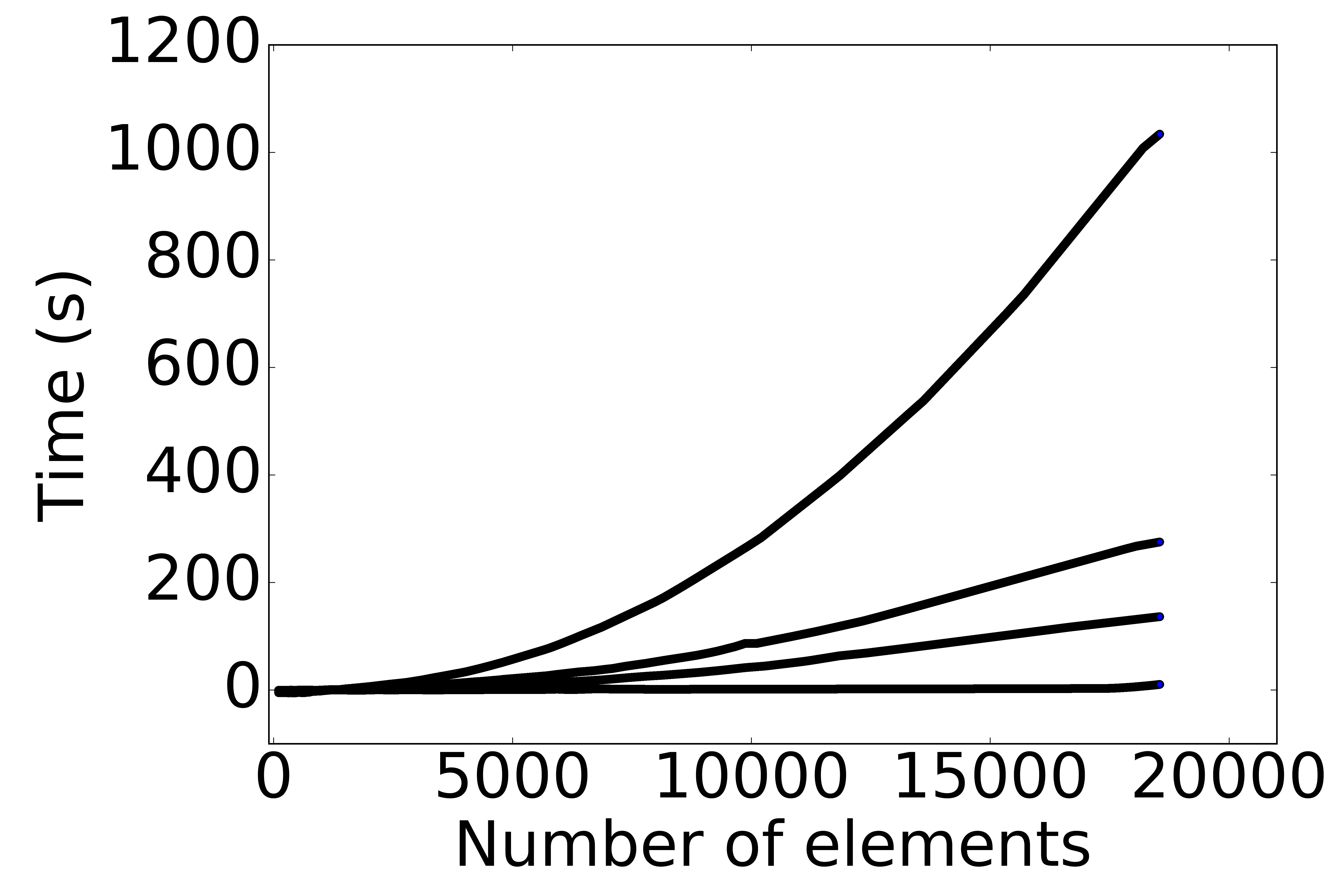
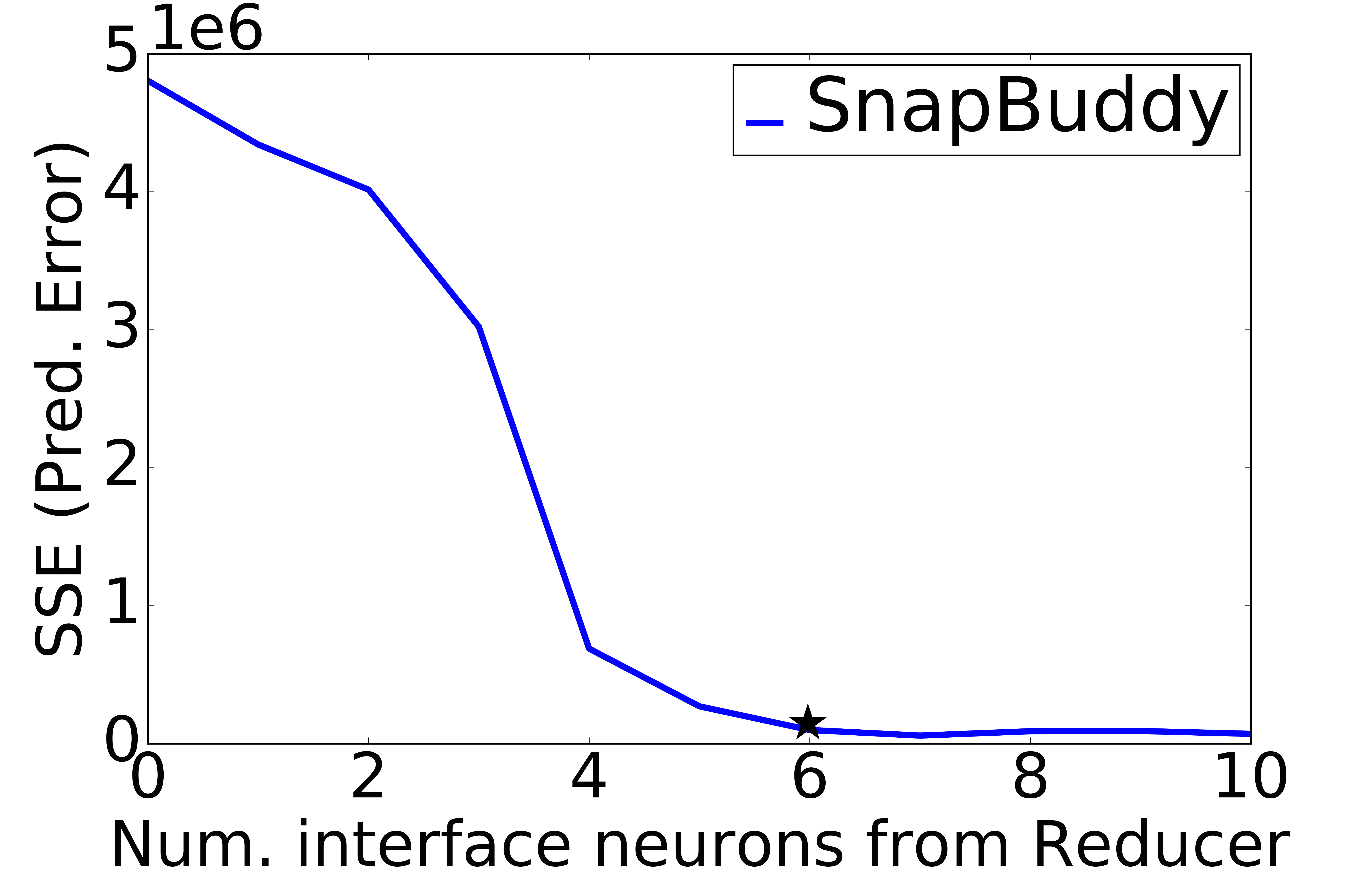
Figure 1: (a) Timing models of the sorting application as learned by NNs. (b) Prediction error vs. the number of neurons ($k$) in the interface layer of SnapBuddy.

Neural network architecture for side channel discovery. With the observations that the neural networks can learn programs’ execution times precisely, we consider a special architecture to analyze timing side channels of programs. We propose the neural network architecture shown in Figure 2. The NN architecture consists of three parts: 1) A reducer function that learns a map from $n$ secret features (inputs) to $k$ binarized interface neurons (we call them interface neurons as they connect the secret inputs to the rest of the network); 2) A neural network function that connects the public features to the overall model; 3) A joint function that uses the output of the reducer and public-features functions to predict the execution times. The architecture makes it easy to change the number of neurons ($k$) in the connection from the reducer, which enables us to estimate the side-channel strength. In this architecture, there are timing side channels if the value for $k$ is greater than or equal to 1. The NN learning is to find the weights in different layers with the optimal number of neurons in the interface layer ($k$) such that the NN approximates execution times accurately.

Estimating the side channel strength. The side-channel strength is estimated by finding the minimal value of $k$ in the learning of accurate NN models. We use Sum of Squared Error (SSE) measure to compute prediction errors. Figure 1 (b) shows the SSE versus the number of interface neurons ($k$) for the SnapBuddy application (described in Section 6.2). As shown in the plot, the prediction error decreases as the number of neurons increase from 0 to 6. But, after 6, the prediction error stays almost the same. We thus choose 6 as the optimal number of interface neurons. Since each neuron is a binary unit, there are $2^{6}$ distinct outputs from the reducer function. Each distinct output forms a class of observation over the secret inputs. However, some classes of observations might be empty and are not feasible from any secret value. Furthermore, for feasible classes, the entropy measures require the number of elements in each class. We encode the reducer function as a mixed integer linear programming (MILP) problem. Then, we calculate the number of feasible solutions for each class. For SnapBuddy, it takes 16.6 seconds to analyze the reducer function and find the number of solutions for non-empty classes. Using Shannon entropy, the analysis shows 3.0 bits of information about secret inputs are leaking in SnapBuddy.

Figure 2: Neural network architecture for side-channel discovery and quantification. The NN takes secret features ($\mathbf{x}$) and public features ($\mathbf{y}$), and it learns weights $W$ with the minimal number of neurons in the interface layer ($\mathcal{L}_{\alpha}^{S}$) to precisely predict execution times. The reducer function maps $n$-dimensional $\mathbf{x}$ to $k$ binary outputs. The MILP analysis of reducer function is used for the quantification.

3 Problem Statement

We develop a framework for detecting and quantifying information leaks due to the execution time of programs. Our framework is suitable for known-message and chosen-message threat [32] settings where the variations in the execution times depend on both public and secret inputs.

The timing model $[\![{\mathcal{P}}]\!]$ of a program $\mathcal{P}$ is a tuple $(X,Y,\mathcal{S},\delta)$ where $X{=}\{x_{1},\ldots$ $,x_{n}\}$ is the set of secret input variables, $Y=\left\{y_{1},y_{2},\ldots,y_{m}\right\}$ is the set of public input variables, and $\mathcal{S}\subseteq\mathbb{R}^{n}$ is a finite set of secret inputs, and $\delta:\mathbb{R}^{n}\times\mathbb{R}^{m}\to\mathbb{R}_{\geq 0}$ is the execution-time of the program as a function of secret and public inputs. A timing function of the program $\mathcal{P}$ for a secret input $s\in\mathcal{S}$ is the function $\delta(s)$ defined as $\mathbf{y}\in\mathbb{R}^{m}\mapsto\delta(s,\mathbf{y})$. Let $\mathcal{F}$ be the set of all timing functions in $\mathcal{P}$.

Given a timing model $[\![{\mathcal{P}}]\!]$ and a tolerance $\varepsilon{>}0$, a $k$-bit $\varepsilon$-approximate secret reducer is a pair

$$(\alpha,\beta)\in[\mathbb{R}^{n}\to\mathbb{B}^{k}]\times[\mathbb{B}^{k}\to\mathbb{R}^{n}]$$

such that $\|\delta(\mathbf{x})-\delta(\beta(\alpha(\mathbf{x})))\|\leq\varepsilon$ for every $\mathbf{x}\in\mathcal{S}$ where $\|\cdot\|$ is some fixed norm over the space of timing function. In this paper, we work with $\infty$-norm. We write $R_{(\varepsilon,k)}$ for the set of all $k$-bit $\varepsilon$-approximate reducers for $[\![{\mathcal{P}}]\!]$. We say that $(\alpha,\beta)\in R_{(\varepsilon,k)}$ is an optimal $\varepsilon$-approximate reducer if for all $k^{\prime}<k$ the set $R_{(\varepsilon,k^{\prime})}$ is empty. Given a tolerance $\varepsilon>0$, we say that there are information leaks in execution times, if there is no $0$-bit $\varepsilon$-approximate optimal secret reducer.

A reducer $(\alpha,\beta)$ characterizes an equivalence relation $\equiv_{\alpha}$ over the set of secrets $\mathcal{S}$, defined as the following: $s\equiv_{\alpha}s^{\prime}$ if $\alpha(s)=\alpha(s^{\prime})$. Let $\mathcal{S}_{[\alpha]}=\langle\mathcal{S}_{1},\mathcal{S}_{2},\ldots,\mathcal{S}_{K}\rangle$ be the quotient space of $\mathcal{S}$ characterized by the reducers $(\alpha,\beta)$; note that $2^{k-1}<K\leq 2^{k}$. Let $\mathcal{B}=\langle B_{1},B_{2},\ldots,B_{K}\rangle$ be the size of observational equivalence class in $\mathcal{S}_{\alpha}$, i.e. $B_{i}=|\mathcal{S}_{i}|$ and let $B=|\mathcal{S}|=\sum_{i=1}^{K}B_{i}$. The expected information leaks due to observations on the execution times of a program can be quantified by using the difference between the uncertainty about the secret values before and after the timing observations. Assuming that secret values $\mathcal{S}$ are uniformly distributed, we quantify information leaks [31] as

$$\textsf{SE}(\mathcal{S}|\alpha)\stackrel{{\scriptstyle\mbox{\rm{\tiny def}}}}{{=}}{\log_{2}(B)}-\frac{1}{B}\sum\limits_{i{=}1}^{K}B_{i}\log_{2}(B_{i}).$$ (1)

Given a program with inputs partitioned into secret and public inputs, our goal is to quantify the information leaks through timing side channels. However, such programs often have complex functionality with black-box components. Moreover, the shape of timing functions may be non-linear and unknown. We propose a neural-network architecture to approximate the timing model as well as to quantify information leakage due to the timing side channels in the program. We then analyze this network to precisely quantify the information leaks based on the equation (1).

4 Neural Network Architecture to Detect and Quantify Information Leaks

A rectified linear unit (ReLU) is a function $\sigma:\mathbb{R}\to\mathbb{R}$ defined as $x\mapsto\max\left\{x,0\right\}$. We can generalize this function from scalars to vectors as $\sigma:\mathbb{R}^{n}\to\mathbb{R}^{n}$ in a straightforward fashion by applying ReLU component-wise. In this paper, we primarily work with feedforward neural network (NN) with ReLU activation units. A $\mathbb{R}^{w_{0}}\to\mathbb{R}^{w_{N+1}}$ feedforward neural network $\mathcal{N}$ is characterized by its number of hidden layers (or depth) $N$, the input and output dimensions $w_{0},w_{N+1}\in\mathbb{N}$, and width of its hidden layers $w_{1},w_{2},\ldots,w_{N}$. Each hidden layer $i$ implements an affine mapping $T_{i}:\mathbb{R}^{w_{i-1}}\to\mathbb{R}^{w_{i}}$ corresponding to the weights in each layer. The function $f_{\mathcal{N}}:\mathbb{R}^{w_{0}}\to\mathbb{R}^{w_{N+1}}$ implemented by neural network $\mathcal{N}$ is:

$$f_{\mathcal{N}}=T_{k+1}\circ\sigma\circ T_{k}\circ\sigma\circ\cdots T_{2}\circ\sigma\circ T_{1}.$$

It is well known that NNs with ReLU units implement a piecewise-linear function [8] and due to this property, it can readily be encoded [21] as a mixed integer linear programming (MILP).

Given a target (black-box) function $f:\mathbb{R}^{w_{0}}\to\mathbb{R}^{w_{N+1}}$ to be approximated and a neural network architecture $(w_{0},w_{1},\ldots,w_{N+1})\in\mathbb{R}^{N+2}$, the process of training the network is to search for weights of various layers so as to closely approximate the function $f$ based on noisy approximate examples from the function $f$. The celebrated universal approximation theorems about neural networks state that deep feedforward neural networks [16, 26]—equipped with simple activation units such as rectified linear unit (ReLU)—can approximate arbitrary continuous functions on a compact domain to an arbitrary precision. Assuming that the timing functions of a program have bounded discontinuities, it can be approximated with a continuous function to an arbitrary precision. It then follows that one can approximate the execution-time function to an arbitrary precision using feedforward neural networks.

Figure 3: Neural Network $\mathcal{N}_{\delta}$ approximating the execution-time function $\delta$ along with a reducer $(\mathcal{N}_{\alpha},\mathcal{N}_{\beta})$.

Figure 3 shows different components of our neural network model. We train a neural network $\mathcal{N}_{\delta}:\mathbb{R}^{n+m}\to\mathbb{R}$ (where the input variables are partitioned into secret and public and the output variable is the execution time) to approximate the execution times of a given program to a given precision $\varepsilon>0$. In order to quantify the number of secret bits leaked in the timing functions, we train a pair of $k$-bit reducer neural networks $\mathcal{N}_{\alpha}:\mathbb{R}^{n}\to\mathbb{B}^{k}$ and $\mathcal{N}_{\beta}:\mathbb{B}^{k}\to\mathbb{R}^{n}$ with the output of $\mathcal{N}_{\beta}$ connected to the neural network $\mathcal{N}_{\delta}$. In this training, we only learn the weights of $\mathcal{N}_{\alpha}$ and $\mathcal{N}_{\beta}$ while keeping the weights of $\mathcal{N}_{\delta}$ unchanged. We call the composition of these networks $\mathcal{N}_{k}=\mathcal{N}_{\alpha}\circ\mathcal{N}_{\beta}\circ\mathcal{N}_{\delta}$. It is easy to see that the network pair $(\mathcal{N}_{\alpha},\mathcal{N}_{\beta})$ implements a $k$-bit secret reducer $(f_{\mathcal{N}_{\alpha}},f_{\mathcal{N}_{\beta}})$. Let $k$ be the smallest number such that the fitness of $\mathcal{N}_{k}$ is comparable to the fitness of $\mathcal{N}_{\delta}$. We find the smallest $k\in\mathbb{N}$ such that $\mathcal{N}_{k}$ approximate the execution time as closely as $\mathcal{N}$. The value $k$ characterizes the number of observational classes over the secret inputs in the program and corresponding network $\mathcal{N}_{\alpha}$ characterizes the secret elements in each class of observation.

We use an MILP encoding, similar to [21, 40, 18] but in backward analysis fashions, to count the number of secret elements in each observational class as characterized by the network $\mathcal{N}_{\alpha}$. These counts can then be used to provide a quantitative measure of information leaks in the program due to the execution times. Since the function $\beta$ is not directly useful in quantification process, we use a simpler network model, in our experiments, to compute the reducer function $\alpha$ as shown in Figure 2.

5 Experiments

5.1 Implementations

Environment Setup. All timing measurements from programs are conducted on an NUC5i5RYH machine. We run each experiment multiple times and use the mean of running time for the rest of analysis. We use a super-computing machine for the training and analysis of the neural network. The machine has a Linux Red Hat 7 OS with 24 cores of 2.5 GHz CPU each with 4.8 GB RAM.

Neural Network Learning. The neural network model is implemented using TensorFlow [2]. We randomly choose 10% of the data for testing, and the rest for the training. We use ReLU units as activation functions and apply mini-batch SGD with the Adam optimizer [29] where the learning rate varies from 0.01 to 0.001 for different benchmarks. For the reducer function of our NN model, we binarize the output of every layer using the “straight-through” technique [15] to estimate the activation function in the backward propagation of errors known as backpropagation [35].

Quantification of Information Leaks. After training, we analyze the reducer function using mixed integer linear programming (MILP) [21, 40]. We encode the MILP model in Gurobi [25] and use the PoolSolutions option to retrieve feasible solutions (up to 2 Billions). For each class of observation (each distinct output of interface layer), the Gurobi calculates possible solutions from the secret inputs such that the output value of interface layer is feasible from those inputs. We use the number of solutions for each class and apply Shannon entropy to quantify the amount of information leaks.

5.2 Micro-benchmarks

First, we show our approach for finding the (optimal) number of interface neurons ($k$) from the reducer function. Then, we show the scalability and usefulness of our approach. scalability: We use the size of neural network, computation time for learning, and the computation time for analyzing. usefulness: We consider the number of classes of observations, the fitness of predictions, and entropy measures. We also compare the entropy values to ground truth.

Programs. We use two sets of micro-benchmark programs for our studies. The first one, taken from [50], uses the names R_n where n is the number of secret bits in the program. The benchmarks were constructed to exhibit complex relationships between secret bits that influence the running time. Each relationship is a boolean formula over the secret input where the true evaluation triggers a (linear) loop statement over the public inputs.

For Branch_Loop (B_L) applications [51], the program does different computations with different complexities depending on the values of the secret input. There are four loop complexities: O($\log(N)$), O($N$), O($N.\log(N)$), and O($N^{2}$) where $N$ is the public input. Each micro-benchmark B_L_i has all four loop complexities, and there are $i$ types of each complexity with different constant factors such as O($\log(N)$) and O($2.\log(N)$) for B_L_2.

Optimal number of reducer outputs. Since the number of observational classes of the secret inputs depends on the number of interface neurons ($k$) from the reducer function, we choose the optimal value for k. We consider the sum of squared error (SSE) versus the number of interface neurons (k). We choose a value k such that the SSE error decreases from 0 to k ($k\geq 0$) and stays almost same for larger values of k. Figure 4 (a) and Figure 4 (b) show the plot of the SSE error vs number of interface neurons for R_n and B_L_n, respectively. For example, in B_L_5, the optimal number of interface neurons is 7.

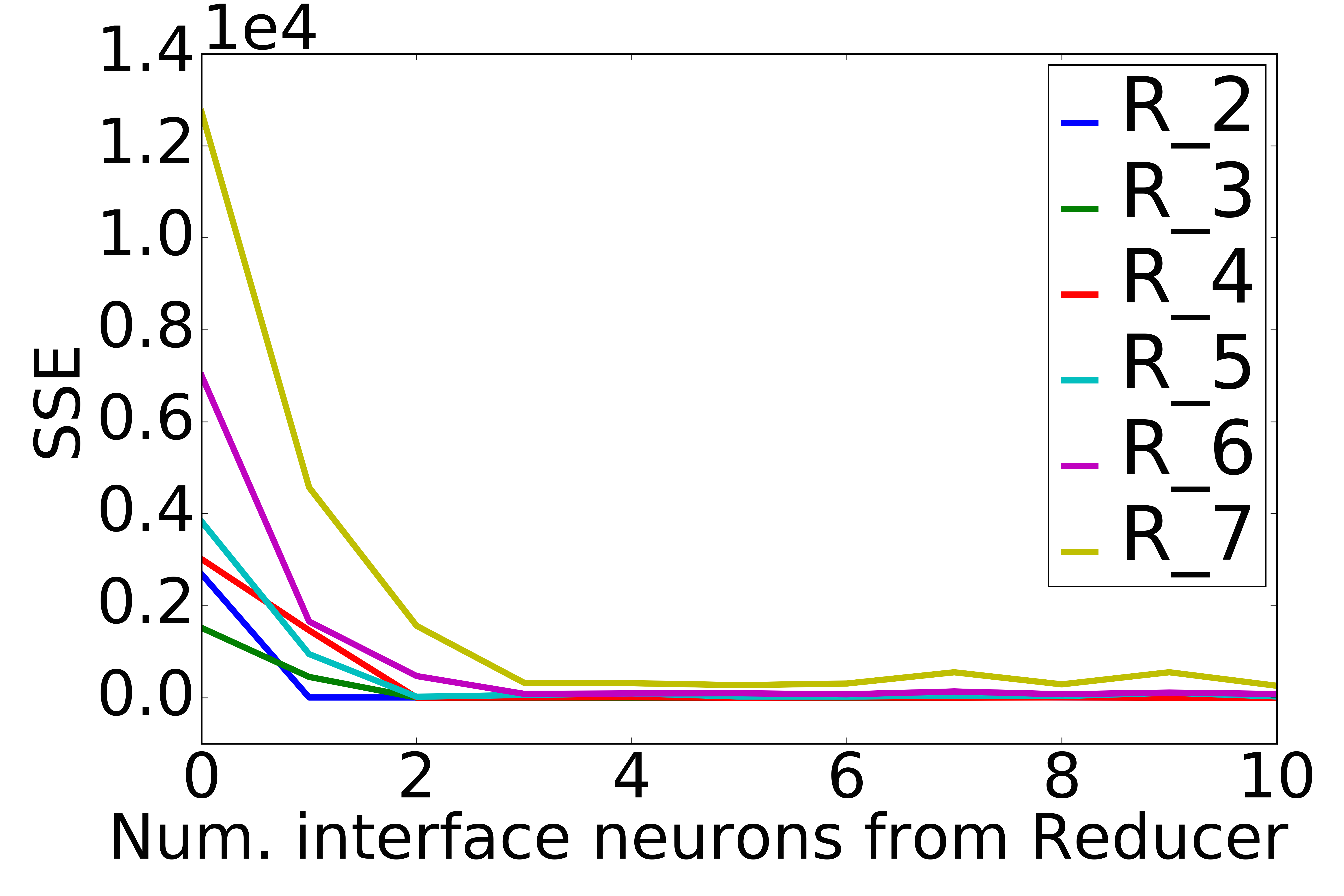
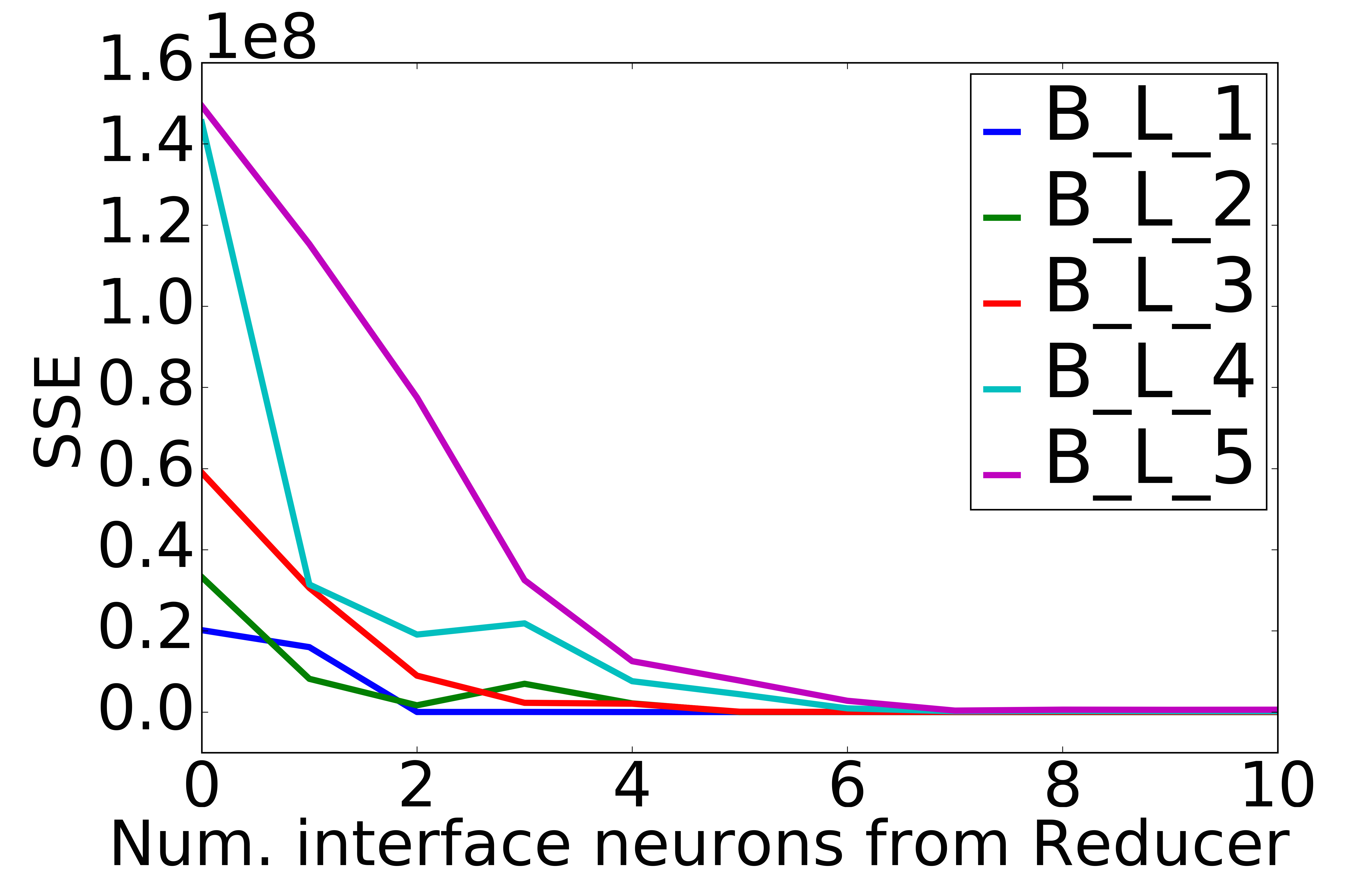
Figure 4: (a) The SSE versus the number of interface neurons for R_n. (b) The SSE versus the number of interface neurons for B_L_n.

Scalability Results. Table 1 shows that our approach is scalable for learning timing models of programs. For example, we could learn the time model of B_L_5 program with the NN model of 7 internal layers and 717 neurons in 25 mins. In addition, the growth in computation times of learning is proportional to the growth in the size of networks. The results show that our approach is scalable for analyzing the reducer function of NN. For this analysis, we only consider the secret parts of NN (shown with $L_{S}$ in Table 1). The computation time for the analysis depends on the size of secret inputs and the size of reducer function. In B_L_5 program with 7 interface neurons of the reducer, we calculate feasible solutions over secret inputs for each $2^{7}$ possible classes. It takes about 8 minutes to analyze the reducer function of B_L_5 program. The growth in the computation times of network analysis is also proportional to the growth in the size of secret inputs and the size of reducer. For example, the computation time for the analysis of B_L_4 example is increased by almost 12 times in comparison to B_L_3, but the size of input, the interface, and the internal neurons have increased by two times (from $2^{11}$ to $2^{12}$), two times (from $2^{6}$ to $2^{7}$), and 6 times ($2.5\times 2.5$), respectively.

Usefulness results. We use the statistical metric, coefficient of determination ($R^{2}$) [39], as the fitness indicator of our predictions. In all benchmarks, $R^{2}$ is 0.99. The analysis of the reducer function provides us: 1) whether a class of observation (a specific value of the reducer output) is reachable from at least one secret value; 2) how many secret elements exist in each class of observation. In B_L_5, there are 128 possible values for the 7 interface neurons. The analysis of network shows that only 50 values out of 128 are valid and reachable from secret inputs. To count the number of solutions for each class, we bound the number of possible solutions to be at most 100. We use Shanon entropy to measure the amount of information leaks in bits. For example, in R_7, the initial Shannon entropy is $SE_{I}=7(bits)$. We obtain 5 feasible classes: {68,16,27,1,16}. Therefore, after the timing observations, the conditional Shannon entropy is $SE_{O}=5.2(bits)$. The amount of information leaks is $SH_{L}=1.8(bits)$. We note that the initial Shannon entropy may depend on the number of feasible classes of observations and the bounds on the possible solutions (see B_L_5 as an example). The ground truth of conditional Shannon entropy is the following: R_2=1.19, R_3=1.44, R_4=2.42, R_5=3.42, R_6=4.0, R_7=5.0, and B_L_1, B_L_2, B_L_3, B_L_4, B_L_5 are all equal to 6.64.

Table 1: #R: number of data records, #S: number of secret bits, #P: number of public bits, $L_{S}$: the size of secret part (reducer function) of NN, $L_{P}$: the size of public part of NN, $L_{J}$: the size of joint part of NN, $\alpha$: learning rate, $R^{2}:$ coefficient of determination, $T_{L}:$ the computation time (s) for learning NNs, $T_{A}:$ the computation time (s) for analyzing reducer functions, #k: number of interface neurons in the reducer function, #K: number of (feasible) classes of observations, $SE_{I}$: initial Shannon entropy (before any observations), $SE_{O}$: remaining Shannon entropy after timing observations.

App(s)	#R	#S	#P	$L_{S}$	$L_{P}$	$L_{J}$	$\alpha$	$R^{2}$	$T_{L}$	$T_{A}$	#k	#K	$SE_{I}$	$SE_{O}$
R_2	400	2	7	$[5\times 1]$	$[5]$	$[10]$	1e-2	0.99	91.7	0.1	1	2	2.0	1.19
R_3	800	3	7	$[10\times 2]$	$[10]$	$[20]$	1e-2	0.99	91.7	0.1	2	3	3.0	1.44
R_4	1,600	4	7	$[10\times 2]$	$[10]$	$[20]$	1e-2	0.99	90.3	0.1	2	4	4.0	2.32
R_5	3,200	5	7	$[10\times 10\times 2]$	$[10]$	$[20]$	1e-2	0.99	127.3	0.2	2	3	5.0	3.4
R_6	6,400	6	7	$[10\times 10\times 3]$	$[10\times 10]$	$[20]$	1e-2	0.99	168.4	0.5	3	5	6.0	4.0
R_7	12,800	7	7	$[20\times 20\times 3]$	$[10\times 10]$	$[20]$	1e-2	0.99	185.4	1.8	3	5	7.0	5.0
B_L_1	756	9	7	$[20\times 20\times 4]$	$[10]$	$[20\times 20]$	1e-2	0.99	124.3	0.3	4	5	8.97	6.43
B_L_2	1,512	10	7	$[40\times 5]$	$[10]$	$[40\times 40]$	1e-2	0.99	129.4	2.5	5	10	9.97	6.40
B_L_3	3,024	11	7	$[20\times 20\times 6]$	$[10]$	$[100\times 100]$	5e-3	0.99	346.0	18.6	6	16	10.64	6.39
B_L_4	6,048	12	7	$[50\times 50\times 7]$	$[10]$	$[200\times 200]$	5e-3	0.99	889.8	216.7	7	39	11.93	6.0
B_L_5	12,096	13	7	$[50\times 50\times 7]$	$[10]$	$[200\times 400]$	2e-3	0.99	1,411.0	496.6	7	50	12.29	6.1

6 Case Studies

Table 2 summarizes 5 real-world Java applications used as case studies in this paper. Table 2 has similar structure to Table 1 in Section 1 and also lists the number of methods in the applications. Figure 5 shows the SSE (error) vs the number of interface neurons of the reducer function for case-study applications. The main research questions are “Does our approach of using neural networks for side-channel analysis of real-world applications 1) scale well, 2) learn timing models accurately, and 3) give useful information about the strength of leaks?”

6.1 GabFeed

Gabfeed [6] is a Java web application with 573 methods implementing a chat server  [13]. The application and its users can mutually authenticate each other using public-key infrastructure. The server takes users’ public key and its own private key and calculate a common key.

Inputs. We consider the secret and public keys with 1,024 bits. We generate 65,908 keys (combination of secret and public keys) that are uniformly taken from the space of secret and public inputs.

Neural Network Learning. We learn the timing model of GabFeed for generating common keys with $R^{2}=0.952$ where we set the learning rate to 0.01. The NN model consists of 1,024 binary secret and 1,024 binary public inputs. The network has more than 600 neurons. The optimal number of neurons for interface layer is 6. It takes 40 minutes to learn the timing model of GabFeed application.

Security Analysis. Since the output of the reducer is 6 bits, there are at most 64 classes of observations. Our analysis shows that there are only 26 feasible classes. With the assumption that each class can have at most 10,000 solutions, the initial Shannon entropy is 18.0 bits. By observing the 26 classes through timing side channels, the remaining Shannon entropy becomes 13.29 bits. Therefore, the amount of leaks is 4.71 bits. The security analysis of NN takes 300 minutes.

Research Questions. To answer our research questions: Scalability: The neural network model has 606 neurons. It takes 40 minutes to learn the time model of GabFeed applications. It takes 300 minutes to analyze the reducer function and obtain the number of elements in each class. Usefulness: We learn the time model of GabFeed as the function of public and secret inputs with $R^{2}=0.952$. Our analysis shows that there are 26 classes of observations over the secret inputs, and 4.71 bits of information about the secret key is leaking.

Table 2: Case Studies. Legends similar to Table 1 in Sec. 1 except that #M shows the number of methods in the application and $SE_{L}$ is the difference between $SE_{O}$ and $SE_{I}$ and shows the amount of information leaked in bits.

App(s)	#M	#R	#S	#P	$L_{S}$	$L_{P}$	$L_{J}$	$\alpha$	$R^{2}$	$T_{L}$	$T_{A}$	#k	#K	$SE_{L}$
GabF.	573	65,908	1,024	1,024	$[50\times 50\times 6]$	$[100]$	$[200\times 200]$	1e-2	0.95	2,410	18,010	6	26	4.7
Snap.	3,071	6,678	30	4	$[30\times 30\times 6]$	$[10]$	$[100]$	1e-2	0.98	579	17	6	8	3.0
Phon.	101	3,043	82	11	$[50\times 50\times 10]$	$[5]$	$[100]$	8e-3	0.99	566	10,151	10	60	5.9
Ther.	53	10,000	11	4	$[100\times 100\times 9]$	$[100]$	$[200\times 200]$	1e-3	0.8	4,236	5,148	9	9	7.0
PassM.	6	211,238	14	30	$[50\times 50\times 3]$	$[50]$	$[100]$	1e-2	0.98	202	16	3	4	1.6

6.2 SnapBuddy

SnapBuddy is a mock social network application where each user has their own profiles with a photograph [49]. The profile page is publicly accessible.

Inputs. The secret is the identity of a user (among 477 available users in the network) who is currently interacting with the server. The public is the size of each profile (from 13 KB to 350KB). Note that the size of profiles are observable from generated network traffics.

Neural Network Learning. We consider the response time of the SnapBuddy application to download public profiles of 477 users in the system [6]. We learn the response time using a neural network with 176 neurons and 6 neurons in the interface layer. The accuracy of neural network model in predicting response times based on the coefficient of determination is 0.985 where we set the learning rate to be 0.01. The learning takes less than 10 minutes.

Security Analysis. Our analysis finds only 8 classes of observations reachable out of 64. Since the number of users (secrets) in the current database is fixed to 477, we assume there can be at most 60 users in each class. The initial Shannon entropy is 8.91 bits. The remaining Shannon entropy after observing the execution times and obtaining the classes of observations with their characteristics is 5.91 bits. The amount of information leaks is 3.0 bits. The analysis of reducer function takes less than 17 seconds.

Research Questions. To answer our research questions: Scalability: It takes less than 10 minutes to learn the time model of SnapBuddy. It takes only 16.6 seconds to calculate feasible solutions for all of feasible classes of observations. Usefulness: We learn the time model of SnapBuddy as a function of public and secret inputs with $R^{2}=0.985$. Our analysis shows that there are 8 classes of observations over the secret inputs, and 3.0 bits of information about users’ identities are leaking.

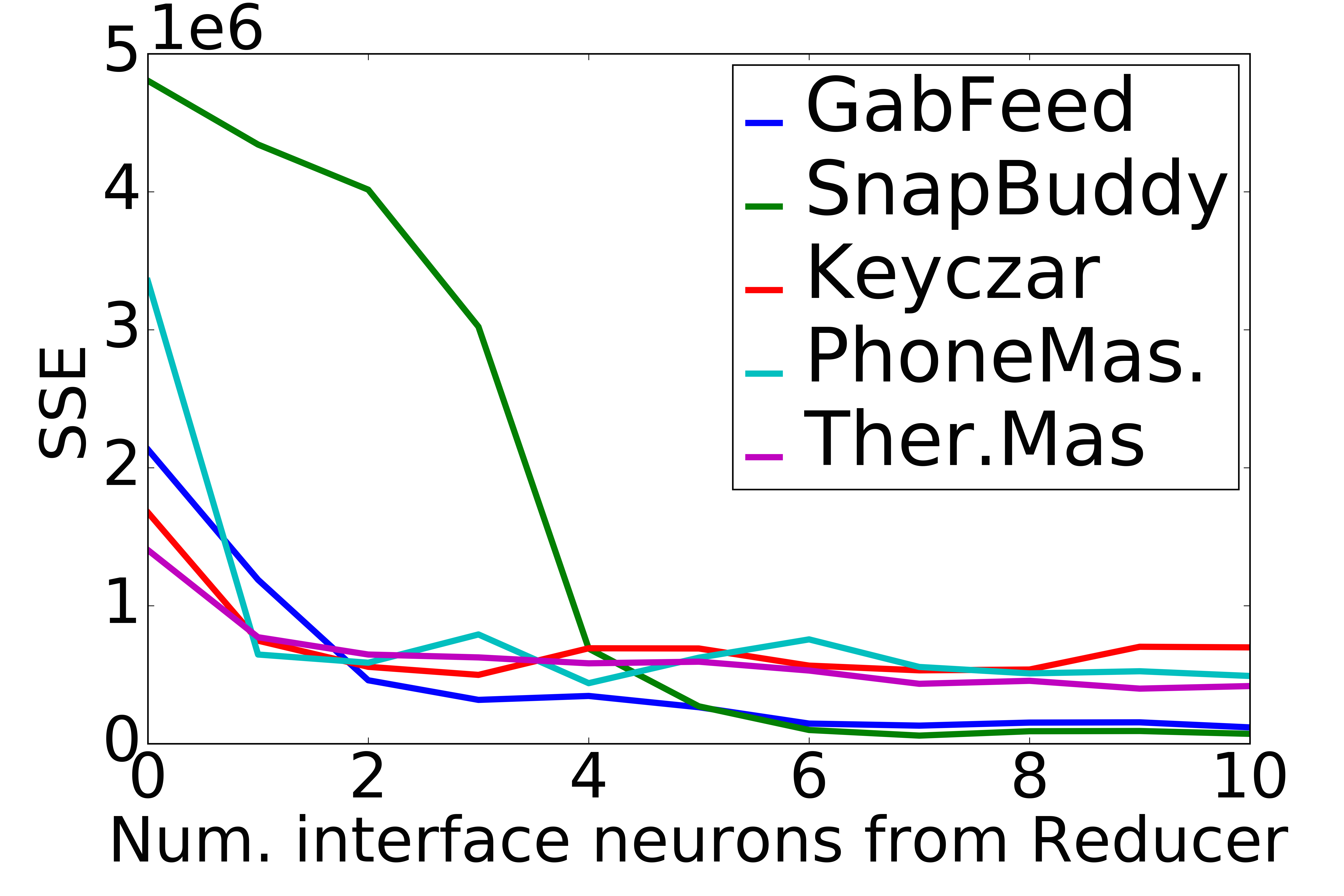
Figure 5: The SSE versus the number of interface neurons k for case-study application.

6.3 PhoneMaster

Phonemaster [6] is a record keeping service for tracking phone calls and bills. The identity of a user who submits a request is secret, while the generated traffic from the interaction is public.

Inputs. There are at most 150 users. For each user, we send a random command from the set of possible commands.

Neural Network Learning. We use a neural network with 215 neurons. We find out that the optimal number of neurons in the interface layer is 10. We learn the time model of phoneMaster in less than 10 minutes with $R^{2}=0.993$.

Security Analysis. We analyze the reducer function of NN and find out that 60 classes of observations are feasible. We assume that there can be at most 3 users in each class. The initial Shannon entropy is 7.49 bits. The remaining Shannon entropy after observing the execution times is 1.58. The amount of information leakage is 5.91 bits. This shows that almost everything about the identity of users is leaking. The computation time of analysis is about 169 minutes.

6.4 Thermomaster

Thermomaster [6] is a temperature control and prediction system. The program takes the goal temperature (secret inputs) and the current temperature (public inputs) to simulate the controller for matching with the goal temperature.

Inputs. The goal temperature is between -10,000 and +10,000 and the current temperature is between -250 and +250. We generate 10,000 inputs uniformly from the space of goal and current temperatures.

Neural Network Learning. We use a NN model with 709 neurons. The optimal number of neurons for the interface layer is 9. We learn the timing models of thermomaster in 70 minutes with $R^{2}=0.80$.

Security Analysis. We analyze the reducer function of NN and find out that only 9 classes of observations are feasible. The initial Shannon entropy is 11.0 bits. The remaining Shannon entropy after observations is 4.0. Therefore, 7.0 bits of information about the goal temperature are leaking through timing side channels. The computation time of analysis is less than 86 minutes.

6.5 Password Matching (Keyczar)

We consider a vulnerability in a password matching algorithm similar to the side-channel vulnerability in Keyczar library [34]. This vulnerability allows one to recover the secret password through sequences of oracles where the attacker learns one letter of the secret password in each step.

Inputs. The secret input is target password stored in a server, and the public input is a guess oracle. We use libFuzzer [47] to generate 21,123 guesses for randomly selected passwords. We assume a password is at most 6 (lower-case) letters.

Neural Network Learning. We use a neural network with 253 neurons. The optimal number of neurons for the interface layer is 3. We learn the time model of the password matching algorithm in 202.3 seconds with $R^{2}{=}0.976$.

Security Analysis. There can be at most 8 classes of observations. Our analysis shows only 4 classes of observations are feasible. The initial Shannon entropy is 14 bits. The 4 classes (obtained from timing observation) have the following number of elements: $\{48,6760,4309,5269\}$. So, the remaining entropy (after observing the classes through the time model) is 12.4 bits. It takes about 16 seconds to analyze the secret parts of NN and quantify the information leaks.

7 Related Work

Modeling Program Execution Times. Various techniques have been applied to model and predict computational complexity of software systems [23, 50, 7]. Both [23] and [50] consider cost measures such as execution time and predict the cost as a function of input features such as the number of bytes in an input file. The works [23, 50] are restricted to certain classes of functions such as linear functions, while the neural network techniques can model arbitrary functions. Additionally, both techniques require feature engineering: the user needs to specify some features such as size or work-load features. However, neural network models do not require this and can automatically discover important features.

Neural Networks for Security Analysis. Neural network models have been used for software security analysis. For example, the approach in [46] uses the deep neural network for anomaly detection in software defined networking (SDN). The framework [36] uses a deep neural network model for detecting vulnerabilities such as buffer and resource management errors. We use neural network models to detect and quantify information leaks through timing side channels.

Dynamic Analysis for Side-Channel Detections. Dynamic analysis has been used for side-channel detections  [38, 41, 42]. Diffuzz [41] is a fuzzing techniques for finding side channels. The approach extends AFL [1] and KELINCI [28] fuzzers to detect side channels. The goal of Diffuzz is to maximize the following objective: ${\delta=|c(p,s_{1})-c(p,s_{2})|}$, that is, to find two distinct secret values $s_{1},s_{2}$ and a public value $p$ that give the maximum cost ($c$) difference. The work [41] uses the noninterference notion of side channel leaks. Therefore, they do not quantify the amounts of information leaks. The cost function in [41] is the number of byte-code executed, whereas we consider the actual execution time in a fixed environment. Note that our approach can be used with the abstract cost model such as the byte-code executed in a straight-forward fashion. Diffuzz [41] can be combined with our technique to generate inputs and quantify leaks.

Static Analysis for Side-Channel Detections. Noninterference was first introduced by Goguen and Meseguer [22] and has been widely used to enforce confidentiality properties in various systems [43, 48, 4]. Various works [13, 5] use static analysis for side-channel detections based on noninterference notion. The work [13] defines $\varepsilon$ bounded noninterference that requires the resource usage behavior of the program executed from the same public inputs differ at most $\varepsilon$. Chen et al. [13] use Hoare Logic [11] equipped with taint analysis [37] to detect side channels. These static techniques including [13] rely on the taint analysis that is computationally difficult for real-world Java applications. The work [33] reported that 78% of 461 open-source Java projects use dynamic features such as reflections that are problematic for static analysis. In contrast, we use dynamic analysis that handles the reflections and scales well for the real-world applications. In addition, Chen et al. [13] answer either ‘yes’ or ‘no’ to the existence of side channels, which is restricted for many real-world applications that may need to disclose a small amounts of information about the secret. However, our approach quantifies the leaks using entropy measures.

Quantification of Information Leaks. Quantitative information flow [10, 44, 31] has been used for measuring the strength of side channels. The work [10] presents an approach based on finding the equivalence relation over secret inputs. The authors cast the problem of finding the equivalence relation as a reachability problem and use model counting to quantify information leaks. Their approach works only for a small program, limited to a few lines of code, while our approach can work for large applications. In addition, they consider the leaks through direct observations such as program outputs or public input values. In contrast, we consider the leaks through timing side channels, which are non-functional aspects of programs. Sidebuster [56] combines static and dynamic analyses for detection and quantification of information leaks. Sidebuster [56] also relies on taint analysis to identify the source of vulnerability. Once the source identified, Sidebuster uses dynamic analysis and measures the amounts of information leaks. The information leaks in Sidebuster [56] is because of generated network packets, while our information leaks are through timing side channels.

Hardening Against Side Channels. Hardening against side channels can be broadly divided to mitigation and elimination approaches. The mitigation approaches [32, 9, 52] aim to minimize the amounts of information leaks, while considering the performance of systems. The goal of elimination approaches [3, 55, 19] is to completely transform out information leaks without considering the performance burdens. Our techniques can be combined with the hardening methods to mitigate or eliminate information leaks.

Other Types of Side Channels. Sensitive information can be leaked through other side channels such as power consumptions [20, 53], network traffics [14], and cache behaviors [24, 45, 17, 54]. We believe our approach could be useful for these types of side channels, however, we left further analysis for future work.

8 Conclusion and Discussion

We presented a data-driven dynamic analysis for detection and quantifying information leaks due to execution times of programs. The analysis performed over a specialized NN architecture in two steps: first, we utilized neural network objects to learn timing models of programs and second, we analyzed the parts of NNs related to secret inputs to detect and quantify information leaks. Our experiences showed that NNs learn timing models of real-world applications precisely. In addition, they enabled us to quantify information leaks, thanks to the simplicity of NN models in comparison to program models.

Throughout this work, we assume that the analyzer would be able to construct interesting inputs either with fuzzing tools, previously reported bugs, or domain knowledges. Nevertheless, we demonstrate practical solutions to generate inputs in each example with emphasis on the recent development in fuzzing for side-channel analysis [41].

Furthermore, our dynamic analysis approach can not prove the absent of side channels. Our NN model learns and generalizes the timing models for the observed program behaviors and is limited to observed paths in the program. We emphasize that the proof is also difficult for static analysis. Although static analysis can prove the absent of bugs or vulnerabilities in principle, the presence of dynamic features such as reflections in Java applications is problematic and can cause false negative in static analysis (see Limitations Section in [13]).

For future work, there are few interesting directions. One idea is to develop a SAT-based algorithm, similar to DPLL, on top of MILP algorithms to calculate the number of solutions more efficiently. Another idea is to define threat models based on the attackers capabilities to utilize neural networks for guessing secrets.

Acknowledgements.

The first author thanks Shiva Darian for proofreading and providing useful suggestions. This research was supported by DARPA under agreement FA8750-15-2-0096.

References

- [1] American fuzzy lop (2016), http://lcamtuf.coredump.cx/afl/
- [2] Abadi, M., Barham, P., Chen, J., Chen, Z., Davis, A., Dean, J., Devin, M., Ghemawat, S., Irving, G., Isard, M., et al.: Tensorflow: A system for large-scale machine learning. In: OSDI’16. pp. 265–283 (2016)
- [3] Agat, J.: Transforming out timing leaks. In: Proceedings of the 27th ACM SIGPLAN-SIGACT symposium on Principles of programming languages. pp. 40–53. ACM (2000)
- [4] Almeida, J.B., Barbosa, M., Barthe, G., Dupressoir, F., Emmi, M.: Verifying constant-time implementations. In: USENIX Security Symposium. pp. 53–70 (2016)
- [5] Antonopoulos, T., Gazzillo, P., Hicks, M., Koskinen, E., Terauchi, T., Wei, S.: Decomposition instead of self-composition for proving the absence of timing channels. In: ACM SIGPLAN Notices. vol. 52, pp. 362–375. ACM (2017)
- [6] Apogee-Research: Space/time analysis for cybersecurity (stac) repository. Online: https://github.com/Apogee-Research/STAC
- [7] Arar, Ö.F., Ayan, K.: Software defect prediction using cost-sensitive neural network. Applied Soft Computing 33, 263–277 (2015)
- [8] Arora, R., Basu, A., Mianjy, P., Mukherjee, A.: Understanding Deep Neural Networks with Rectified Linear Units. arXiv e-prints (2016)
- [9] Askarov, A., Zhang, D., Myers, A.C.: Predictive black-box mitigation of timing channels. In: Proceedings of the 17th ACM conference on Computer and communications security. pp. 297–307. ACM (2010)
- [10] Backes, M., Köpf, B., Rybalchenko, A.: Automatic discovery and quantification of information leaks. In: S&P’09 (2009)
- [11] Barthe, G., D’Argenio, P.R., Rezk, T.: Secure information flow by self-composition. In: Computer Security Foundations Workshop, 2004. Proceedings. 17th IEEE. pp. 100–114. IEEE (2004)
- [12] Brumley, D., Boneh, D.: Remote timing attacks are practical. Computer Networks 48(5), 701–716 (2005)
- [13] Chen, J., Feng, Y., Dillig, I.: Precise detection of side-channel vulnerabilities using quantitative cartesian hoare logic. In: CCS (2017)
- [14] Chen, S., Wang, R., Wang, X., Zhang, K.: Side-channel leaks in web applications: A reality today, a challenge tomorrow. In: S&P’10 (2010)
- [15] Courbariaux, M., Hubara, I., Soudry, D., El-Yaniv, R., Bengio, Y.: Binarized neural networks: Training deep neural networks with weights and activations constrained to+ 1 or-1. arXiv preprint arXiv:1602.02830 (2016)
- [16] Cybenko, G.: Approximation by superpositions of a sigmoidal function. Mathematics of Control, Signals, and Systems 2, 303–314 (12 1989)
- [17] Doychev, G., Köpf, B., Mauborgne, L., Reineke, J.: Cacheaudit: A tool for the static analysis of cache side channels. ACM Transactions on Information and System Security (TISSEC) 18(1), 4 (2015)
- [18] Dutta, S., Jha, S., Sankaranarayanan, S., Tiwari, A.: Output range analysis for deep feedforward neural networks. In: NASA Formal Methods Symposium. pp. 121–138. Springer (2018)
- [19] Eldib, H., Wang, C.: Synthesis of masking countermeasures against side channel attacks. In: International Conference on Computer Aided Verification. pp. 114–130. Springer (2014)
- [20] Eldib, H., Wang, C., Schaumont, P.: Formal verification of software countermeasures against side-channel attacks. ACM Transactions on Software Engineering and Methodology (TOSEM) 24(2), 11 (2014)
- [21] Fischetti, M., Jo, J.: Deep neural networks and mixed integer linear optimization. Constraints 23(3), 296–309 (2018)
- [22] Goguen, J.A., Meseguer, J.: Security policies and security models. In: Security and Privacy, 1982 IEEE Symposium on. pp. 11–11. IEEE (1982)
- [23] Goldsmith, S.F., Aiken, A.S., Wilkerson, D.S.: Measuring empirical computational complexity. In: FSE’07. pp. 395–404. ACM (2007)
- [24] Guo, S., Wu, M., Wang, C.: Adversarial symbolic execution for detecting concurrency-related cache timing leaks. In: Proceedings of the 2018 26th ACM Joint Meeting on European Software Engineering Conference and Symposium on the Foundations of Software Engineering. pp. 377–388. ACM (2018)
- [25] Gurobi Optimization, L.: Gurobi optimizer reference manual (2018), http://www.gurobi.com
- [26] Hornik, K., Stinchcombe, M.B., White, H.: Multilayer feedforward networks are universal approximators. Neural Networks 2, 359–366 (1989)
- [27] Hund, R., Willems, C., Holz, T.: Practical timing side channel attacks against kernel space aslr. In: 2013 IEEE Symposium on Security and Privacy. pp. 191–205. IEEE (2013)
- [28] Kersten, R., Luckow, K., Păsăreanu, C.S.: Poster: Afl-based fuzzing for java with kelinci. In: Proceedings of the 2017 ACM SIGSAC Conference on Computer and Communications Security. pp. 2511–2513. ACM (2017)
- [29] Kingma, D.P., Ba, J.: Adam: A method for stochastic optimization. arXiv preprint arXiv:1412.6980 (2014)
- [30] Kocher, P.C.: Timing attacks on implementations of diffie-hellman, rsa, dss, and other systems. In: Annual International Cryptology Conference. pp. 104–113. Springer (1996)
- [31] Köpf, B., Basin, D.: An information-theoretic model for adaptive side-channel attacks. In: CCS’07. pp. 286–296 (2007)
- [32] Köpf, B., Dürmuth, M.: A provably secure and efficient countermeasure against timing attacks. In: CSF’09 (2009)
- [33] Landman, D., Serebrenik, A., Vinju, J.J.: Challenges for static analysis of java reflection-literature review and empirical study. In: 2017 IEEE/ACM 39th International Conference on Software Engineering (ICSE). pp. 507–518. IEEE (2017)
- [34] Lawson, N.: Timing attack in google keyczar library. Online post at: https://rdist.root.org/2009/05/28/timing-attack-in-google-keyczar-library/ (2009)
- [35] LeCun, Y., Bengio, Y., Hinton, G.: Deep learning. nature 521(7553), 436 (2015)
- [36] Li, Z., Zou, D., Xu, S., Ou, X., Jin, H., Wang, S., Deng, Z., Zhong, Y.: Vuldeepecker: A deep learning-based system for vulnerability detection. arXiv:1801.01681 (2018)
- [37] Livshits, V.B., Lam, M.S.: Finding security vulnerabilities in java applications with static analysis. In: USENIX Security Symposium. vol. 14, pp. 18–18 (2005)
- [38] Milushev, D., Beck, W., Clarke, D.: Noninterference via symbolic execution. In: Formal Techniques for Distributed Systems, pp. 152–168. Springer (2012)
- [39] Nagelkerke, N.J., et al.: A note on a general definition of the coefficient of determination. Biometrika 78(3), 691–692 (1991)
- [40] Narodytska, N., Kasiviswanathan, S., Ryzhyk, L., Sagiv, M., Walsh, T.: Verifying properties of binarized deep neural networks. In: AAAI’18 (2018)
- [41] Nilizadeh, S., Noller, Y., Pasareanu, C.S.: Diffuzz: Differential fuzzing for side-channel analysis. ICSE (2019), http://arxiv.org/abs/1811.07005
- [42] Rosner, N., Burak Kadron, I., Bang, L., Bultan, T.: Profit: Detecting and quantifying side channels in networked applications. NDSS (2019)
- [43] Sabelfeld, A., Myers, A.C.: Language-based information-flow security. IEEE Journal on selected areas in communications (2003)
- [44] Smith, G.: On the foundations of quantitative information flow. In: FoSSaCS’09 (2009)
- [45] Sung, C., Paulsen, B., Wang, C.: Canal: A cache timing analysis framework via llvm transformation. pp. 904–907. ASE 2018
- [46] Tang, T.A., Mhamdi, L., McLernon, D., Zaidi, S.A.R., Ghogho, M.: Deep learning approach for network intrusion detection in software defined networking. In: WINCOM’16 (2016)
- [47] libFuzzer team, G.: Libfuzzer: Coverage-based fuzz testing. Online: http://llvm.org/docs/LibFuzzer.html (2016)
- [48] Terauchi, T., Aiken, A.: Secure information flow as a safety problem. In: International Static Analysis Symposium. pp. 352–367. Springer (2005)
- [49] Tizpaz-Niari, S., Černý, P., Chang, B.Y.E., Sankaranarayanan, S., Trivedi, A.: Discriminating traces with time. In: TACAS’17. pp. 21–37. Springer (2017)
- [50] Tizpaz-Niari, S., Černý, P., Chang, B.E., Trivedi, A.: Differential performance debugging with discriminant regression trees. In: AAAI’18. pp. 2468–2475 (2018)
- [51] Tizpaz-Niari, S., Černý, P., Trivedi, A.: Data-driven debugging for functional side channels. arXiv:1808.10502 (2018)
- [52] Tizpaz-Niari, S., Černý, P., Trivedi, A.: Quantitative mitigation of timing side channels. In: Computer Aided Verification (CAV). pp. 140–160 (2019)
- [53] Wang, J., Sung, C., Wang, C.: Mitigating power side channels during compilation. arXiv preprint arXiv:1902.09099 (2019)
- [54] Wang, S., Wang, P., Liu, X., Zhang, D., Wu, D.: Cached: Identifying cache-based timing channels in production software. In: 26th USENIX Security Symposium. pp. 235–252 (2017)
- [55] Wu, M., Guo, S., Schaumont, P., Wang, C.: Eliminating timing side-channel leaks using program repair. In: Proceedings of the 27th ACM SIGSOFT International Symposium on Software Testing and Analysis. pp. 15–26. ACM (2018)
- [56] Zhang, K., Li, Z., Wang, R., Wang, X., Chen, S.: Sidebuster: automated detection and quantification of side-channel leaks in web application development. In: Proceedings of the 17th ACM conference on Computer and communications security. pp. 595–606. ACM (2010)