Mix and Match: An Optimistic Tree-Search Approach for Learning Models from Mixture Distributions

Abstract

We consider a covariate shift problem where one has access to several different training datasets for the same learning problem and a small validation set which possibly differs from all the individual training distributions. This covariate shift is caused, in part, due to unobserved features in the datasets. The objective, then, is to find the best mixture distribution over the training datasets (with only observed features) such that training a learning algorithm using this mixture has the best validation performance. Our proposed algorithm, Mix&Match, combines stochastic gradient descent (SGD) with optimistic tree search and model re-use (evolving partially trained models with samples from different mixture distributions) over the space of mixtures, for this task. We prove simple regret guarantees for our algorithm with respect to recovering the optimal mixture, given a total budget of SGD evaluations. Finally, we validate our algorithm on two real-world datasets.

1 Introduction

The problem of covariate shift – where the distribution on the covariates is different across the training and validation datasets – has long been appreciated as an issue of central importance for real-world problems (e.g., Shimodaira, (2000); Gretton et al., (2009) and references therein). Covariate shift is often ascribed to a changing population, bias in selection, or imperfect, noisy or missing measurements. Across these settings, a number of approaches to mitigate covariate shift attempt to re-weight the samples of the training set in order to match the target set distribution Shimodaira, (2000); Zadrozny, (2004); Huang et al., (2007); Gretton et al., (2009). For example, Huang et al., (2007); Gretton et al., (2009) use unlabeled data to compute a good kernel reweighting.

We consider a setting where covariate shift is due to unobserved variables in different populations (datasets). A motivating example is the setting of predictive health care in different regions of the world. Here, the unobserved variables may represent, for example, prevalence and expression of different conditions, genes, etc. in the makeup of the population. Another key example, and one for which we have real-world data (see Section 7), is predicting what insurance plan a customer will purchase, in a given state. The unobserved variables in this setting might include employment information (security at work), risk-level of driving, or state-specific factors such as weather or other driving-related features. Motivated by such applications, we consider the setting where the joint distribution (of observed, unobserved variables and labels) may differ across various populations, but the conditional distribution of the label (conditioned on both observed and unobserved variables) remains invariant. The goal, then, is to determine a mixture distribution over the input datasets (training populations) in order to optimize performance on the validation set.

The contributions in this paper are as follows:

(i) Search based methods for covariate shift: With latent/unobserved features, we show in Section 4 that traditional methods such as moment matching cannot learn the best mixture distribution (over input datasets) that optimizes performance with respect to a validation set. Instead, we show that searching over input mixture distributions using validation loss results in the recovery of the true model (with respect to the validation, Proposition 1). This motivates our tree search based approach.

(ii) Mix&Match – Optimistic tree search over models: We propose Mix&Match – an algorithm that is built on SGD and a variant of optimistic tree-search (closely related to Monte Carlo Tree Search). Given a budget (denoted as $\Lambda$) on the total number of online SGD iterations, Mix&Match adaptively allocates this budget to different population reweightings (mixture distributions over input datasets) through an iterative tree-search procedure (Section 5). Importantly, Mix&Match expends a majority of the SGD iteration budget on reweightings that are "close" to the optimal reweighting mixture by using two important ideas:
(a) Parsimony in expending iterations: For a reweighting distribution that we have low confidence of being “good,” Mix&Match expends only a small number of SGD iterations to train the model; doing so, however, results in biased and noisy evaluation of this model, due to early stopping in training.
(b) Re-use of models: Rather than train a model from scratch, Mix&Match reuses and updates a partially trained model from past reweightings that are “close” to the currently chosen reweighting (effectively re-using SGD iterations from the past).

(iii) SGD concentrations without global gradient bounds: The analysis of Mix&Match requires a new concentration bound on the error of the final iterate of SGD. Instead of assuming a uniform bound on the norm of the stochastic gradient over the domain, as is typical in the stochastic optimization literature, we directly exploit properties of the averaged loss (strong convexity) and individual loss (smoothness) combined with a bound on the norm of the stochastic gradient at a single point to bound the norm of the stochastic gradient at each iterate. Using a single parameter ($\Lambda$, the budget allocated to Mix&Match), we are able to balance the worst-case growth of the norm of the stochastic gradient with the probability of failure of the SGD concentration. This new result (Theorem 2) provides tighter high-probability guarantees on the error of the final SGD iterate in settings where the diameter of the domain is large and/or cannot be controlled.

2 Related Work

Transfer learning has assumed an increasingly important role, especially in settings where we are either computationally limited or data-limited but can leverage significant computational and data resources on domains that differ slightly from the target domain Raina et al., (2007); Pan and Yang, (2009); Dai et al., (2009). This has become an important paradigm in neural networks and other areas Bengio, (2011); Yosinski et al., (2014); Oquab et al., (2014); Kornblith et al., (2018). A related problem is that of covariate shift Shimodaira, (2000); Zadrozny, (2004); Gretton et al., (2009), where the target population distribution may differ from that of the training distribution. Some recent works have considered addressing this problem by reweighting samples from the training dataset so that the distribution better matches the test set, for example by using unlabelled data Huang et al., (2007); Gretton et al., (2009) or variants of importance sampling Sugiyama et al., (2007, 2008). The authors in Mohri et al., (2019) study a related problem of learning from different datasets, but provide minimax bounds in terms of an agnostically chosen test distribution.

Our work is related to, but differs from all the above. As we explain in Section 3, we share the goal of transfer learning: we have access to enough data for training from a family of distributions that are different than the validation distribution (from which we have only enough data to validate). However, to address the effects of latent features, we adopt an optimistic tree search approach – something that, as far as we know, has not been undertaken.

A key component of our tree-search based approach to the covariate shift problem is the computational budget. We use a single SGD iteration as the currency denomination of our budget, which requires us to minimize the number of SGD steps in total that our algorithm computes, and thus to understand the final-iterate optimization error of SGD in high probability. There are many works deriving error bounds on the final SGD iterate in expectation (e.g. Bubeck, (2015); Bottou et al., (2018); Nguyen et al., (2018)) and in high probability (e.g. Rakhlin et al., (2012); Harvey et al., (2018) and references therein). However, to our knowledge, optimization error bounds on the final iterate of SGD when the stochastic gradient is assumed bounded only at the optimal solution exist only in expectation Nguyen et al., (2018). We prove a similar result in high probability.

Optimistic tree search makes up the final important ingredient in our algorithm. These ideas have been used in a number of settings Bubeck et al., (2011); Grill et al., (2015). Most relevant to us is a recent extension of these ideas to a setting with biased search Sen et al., (2018, 2019).

3 Problem Setting and Model

3.1 Data model

Each dataset $\mathcal{D}$ consists of samples of the form $z=(\boldsymbol{x},y)\in\mathbb{R}^{d}\times\mathbb{R}$, where $\boldsymbol{x}$ corresponds to the observed feature vector, and $y$ is the corresponding label. Traditionally, we would regard dataset $\mathcal{D}$ as governed by a distribution $p(\boldsymbol{x},y)$. However, we consider the setting where each sample $z$ is a projection from some higher dimensional vector $\hat{z}=(\boldsymbol{x},\boldsymbol{u},y)$, where $\boldsymbol{u}\in\mathbb{R}^{\hat{d}}$ is the unobserved feature vector. The corresponding distribution function describing the dataset is thus $p(\boldsymbol{x},\boldsymbol{u},y)$. This viewpoint allows us to model, for example, predictive healthcare applications where the unobserved features $\boldsymbol{u}$ could represent uncollected, region specific information that is potentially useful in the prediction task (e.g., dietary preferences, workday length, etc.).

We assume access to $K$ training datasets $\{\mathcal{D}_{i}\}_{i=1}^{K}$ (e.g., data for a predictive healthcare task collected in $K$ different countries) with corresponding p.d.f.’s $\{p_{i}(\boldsymbol{x},\boldsymbol{u},y)\}_{i=1}^{K}$ through a sample oracle to be described shortly. Taking $\triangle:=\{\boldsymbol{\alpha}\in\mathbb{R}^{K}:\boldsymbol{\alpha}\succeq\boldsymbol{0},\|\boldsymbol{\alpha}\|_{1}=1\}$ as the $(K-1)$-dimensional mixture simplex, for any $\boldsymbol{\alpha}\in\triangle$, we denote the mixture distribution over the training datasets as $p^{(\boldsymbol{\alpha})}(\boldsymbol{x},\boldsymbol{u},y):=\sum_{i=1}^{K}\boldsymbol{\alpha}_{i}p_{i}(\boldsymbol{x},\boldsymbol{u},y)$. Samples from these datasets may be obtained through a sample oracle which, given a mixture $\boldsymbol{\alpha}$, returns an independent sample from the corresponding mixture distribution. In the healthcare example, sampling from $p^{(\boldsymbol{\alpha})}$ would mean first sampling an index $i$ from the multinomial distribution represented by $\boldsymbol{\alpha}$ and then drawing a new medical record from the database of the $i$th country. Additionally, we have access to a small (see Remark 1) validation dataset $\mathcal{D}_{te}$ with corresponding distribution $p^{(te)}(\boldsymbol{x},\boldsymbol{u},y)$, for example, from a new country where only limited data has been collected. We are interested in training a predictive model for the validation distribution, but we do not have oracle sampling access to this distribution – if we did, we could simply train a model through SGD directly on this dataset. Instead, we only assume oracle access to evaluating the validation loss of a constrained set of models (we define our loss model and the constrained set shortly). We make the following assumptions on the validation distribution:

Assumption 1.

We assume that the marginal distribution of observed and unobserved features for the validation distribution lies in the convex hull of the corresponding training distributions – that is, there exists some $\boldsymbol{\alpha}^{*}\in\triangle$ such that $p^{(te)}(\boldsymbol{x},\boldsymbol{u})=p^{(\boldsymbol{\alpha}^{*})}(\boldsymbol{x},\boldsymbol{u})$.

Additionally, we make the following assumption on the conditional distribution of the validation labels, which we refer to as conditional shift invariance:

Assumption 2 (Conditional Shift Invariance).

We assume that the distribution of labels conditioned on both observed and unobserved features is fixed for all training and validation distributions. That is, for each $i\in[K]$

$$p_{i}(y|\boldsymbol{x},\boldsymbol{u})=p(y|\boldsymbol{x},\boldsymbol{u})=p^{(te)}(y|\boldsymbol{x},\boldsymbol{u})$$

for some fixed distribution $p$.

We note that Assumption 2 generalizes the covariate shift assumption of Heckman, (1977); Shimodaira, (2000) ($p(y|x)$ is fixed) to account for latent variables.

3.2 Loss function model

We denote the loss for a particular sample $z$ and model $\boldsymbol{w}\in\mathcal{W}:=\mathbb{R}^{m}$ as $f(\boldsymbol{w};z).$ For any mixture distribution $\boldsymbol{\alpha}\in\triangle$, we denote $F^{(\boldsymbol{\alpha})}(\boldsymbol{w}):=\mathbb{E}_{z\sim p^{(\boldsymbol{\alpha})}}[f(\boldsymbol{w};z)]$ as the averaged loss function over distribution $p^{(\boldsymbol{\alpha})}$. Note that when $\boldsymbol{\alpha}$ is clear from context, we write $F(\boldsymbol{w})$. Similarly, we denote $F^{(te)}(\boldsymbol{w}):=\mathbb{E}_{z\sim p^{(te)}}[f(\boldsymbol{w};z)]$ as the averaged validation loss. We place the following assumptions on our loss function, similar to Nguyen et al., (2018) (refer to Appendix B for these standard definitions):

Assumption 3.

For each loss function $f(\cdot;z)$ corresponding to a sample $z\in\mathcal{Z}$, we assume that $f(\cdot;z)$ is: (i) $\beta$-smooth and (ii) convex.

Additionally, we assume that, for each $\boldsymbol{\alpha}\in\triangle$, the averaged loss function $F^{(\boldsymbol{\alpha})}(\cdot)$ is: (i) $\mu$-strongly convex and (ii) $L$-Lipschitz.

Notice that Assumption 3 requires only the averaged loss function $F^{(\boldsymbol{\alpha})}(\cdot)$ – not each individual loss function $f(\cdot;z)$ – to be strongly convex. We additionally assume the following bound on the gradient of $f$ at $\boldsymbol{w}^{*}$ along every sample path:

Assumption 4 (A weaker gradient norm bound).

For all $\boldsymbol{\alpha}\in\triangle$, there exists constants $\mathcal{G}_{*}(\boldsymbol{\alpha})\in\mathbb{R}_{+}$ such that $\|\nabla f(\boldsymbol{w}^{*}(\boldsymbol{\alpha});z)\|_{2}^{2}\leq\mathcal{G}_{*}{(\boldsymbol{\alpha})}.$ When $\boldsymbol{\alpha}$ is clear from context, we write $\mathcal{G}_{*}.$

We note that Assumption 4 is weaker than the typical universal bound on the norm of the stochastic gradient assumed in, for example, Rakhlin et al., (2012); Harvey et al., (2018), and is taken from Nguyen et al., (2018).

4 Problem Formulation

Given $K$ training datasets $\{\mathcal{D}_{i}\}_{i=1}^{K}$ (e.g., healthcare data from $K$ countries) and a small (see Remark 1), labeled validation dataset $\mathcal{D}_{te}$ (e.g., preliminary data collected in a new country), we wish to find a model $\hat{\boldsymbol{w}}$ such that the loss averaged over the validation distribution, $p^{(te)}$, is as small as possible, using a computational budget to be described shortly. Under the notation introduced in Section 3, we wish to approximately solve the optimization problem:

$$\min_{\boldsymbol{w}\in\mathcal{W}}F^{(te)}(\boldsymbol{w}),$$ (1)

subject to a computational budget of $\Lambda$ SGD iterations. A computational budget is often used in online optimization as a model for constraints on the number of i.i.d. samples available to the algorithm (see for example the introduction to Chapter 6 in Bubeck, (2015)).

Note that one could run SGD directly on the validation dataset, $\mathcal{D}_{te}$, in order to minimize the expected loss on this population, as long as the number of SGD steps is linear in the size of $\mathcal{D}_{te}$ Hardt et al., (2015). When the number of validation samples is small relative to the computational budget $\Lambda$, such as in the predictive healthcare example where little data from the new target country is available, the resulting error guarantees of such a procedure will be correspondingly weak. Thus, we hope to leverage both training data and validation data in order to solve (1).

Though we cannot train a model using $\mathcal{D}_{te}$, we will assume $\mathcal{D}_{te}$ is sufficiently large to obtain an accurate estimate of the validation loss. We model evaluations of validation loss through oracle access to $F^{(te)}(\cdot)$, which may be queried only on models trained by running at least one SGD iteration on some mixture distribution over the training datasets.

Remark 1 (Small validation dataset regime).

Under no assumptions on the usage of the (size $n$) validation set, only $k~{}=~{}O(n^{2})$ queries can be made while maintaining nontrivial generalization guarantees Bassily et al., (2016); Mania et al., (2019). When tracking only the best model, as in Blum and Hardt, (2015); Hardt, (2017), $k$ can be roughly exponential in the size of the validation set. While our setting is more similar to this latter setting, a precise characterization of the sample complexity, and thus of the precise bounds on the size of the validation set, is important. Here we focus on the computational aspects, and leave the formalization of generalization guarantees in our setting to future work.

Let $\boldsymbol{w}^{*}(\boldsymbol{\alpha}):=\operatorname*{arg\,min}_{\boldsymbol{w}\in\mathcal{W}}F^{(\boldsymbol{\alpha})}(\boldsymbol{w})$ be the optimal model for training mixture distribution $p^{(\boldsymbol{\alpha})}$. Similarly, let us denote $\hat{\boldsymbol{w}}(\boldsymbol{\alpha})$ as the model obtained after running $1\leq T\leq\Lambda$ steps of online SGD on $p^{(\boldsymbol{\alpha})}$. Then we can minimize validation loss $F^{(te)}(\cdot)$ by (i) iteratively selecting mixtures $\boldsymbol{\alpha}\in\triangle$, (ii) using a portion of the SGD budget to solve for $\hat{\boldsymbol{w}}(\boldsymbol{\alpha})$, and (iii) evaluating the quality of the selected mixture by obtaining the validation loss $F^{(te)}(\hat{\boldsymbol{w}}(\boldsymbol{\alpha}))$ (through oracle access, as discussed earlier). That is, using $\Lambda$ total SGD iterations, we can find a mixture distribution $\boldsymbol{\alpha}(\Lambda)$ and model $\hat{\boldsymbol{w}}(\boldsymbol{\alpha}(\Lambda))$ so that $F^{(te)}(\hat{\boldsymbol{w}}(\Lambda))$ is as close as possible to

$$\min_{\boldsymbol{\alpha}\in\triangle}G(\boldsymbol{\alpha})=\min_{\boldsymbol{\alpha}\in\triangle}F^{(te)}(\boldsymbol{w}^{*}(\boldsymbol{\alpha})),$$ (2)

where $G(\boldsymbol{\alpha}):=F^{(te)}(\boldsymbol{w}^{*}(\boldsymbol{\alpha}))$ is the test loss evaluated at the optimal model for $p^{(\boldsymbol{\alpha})}$.

Under our Assumptions 1 and 2, we have the following connection between training and validation loss, which establishes that solving (1) and (2) are equivalent:

Proposition 1.

By Assumptions 1 and 2, the validation loss can be written in terms of mixtures of training loss:

$$F^{(te)}(\boldsymbol{w})=F^{(\boldsymbol{\alpha}^{*})}(\boldsymbol{w})$$ (3)

for each $\boldsymbol{w}\in\mathcal{W}$, where $\boldsymbol{\alpha}^{*}$ is the mixture specified by Assumption 1. As a consequence, finding $\boldsymbol{w}^{*}$ which solves (1) is equivalent to finding the mixture $\boldsymbol{\alpha}^{*}$ and corresponding model $\boldsymbol{w}^{*}(\boldsymbol{\alpha}^{*})$ which solves (2), since $F^{(te)}(\boldsymbol{w}^{*})=F^{(\boldsymbol{\alpha}^{*})}(\boldsymbol{w}^{*})=F^{(\boldsymbol{\alpha}^{*})}(\boldsymbol{w}^{*}(\boldsymbol{\alpha}^{*}))$.

Proposition 1 follows immediately by noting that, from Assumptions 1 and 2, $p^{(te)}(\boldsymbol{x},\boldsymbol{u},y)=p^{(\boldsymbol{\alpha}^{*})}(\boldsymbol{x},\boldsymbol{u},y)$, and thus $p^{(te)}(\boldsymbol{x},y)=p^{(\boldsymbol{\alpha}^{*})}(\boldsymbol{x},y)$, and using the definition of $F^{(te)}$.

We take as our objective to minimize simple regret with respect to the optimal model $\boldsymbol{w}^{*}(\boldsymbol{\alpha}^{*})$:

$$R(\Lambda):=G(\boldsymbol{\alpha}(\Lambda))-\min_{\boldsymbol{\alpha}\in\triangle}G(\boldsymbol{\alpha}).$$ (4)

That is, we measure the performance of our algorithm by the difference in validation loss between the best model corresponding to our final selected mixture, $\boldsymbol{w}^{*}(\boldsymbol{\alpha}(\Lambda))$ and the best model for the validation loss, $\boldsymbol{w}^{*}(\boldsymbol{\alpha}^{*})$.

Remark 2 (Difficulties with moment matching and domain invariant representations).

Note that we cannot learn $\boldsymbol{\alpha}^{*}$ simply by matching the mixture distribution over the training sets to that of the validation set (both with only the observed features and labels). This is because $p_{k}(x,u)$ decomposes as $p_{k}(x,u)=p_{k}(x)p_{k}(u|x),$ where $p_{k}(u|x)$ is unknown and potentially differs across datasets. Thus, in a setting with unobservable features, approaches that try to directly learn the mixture weights by comparing with the validation set (e.g., using an MMD distance or moment matching) learns the wrong mixture weights. Further, our scenario also admits cases where the observed $p(y|x)$ (label distribution conditioned on observed variables) can shift which is non-trivial. In fact, when observed conditional distribution of labels differ between training and validation, strong lower bounds exist on many variants of another popular method called domain invariant representation (see Corollary $4.1$ in Zhao et al., (2019)).

5 Algorithm

We now present Mix&Match (Algorithm 1), our proposed algorithm for minimizing $G(\boldsymbol{\alpha})=F^{(te)}(\boldsymbol{w}^{*}(\boldsymbol{\alpha}))$ over the mixture simplex $\triangle$ using $\Lambda$ total SGD iterations. To solve this minimization problem, our algorithm must search over the mixture simplex, and for each $\boldsymbol{\alpha}\in\triangle$ selected by the algorithm, approximately evaluate $G(\boldsymbol{\alpha})$ by obtaining an approximate minimizer $\hat{\boldsymbol{w}}(\boldsymbol{\alpha})$ of $F^{(\boldsymbol{\alpha})}(\cdot)$ and evaluating $\widehat{G}(\boldsymbol{\alpha})=F^{(\boldsymbol{\alpha})}(\hat{\boldsymbol{w}}(\boldsymbol{\alpha}))$. Two main ideas underlie our algorithm: parsimony in expending SGD iterations – using a small number of iterations for mixture distributions that we have a low confidence are “good” – and model reuse – using models trained on nearby mixtures as a starting point for training a model on a new mixture distribution. We now outline why and how the algorithm utilizes these two ideas. In Section 6, we formalize these ideas.

Warming up: model search with optimal mixture. By Proposition 1, $G(\boldsymbol{\alpha})=F^{(\boldsymbol{\alpha}^{*})}(\boldsymbol{w}^{*}(\boldsymbol{\alpha}))$ for all $\boldsymbol{\alpha}\in\triangle.$ Therefore, if we were given $\boldsymbol{\alpha}^{*}$ a priori, then we could run stochastic gradient descent to minimize the loss over this mixture distribution on the training datasets, $F^{(\boldsymbol{\alpha}^{*})}(\cdot)$, in order to find an $\varepsilon-$approximate solution to $\boldsymbol{w}^{*}(\boldsymbol{\alpha}^{*})$, the desired optimal model for the validation distribution. In our experiments (Sections 7 and Appendix G), we will refer to this algorithm as the Genie. Our algorithm, thus, will be tasked to find a mixture close to $\boldsymbol{\alpha}^{*}$.

Close mixtures imply close optimal models. Now, suppose that instead of being given $\boldsymbol{\alpha}^{*}$, we were given some other $\hat{\boldsymbol{\alpha}}\in\triangle$ which is close to $\boldsymbol{\alpha}^{*}$ in $\ell_{1}$ distance. Then, as we will prove in Corollary 1, we know that the optimal model for this alternate distribution $\boldsymbol{w}^{*}(\hat{\boldsymbol{\alpha}})$ is close to $\boldsymbol{w}^{*}(\boldsymbol{\alpha}^{*})$ in $\ell_{2}$ distance, and additionally, $G(\hat{\boldsymbol{\alpha}})$ is close to $G(\boldsymbol{\alpha}^{*})$. In fact, this property is not special to mixtures close to $\boldsymbol{\alpha}^{*}$, but holds more generally for any two mixtures that are close in $\ell_{1}$ distance. Thus, our algorithm needs only to find a mixture $\hat{\boldsymbol{\alpha}}$ sufficiently close to $\boldsymbol{\alpha}^{*}$.

Smoothness of $G(\cdot)$ and existence of “good” simplex partitioning implies applicability of optimistic tree search algorithms. This notion of smoothness of $G(\boldsymbol{\alpha})$ immediately implies that we can use the optimistic tree search framework similar to Bubeck et al., (2011); Grill et al., (2015) in order to minimize $G(\boldsymbol{\alpha})$ by performing a tree search procedure over hierarchical partitions of the mixture simplex $\triangle$ – indeed, in this literature, such smoothness conditions are directly assumed. Additionally, the existence of a hierarchical partitioning such that the diameter of each partition cell decays exponentially with tree height is also assumed. In our work, however, we prove in Corollary 1 that the smoothness condition on $G(\cdot)$ holds, and by using the simplex bisection strategy described in Kearfott, (1978), the cell diameter decay condition also holds. Thus, it is natural to design our algorithm in the tree search framework.

Tree search framework. Mix&Match proceeds by constructing a binary partitioning tree $\mathcal{T}$ over the space of mixtures $\triangle$. Each node $(h,i)\in\mathcal{T}$ is indexed by the height (i.e. distance from the root node) $h$ and the node’s index $i\in[2^{h}]$ in the layer of nodes at height $h$. The set of nodes $V_{h}=\{(h,i):i\in[2^{h}]\}$ at height $h$ are associated with a partition $\mathcal{P}_{h}=\{\mathcal{P}_{h,i}:i\in[2^{h}]\}$ of the mixture simplex $\triangle$ into $2^{h}$ disjoint partition cells whose union is $\triangle$. The root node $(0,1)$ is associated with the entire simplex $\triangle$, and two children of node $(h,i)$, $\{(h+1,2i-1),(h+1,2i)\}$ correspond to the two partition cells of the parent node’s partition. The resulting hierarchical partitioning will be denoted $\mathcal{P}=\cup_{h}\mathcal{P}_{h}$, and can be implemented using the simplex bisection strategy of Kearfott, (1978). Combined with the smoothness results on our objective function, $\mathcal{T}$ gives a natural structure to search for $\boldsymbol{\alpha}^{*}$.

Multi-fidelity evaluations of $G(\cdot)$ – associating $\mathcal{T}$ with mixtures and models. We note that, in our setting, $G(\boldsymbol{\alpha})=F^{(te)}(\boldsymbol{w}^{*}(\boldsymbol{\alpha}))$ cannot be directly evaluated, since we cannot obtain $\boldsymbol{w}^{*}(\boldsymbol{\alpha})$ explicitly, but only an approximate minimizer $\hat{\boldsymbol{w}}(\boldsymbol{\alpha})$. Thus, we take inspiration from recent works in multi-fidelity tree-search Sen et al., (2018, 2019). Specifically, using a height-dependent SGD budget function $\lambda(h)$, the algorithm takes $\lambda(h;\delta)$ SGD steps using some selected mixture $\boldsymbol{\alpha}_{h,i}\in\mathcal{P}_{h,i}$ to obtain an approximate minimizer $\hat{\boldsymbol{w}}(\boldsymbol{\alpha}_{h,i})$ and evaluates the validation loss $F^{(te)}(\hat{\boldsymbol{w}}(\boldsymbol{\alpha}_{h,i}))$ to obtain an estimate for $G(\boldsymbol{\alpha}_{h,i})$. $\lambda(\cdot)$ is designed so that estimates of $G(\cdot)$ are “crude” early during the tree-search procedure and more refined deeper in the search tree.

Warm starting with the parent model. When our algorithm, Mix&Match selects node $(h,i)$, it creates child nodes $\{(h+1,2i-1),(h+1,2i)\}$, and runs SGD on the associated mixtures $\boldsymbol{\alpha}_{h+1,2i-1}$ and $\boldsymbol{\alpha}_{h+1,2i}$, starting each SGD run with initial model $\hat{\boldsymbol{w}}(\boldsymbol{\alpha}_{h,i})$, the final iterate of the parent node’s SGD run. Since $\boldsymbol{\alpha}_{h,i}$ and $\boldsymbol{\alpha}_{h+1,j}$ ($j\in\{2i-1,2i\}$) are exponentially close as a function of $h$ (as a consequence of our simplex partitioning strategy), so too are $\boldsymbol{w}^{*}(\boldsymbol{\alpha}_{h,i})$ and $\boldsymbol{w}^{*}(\boldsymbol{\alpha}_{h+1,j})$ (since close mixtures implies close models). Thus, as long as the parent’s final iterate is exponentially close to $\boldsymbol{w}^{*}(\boldsymbol{\alpha}_{h,i})$, then the initial iterate for the SGD runs associated to the child nodes will also be exponentially close to their associated solution, $\boldsymbol{w}^{*}(\boldsymbol{\alpha}_{h+1,j})$. This implies that that a good initial condition of weights for a child node’s model is that resulting from the final iterate of the parent’s model.

Constant SGD steps suffice for exponential error improvement. In a noiseless setting (e.g., the setting of Theorem 3.12 in Bubeck, (2015)), optimization error scales linearly in the squared distance between the initial model and the optimal model, and thus, in this setting, we could simply take a constant number of gradient descent steps to obtain a model with error exponential in $h+1$. However, in SGD, optimization error depends not only on the initial distance to the optimal model, but also on the noise of the stochastic gradient. Under our $\beta$-smoothness assumption and Assumption 4, however, we can show that, until we hit the noise floor of $\mathcal{G}_{*}(\boldsymbol{\alpha})$ (the bound on the norm of the gradient only at the optimal model $\boldsymbol{w}^{*}(\boldsymbol{\alpha})$), the noise of the stochastic gradient also decays exponentially with tree height (see e.g. Lemma 3 in the Appendix for a proof). As a consequence, until we hit this noise floor, we may take a constant number of SGD steps to exponentially improve the optimization error as we descend our search tree. In fact, all of our experiments (Section 7 and Appendix G) use a height-independent budget function $\lambda$.

Growing the search tree. Mix&Match constructs the search tree in the same manner as MFDOO from Sen et al., (2018). Initially, $\mathcal{T}=\{(0,1)\}$, and until the SGD budget $\Lambda$ has been exhausted, the algorithm proceeds by selecting the node $(h,i)$ from the set of leaf nodes that has the smallest estimate (denoted $b_{h,i}$) for $G(\cdot)$ for any mixture within the leaf’s corresponding partition cell, $\mathcal{P}_{h,i}$. In this manner, we can expect to obtain similar simple regret guarantees as those obtained for MFDOO.

Algorithm 1 Mix&Match: Tree-Search over the mixtures of training datasets

0:  Real numbers $\nu_{2}>0$, $\rho_{2}\in(0,1)$ as specified in Corollary 1, hierarchical partition $\mathcal{P}$ of $\triangle$, SGD budget $\Lambda\geq 0$.

1:  Expand the root node using Algorithm 2 and form two leaf nodes $\mathcal{T}_{t}=\{(1,1),(1,2)\}$.

2:  Cost (Number of SGD steps used): $C=2\lambda(0)$

3:  while $C\leq\Lambda$ do

4:     Select the leaf $(h,j)\in\mathrm{Leaves}(\mathcal{T}_{t})$ with minimum $b_{h,j}:=F^{(te)}(\hat{\boldsymbol{w}}(\boldsymbol{\alpha}_{h,j}))-2\nu_{2}\rho_{2}^{h}$.

5:     Add to $\mathcal{T}_{t}$ the $2$ children of $(h,j)$ (as determined by $\mathcal{P})$ by querying them using Algorithm 2.

6:     $C=C+2\lambda(h+1)$.

7:  end while

8:  Let $h(\Lambda)$ be the height of $\mathcal{T}_{t}$

9:  Let $i^{*}:=\operatorname*{arg\,min}_{{i}}F^{(te)}(\hat{\boldsymbol{w}}(\boldsymbol{\alpha}_{h(\Lambda),i}))$.

10:  Return $\boldsymbol{\alpha}_{h(\Lambda),i^{*}}$ and $\hat{\boldsymbol{w}}(\boldsymbol{\alpha}_{h(\Lambda),i^{*}})$.

Algorithm 2 ExpandNode: Optimize over the current mixture and evaluate

0:  Parent node $(h,i)$ with model $\hat{\boldsymbol{w}}(\boldsymbol{\alpha}_{h,i})$, $\nu_{2}>0$, $\rho_{2}~{}\in~{}(0,1)$

1:  // Iterate over new child node indices

2:  for $(h^{\prime},i^{\prime})\in\{(h+1,2i-1),(h+1,2i)\}$ do

3:     Let $\boldsymbol{\alpha}:=\boldsymbol{\alpha}_{h^{\prime},i^{\prime}}\in\mathcal{P}_{h^{\prime},i^{\prime}}$ and $\boldsymbol{w}_{0}:=\hat{\boldsymbol{w}}(\boldsymbol{\alpha}_{h,i})$.

4:     for $t=1,...,T:=\lambda(h)$ (see Corollary 2) do

5:        $\boldsymbol{w}_{t}=\boldsymbol{w}_{t-1}-\eta_{t}\nabla f(\boldsymbol{w}_{t-1};z_{t})$ for $z_{t}\sim p^{(\boldsymbol{\alpha})}$.

6:     end for

7:     Obtain test error $F^{(te)}(\boldsymbol{w}_{T})$

8:     Set node estimate: $b_{h^{\prime},i^{\prime}}=F^{(te)}(\boldsymbol{w}_{T})-2\nu_{2}\rho_{2}^{h^{\prime}}.$

9:     Set final model: $\hat{\boldsymbol{w}}(\boldsymbol{\alpha}_{h^{\prime},i^{\prime}})=\boldsymbol{w}_{T}$.

10:  end for

6 Theoretical Results

We now present the theoretical results which formalize the intuition outlined in Section 5. All proofs can be found in the Appendix.

6.1 Close mixtures imply close solutions

Our first result shows that the optimal weights with respect to the two distributions $p^{(\boldsymbol{\alpha}_{1})}$ and $p^{(\boldsymbol{\alpha}_{2})}$ are close, if the mixture weights $\boldsymbol{\alpha}_{1}$ and $\boldsymbol{\alpha}_{2}$ are close. This is the crucial observation upon which Corollary 1 relies.

Theorem 1.

Consider a loss function $f(\boldsymbol{w};z)$ which satisfies Assumptions 3 and 4, and a convex body $\mathcal{X}=\mathrm{Conv}\{\boldsymbol{w}^{*}(\boldsymbol{\alpha})\in\mathcal{W}\mid\boldsymbol{\alpha}\in\mathcal{A}\}$. Then for any $\boldsymbol{\alpha}_{1},\boldsymbol{\alpha}_{2}\in\triangle$, $\left\lVert\boldsymbol{w}^{*}(\boldsymbol{\alpha}_{1})-\boldsymbol{w}^{*}(\boldsymbol{\alpha}_{2})\right\rVert_{2}\leq\frac{2\sigma\left\lVert\boldsymbol{\alpha}_{1}-\boldsymbol{\alpha}_{2}\right\rVert_{1}}{\mu}.$ where $\sigma^{2}=\sup_{\boldsymbol{w},\boldsymbol{w}^{\prime}\in\mathcal{X}}\sup_{\boldsymbol{\alpha}\in\mathcal{A}}\beta^{2}\|\boldsymbol{w}-\boldsymbol{w}^{\prime}\|^{2}+\mathcal{G}_{*}(\boldsymbol{\alpha}).$

The above theorem is essentially a generalization of Theorem 3.9 in Hardt et al., (2015) to the case when only $\mathbb{E}[f],$ not $f$, is strongly convex. Theorem 1 implies that, if the partitions are such that for any cell $(h,i)$ at height $h$, $\left\lVert\boldsymbol{\alpha}_{1}-\boldsymbol{\alpha}_{2}\right\rVert_{1}\leq\nu^{\prime}\rho^{h}$ for all $\boldsymbol{\alpha}_{1},\boldsymbol{\alpha}_{2}\in(h,i)$, where $\rho\in(0,1)$, then we have that $\left\lVert\boldsymbol{w}^{*}(\boldsymbol{\alpha}_{1})-\boldsymbol{w}^{*}(\boldsymbol{\alpha}_{2})\right\rVert_{2}\leq\nu_{1}\rho^{h}$, for some $\nu_{1}\geq 0$. We note that such a partitioning does indeed exist:

Corollary 1 (of Theorem 1).

There exists a hierarchical partitioning $\mathcal{P}$ of the simplex of mixture weights $\mathcal{A}$ (namely, the simplex bisection strategy described in Kearfott, (1978)) such that, for any cell $(h,i)\in\mathcal{P},$ and any $\boldsymbol{\alpha}_{1},\boldsymbol{\alpha}_{2}\in(h,i),$

$$\|\boldsymbol{\alpha}_{1}~{}-~{}\boldsymbol{\alpha}_{2}\|_{1}~{}\leq~{}\sqrt{2K}\left(\frac{\sqrt{3}}{2}\right)^{\frac{h}{K-1}-1},$$ (5)

where $K-1=\mathrm{dim}(\triangle)$. Combined with Theorem 1, this implies

$$\|\boldsymbol{w}^{*}(\boldsymbol{\alpha}_{1})-\boldsymbol{w}^{*}(\boldsymbol{\alpha}_{2})\|_{2}^{2}\leq\nu_{1}\rho^{h}$$ (6)

and

$$|G(\boldsymbol{\alpha}_{1})-G(\boldsymbol{\alpha}_{2})|\leq\nu_{2}\rho_{2}^{h},$$ (7)

where $\nu_{1}=\left(\frac{4\sigma\sqrt{2K}}{\sqrt{3}\mu}\right)^{2}$, $\rho=\left(\frac{\sqrt{3}}{2}\right)^{\frac{2}{K-1}}$, $\nu_{2}=L\sqrt{\nu_{1}}$, and $\rho_{2}=\sqrt{\rho}.$

Refer to Appendix C for the proofs of these claims.

6.2 High probability SGD bounds without the uniform gradient bound yields a budget allocation strategy

We now show how to allocate our SGD budget as we explore new nodes in the search tree. To begin, let us consider how an approximately optimal model $\hat{\boldsymbol{w}}(\boldsymbol{\alpha}_{h,i})$ associated with some node $(h,i)\in\mathcal{T}$ could be used to find $\hat{\boldsymbol{w}}(\boldsymbol{\alpha}_{h^{\prime},i^{\prime}})$ a child node $(h^{\prime},i^{\prime})$. By Corollary 1, $\boldsymbol{\alpha}_{h,i}$ and $\boldsymbol{\alpha}_{h^{\prime},i^{\prime}}$ are exponentially (in $h$) close in $\ell_{1}$ distance, so $\boldsymbol{w}^{*}(\boldsymbol{\alpha})$ and $\boldsymbol{w}^{*}(\boldsymbol{\alpha}^{\prime})$ are correspondingly close in $\ell_{2}$ distance. This leads us to hope that, if we were to obtain a good enough estimate to the problem at the parent node and used that final iterate as the starting point for solving the optimization problem at the child node, we might only have to pay a constant number of SGD steps in order to find a solution sufficiently close to $\boldsymbol{w}(\boldsymbol{\alpha}^{\prime})$, instead of an exponentially increasing (with tree height) number of SGD steps.

To formalize this intuition, and thus to design our budget allocation strategy, we need to understand how the error of the final SGD iterate depends on the initial distance from the optimal $\boldsymbol{w}^{*}$. Theorem 2 is a general high probability bound on SGD iterates without assuming a global bound on the norm of the stochastic gradient as usually done in the literature Duchi et al., (2010); Bubeck, (2015); Bottou et al., (2018). The concentration results in Theorem 2 are under similar assumptions to the recent work in Nguyen et al., (2018). That work, however, only bounds expected error of the final iterate, not a high probability guarantee that we desire. Our bound precisely captures the dependence on the initial diameter $d_{0}=\|\boldsymbol{w}_{0}-\boldsymbol{w}^{*}\|_{2}$, the global diameter bound $D$, and the noise floor $\mathcal{G}_{*}$. This is key in designing $\lambda(h)$. Since we are interested primarily in the scaling of error with respect to the initial diameter, we do not emphasize the scaling of this bound with respect to the condition number of the problem (our error guarantee has polynomial dependence on the condition number). The proof of Theorem 2 is given in Appendix D.

Theorem 2.

Consider a sequence of random samples $\{z_{t}\}_{t=1}^{T}$ drawn from a distribution $p(z)$ and an associated sequence of random variables by the SGD update: $\{\boldsymbol{w}_{t+1}=\boldsymbol{w}_{t}-\eta_{t}\nabla f(\boldsymbol{w}_{t};z_{t})\}_{t=0}^{T}$, where $\boldsymbol{w}_{0}$ is a fixed vector in $\mathbb{R}^{d}.$ If we use the step size schedule $\eta_{t}=\frac{2}{\mu(t+E)}$ (where $E=4096\kappa^{2}\log\Lambda^{8}$, $\kappa=\frac{\beta}{\mu}$, and $\Lambda\geq t+1$), then, under Assumptions 3 and 4, with probability at least $1-\frac{t+1}{\Lambda^{8}}$, the final iterate of SGD satisfies:

$$\|\boldsymbol{w}_{t+1}-\boldsymbol{w}_{0}\|_{2}^{2} \leq\underbrace{\frac{G(d_{0}^{2},\mathcal{G}_{*})}{t+E+1}}_{\text{$=\mathbb{E}[d_{t+1}^{2}]$ \cite[cite]{\@@bibref{Authors Phrase1YearPhrase2}{sgdHogwild}{\@@citephrase{(}}{\@@citephrase{)}}}}}$$

$$~{}~{}~{}~{}+\underbrace{\frac{8(t+1)\tilde{C}(D^{2},D\sqrt{\mathcal{G}_{*}})}{\mu(t+1+E)\Lambda^{7}}}_{\begin{subarray}{c}\text{Global diameter bound dependent,}\text{ controlled by $\Lambda$}\end{subarray}}$$

$$~{}~{}~{}~{}+\underbrace{\frac{4\sqrt{2\log(\Lambda^{8})}\sqrt{\hat{C}(k)}}{\mu(t+E+1)^{\alpha_{k+1}}}}_{\begin{subarray}{c}\text{Term to control martingale deviations}\\ \text{Scaling is $\tilde{O}_{\varepsilon}(1/t^{\max\{1/2,1-\varepsilon\}})$}\text{ for any $\varepsilon>0$ }\end{subarray}}$$

where $G(d_{0}^{2},\mathcal{G}_{*})=\max\left\{Ed_{0}^{2},\frac{8\mathcal{G}_{*}}{\mu^{2}}\right\}$, $\tilde{C}(D^{2},D\sqrt{\mathcal{G}_{*}})=D\sqrt{8\beta^{2}D^{2}+2\mathcal{G}_{*}}$, $\hat{C}(k)=O_{k}(\log\Lambda^{8})$, and $\alpha_{k+1}=\sum_{i=1}^{k+1}\frac{1}{2^{i}}$, and $k\in\mathbb{Z}_{\geq 0}$ can be chosen as any nonnegative integer, and controls the scaling of the third term in the above expression. Corollary 3 in the Appendix gives an exact expression for the term $\hat{C}(k).$

6.2.1 Choosing number of steps for tree search

Theorem 2 guides our design of $\lambda(h)$, the budget function used by Mix&Match to allocate SGD steps to nodes at height $h$. We give full specifications of this function in Corollary 2 in the Appendix. This Corollary shows that, as one might expect, as long as the noise of the stochastic gradient at $\boldsymbol{w}^{*}$ is sufficiently small relative to the initial distance to $\boldsymbol{w}^{*},$ then the number of steps at each node in the search tree may be chosen independently of tree height. This Corollary follows immediately from Theorem 2 and the fact that $\|\boldsymbol{w}_{0}-\boldsymbol{w}_{h+1,2i}^{*}\|_{2}^{2}\leq 2\|\boldsymbol{w}_{0}-\boldsymbol{w}_{h,i}^{*}\|^{2}+2\|\boldsymbol{w}_{h,i}^{*}-\boldsymbol{w}_{h+1,2i}\|_{2}^{2}\leq 4\nu_{1}\rho^{h}$ by Theorem 1. Thus, by using a crude parent model to solve a related, but different optimization problem at the child node, Mix&Match is able to be parsimonious with its SGD budget while still obtaining increasingly more refined models as the search tree $\mathcal{T}$ grows.

6.3 Putting it together – bounding simple regret

Now we present our final bound that characterizes the performance of Algorithm 1 as Theorem 3. In the deterministic black-box optimization literature Munos, (2011); Sen et al., (2018), the quantity of interest is generally simple regret, $R(\Lambda)$, as defined in (4). In this line of work, the simple regret scales as a function of near-optimality dimension, which is defined as follows:

Definition 1.

The near-optimality dimension of $G(\cdot)$ with respect to parameters $(\nu_{2},\rho_{2})$ is given by: $d(\nu_{2},\rho_{2})=\inf\bigg{\{}d^{\prime}~{}\in~{}\mathbb{R}^{+}:\exists~{}C(\nu_{2},\rho_{2}),\text{ s.t. }\forall h~{}\geq~{}0,\mathcal{N}_{h}(3\nu_{2}\rho_{2}^{h})~{}\leq~{}C(\nu_{2},\rho_{2})\rho_{2}^{-d^{\prime}h}\bigg{\}},$ where $\mathcal{N}_{h}(\epsilon)$ is the number of cells $(h,i)$ such that $\inf_{\boldsymbol{\alpha}\in(h,i)}G(\boldsymbol{\alpha})\leq G(\boldsymbol{\alpha}^{*})+\varepsilon$.

The near-optimality dimension intuitively states that there are not too many cells which contain a point whose function values are close to optimal at any tree height. The lower the near-optimality dimension, the easier is the black-box optimization problem Grill et al., (2015). Theorem 3 provides a similar simple regret bound on $R(\Lambda)=G(\boldsymbol{\alpha}(\Lambda))-G(\boldsymbol{\alpha}^{*})$, where $\boldsymbol{\alpha}(\Lambda)$ is the mixture weight vector returned by the algorithm given a total SGD steps budget of $\Lambda$ and $\boldsymbol{\alpha}^{*}$ is the optimal mixture. The proof of Theorem 3 is in Appendix E.

Theorem 3.

Let $h^{\prime}$ be the smallest number $h$ such that $\sum_{l=0}^{h}2C(\nu_{2},\rho_{2})\lambda(l)\rho_{2}^{-d(\nu_{2},\rho_{2})l}~{}>~{}\Lambda-2\lambda(h+1).$ Then, with probability at least $1-\frac{1}{\Lambda^{3}}$, the tree in Algorithm 1 grows to a height of at least $h(\Lambda)=h^{\prime}+1$ and returns a mixture weight $\boldsymbol{\alpha}(\Lambda)$ such that

$$R(\Lambda)\leq 4\nu_{2}\rho_{2}^{h(\Lambda)-1}$$ (8)

Theorem 3 shows that, given a total budget of $\Lambda$ SGD steps, Mix&Match recovers a mixture $\boldsymbol{\alpha}(\Lambda)$ with test error at most $4\nu_{2}\rho_{2}^{h(\Lambda)-1}$ away from the optimal test error if we perform optimization using that mixture. The parameter $h(\Lambda)$ depends on the number of steps needed for a node expansion at different heights and crucially makes use of the fact that the starting iterate for each new node can be borrowed from the parent’s last iterate. The tree search also progressively allocates more samples to deeper nodes, as we get closer to the optimum. Similar simple regret scalings have been recently shown in the context of deterministic multi-fidelity black-box optimization Sen et al., (2018). We comment further on the regret scaling in Appendix F, ultimately noting that Theorem 3 roughly corresponds to a regret scaling on the order of $\tilde{O}\left(\frac{1}{\Lambda^{c}}\right)$ for some constant $c$ (dependent on $d(\nu_{2},\rho_{2})$). Thus, when $|\mathcal{D}_{te}|$ is much smaller than the total computational budget $\Lambda$, our algorithm gives a significant improvement over training only on the validation dataset. In our experiments in Section 7 and Appendix G, we observe that our algorithm indeed outperforms the algorithm which trains only on the validation dataset for several different real-world datasets.

7 Empirical Results

We evaluate Algorithm 1 against various baselines on two real-world datasets. The code used to create the testing infrastructure can be found at https://github.com/matthewfaw/mixnmatch-infrastructure, and the code (and data) used to run experiments can be found at https://github.com/matthewfaw/mixnmatch. For the simulations considered below, we divide the data into training, validation, and testing datasets.

7.1 Experiment preliminaries

Algorithms compared: We compare the following algorithms: (a) Uniform, which trains on samples from each data source uniformly, (b) Genie, which samples from training data sources according to $\boldsymbol{\alpha}^{*}$ in those cases when $\boldsymbol{\alpha}^{*}$ is known explicitly, (c) Validation, which trains only on samples from the validation dataset (that is corresponding to $\boldsymbol{\alpha}^{*}$), (d) Mix&MatchCH, which corresponds to running Mix&Match by partitioning the $\boldsymbol{\alpha}$ simplex using a random coordinate halving strategy, and (e) OnlyX, which trains on samples only from data source X. We describe results with other Mix&Match algorithm variants in the supplement.

Remark 3.

Note that the Genie algorithm can be viewed as the best-case comparison for our algorithm in our setting. Indeed, any algorithm which aims to find the data distribution for the validation dataset will, in the best case, find the true mixture $\boldsymbol{\alpha}^{*}$ by Proposition 1. Given $\boldsymbol{\alpha}^{*}$, the model minimizing validation loss may be obtained by running SGD on this mixture distribution over the training datasets. Thus, the Genie AUROC scores can be viewed as an upper bound for the achievable scores in our setting.

Models and metrics: We use fully connected 3-layer neural networks with ReLU activations for all our experiments, training with cross-entropy loss on the categorical labels. We use the test AUROC as the metric for comparison between the above mentioned algorithms. For multiclass problems, we use multiclass AUROC metric described in Hand and Till, (2001). The reason for using AUROC is due to the label imbalances due to covariate shifts between the training sources and our test and validation sets. In all the figures displayed, each data point is a result of averaging over 10 experiments with the error bars of $1$ standard deviation. Note that while all error bars are displayed for all experiments, some error bars are too small to see in the plots.

7.2 Allstate Purchase Prediction Challenge:

The Allstate Purchase Prediction Challenge Kaggle dataset Allstate, (2014) has entries from customers across different states in the US. The goal is to predict what option a customer would choose for an insurance plan in a specific category (Category G with $4$ options ). The dataset features include (a) demographics and details regarding vehicle ownership of a customer and (b) timestamped information about insurance plan selection across seven categories (A-G) used by customers to obtain price quotes. There are multiple timestamped category selections and corresponding price quotes for a customer. We collapse the selections and the price quote to a single set of entries using summary statistics of the time stamped features.

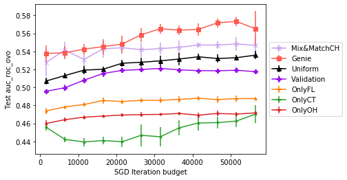
Figure 1: Test AUROC for predicting insurance plan for a mixture of FL, CT, and OH data

In this experiment, we split the Kaggle dataset into $K=3$ training datasets correspond to customer data from three states: Florida (FL), Connecticut (CT), and Ohio (OH). The validation and test datasets also consist of customers from these states, but the proportion of customers from various states is fixed. Details about the test and validation set formation is in the Appendix. In this case, $\boldsymbol{\alpha}^{*}$ is explicitly known for the Genie algorithm.

As shown in Figure 1, with respect to the AUROC metric, Mix&MatchCH is competitive with the Genie algorithm and has superior performance to all other baselines. The Validation algorithm has performance inferior to the uniform sampling scheme. Therefore, we are operating in a regime in which training on the validation set alone is not sufficient for good performance.

7.3 Amazon Employee Access Challenge:

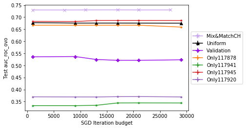
Figure 2: Test AUROC for predicting employee access in a new department, using training data from 4 departments

We evaluate our algorithms on the Amazon Employee Access Challenge Dataset Amazon, (2013). The goals is to whether or not the employee is allowed to access a resource given details about the employees role in the organization. We split the training data into different sources based on departments. The validation and test set has data from a new department unseen in the training data sources (In this case we don’t know $\boldsymbol{\alpha}^{*}$ explicitly to evaluate the Genie Algorithm). Additional details about the formation of datasets is in the Appendix.

We find that Mix&MatchCH outperforms the other baselines, and training solely on validation is insufficient to obtain a good AUROC score.

8 Acknowledgements

This work was partially supported by NSF Grant SATC 1704778, ARO grant W911NF-17-1-0359 and the WNCG Industrial Affiliated Program.

Appendix A A More Detailed Discussion on Prior Work

Transfer learning has assumed an increasingly important role, especially in settings where we are either computationally limited, or data-limited, and yet we have the opportunity to leverage significant computational and data resources yet on domains that differ slightly from the target domain Raina et al., (2007); Pan and Yang, (2009); Dai et al., (2009). This has become an important paradigm in neural networks and other areas Yosinski et al., (2014); Oquab et al., (2014); Bengio, (2011); Kornblith et al., (2018).

An important related problem is that of covariate shift Shimodaira, (2000); Zadrozny, (2004); Gretton et al., (2009). The problem here is that the target distribution may be different from the training distribution. A common technique for addressing this problem is by reweighting the samples in the training set, so that the distribution better matches that of the training set. There have been a number of techniques for doing this. An important recent thread has attempted to do this by using unlabelled data Huang et al., (2007); Gretton et al., (2009). Other approaches have considered a related problem of solving a weighted log-likelihood maximization Shimodaira, (2000), or by some form of importance sampling Sugiyama et al., (2007, 2008) or bias correction Zadrozny, (2004). In Mohri et al., (2019), the authors study a related problem of learning from different datasets, but provide mini-max bounds in terms of an agnostically chosen test distribution.

Our work is related to, but differs from all the above. As we explain in Section 3, we share the goal of transfer learning: we have access to enough data for training, but from a family of distributions that are different than the validation distribution (from which we have only enough data to validate). Under a model of covariate shift due to unobserved variables, we show that a target goal is finding an optimal reweighting of populations rather than data points. We use optimistic tree search to address precisely this problem – something that, as far as we know, has not been undertaken.

A key part of our work is working under a computational budget, and then designing an optimistic tree-search algorithm under uncertainty. We use a single SGD iteration as the currency denomination of our budget – i.e., our computational budget requires us to minimize the number of SGD steps in total that our algorithm computes. Enabling MCTS requires a careful understanding of SGD dynamics, and the error bounds on early stopping. There have been important SGD results studying early stopping, e.g., Hardt et al., (2015); Bottou et al., (2018) and generally results studying error rates for various versions of SGD and recentered SGD Nguyen et al., (2018); Defazio et al., (2014); Roux et al., (2012). Our work requires a new high probability bound, which we obtain in the Supplemental material, Section D. In Nguyen et al., (2018), the authors have argued that a uniform norm bound on the stochastic gradients is not the best assumption, however the results in that paper are in expectation. In this paper, we derive our SGD high-probability bounds under the mild assumption that the SGD gradient norms are bounded only at the optimal weight $\boldsymbol{w}^{*}$.

There are several papers Harvey et al., (2018); Rakhlin et al., (2012) which derive high probability bounds on the suffix averaged and final iterates returned by SGD for non-smooth strongly convex functions. However, both papers operate under the assumption of uniform bounds on the stochastic gradient. Although these papers do not directly report a dependence on the diameter of the space, since they both consider projected gradient descent, one could easily translate their constant dependence to a sum of a diameter dependent term and a stochastic noise term (by using the bounded gradient assumption from Nguyen et al., (2018), for example). However, as the set into which the algorithm would project is unknown to our algorithm (i.e., it would require knowing $\boldsymbol{w}^{*}$), we cannot use projected gradient descent in our analysis. As we see in later sections, we need a high-probability SGD guarantee which characterizes the dependence on diameter of the space and noise of the stochastic gradient. It is not immediately clear how the analysis in Harvey et al., (2018); Rakhlin et al., (2012) could be extended in this setting under the gradient bounded assumption in Nguyen et al., (2018). In Section 6, we instead develop the high probability bounds that are needed in our setting.

Optimistic tree search makes up the final important ingredient in our algorithm. These ideas have been used in a number of settings Bubeck et al., (2011); Grill et al., (2015). Most relevant to us is a recent extension of these ideas to a setting with biased search Sen et al., (2018, 2019).

Appendix B Standard Definitions from Convex Optimization

Recall that we assume throughout the paper that our loss functions satisfy the following assumptions similar to Nguyen et al., (2018):

Assumption 3 (Restated from main text).

For each loss function $f(\cdot;z)$ corresponding to a sample $z\in\mathcal{Z}$, we assume that $f(\cdot;z)$ is: (i) $\beta$-smooth (Definition 3) and (ii) convex (Definition 4).

Additionally, we assume that, for each $\boldsymbol{\alpha}\in\triangle$, the averaged loss function $F^{(\boldsymbol{\alpha})}(\cdot)$ is: (i) $\mu$-strongly convex (Definition 5) and (ii) $L$-Lipschitz (Definition 2).

We now state the definitions of these notions, which are standard in the optimization literature (see, for example, Bubeck, (2015)).

Definition 2 ($L$-Lipschitz).

We call a function $g(\cdot)$ $L$-Lipschitz if, for all $\boldsymbol{w},\boldsymbol{w}^{\prime}\in\mathcal{W}$,

$$|g(\boldsymbol{w})-g(\boldsymbol{w}^{\prime})|\leq L\|\boldsymbol{w}-\boldsymbol{w}^{\prime}\|_{2}.$$

Definition 3 ($\beta$-smooth).

We call a function $g(\cdot)$ $\beta$-smooth when, for all $\boldsymbol{w},\boldsymbol{w}^{\prime}\in\mathcal{W}$ when the gradient of $f$ is $\beta$-Lipschitz, i.e.,

$$\|\nabla g(\boldsymbol{w})-\nabla g(\boldsymbol{w}^{\prime})\|_{2}\geq\beta\|\boldsymbol{w}-\boldsymbol{w}^{\prime}\|_{2}.$$

Definition 4 (Convex).

We call a function $g(\cdot)$ convex when, for all $\boldsymbol{w},\boldsymbol{w}^{\prime}\in\mathcal{W}$,

$$g(\boldsymbol{w})\geq g(\boldsymbol{w}^{\prime})+\langle\nabla g(\boldsymbol{w}^{\prime}),\boldsymbol{w}-\boldsymbol{w}^{\prime}\rangle.$$

Definition 5 ($\mu$-strongly convex).

We call a function $g(\cdot)$ $\mu$-strongly convex if, for all $\boldsymbol{w},\boldsymbol{w}^{\prime}\in\mathcal{W}$,

$$g(\boldsymbol{w})\geq g(\boldsymbol{w}^{\prime})+\langle\nabla g(\boldsymbol{w}^{\prime}),\boldsymbol{w}-\boldsymbol{w}^{\prime}\rangle+\frac{\mu}{2}\|\boldsymbol{w}-\boldsymbol{w}^{\prime}\|_{2}^{2}.$$

Appendix C Smoothness with Respect to $\boldsymbol{\alpha}$

In this section we prove Theorem 1. The analysis is an interesting generalization of Theorem 3.9 in Hardt et al., (2015). The key technique is to create a total variational coupling between $\boldsymbol{\alpha}_{1}$ and $\boldsymbol{\alpha}_{2}$. Then using this coupling we prove that SGD iterates from the two distributions cannot be too far apart in expectation. Therefore, because the two sets of iterates converge to their respective optimal solutions, we can conclude that the optimal weights $\boldsymbol{w}^{*}(\boldsymbol{\alpha}_{1})$ and $\boldsymbol{w}^{*}(\boldsymbol{\alpha}_{2})$ are close.

Lemma 1.

Under conditions of Theorem 1, let $\boldsymbol{w}_{n}(\boldsymbol{\alpha}_{1})$ and $\boldsymbol{w}_{n}(\boldsymbol{\alpha}_{2})$ be the random variables representing the weights after performing $n$ steps of online projected SGD onto a convex body $\mathcal{X}=\mathrm{Conv}\{\boldsymbol{w}^{*}(\boldsymbol{\alpha})\mid\boldsymbol{\alpha}\in\mathcal{A}\}$ using the data distributions represented by the mixtures $\boldsymbol{\alpha}_{1}$ and $\boldsymbol{\alpha}_{2}$ respectively, starting from the same initial weight $\boldsymbol{w}_{0}$, and using the step size sequence described in Theorem 2. Then we have the following bound,

$$\mathbb{E}\left[\left\lVert\boldsymbol{w}_{n}(\boldsymbol{\alpha}_{1})-\boldsymbol{w}_{n}(\boldsymbol{\alpha}_{2})\right\rVert\right]\leq\frac{2\sigma\left\lVert\boldsymbol{\alpha}_{1}-\boldsymbol{\alpha}_{2}\right\rVert_{1}}{\mu}.$$

where $\sigma^{2}=\sup_{\boldsymbol{w},\boldsymbol{w}^{\prime}\in\mathcal{X}}\sup_{\boldsymbol{\alpha}\in\mathcal{A}}\beta^{2}\|\boldsymbol{w}-\boldsymbol{w}^{\prime}\|^{2}+\mathcal{G}_{*}(\boldsymbol{\alpha}).$

Proof.

We closely follow the proof of Theorem 3.9 in Hardt et al., (2015). Let $\boldsymbol{w}_{t+1}(\boldsymbol{\alpha}_{i})=\Pi_{\mathcal{X}}(\boldsymbol{w}_{t}-\eta_{t}\nabla f(\boldsymbol{w}_{t};Z^{(i)}_{t}))$ denote the SGD update while processing the $t$-th example from $\boldsymbol{\alpha}_{i}$ for $i\in\{1,2\}$. Let $I,J$ be two random variables whose joint distribution follows the variational coupling between $\boldsymbol{\alpha}_{1}$ and $\boldsymbol{\alpha}_{2}$. Thus the marginals of $I$ and $J$ are $\boldsymbol{\alpha}_{1}$ and $\boldsymbol{\alpha}_{2}$ respectively, while $\mathbb{P}(I\neq J)=d_{TV}(\boldsymbol{\alpha}_{1},\boldsymbol{\alpha}_{2})$. At each time $I_{t}\sim I$ and $J_{t}\sim J$ are drawn. If $I_{t}=J_{t}$, then we draw a data sample $Z_{t}$ from $D_{I_{t}}$ and set $Z^{(1)}_{t}=Z^{(2)}_{t}=Z_{t}$. Otherwise, we draw $Z^{(1)}_{t}$ from $D_{I_{t}}$ and $Z^{(2)}_{t}$ from $D_{J_{t}}$ independently.

Therefore, following the analysis in Hardt et al., (2015), if $I_{t}=J_{t}$, then, by Lemma 3.7.3 in Hardt et al., (2015), by our choice of step size, and since Euclidean projection does not increase the distance between projected points (see for example Lemma 3.1 in Bubeck, (2015)),

$$\delta_{t+1}^{2} =\|\boldsymbol{w}_{t+1}(\boldsymbol{\alpha}_{1})-\boldsymbol{w}_{t+1}(\boldsymbol{\alpha}_{2})\|^{2}$$

$$=\|\Pi_{\mathcal{X}}(\boldsymbol{w}_{t}(\boldsymbol{\alpha}_{1})-\eta_{t}\nabla f(\boldsymbol{w}_{t}(\boldsymbol{\alpha}_{1});Z_{t}))-\Pi_{\mathcal{X}}(\boldsymbol{w}_{t}(\boldsymbol{\alpha}_{2})-\eta_{t}\nabla f(\boldsymbol{w}_{t}(\boldsymbol{\alpha}_{2});Z_{t}))\|^{2}$$

$$\leq\|\boldsymbol{w}_{t}(\boldsymbol{\alpha}_{1})-\eta_{t}\nabla f(\boldsymbol{w}_{t}(\boldsymbol{\alpha}_{1});Z_{t})-\boldsymbol{w}_{t}(\boldsymbol{\alpha}_{2})+\eta_{t}\nabla f(\boldsymbol{w}_{t}(\boldsymbol{\alpha}_{2};Z_{t})\|^{2}$$

$$=\delta_{t}^{2}+\eta_{t}^{2}\|\nabla f(\boldsymbol{w}_{t}(\boldsymbol{\alpha}_{1});Z_{t})-\nabla f(\boldsymbol{w}_{t}(\boldsymbol{\alpha}_{2};Z_{t})\|^{2}$$

$$~{}~{}~{}~{}-2\eta_{t}\langle\nabla f(\boldsymbol{w}_{t}(\boldsymbol{\alpha}_{1});Z_{t})-\nabla f(\boldsymbol{w}_{t}(\boldsymbol{\alpha}_{2});Z_{t}),\boldsymbol{w}_{t}(\boldsymbol{\alpha}_{1})-\boldsymbol{w}_{t}(\boldsymbol{\alpha}_{2})\rangle$$

Now, taking expectations with respect to $Z_{t}$, we get the following:

$$\mathbb{E}_{Z_{t}}[\delta_{t+1}^{2}] \leq\delta_{t}^{2}+\eta_{t}^{2}\mathbb{E}_{Z_{t}}\|\nabla f(\boldsymbol{w}_{t}(\boldsymbol{\alpha}_{1});Z_{t})-\nabla f(\boldsymbol{w}_{t}(\boldsymbol{\alpha}_{2});Z_{t})\|^{2}$$

$$~{}~{}~{}~{}-2\eta_{t}\langle\nabla F(\boldsymbol{w}_{t}(\boldsymbol{\alpha}_{1}))-\nabla F(\boldsymbol{w}_{t}(\boldsymbol{\alpha}_{2})),\boldsymbol{w}_{t}(\boldsymbol{\alpha}_{1})-\boldsymbol{w}_{t}(\boldsymbol{\alpha}_{2})\rangle$$

$$\leq\delta_{t}^{2}+\eta_{t}^{2}\underbrace{\|\nabla f(\boldsymbol{w}_{t}(\boldsymbol{\alpha}_{1});Z_{t})-\nabla f(\boldsymbol{w}_{t}(\boldsymbol{\alpha}_{2};Z_{t})\|^{2}}_{\leq\beta^{2}\delta_{t}^{2}\text{ by smoothness of $f$}}$$

$$~{}~{}~{}~{}-2\eta_{t}\underbrace{\left(\frac{\mu\beta}{\mu+\beta}\|\boldsymbol{w}_{t}(\boldsymbol{\alpha}_{1})-\boldsymbol{w}_{t}(\boldsymbol{\alpha}_{2})\|^{2}+\frac{1}{\mu+\beta}\underbrace{\|\nabla F(\boldsymbol{w}_{t}(\boldsymbol{\alpha}_{1}))-\nabla F(\boldsymbol{w}_{t}(\boldsymbol{\alpha}_{2}))\|^{2}}_{\leq\mu^{2}\delta_{t}^{2}\text{by strong convexity of $F$}}\right)}_{\text{bound holds by Lemma 3.11 in \cite[cite]{\@@bibref{Authors Phrase1YearPhrase2}{bubeck15}{\@@citephrase{(}}{\@@citephrase{)}}}}}$$

$$=\left(1-2\eta_{t}\frac{\mu\beta}{\mu+\beta}\right)\delta_{t}^{2}-\eta_{t}\underbrace{\left(\frac{2\mu^{2}}{\mu+\beta}-\beta^{2}\eta_{t}\right)}_{\geq 0\text{ by choice of $\eta_{t}$}}\delta_{t}^{2}$$

$$\leq(1-\mu\eta_{t})\delta_{t}^{2}$$

where the last inequality follows since $\eta_{t}<\frac{\mu+\beta}{2\mu\beta}$, $\eta_{t}\leq\frac{2}{\kappa^{2}(\mu+\beta)}\leq\frac{1}{\mu\kappa^{2}},$ and $\beta\geq\mu.$ Thus, when $I_{t}=J_{t},$ we have that

$$\mathbb{E}_{Z_{t}}[\delta_{t+1}] \leq\sqrt{\mathbb{E}_{Z_{t}}[\delta_{t+1}^{2}]} \sqrt{.}$$ Using concavity of , and applying Jensen’s inequality

$$\leq\sqrt{(1-\mu\eta_{t})\delta_{t}^{2}}$$ using our bound above

$$\leq(1-\mu\eta_{t}/2)\delta_{t} \sqrt{1-\mu\eta_{t}}\leq 1-\frac{\mu\eta_{t}}{2}$$ since .

On the other hand, when $I_{t}\neq J_{t}$, we have that

$$\delta_{t+1} \leq\|\boldsymbol{w}_{t}(\boldsymbol{\alpha}_{1})-\eta_{t}\nabla f(\boldsymbol{w}_{t}(\boldsymbol{\alpha}_{1};Z^{(1)}_{t})-\boldsymbol{w}_{t}(\boldsymbol{\alpha}_{2})+\eta_{t}\nabla f(\boldsymbol{w}_{t}(\boldsymbol{\alpha}_{2};Z^{(2)}_{t}))\|$$

$$\leq\|\boldsymbol{w}_{t}(\boldsymbol{\alpha}_{1})-\eta_{t}\nabla f(\boldsymbol{w}_{t}(\boldsymbol{\alpha}_{1};Z^{(1)}_{t})-\boldsymbol{w}_{t}(\boldsymbol{\alpha}_{2})+\eta_{t}\nabla f(\boldsymbol{w}_{t}(\boldsymbol{\alpha}_{2};Z^{(1)}_{t})\|$$

$$~{}~{}~{}~{}+\eta_{t}(\|\nabla f(\boldsymbol{w}(\boldsymbol{\alpha}_{2});Z^{(1)})\|+\|\nabla f(\boldsymbol{w}(\boldsymbol{\alpha}_{2});Z^{(2)})\|)$$

$$\leq(1-\mu\eta_{t}/2)\delta_{t}+\eta_{t}(\|\nabla f(\boldsymbol{w}(\boldsymbol{\alpha}_{2});Z^{(1)})\|+\|\nabla f(\boldsymbol{w}(\boldsymbol{\alpha}_{2});Z^{(2)})\|)$$ By the previous bound

$$\leq(1-\mu\eta_{t}/2)\delta_{t}+\eta_{t}\sqrt{2\beta^{2}\|\boldsymbol{w}_{t}(\boldsymbol{\alpha}_{2})-\boldsymbol{w}^{*}(\boldsymbol{\alpha}_{1})\|^{2}+2\mathcal{G}_{*}(\boldsymbol{\alpha}_{1})}$$

$$~{}~{}~{}~{}+\eta_{t}\sqrt{2\beta^{2}\|\boldsymbol{w}_{t}(\boldsymbol{\alpha}_{2})-\boldsymbol{w}^{*}(\boldsymbol{\alpha}_{2})\|^{2}+2\mathcal{G}_{*}(\boldsymbol{\alpha}_{2})})$$ by Lemma 2

$$\leq(1-\mu\eta_{t}/2)\delta_{t}+2\sigma\eta_{t}$$

where $\sigma^{2}=\sup_{\boldsymbol{w},\boldsymbol{w}^{\prime}\in\mathcal{X}}\sup_{\boldsymbol{\alpha}\in\mathcal{A}}\beta^{2}\|\boldsymbol{w}-\boldsymbol{w}^{\prime}\|^{2}+\mathcal{G}_{*}(\boldsymbol{\alpha}).$

Thus, by combining both of these results, we obtain:

$$\mathbb{E}[\delta_{t+1}] \leq(1-\mu\eta_{t}/2)\mathbb{E}[\delta_{t}]+2\sigma\eta_{t}\mathbb{P}\{I_{t}\neq J_{t}\}$$

$$=(1-\mu\eta_{t}/2)\mathbb{E}[\delta_{t}]+\sigma\eta_{t}\left\lVert\boldsymbol{\alpha}_{1}-\boldsymbol{\alpha}_{2}\right\rVert_{1}.$$

Assuming that $\delta_{t_{0}}=0$, we get the following result from the recursion,

$$\mathbb{E}[\delta_{n}] \leq\sum_{t=t_{0}}^{n}\left\{\prod_{s=t+1}^{n}\left(1-\frac{1}{s+E}\right)\right\}\frac{2\sigma}{\mu(t+E)}\left\lVert\boldsymbol{\alpha}_{1}-\boldsymbol{\alpha}_{2}\right\rVert_{1}$$

$$=\sum_{t=t_{0}}^{n}\frac{t+E}{n+E}\frac{2\sigma}{\mu(t+E)}\left\lVert\boldsymbol{\alpha}_{1}-\boldsymbol{\alpha}_{2}\right\rVert_{1}$$

$$\leq\frac{n-t_{0}+1}{n+E}\frac{2\sigma}{\mu}\left\lVert\boldsymbol{\alpha}_{1}-\boldsymbol{\alpha}_{2}\right\rVert_{1}$$

$$\leq\frac{2\sigma}{\mu}\left\lVert\boldsymbol{\alpha}_{1}-\boldsymbol{\alpha}_{2}\right\rVert_{1}.$$

∎

Proof of Theorem 1.

First, note that by definition $\boldsymbol{w}^{*}(\boldsymbol{\alpha})$ is not a random variable i.e it is the optimal weight with respect to the distribution corresponding to $\boldsymbol{\alpha}$. On the other hand, $\boldsymbol{w}_{n}(\cdot)$ is a random variable, where the randomness is coming from the randomness in SGD sampling. By the triangle inequality, we have the following:

$$\left\lVert\boldsymbol{w}^{*}(\boldsymbol{\alpha}_{1})-\boldsymbol{w}^{*}(\boldsymbol{\alpha}_{2})\right\rVert \leq\left\lVert\boldsymbol{w}^{*}(\boldsymbol{\alpha}_{1})-{\boldsymbol{w}}_{n}(\boldsymbol{\alpha}_{1})\right\rVert+\left\lVert{\boldsymbol{w}}_{n}(\boldsymbol{\alpha}_{1})-{\boldsymbol{w}}_{n}(\boldsymbol{\alpha}_{2})\right\rVert+$$

$$\left\lVert\boldsymbol{w}^{*}(\boldsymbol{\alpha}_{2})-{\boldsymbol{w}}_{n}(\boldsymbol{\alpha}_{2})\right\rVert$$

$$\implies\left\lVert\boldsymbol{w}^{*}(\boldsymbol{\alpha}_{1})-\boldsymbol{w}^{*}(\boldsymbol{\alpha}_{2})\right\rVert =\mathbb{E}[\left\lVert\boldsymbol{w}^{*}(\boldsymbol{\alpha}_{1})-\boldsymbol{w}^{*}(\boldsymbol{\alpha}_{2})\right\rVert]$$

$$\leq\mathbb{E}[\left\lVert\boldsymbol{w}^{*}(\boldsymbol{\alpha}_{1})-{\boldsymbol{w}}_{n}(\boldsymbol{\alpha}_{1})\right\rVert]+\mathbb{E}[\left\lVert{\boldsymbol{w}}_{n}(\boldsymbol{\alpha}_{1})-{\boldsymbol{w}}_{n}(\boldsymbol{\alpha}_{2})\right\rVert]$$

$$+\mathbb{E}[\left\lVert\boldsymbol{w}^{*}(\boldsymbol{\alpha}_{2})-{\boldsymbol{w}}_{n}(\boldsymbol{\alpha}_{2})\right\rVert].$$ (9)

The expectation in the middle of the r.h.s. is bounded as in Lemma 1. We can use Theorem 2 in Nguyen et al., (2018) and Jensen’s inequality to bound the other two terms on the r.h.s. as

$$\mathbb{E}[\|{\boldsymbol{w}}_{n}(\boldsymbol{\alpha}_{1})-\boldsymbol{w}^{*}(\boldsymbol{\alpha}_{1})\|_{2}] \leq\sqrt{\mathbb{E}[\|{\boldsymbol{w}}_{n}(\boldsymbol{\alpha}_{1})-\boldsymbol{w}^{*}(\boldsymbol{\alpha}_{1})\|_{2}^{2}]} \sqrt{.}$$ by concavity of

$$\leq\sqrt{\frac{2\mathcal{G}_{*}G}{\mu^{2}(n+E)}}$$ by Theorem 2 in Nguyen et al., (2018)

where we take $\mathcal{G}_{*}=\max\{\mathcal{G}_{*}(\boldsymbol{\alpha}_{1}),\mathcal{G}_{*}(\boldsymbol{\alpha}_{2})\}$, $E$ is chosen as in Theorem 2, and $G=\max\left\{\frac{E\mu^{2}}{2\mathcal{G}_{*}},4\right\}.$ Now, noting that the inequality (9) holds for all $n$, we have the bound claimed in Theorem 1. ∎

Proof of Corollary 1.

This proof is a straightforward consequence of Theorem 3.1 in Kearfott, (1978) and Theorem 1. In particular, Theorem 3.1 in Kearfott, (1978) tells us that under the method of bisection of the simplex which they describe,

$$\|\boldsymbol{\alpha}_{1}-\boldsymbol{\alpha}_{2}\|_{2}\leq\left(\frac{\sqrt{3}}{2}\right)^{\lfloor\frac{h}{K-1}\rfloor}\text{diam}(\triangle),$$

where $\text{diam}(\triangle)=\sup\{\|\boldsymbol{\alpha}-\boldsymbol{\alpha}^{\prime}\|_{2}\mid\boldsymbol{\alpha},\boldsymbol{\alpha}^{\prime}\in\triangle\},$ and $K-1=\mathrm{dim}(\triangle).$ As noted in Remark 2.5 in Kearfott, (1978), $\text{diam}(\triangle)=\sqrt{2}$ since $\triangle$ is the unit simplex. Thus, by the Cauchy-Schwartz inequality, and since $\left\lfloor\frac{h}{K-1}\right\rfloor>\frac{h}{K-1}-1$, we have the following:

$$\|\boldsymbol{\alpha}_{1}-\boldsymbol{\alpha}_{2}\|_{1} \leq\sqrt{K}\|\boldsymbol{\alpha}_{1}-\boldsymbol{\alpha}_{2}\|_{2}$$

$$\leq\sqrt{2K}\left(\frac{\sqrt{3}}{2}\right)^{\lfloor\frac{h}{K-1}\rfloor}$$

$$\leq\sqrt{2K}\left(\frac{\sqrt{3}}{2}\right)^{\frac{h}{K-1}-1}.$$

Now we may use this result along with our assumption that $F$ is Lipschitz and Theorem 1 to obtain:

$$|G(\boldsymbol{\alpha}_{1})-G(\boldsymbol{\alpha}_{2})| =|F^{(te)}(\boldsymbol{w}^{*}(\boldsymbol{\alpha}_{1}))-F^{(te)}(\boldsymbol{w}^{*}(\boldsymbol{\alpha}_{2}))|$$

$$=|F^{(\boldsymbol{\alpha}^{*})}(\boldsymbol{w}^{*}(\boldsymbol{\alpha}_{1}))-F^{(\boldsymbol{\alpha}^{*})}(\boldsymbol{w}^{*}(\boldsymbol{\alpha}_{2}))|$$

$$\leq L\|\boldsymbol{w}^{*}(\boldsymbol{\alpha}_{1})-\boldsymbol{w}^{*}(\boldsymbol{\alpha}_{2})\|_{2}$$

$$\leq\frac{2L\sigma\|\boldsymbol{\alpha}_{1}-\boldsymbol{\alpha}_{2}\|_{1}}{\mu}$$

$$\leq\frac{4L\sigma\sqrt{2K}}{\sqrt{3}\mu}\left(\frac{\sqrt{3}}{2}\right)^{\frac{h}{K-1}},$$

which is the desired result. ∎

Appendix D New High-Probability Bounds on SGD without a Constant Gradient Bound

In this section, we will prove a high-probability bound on any iterate of SGD evolving over the time interval $t=1,2,\ldots,T,$ without assuming a uniform bound on the stochastic gradient over the domain. Instead, this bound introduces a tunable parameter $\Lambda>(T+1)$ that controls the trade-off between a bound on the SGD iterate $d_{t}^{2},$ and the probability with which the bound holds. As we discuss in Remark 5, this parameter can be set to provide tighter high-probability guarantees on the SGD iterates in settings where the diameter of the domain is large and/or cannot be controlled.

Theorem 2 (Restated from main text).

Consider a sequence of random samples $z_{0},z_{1},\ldots,z_{T}$ drawn from a distribution $p(z).$ Define the filtration $\mathcal{F}_{t}$ generated by $\sigma\{z_{0},z_{1},\ldots,z_{t}\}.$ Let us define a sequence of random variables by the gradient descent update: $\boldsymbol{w}_{t+1}=\boldsymbol{w}_{t}-\eta_{t}\nabla f(\boldsymbol{w}_{t};z_{t}),t=1,\ldots,T$, and $\boldsymbol{w}_{0}$ is a fixed vector in $\mathbb{R}^{d}.$

If we use the step size schedule $\eta_{t}=\frac{2}{\mu(t+E)},$ where $E=4096\kappa^{2}\log\Lambda^{8},$ then, under Assumptions 3 and 4, and taking $\Lambda\geq t+1$, we have the following high probability bound on the final iterate of the SGD procedure after $t$ time steps for any $k\geq 0$:

$$\mathrm{Pr}\left(d_{t+1}^{2}>\frac{G(d_{0}^{2},\mathcal{G}_{*})}{t+E+1}+\frac{8(t+1)\tilde{C}(D^{2},D\sqrt{\mathcal{G}_{*}})}{\mu(t+1+E)\Lambda^{7}}+\frac{4\sqrt{2\log(\Lambda^{8})}\sqrt{\hat{C}(k)}}{\mu(t+E+1)^{\alpha_{k+1}}}\right) \leq\frac{t+1}{\Lambda^{8}}$$ (10)

where

$$G(d_{0}^{2},\mathcal{G}_{*}) =\max\left\{Ed_{0}^{2},\frac{8\mathcal{G}_{*}}{\mu^{2}}\right\}$$

$$\tilde{C}(D^{2},D\sqrt{\mathcal{G}_{*}}) =D\sqrt{8\beta^{2}D^{2}+2\mathcal{G}_{*}}$$

$$\hat{C}(k) =O(\log\Lambda^{8})$$ See Corollary 3 for definition and Remark 6 for discussion.

$$\alpha_{k+1} =\sum_{i=1}^{k+1}\frac{1}{2^{i}}.$$

In particular, when we choose $k=0$, the above expression becomes

$$\mathrm{Pr}\left(d_{t+1}^{2}>\frac{G(d_{0}^{2},\mathcal{G}_{*})}{t+E+1}+\frac{8(t+1)\tilde{C}(D^{2},D\sqrt{\mathcal{G}_{*}})}{\mu(t+1+E)\Lambda^{7}}+\frac{4\sqrt{2\check{C}}\log(\Lambda^{8})}{\mu\sqrt{t+E+1}}\right) \leq\frac{t+1}{\Lambda^{8}}$$ (11)

where

$$\check{C} =\max\left\{\frac{8d_{0}^{2}(4\beta^{2}d_{0}^{2}+\mathcal{G}_{*})}{(1+E)\log\Lambda^{8}},\left(\frac{32\sqrt{2}\mathcal{G}_{*}}{\mu}+\frac{2}{E}\right)^{2},\left(\frac{64\beta^{2}c_{1}^{2}}{(1+E)\log\Lambda^{8}}+\frac{8\mathcal{G}_{*}c_{1}}{\log\Lambda^{8}}\right)^{2}\right\}$$

$$c_{1} =G(d_{0}^{2},\mathcal{G}_{*})+\frac{8\tilde{C}(D^{2},D\sqrt{\mathcal{G}_{*}})}{\mu\Lambda^{6}}$$

Remark 4.

This result essentially states that the distance of $\boldsymbol{w}_{t}$ to $\boldsymbol{w}^{*}$ is at most the sum of three terms with high probability. Recall from the first step of the proof of Theorem 2 in Nguyen et al., (2018) that $\mathbb{E}[d_{t}^{2}]\leq(1-\mu\eta_{t})\mathbb{E}[d_{t}^{2}]+2\eta_{t}^{2}\mathcal{G}_{*}+\mathbb{E}[M_{t}],$ where $M_{t}=\langle\nabla F(\boldsymbol{w}_{t})-\nabla f(\boldsymbol{w}_{t};z_{t}),\boldsymbol{w}_{t}-\boldsymbol{w}^{*}\rangle$ is a martingale difference sequence with respect to the filtration generated by samples $\boldsymbol{w}_{0},\ldots,\boldsymbol{w}_{t}$ (in particular, note that $\mathbb{E}[M_{t}]=0$). We obtain a similar inequality in the high probability analysis without the expectations, so bounding the $M_{t}$ term is the main difficulty in proving the high probability convergence guarantee. Indeed, the first term in our high-probability guarantee corresponds to a bound on the $(1-\mu\eta_{t})d_{t}+2\eta_{t}\mathcal{G}_{*}$ term. Thus, as in the expected value analysis from Nguyen et al., (2018), this term decreases linearly in the number of steps $t$, with the scaling constant depending only on the initial distance $d_{0}$ and a uniform bound on the stochastic gradient at the optimum model parameter ($\boldsymbol{w}^{*}$).

The latter two terms correspond to a bound on a normalized version of the martingale $\sum_{i}M_{i}$, which appears after unrolling the aforementioned recursion. Due to our more relaxed assumption on the bound on the norm of the stochastic gradient, we employ different techniques in bounding this term than were used in Harvey et al., (2018). The second term is a bias term that depends on the worst case diameter bound $D$ (or if no diameter bound exists, then $D$ represents the worst case distance between $\boldsymbol{w}_{t}$ and $\boldsymbol{w}^{*},$ see Remark 5), and appears as a result of applying Azuma-Hoeffding with conditioning. Our bound exhibits a trade-off between the bias term which is $O(D^{2}/\mathrm{poly}(\Lambda)),$ and the probability of the bad event which is $\frac{t+1}{\Lambda^{8}}.$ This trade-off can be achieved by tuning the parameter $\Lambda.$ Notice that while the probability of the bad event decays polynomially in $\Lambda,$ the bias only increases as $\mathrm{poly}(\log\Lambda).$

The third term represents the deviation of the martingale, which decreases nearly linearly in $t$ (i.e. $t^{\gamma}$ for any $\gamma$ close to $1$). The scaling constant, however, depends on $\gamma$. By choosing $\Lambda$ appropriately (in the second term), this third term decays the slowest of the three, for large values of $t,$ and is thus the most important one from a scaling-in-time perspective.

Remark 5.

In typical SDG analysis (e.g. Duchi et al., (2010); Harvey et al., (2018)), a uniform bound on the stochastic gradient is assumed. Note that if we assume a uniform bound on $d_{t}$, i.e. $d_{t}\leq D~{}\forall~{}t\in[1,T],$ then under Assumption 3, we immediately obtain a uniform bound on the stochastic gradient, since:

$$\|\nabla f(\boldsymbol{w}_{t};z)\| \leq\|\nabla f(\boldsymbol{w}_{t};z)-\nabla f(\boldsymbol{w}^{*};z)\|+\|\nabla f(\boldsymbol{w}^{*};z)\|$$

$$\leq\beta d_{t}+\sqrt{\mathcal{G}_{*}}$$

$$\leq\beta D+\sqrt{\mathcal{G}_{*}}:=\sqrt{\bar{\mathcal{G}}}$$ (12)

If we do not have access to a projection operator on our feasible set of $\boldsymbol{w},$ or otherwise choose not to run projected gradient descent, then we obtain a worst-case upper bound of $D=O\left(t^{u}\right)$ where $u=2\sqrt{2}\kappa^{3/2}$, since:

$$d_{t+1} \leq d_{t}+\eta_{t}\|\nabla f(\boldsymbol{w}_{t};z_{t})\|$$ by triangle inequality and definition of the SGD step

$$\leq d_{t}+\eta_{t}\sqrt{2\beta^{2}\kappa d_{t}^{2}+2\mathcal{G}_{*}}$$ by Lemma 2

$$\leq\left(1+\frac{\alpha\sqrt{2\kappa}\beta}{\mu(t+E)}\right)d_{t}+\frac{\alpha\sqrt{2\mathcal{G}_{*}}}{\mu(t+E)} \eta_{t}=\frac{\alpha}{\mu(t+E)} \alpha>1$$ by choice of , where must hold

$$=O\left(t^{\alpha\sqrt{2}\kappa^{3/2}}\right) \alpha=2$$ we take throughout this paper

Thus, when we do not assume access to the feasible set of $\boldsymbol{w}$ and do not run projected gradient descent, a convergence guarantee of the form $\tilde{O}\left(\frac{\bar{\mathcal{G}}}{t}\right)$ that follows from a uniform bound on the stochastic gradient does not suffice in our setting because $\bar{\mathcal{G}}$ scales polynomially in $t$. We further note that even if we do have access to a projection operator, $\bar{\mathcal{G}}$ scales quadratically in the radius of the projection set, and thus can be very large.

Instead, we wish to construct a high probability guarantee on the final SGD iterate in a fashion similar to the expected value guarantee given in Nguyen et al., (2018). Now under our construction, we have an additional parameter, $\Lambda,$ which we may use to our advantage to obtain meaningful convergence results even when $D$ scales polynomially. Indeed, we observe that each occurrence of $\tilde{C}$ in our construction is normalized by at least $\Lambda^{2}.$ Thus, since $\tilde{C}=O(D^{2}),$ by replacing $\Lambda\leftarrow\Lambda^{2u+1}$ in our analysis, and assuming $\Lambda$ is polynomial in $t,$ we can obtain (ignoring polylog factors) $\tilde{O}\left(\frac{1}{t^{\gamma}}\right)$ convergence of the final iterate of SGD, for any $\gamma<1$. Note that this change simply modifies the definition of $r_{t}$ by a constant factor. Thus, our convergence guarantee continues to hold with minor modifications to the choice of constants in our analysis.

A direct consequence of Theorem 2 and the fact that $\|\boldsymbol{w}_{0}-\boldsymbol{w}_{h+1,2i}^{*}\|_{2}^{2}\leq 2\|\boldsymbol{w}_{0}-\boldsymbol{w}_{h,i}\|_{2}^{2}+2\|\boldsymbol{w}_{h,i}^{*}-\boldsymbol{w}_{h+1,2i}\|_{2}^{2}\leq 4\nu_{1}\rho^{h}$ by Theorem 1 is the following Corollary, which guides our SGD budget allocation strategy.

Corollary 2.

Consider a tree node $(h,i)$ with mixture weights $\boldsymbol{\alpha}_{h,i}$ and optimal learning parameter $\boldsymbol{w}^{*}_{h,i}$. Assuming we start at a initial point $\boldsymbol{w}_{0}$ such that $\left\lVert\boldsymbol{w}_{0}-\boldsymbol{w}^{*}_{h,i}\right\rVert_{2}^{2}\leq\nu_{1}\rho^{h}$ and take $t=\lambda(h+1)$ SGD steps using the child node distribution $p^{(\boldsymbol{\alpha}^{*}_{h+1,2i})}$ where, $\lambda(h+1)$ is chosen to satisfy

$$\frac{G(4\nu_{1}\rho^{h},\mathcal{G}_{*})}{\lambda(h+1)+E}+\frac{8\lambda(h+1)\tilde{C}(D^{2},D\sqrt{\mathcal{G}_{*}})}{\mu(\lambda(h+1)+E)\Lambda^{7}}+\frac{4\sqrt{2\log(\Lambda^{8})}\sqrt{\hat{C}(k)}}{\mu(\lambda(h+1)+E)^{\alpha_{k+1}}}\leq\nu_{1}\rho^{h+1},$$ (13)

then by Theorem 2, with probability at least $1-\frac{1}{\Lambda^{7}}$ we have $||\boldsymbol{w}_{t}-\boldsymbol{w}^{*}_{h+1,2i}||_{2}^{2}\leq\nu_{1}\rho^{h+1}.$

In particular, if we assume that $D^{2}=K(t)d_{0}^{2}$ for some $K(t)$ such that $K(t)/\Lambda^{6}=\hat{K}=O(1)$ (refer to Remark 5 for why this particular assumption is reasonable), then when $G=Ed_{0}^{2}$ (i.e. $Ed_{0}^{2}\geq\frac{8\mathcal{G}_{*}}{\mu}$) and $\hat{C}(0)=\frac{8d_{0}^{2}(4\beta^{2}d_{0}^{2}+\mathcal{G}_{*})}{1+E}$ (note that a similar statement can be made if the third term inside the max in $\check{C}$ from Theorem 2, instead of the first term, is maximal), taking $k=0$, we may choose $\lambda(h)$ independently of $h$:

$$\lambda(h+1)=\lambda =\Bigg{(}\frac{1}{\rho\sqrt{1+E}}\bigg{(}4E+64\sqrt{2}\kappa\hat{K}+\frac{16\sqrt{E\hat{K}}}{\sqrt{\mu}\Lambda^{3}}$$

$$~{}~{}~{}~{}~{}~{}~{}~{}~{}~{}~{}~{}~{}~{}~{}~{}~{}~{}~{}~{}~{}~{}~{}~{}+128\kappa\sqrt{\log(\Lambda^{8})}+\frac{16\sqrt{2E\log(\Lambda^{8})}}{\sqrt{\mu}}\bigg{)}\Bigg{)}^{2}-E.$$ (14)

We will proceed in bounding the final iterate of SGD as follows:

• One main difficulty in analyzing the final iterate of SGD in our setting is our relaxed assumption on the norm of the gradient – namely, we assume that the norm of the gradient is bounded only at the optimal $\boldsymbol{w}^{*}.$ We thus will rely on Lemmas 2 and 3 to proceed with our analysis.

• In Lemmas 4 and 5, we will derive a bound on the distance from the optimal solution which takes a form similar to that in the expected value analysis of Nguyen et al., (2018); Bottou et al., (2018).

• Afterwards, we will define a sequence of random variables $r_{t}$ and $V_{t}$, in order to prove a high-probability result for $d_{t}^{2}>r_{t}$ in Lemma 8.

• Given this high probability result, it is then sufficient to obtain an almost sure bound on $r_{t}.$ We will proceed with bounding this quantity in several stages:

  • First, we obtain a useful bound on $r_{t}$ in Lemma 9 which normalizes the global diameter term $D$ by a term which is polynomial in our tunable parameter $\Lambda$. Note that this step is crucial to our analysis, as $D$ can potentially grow polynomially in the number of SGD steps $T$ under our assumptions, as we note in Remark 5.

  • Given this bound, we are left only to bound the $V_{t}$ term. We first obtain a crude bound on this term in Lemma 10, which would allow us to achieve a $\tilde{O}(1/\sqrt{t})$ converge guarantee. We then refine this bound in Corollary 3, which allows us to give a convergence guarantee of $\tilde{O}(K(\gamma)/t^{\gamma})$ for any $\gamma<1$ and for some constant $K(\gamma)$. We discuss how this refinement affects constant and $\log\Lambda$ factors in our convergence guarantee in Remark 6.

  • Finally, we collect our results to obtain our final bound on $r_{t+1}$ in Corollary 4.

• With a bound on $r_{t+1}$ and a high probability guarantee of $d_{t+1}$ exceeding $r_{t+1}$, we can finally obtain our high probability guarantee on error the final SGD iterate in Theorem 2.

Since quite a lot of notation will be introduced in this section, we provide a summary of parameters used here:

Parameter	Value	Description
$g(\boldsymbol{w}_{t};z_{t}),~{}g_{t}$	$\nabla f(\boldsymbol{w}_{t};z_{t})$	Interchangeable notation for stochastic gradient
$\kappa$	$\frac{\beta}{\mu}$	The condition number
$d_{t}$	$\|\boldsymbol{w}_{t}-\boldsymbol{w}^{*}\|_{2}^{2}$	The distance of the $t$th iterate of SGD
$\eta_{t}$	$\frac{2}{\mu(t+E)}$	The step size of SGD
$E$	$2048\kappa^{2}\log\Lambda^{4}$
$T$		The number of SGD iterations
$\Lambda$	$\geq T+1$	Tunable parameter to control high probability bound
$M_{t}$	$\langle\nabla F(\boldsymbol{w}_{t})-g_{t},\boldsymbol{w}_{t}-\boldsymbol{w}^{*}\rangle$
$\varrho_{t}$	$2d_{t}\sqrt{8\beta^{2}d_{t}^{2}+2\mathcal{G}_{*}}$	Upper bound on the martingale difference sequence
$D$	$\sup_{t=0,\ldots,T}d_{t}$	The uniform diameter bound (discussed in Remark 5)

We begin by noting that crucial to our analysis is deriving bounds on our stochastic gradient, since we assume the norm of the stochastic gradient is bounded only at the origin. The following results are the versions of Lemma 2 from Nguyen et al., (2018) restated as almost sure bounds.

Lemma 2 (Sample path version of Lemma 2 from Nguyen et al., (2018)).

Under Assumptions 3 and 4, the following bound on the norm of the stochastic gradient holds almost surely.

$$\|g(\boldsymbol{w}_{t},Z_{t})\|^{2}\leq 4\beta\kappa(F(\boldsymbol{w}_{t})-F(\boldsymbol{w}^{*}))+2\mathcal{G}_{*}$$ (15)

Proof.

As in Nguyen et al., (2018), we note that since

$$\|a-b\|^{2}\geq\frac{1}{2}\|a\|^{2}-\|b\|^{2},$$ (16)

we may obtain the following bound:

$$\frac{1}{2}\|\nabla f(\boldsymbol{w}_{t};z)\|^{2}-\|\nabla f(\boldsymbol{w}^{*};z)\|^{2} \leq\|\nabla f(\boldsymbol{w}_{t};z)-\nabla f(\boldsymbol{w}^{*};z)\|^{2}$$

$$\leq\beta^{2}\|\boldsymbol{w}_{t}-\boldsymbol{w}^{*}\|^{2} \beta f$$ by -smoothness of

$$\leq\frac{2\beta^{2}}{\mu}(F(\boldsymbol{w}_{t})-F(\boldsymbol{w}^{*})) \mu F$$ by -strong convexity of

Rearranging, we have that

$$\|\nabla f(\boldsymbol{w}_{t};z)\|^{2}\leq 4\beta\kappa(F(\boldsymbol{w}_{t})-F(\boldsymbol{w}^{*}))+2\mathcal{G}_{*},$$ (17)

as desired. ∎

Lemma 3 (Centered sample path version of Lemma 2 from Nguyen et al., (2018)).

Under Assumptions 3 and 4, for any random realization of $z$, the following bound holds almost surely:

$$\|\nabla f(\boldsymbol{w}_{t};z)-\nabla F(\boldsymbol{w}_{t})\|^{2}\leq 8\beta^{2}\|\boldsymbol{w}_{t}-\boldsymbol{w}^{*}\|^{2}+2\mathcal{G}_{*}$$ (18)

Proof.

The proof proceeds similarly to Lemma 2, replacing the stochastic gradient with the mean-centered version to obtain:

$$\frac{1}{2}\|\nabla f(\boldsymbol{w}_{t};z)-\mathbb{E}[\nabla f(\boldsymbol{w}_{t};z)]\|^{2}-\|\nabla f(\boldsymbol{w}^{*};z)-\mathbb{E}[\nabla f(\boldsymbol{w}^{*};z)]\|^{2}$$

$$\leq\|\nabla f(\boldsymbol{w}_{t};z)-\nabla f(\boldsymbol{w}^{*};z)-\mathbb{E}[\nabla f(\boldsymbol{w}_{t};z)]+\mathbb{E}[\nabla f(\boldsymbol{w}^{*};z)]\|^{2}$$

$$\leq 2(\|\nabla f(\boldsymbol{w}_{t};z)-\nabla f(\boldsymbol{w}^{*};z)\|^{2}+\|\mathbb{E}[\nabla f(\boldsymbol{w}_{t};z)]-\mathbb{E}[\nabla f(\boldsymbol{w}^{*};z)]\|^{2})$$

$$\leq 2(\|\nabla f(\boldsymbol{w}_{t};z)-\nabla f(\boldsymbol{w}^{*};z)\|^{2}+\mathbb{E}[\|\nabla f(\boldsymbol{w}_{t};z)-\nabla f(\boldsymbol{w}^{*};z)]\|^{2}])$$

$$\leq 4\beta^{2}\|\boldsymbol{w}_{t}-\boldsymbol{w}^{*}\|^{2}$$

Now, rearranging terms, and recalling that $\mathbb{E}[\nabla f(\boldsymbol{w}^{*};z)]=\nabla F(\boldsymbol{w}^{*})=0$, we have

$$\|\nabla f(\boldsymbol{w}_{t};z)-\nabla F(\boldsymbol{w}_{t};z)\|^{2} =\|\nabla f(\boldsymbol{w}_{t};z)-\mathbb{E}[\nabla f(\boldsymbol{w}_{t};z)]\|^{2}$$

$$\leq 8\beta^{2}\|\boldsymbol{w}_{t}-\boldsymbol{w}^{*}\|^{2}+2\|\nabla f(\boldsymbol{w}^{*};z)\|^{2}$$

$$\leq 8\beta^{2}\|\boldsymbol{w}_{t}-\boldsymbol{w}^{*}\|^{2}+2\mathcal{G}_{*}$$

as desired. ∎

Given these bounds on the norm of the stochastic gradient, we are now prepared to begin deriving high probability bounds on the optimization error of the final iterate.

Lemma 4.

Suppose $F$ and $f$ satisfy Assumptions 3 and 4. Consider the stochastic gradient iteration $\boldsymbol{w}_{t+1}=\boldsymbol{w}_{t}-\eta_{t}\nabla f(\boldsymbol{w}_{t};z_{t})$, where $z$ is sampled randomly from a distribution $p(z).$ Let $\boldsymbol{w}^{*}=\arg\min_{\boldsymbol{w}}F(\boldsymbol{w}).$ Let $M_{t}=\langle\nabla F(\boldsymbol{w}_{t})-g(\boldsymbol{w}_{t},Z_{t}),\boldsymbol{w}_{t}-\boldsymbol{w}^{*}\rangle,$ where $g(\boldsymbol{w},z)=\nabla f(\boldsymbol{w},z)$ . Additionally, let us adopt the notation $d_{t}=\|\boldsymbol{w}_{t}-\boldsymbol{w}^{*}\|_{2}$. Then the iterates satisfy the following inequality:

$$d_{t+1}^{2}\leq(1-\mu\eta_{t})d_{t}^{2}+2\mathcal{G}_{*}\eta_{t}^{2}+2\eta_{t}M_{t}$$ (19)

as long as $0<\eta_{t}\leq\frac{1}{2\beta\kappa}$, where $\kappa=\frac{\beta}{\mu}.$

Proof.

The proof crucially relies on techniques employed in Nguyen et al., (2018), and in particular, on Lemma 2, We now apply this result to bound $d_{t+1}:$

$$\|\boldsymbol{w}_{t+1}-\boldsymbol{w}^{*}\|^{2} =\|\boldsymbol{w}_{t}-\eta_{t}g(\boldsymbol{w}_{t};z_{t})-\boldsymbol{w}^{*}\|^{2}$$ by definition of SGD

$$=\|\boldsymbol{w}_{t}-\boldsymbol{w}^{*}\|^{2}+\eta_{t}^{2}\|g(\boldsymbol{w}_{t};z_{t})\|^{2}$$

$$~{}~{}~{}~{}-2\eta_{t}\langle g(\boldsymbol{w}_{t};z_{t}),\boldsymbol{w}_{t}-\boldsymbol{w}^{*}\rangle$$

$$\leq\|\boldsymbol{w}_{t}-\boldsymbol{w}^{*}\|^{2}+2\eta_{t}^{2}(\mathcal{G}_{*}+2\beta\kappa(F(\boldsymbol{w}_{t})-F(\boldsymbol{w}^{*})))$$

$$~{}~{}~{}~{}-2\eta_{t}(\langle\nabla F(\boldsymbol{w}_{t}),\boldsymbol{w}_{t}-\boldsymbol{w}^{*}\rangle$$

$$~{}~{}~{}~{}~{}~{}~{}~{}~{}~{}~{}~{}+\langle g_{t}-\nabla F(\boldsymbol{w}_{t}),\boldsymbol{w}_{t}-\boldsymbol{w}^{*}\rangle)$$ by Lemma 2

$$\leq\|\boldsymbol{w}_{t}-\boldsymbol{w}^{*}\|^{2}+2\eta_{t}^{2}(\mathcal{G}_{*}+2\beta\kappa(F(\boldsymbol{w}_{t})-F(\boldsymbol{w}^{*})))$$

$$~{}~{}~{}~{}-2\eta_{t}(F(\boldsymbol{w}_{t})-F(\boldsymbol{w}^{*})+\frac{\mu}{2}\|\boldsymbol{w}_{t}-\boldsymbol{w}^{*}\|^{2}$$

$$~{}~{}~{}~{}~{}~{}~{}~{}~{}~{}~{}~{}+\langle g_{t}-\nabla F(\boldsymbol{w}_{t}),\boldsymbol{w}_{t}-\boldsymbol{w}^{*}\rangle) \mu F$$ by -s.c. of

$$=(1-\mu\eta_{t})\|\boldsymbol{w}_{t}-\boldsymbol{w}^{*}\|^{2}$$

$$~{}~{}~{}~{}{\color[rgb]{0,0,1}-}2\eta_{t}(1-2\beta\kappa\eta_{t})(F(\boldsymbol{w}_{t})-F(\boldsymbol{w}^{*}))$$

$$~{}~{}~{}~{}-2\eta_{t}\langle g_{t}-\nabla F(\boldsymbol{w}_{t}),\boldsymbol{w}_{t}-\boldsymbol{w}^{*}\rangle+2\mathcal{G}_{*}\eta_{t}^{2}$$

$$\leq(1-\mu\eta_{t})d_{t}^{2}+2\mathcal{G}_{*}\eta_{t}^{2}+2\eta_{t}M_{t} \eta_{t}\leq\frac{1}{2\beta\kappa}$$ assuming

which is the desired result. ∎

Now given this recursion, we may derive a bound on $d_{t+1}$ in a similar form as expected value results from Theorem 2 from Nguyen et al., (2018) and Theorem 4.7 in Bottou et al., (2018). Namely,

Lemma 5.

Using the same assumptions and notation as in Lemma 4, by choosing $\eta_{t}=\frac{2}{\mu(t+E)}$, where $E\geq 4\kappa^{2}$ we have the following bound on the distance from the optimum:

$$d_{t}^{2} \leq\frac{G(d_{0}^{2},\mathcal{G}_{*})}{t+E}+\sum_{i=0}^{t-1}c(i,t-1)M_{i}$$

$$\leq\frac{G(d_{0}^{2},\mathcal{G}_{*})}{t+E}+\frac{4}{\mu(t+E)}\sum_{i=0}^{t}M_{i}$$

where

$$G(d_{0}^{2},\mathcal{G}_{*})=\max\{Ed_{0}^{2},\frac{8\mathcal{G}_{*}}{\mu^{2}}\},\text{ and }c(i,t)=2\eta_{i}\prod_{j=i+1}^{t}(1-\mu\eta_{j})$$

Proof.

We first note that our choice of $\eta_{t}$ does indeed satisfy $\eta_{t}\leq\frac{1}{2\beta\kappa},$ so we may apply Lemma 4.

As in the aforementioned theorems, our proof will proceed inductively.

Note that the base case of $t=0$ holds trivially by construction. Now let us suppose the bound holds for some $l<t.$ Then, using the recursion derived in Lemma 4, we have that

$$d_{l+1}^{2} \leq(1-\mu\eta_{l})d_{l}^{2}+2\mathcal{G}_{*}\eta_{t}^{2}+2\eta_{t}M_{t}$$

$$\leq(1-\mu\eta_{l})\left(\frac{G(d_{0}^{2},\mathcal{G}_{*})}{l+E}+\sum_{i=0}^{l-1}c(i,l-1)M_{i}\right)+2\mathcal{G}_{*}\eta_{l}^{2}+2\eta_{l}M_{l}$$

$$=(1-\mu\eta_{l})\frac{G(d_{0}^{2},\mathcal{G}_{*})}{l+E}+2\mathcal{G}_{*}\eta_{l}^{2}+\sum_{i=0}^{l}c(i,l)M_{i}$$

$$=G(d_{0}^{2},\mathcal{G}_{*})\frac{l+E-2}{(l+E)^{2}}+\frac{8\mathcal{G}_{*}}{\mu^{2}(l+E)^{2}}+\sum_{i=0}^{l}c(i,l)M_{i}$$

$$=G(d_{0}^{2},\mathcal{G}_{*})\frac{l+E-1}{(l+E)^{2}}-\frac{G(d_{0}^{2},\mathcal{G}_{*})}{(l+E)^{2}}+\frac{8\mathcal{G}_{*}}{\mu^{2}(l+E)^{2}}+\sum_{i=0}^{l}c(i,l)M_{i}$$

Now note that, by definition of $G(d_{0}^{2},\mathcal{G}_{*})$, we have that

$$-\frac{G(d_{0}^{2},\mathcal{G}_{*})}{(l+E)^{2}}+\frac{8\mathcal{G}_{*}}{\mu^{2}(l+E)^{2}}\leq 0$$ (20)

Therefore, we find that

$$d_{l+1}^{2} \leq G(d_{0}^{2},\mathcal{G}_{*})\frac{l+E-1}{(l+E)^{2}}+\sum_{i=0}^{l}c(i,l)M_{i}$$

$$=G(d_{0}^{2},\mathcal{G}_{*})\frac{(l+E)^{2}-1}{(l+E)^{2}}\frac{1}{t+E+1}+\sum_{i=0}^{l}c(i,l)M_{i}$$

$$\leq\frac{G(d_{0}^{2},\mathcal{G}_{*})}{(l+1)+E}+\sum_{i=0}^{l}c(i,l)M_{i}$$

Thus, the result holds for all $t.$

We now note that $c(i,t)\leq\frac{4}{\mu(t+E)}.$ Observe that

$$c(i,t) =2\eta_{i}\prod_{j=i+1}^{t}(1-\mu\eta_{j})$$

$$=\frac{4}{\mu(i+E)}\prod_{j=i+1}^{t}\frac{j+E-2}{j+E}$$

$$=\frac{4}{\mu(i+E)}\frac{i+E-1}{t+E}$$

$$\leq\frac{4}{\mu(t+E)}$$

∎

Now, in order to obtain a high probability bound on the final iterate of SGD, we need to obtain a concentration result for $\sum_{i=0}^{t}M_{i}.$ We note that, from Lemma 3, we obtain an upper bound on the magnitude of $M_{i}:$

$$|M_{t}| \leq\|g(\boldsymbol{w}_{t};z_{t})-\nabla F(\boldsymbol{w}_{t})\|\|\boldsymbol{w}_{t}-\boldsymbol{w}^{*}\|$$

$$\leq\sqrt{8\beta^{2}d_{t}^{2}+2\mathcal{G}_{*}}d_{t}.$$

We consider the usual filtration $\mathcal{F}_{t}$ that is generated by $\{z_{i}\}_{i\leq t}$ and $\mathbf{w}_{0}$. Just for completeness of notation we set $z_{0}=0$ (no gradient at step $0$).

By this construction, we observe that $M_{t}$ is a martingale difference sequence with respect to the filtration $\mathcal{F}_{t}$. In other words, $S_{t}=\sum_{s=1}^{t}M_{s}$ is a martingale.

Lemma 6.

$\mathbb{E}[M_{t}\mid\mathcal{F}_{t-1}]=0,~{}\forall t>0$.

Proof.

Given the filtration, $\mathcal{F}_{t-1}$, $\mathbf{w}_{0},z_{1}\ldots z_{t-1}$ is fixed. This implies that $\mathbf{w}_{t}$ is fixed. However, conditioned on $\{z_{i}\}_{i<t}$, $z_{t}$ is randomly sampled from $p(z)$. Therefore, $\mathbb{E}[g(\mathbf{w}_{t},z_{t})-\nabla F(\mathbf{w}_{t})\mid\mathcal{F}_{t-1}]=\mathbb{E}_{z_{t}\mid\mathcal{F}_{t-1}}[g(\mathbf{w}_{t},z_{t})-\nabla F(\mathbf{w}_{t})\mid\mathbf{w}_{t}]=\mathbb{E}_{z_{t}\sim p(z)}[g(\mathbf{w}_{t},z_{t})-\nabla F(\mathbf{w}_{t})\mid\mathbf{w}_{t}]=0$. Hence, $\mathbb{E}[M_{t}\mid\mathcal{F}_{t-1}]=0$ ∎

Recall that, $M_{s}$ is uniformly upper bounded by $\varrho_{t}=d_{t}\sqrt{8\beta^{2}d_{t}^{2}+2\mathcal{G}_{*}}$. Thus, we have that $\varrho_{t}^{2}\leq d_{t}^{2}(8\beta^{2}d_{t}^{2}+2\mathcal{G}_{*}).$

Let $D=\sup_{0\leq t\leq T}d_{t}$. Then, $|M_{t}|\leq d_{t}\sqrt{8\beta^{2}d_{t}^{2}+2\mathcal{G}_{*}}\leq\tilde{C}(D^{2},D\sqrt{\mathcal{G}_{*}})=D\sqrt{8\beta^{2}D^{2}+2\mathcal{G}_{*}}$.

In order to obtain a high probability bound on the final SGD iterate, we will introduce the following sequence of random variables and events, and additionally constants $c^{\prime}(t)$ to be decided later.

1. Initialization at $t=0$: Let $V_{0}=\frac{8d_{0}^{2}(4\beta^{2}d_{0}^{2}+\mathcal{G}_{*})}{1+E},$ $r_{0}=d_{0}^{2}$, and take $\mathcal{A}_{0}$ to be an event that is true with probability 1. Let $M_{0}=0$. $\mathrm{Pr}(\mathcal{E}_{0})$=1, $\delta_{0}=0$.

2. $r_{t}=\frac{G}{t+E}+\frac{4}{\mu(t+E)}(t-1)\delta_{t-1}\tilde{C}(D^{2},D\sqrt{\mathcal{G}_{*}})+\frac{4}{\mu}\sqrt{\frac{2\log(\Lambda^{8}/c^{\prime}(t))}{t+E}}\sqrt{V_{t-1}}$

3. $V_{t}=\frac{1}{t+E+1}\sum_{i=0}^{t}8r_{i}(4\beta^{2}r_{i}+\mathcal{G}_{*})$.

4. Event $\mathcal{A}_{t}$ is all sample paths satisfying the condition: $d_{t}^{2}\leq r_{t}$.

5. Let $\mathcal{E}_{t}=\bigcap_{i\leq t}\mathcal{A}_{i}$. Further, let $\mathrm{Pr}(\mathcal{E}^{c}_{t})/\mathrm{Pr}(\mathcal{E}_{t})=\delta_{t}.$

We now state a conditional form of the classic Azuma-Hoeffding inequality that has been tailored to our setting, and provide a proof for completeness.

Lemma 7 (Azuma-Hoeffding with conditioning).

Let $S_{n}=f(z_{1}\ldots z_{n})$ be a martingale sequence with respect to the filtration ${\cal F}_{n}$ generated by $z_{1}\ldots z_{n}$. Let $\psi_{n}=S_{n}-S_{n-1}$. Suppose $\lvert\psi_{n}\rvert\leq c_{n}(z_{1}\ldots z_{n-1})$ almost surely. Suppose $E[\psi_{n}\mid{\cal F}_{n-1}]=0$.

Let ${\cal A}_{n-1}$ be the event that $c_{n}\leq d_{n},$ where ${\cal A}_{n-1}$ is defined on the filtration ${\cal F}_{n-1},$ and $d_{n}$ is a constant dependent only on the index $n$. Define ${\cal E}_{n}=\bigcap_{i\leq n}{\cal A}_{i}$. Further suppose that that $\exists\bar{R}$ large enough such that $\lvert\psi_{n}\rvert\leq\bar{R}$ almost surely. Finally let $\mathrm{Pr}(\mathcal{E}^{c}_{n})/\mathrm{Pr}(\mathcal{E}_{n})=\delta_{n}.$ Then,

$$\mathrm{Pr}\left(S_{n}\geq\gamma+n\delta_{n}\bar{R}\ \lvert\ {\cal E}_{n}\right)\leq\exp\left(-\frac{\gamma^{2}}{2\sum_{i=1}^{n}d_{i}^{2}}\right)$$ (21)

Proof.

We first observe that $\mathbb{E}[\psi_{i}\mid{\cal F}_{i-1}]=0$. Therefore, for $i\leq n$ we have:

$$\lvert\mathbb{E}[\psi_{i}\mid\mathcal{E}_{n},{\cal F}_{i-1}]| =\frac{\mathrm{Pr}(\mathcal{E}_{n}^{c})}{\mathrm{Pr}(\mathcal{E}_{n})}|\mathbb{E}[\psi_{i}\mid\mathcal{E}_{n}^{c},{\cal F}_{i-1}]|$$

$$\leq\frac{\mathrm{Pr}(\mathcal{E}_{n}^{c})}{\mathrm{Pr}(\mathcal{E}_{n})}\bar{R}$$

$$\leq\delta_{n}\bar{R}$$ (22)

Consider the sequence $S^{\prime}_{i}=S_{i}-\sum_{j=1}^{i}\mathbb{E}[\psi_{j}\mid{\cal F}_{j-1},\mathcal{E}_{n}]$ for $i\leq n$.

$$\mathrm{Pr}(S^{\prime}_{i}\geq\gamma\mid\mathcal{E}_{n}) \leq e^{-\theta\gamma}\mathbb{E}[e^{\theta S^{\prime}_{i}}\mid\mathcal{E}_{n}]$$

$$=e^{-\theta\gamma}\mathbb{E}[\mathbb{E}[e^{\theta S^{\prime}_{i}}\mid\mathcal{E}_{n},{\cal F}_{i-1}]\mid\mathcal{E}_{n}]$$

$$=e^{-\theta\gamma}\mathbb{E}[e^{\theta S^{\prime}_{i-1}}\mathbb{E}[e^{\theta(\psi_{i}-\mathbb{E}[\psi_{i}\mid{\cal F}_{i-1},\mathcal{E}_{n}])}\mid\mathcal{E}_{n},{\cal F}_{i-1}]\mid\mathcal{E}_{n}]$$

Observe that $\mathbb{E}[\psi_{i}-\mathbb{E}[\psi_{i}\mid{\cal F}_{i-1},\mathcal{E}_{n}]\mid{\cal F}_{i-1},\mathcal{E}_{n}]=0$. i.e. $\psi_{i}-\mathbb{E}[\psi_{i}\mid{\cal F}_{i-1},\mathcal{E}_{n}]$ is a mean $0$ random variable with respect to the conditioning events ${\cal F}_{i-1},{\mathcal{E}}_{n}$.

Further, for any sample path where ${\mathcal{E}}_{n}$ holds, we almost surely have $\lvert\psi_{i}-\mathbb{E}[\psi_{i}\mid{\cal F}_{i-1},\mathcal{E}_{n}]\rvert\leq 2c_{i}(z_{1},z_{2}\ldots z_{i-1})\leq 2d_{i}.$

Therefore, $\mathbb{E}[e^{\theta(\psi_{i}-\mathbb{E}[\psi_{i}\mid{\cal F}_{i-1},\mathcal{E}_{n}])}\mid\mathcal{E}_{n},{\cal F}_{i-1}]\leq e^{4\theta d_{i}^{2}/2}$

Therefore, (D) yields the following:

$$\mathrm{Pr}(S^{\prime}_{i}\geq\gamma\mid\mathcal{E}_{n}) \leq e^{-\theta\gamma}\mathbb{E}[e^{\theta S^{\prime}_{i-1}}\mid\mathcal{E}_{n}][e^{\frac{4\theta d_{i}^{2}}{2}}]$$

$$=e^{-\theta\gamma}e^{\theta\sum_{j=1}^{i}4d_{j}^{2}/2}$$ (24)

Let $\theta=\frac{\gamma}{\sum_{i=1}^{n}4d_{i}^{2}}$. Then, we have for $i=n$:

$$\mathrm{Pr}\left(S_{n}\geq\gamma+\sum_{i=1}^{n}\mathbb{E}[\psi_{i}\mid{\cal F}_{i-1},\mathcal{E}_{i}]~{}\bigg{|}~{}{\cal E}_{n}\right)\leq\exp\left(-\frac{\gamma^{2}}{8\sum_{i=1}^{n}d_{i}^{2}}\right)$$

$$\overset{a}{\Rightarrow} \mathrm{Pr}\left(S_{n}\geq\gamma+n\delta_{n}\bar{R}\ \lvert\ {\cal E}_{n}\right)\leq\exp\left(-\frac{\gamma^{2}}{8\sum_{i=1}^{n}d_{i}^{2}}\right)$$ (25)

(a) - This is obtained by substituting the almost sure bound (D) for all $i\leq n$.

∎

Using our iterative construction and the conditional Azuma-Hoeffding inequality, we obtain the following high probability bound:

Lemma 8.

Under the construction specified above, we have the following:

$$\mathrm{Pr}(d_{t+1}^{2}>r_{t+1}\mid\mathcal{E}_{t}) \leq\frac{c^{\prime}(t+1)}{\Lambda^{8}}$$ (26)

When $c^{\prime}(i)=1$, we have:

$$\mathrm{Pr}(\mathcal{E}_{t+1}^{c})\leq\frac{t+1}{\Lambda^{8}}$$ (27)

Proof.

By the conditional Azuma-Hoeffding Inequality (Lemma 7), we have the following chain:

$$\mathrm{Pr}({\cal A}^{c}_{t+1}\lvert{\cal A}_{i},~{}i\leq t) {=\mathrm{Pr}(d_{t+1}^{2}>r_{t+1}\mid{\cal A}_{i},~{}i\leq t)}$$

$$\leq\mathrm{Pr}\Bigg{(}\frac{4}{\mu(t+1+E)}\sum_{i=1}^{t}(M_{i}-\delta_{t}\tilde{C}(D^{2},D\sqrt{\mathcal{G}_{*}}))>$$

$$~{}~{}~{}~{}~{}~{}~{}~{}~{}~{}~{}~{}\frac{4}{\mu(t+1+E)}\sqrt{\sum_{i=0}^{t}\varrho_{i}^{2}}\sqrt{2\log\left(\frac{\Lambda^{8}}{c^{\prime}(t+1)}\right)}~{}\bigg{|}~{}{\cal A}_{i},~{}i\leq t\Bigg{)}$$

$${\overset{a}{\leq}\exp\left(-\frac{(2\log(\frac{\Lambda^{8}}{c^{\prime}(t+1)}))\sum_{i=0}^{t}\varrho_{i}^{2}}{2\sum_{i=0}^{t}\varrho_{i}^{2}}\right)}$$

$$=\frac{c^{\prime}(t+1)}{\Lambda^{8}}$$

(a)- We set $\psi_{i}$ in Lemma 7 to be the variables $M_{i}$, filtrations ${\cal F}_{t}$ to be that generated by $z_{t}\sim p(z)$ (and $\mathbf{w}_{0}$) in the stochastic gradient descent steps. $c_{t}$ (in Lemma 7) set to $\varrho_{t}$, $d_{t}$ (in Lemma 7) is set to $r_{t}$ , $\bar{R}$ (in Lemma 7) is set to $\tilde{C}(D^{2},D\sqrt{\mathcal{G}_{*}})$ and $\delta_{t}$ (in Lemma 7) is set to $\mathrm{Pr}(\mathcal{E}^{c}_{t})/\mathrm{Pr}(\mathcal{E}_{t})$. Now, if we apply Lemma 7 to the sequence $M_{i}$ with the deviation $\gamma$ set to $\sqrt{\sum_{i=0}^{t}\varrho_{i}^{2}}\sqrt{2\log\left(\frac{\Lambda^{8}}{c^{\prime}(t+1)}\right)}$, we obtain the inequality.

$$\mathrm{Pr}(\mathcal{E}_{t+1}^{c}) \leq\sum_{i=1}^{t+1}\mathrm{Pr}(\min\{j:d_{j}^{2}>r_{j}\}=i)$$

$$\leq\sum_{i=1}^{t+1}\mathrm{Pr}(\mathcal{A}_{i}^{c}\mid{\cal A}_{j},~{}j<i)=\sum_{i=1}^{t+1}\frac{c^{\prime}(i)}{\Lambda^{8}}$$ (28)

Choosing $c^{\prime}(i)=1$, we thus obtain our desired result.

∎

From Lemma 8, we have a high probability bound on the event that $d_{t}^{2}>r_{t}.$ In order to translate this to a meaningful SGD convergence result, we will have to substitute for $\delta_{t}$. We thus upper bound $r_{t}$ as follows:

Lemma 9.

Under the above construction, where $c^{\prime}(i)$ is chosen to be $1$, we have the following almost sure upper bound on $r_{t},~{}\forall~{}t\leq\Lambda$

$$r_{t} \leq\frac{G(d_{0}^{2},\mathcal{G}_{*})}{t+E}+\frac{8t\tilde{C}(D^{2},D\sqrt{\mathcal{G}_{*}})}{\mu(t+E)\Lambda^{7}}+\frac{4\sqrt{2\log(\Lambda^{8})}\sqrt{V_{t-1}}}{\mu\sqrt{t+E}}$$ (29)

where $\tilde{C}(D^{2},D\sqrt{\mathcal{G}_{*}})=D\sqrt{8\beta^{2}D^{2}+2\mathcal{G}_{*}}$, and $D$ is taken to be a uniform diameter bound.

Proof.

From Lemma 8, we have: $\delta_{t}=\frac{\mathrm{Pr}(\mathcal{E}_{t}^{c})}{\mathrm{Pr}(\mathcal{E}_{t})}\leq\frac{t}{\Lambda^{8}-t}\leq\frac{2}{\Lambda^{7}}$. Here, we assume that $\Lambda>2$. Substituting in the expression for $r_{t}$, we have the result. ∎

Given this bound from Lemma 9, we now must construct an upper bound on $V_{t}.$ We will proceed in two steps, first deriving a crude bound on $V_{t}$, and then by iteratively refining this bound. We now derive the crude bound.

Lemma 10.

The following bound on $V_{t}$ holds almost surely:

$$V_{t}\leq\check{C}\log\Lambda^{8}$$ (30)

assuming that we choose

$$E \geq 128\beta^{2}c_{2}^{2}\log\Lambda^{8}$$

$$\check{C} \geq\max\left\{\frac{V_{0}}{\log\Lambda^{8}},(8\mathcal{G}_{*}c_{2}+\min\{2/E,1\})^{2},\left(\frac{64\beta^{2}c_{1}^{2}}{(1+E)\log\Lambda^{8}}+\frac{8\mathcal{G}_{*}c_{1}}{\log\Lambda^{8}}\right)^{2}\right\}$$

$$c_{1} =G(d_{0}^{2},\mathcal{G}_{*})+\frac{8\tilde{C}(D^{2},D\sqrt{\mathcal{G}_{*}})}{\mu\Lambda^{6}}$$

$$c_{2} =\frac{4\sqrt{2}}{\mu}$$

$$\Lambda \geq t+1$$

Proof.

We will prove the claim inductively.

We note that the base case when $t=0$ holds by construction, assuming that $\check{C}\geq\frac{V_{0}}{\log\Lambda^{4}}$.

Now let us suppose that our claim holds until some $t.$ Then by applying the bound on $r_{t}$ derived in Lemma 9, we have the following bound:

$$r_{t+1} \leq\frac{G(d_{0}^{2},\mathcal{G}_{*})}{t+1+E}+\frac{8(t+1)\tilde{C}(D^{2},D\sqrt{\mathcal{G}_{*}})}{\mu(t+1+E)\Lambda^{7}}+\frac{4\sqrt{2\check{C}}\log\Lambda^{8}}{\mu\sqrt{t+E+1}}$$

$$\leq\frac{c_{1}}{t+E+1}+\frac{c_{2}\sqrt{\check{C}}\log\Lambda^{8}}{\sqrt{t+E+1}},$$

where $c_{1}=G(d_{0}^{2},\mathcal{G}_{*})+\frac{8\tilde{C}(D^{2},D\sqrt{\mathcal{G}_{*}})}{\mu\Lambda^{6}}$ and $c_{2}=\frac{4\sqrt{2}}{\mu}$. Plugging in this bound to our definition of $V_{t+1},$ we obtain:

$$V_{t+1} =\frac{t+1+E}{t+2+E}V_{t}+32\beta^{2}r_{t+1}^{2}+8\mathcal{G}_{*}r_{t+1}$$

$$\leq\frac{\check{C}\log\Lambda^{8}}{t+E+2}\left((t+E+1)+\frac{64\beta^{2}c_{2}^{2}\log\Lambda^{8}}{t+E+1}+\frac{8\mathcal{G}_{*}c_{2}}{\sqrt{\check{C}(t+E+1)}}\right)$$

$$~{}~{}~{}~{}+\frac{1}{(t+E+1)(t+E+2)}\left(\frac{64\beta^{2}c_{1}^{2}}{(t+E+1)}+8\mathcal{G}_{*}c_{1}\right)$$

$$\overset{\mathrm{shown~{}below}}{\leq}\check{C}\log\Lambda^{8}$$

Rearranging, we find that we equivalently need:

$$\frac{64\beta^{2}c_{1}^{2}}{(t+E+1)\log\Lambda^{8}}+\frac{8\mathcal{G}_{*}c_{1}}{\log\Lambda^{8}} \leq\sqrt{\check{C}}(\sqrt{\check{C}}(t+E+1-64\beta^{2}c_{2}^{2}\log\Lambda^{8})$$

$$~{}~{}~{}~{}~{}~{}~{}~{}~{}~{}~{}~{}~{}~{}~{}~{}-8\mathcal{G}_{*}c_{2}\sqrt{t+E+1}).$$

Now, setting $E=2*64\beta^{2}c_{2}^{2}\log\Lambda^{8}$, we find that a sufficient condition to complete our induction hypothesis is:

$$\frac{64\beta^{2}c_{1}^{2}}{(t+E+1)\log\Lambda^{8}}+\frac{8\mathcal{G}_{*}c_{1}}{\log\Lambda^{8}} \leq\sqrt{\check{C}}((\sqrt{\check{C}}-4\mathcal{G}_{*}c_{2})(t+1)+(\sqrt{\check{C}}-8\mathcal{G}_{*}c_{2})E/2).$$ (31)

Now, observe that by choosing

$$\check{C}\geq\max\left\{(8\mathcal{G}_{*}c_{2}+\min\{2/E,1\})^{2},\left(\frac{64\beta^{2}c_{1}^{2}}{(1+E)\log\Lambda^{8}}+\frac{8\mathcal{G}_{*}c_{1}}{\log\Lambda^{8}}\right)^{2}\right\}$$ (32)

the sufficient condition (31) is satisfied. Hence, our claim holds for all $t$. ∎

Now given this crude upper bound, we may repeatedly apply Lemma 8 from Nguyen et al., (2018) in order to obtain the following result:

Corollary 3 (of Lemma 10 + Lemma 8 in Nguyen et al., (2018)).

After $k\geq 0$ applications of Lemma 8 from Nguyen et al., (2018), under the same assumptions as in Lemma 10, we have the following bound on $V_{t}:$

$$V_{t}\leq\frac{\hat{C}(k)}{(t+E+1)^{\alpha_{k}}}$$ (33)

where

$$\hat{C}(k+1) =2^{k+1}C(k+1)+V_{0}\frac{1+E}{(2+E)^{1-\alpha_{k+1}}}$$

$$C(k+1) =\frac{64\beta^{2}c_{1}^{2}}{(E+1)^{2-\alpha_{k+1}}}+\frac{64\hat{C}(k)c_{2}^{2}}{\mu^{2}(E+1)^{\alpha_{k+1}}}$$

$$~{}~{}~{}~{}+\frac{8\mathcal{G}_{*}c_{1}}{(E+1)^{1-\alpha_{k+1}}}+8\frac{\mathcal{G}_{*}}{\mu}\sqrt{\hat{C}(k)}c_{2}$$

$$\alpha_{k+1} =\sum_{i=1}^{k+1}\frac{1}{2^{i}}$$

$$\hat{C}(0) =\check{C}\log\Lambda^{8}$$

$$\alpha_{0} =0$$

where $E,\check{C},c_{1},c_{2}$ are defined as in Lemma 10.

Proof.

We will construct this bound inductively. We begin by noting that, when $k=0$, the bound holds by Lemma 10. Now let us assume the bound holds until some $k.$ Observe, then, that, by plugging into the bound in Lemma 9, we may write

$$V_{t+1}\leq\beta_{t}V_{t}+\gamma_{t}$$ (34)

where

$$\beta_{t} =\frac{t+1+E}{t+2+E}$$

$$\gamma_{t} =\frac{C(k+1)}{(t+E+1)^{\alpha_{k+1}}(t+E+2)}$$

$$C(k+1) =\frac{64\beta^{2}c_{1}^{2}}{(E+1)^{2-\alpha_{k+1}}}+\frac{64\hat{C}(k)c_{2}^{2}}{\mu^{2}(E+1)^{\alpha_{k+1}}}+\frac{8\mathcal{G}_{*}c_{1}}{(E+1)^{1-\alpha_{k+1}}}+8\frac{\mathcal{G}_{*}}{\mu}\sqrt{\hat{C}(k)}c_{2}$$

Now, we may apply Lemma 8 in Nguyen et al., (2018) to obtain:

$$V_{t+1} \leq\sum_{i=0}^{t}\left(\prod_{j=i+1}^{t}\beta_{j}\right)\gamma_{i}+V_{0}\prod_{i=0}^{t}\beta_{i}$$

$$=\sum_{i=0}^{t}\frac{i+2+E}{t+2+E}\frac{C(k+1)}{(i+E+1)^{\alpha_{k+1}}(i+E+2)}+V_{0}\frac{1+E}{t+2+E}$$

$$\leq\frac{C(k+1)}{t+2+E}\int_{E}^{t+1+E}\frac{1}{x^{\alpha_{k+1}}}dx+V_{0}\frac{1+E}{t+2+E}$$

$$\leq\frac{C(k+1)}{(1-\alpha_{k})(t+E+2)^{\alpha_{k+1}}}+V_{0}\frac{1+E}{t+E+2}$$

$$\leq\frac{\hat{C}(k+1)}{(t+E+2)^{\alpha_{k+1}}},$$

where $\hat{C}(k+1)=\frac{C(k+1)}{1-\alpha_{k+1}}+V_{0}\frac{1+E}{(2+E)^{1-\alpha_{k+1}}}=2^{k+1}C(k+1)+V_{0}\frac{1+E}{(2+E)^{1-\alpha_{k+1}}}$.

Thus, our claim holds for all $k.$ ∎

Remark 6.

Note that while $\hat{C}(k)$ in Corollary 3 has complicated dependencies on $\mathcal{G}_{*},$ $d_{0},$ $\beta$, and $\mu$, it is straightforward to argue that $\hat{C}(k)\leq\rho_{k}\log\Lambda^{8}$ where $\rho_{k}$ is a constant that is independent of $\Lambda$. Indeed, note that, from Corollary 3, we have that

$$\hat{C}(k+1) \leq 2^{k+1}\left[\frac{e_{1}}{(E+1)^{2-\alpha_{k+1}}}+\frac{e_{2}}{(E+1)^{1-\alpha_{k+1}}}+\frac{e_{3}}{(E+1)^{\alpha_{k+1}}}\hat{C}(k)+e_{4}\sqrt{\hat{C}(k)}\right]$$

$$~{}~{}~{}~{}+\frac{e_{5}}{(2+E)^{1-\alpha_{k+1}}}$$

for some $e_{1},\ldots,e_{5}$ which are independent of $\Lambda.$ Note that when $k=0$, the claimed bound on $\hat{C}(0)$ holds by definition, for proper choice of $\rho_{0}.$ Assuming the bound holds until $k,$ we may construct a bound of the desired form by choosing $\rho_{k+1}$ as a function of the $e_{i}$s. Note that $E+1\geq 1,$ and that each $e_{i}$ is independent of $\Lambda$, so $\rho_{k+1}$ is also independent of $\Lambda.$ We may thus conclude that $\hat{C}(k)=O(\log\Lambda^{8})$.

We may collect these results to obtain:

Corollary 4 (of Lemma 9 + Corollary 3).

Under the assumptions on $E$ in Lemma 10 and the definition of $\hat{C}(k)$ from Corollary 3, the following bound holds almost surely, for any $k\geq 0$,

$$r_{t+1} \leq\frac{G(d_{0}^{2},\mathcal{G}_{*})}{t+E+1}+\frac{8(t+1)\tilde{C}(D^{2},D\sqrt{\mathcal{G}_{*}})}{\mu(t+1+E)\Lambda^{7}}+\frac{4\sqrt{2\log(\Lambda^{8})}\sqrt{\hat{C}(k)}}{\mu(t+E+1)^{\sum_{i=1}^{k+1}2^{-i}}}$$ (35)

We are now prepared to state and prove our main SGD result.

Proof of Theorem 2.

The proof is an immediate consequence of Lemma 8 combined with Corollary 4. ∎

Appendix E Putting It Together: Tree-Search

Lemma 11.

With probability at least $1-\frac{1}{\Lambda^{3}}$, Algorithm 1 only expands nodes in the set $J:=\cup_{h=1}^{\Lambda}J_{h}$, where $J_{h}$ is defined as follows,

$$J_{h}:=\{\text{nodes }(h,i)\text{ such that }G(\boldsymbol{\alpha}_{h,i})-3\nu_{2}\rho_{2}^{h}\leq G(\boldsymbol{\alpha}^{*})\}.$$

Proof.

Let $A_{t}$ be the event that the leaf node that we decide to expand at time $t$ lies in the set $J$. Also let $\mathcal{L}_{t}$ be the set of leaf-nodes currently exposed at time $t$. Let $B_{t}=\bigcup_{(h,i)\in\mathcal{L}_{t}}\left\{\left\lVert\boldsymbol{w}_{h,i}-\boldsymbol{w}^{*}_{h,i}\right\rVert_{2}^{2}\leq\nu_{1}\rho^{h}\right\}.$

Now we have the following chain,

$$\mathbb{P}(B_{t}^{c}) =\mathbb{P}\left(\bigcup_{l=1}^{t/2}(\{B_{t}^{c}\}\cap\{|\mathcal{L}_{t}|=l\})\right)$$

$$\leq\sum_{l=1}^{t/2}\mathbb{P}\left(\{B_{t}^{c}\}\cap\{|\mathcal{L}_{t}|=l\}\right)$$

$$\leq\sum_{l=1}^{t/2}\mathbb{P}\left(\{B_{t}^{c}\}\right)$$

$$\stackrel{{\scriptstyle(a)}}{{\leq}}\sum_{l=1}^{t/2}\sum_{k=1}^{l}\frac{1}{\Lambda^{7}}$$

$$\leq\frac{1}{\Lambda^{5}}.$$

Here, $(a)$ is due to the h.p. result in Corollary 2. ∎

Now note that due to the structure of the algorithm an optimal node (partition containing the optimal point) at a particular height has always been evaluated prior to any time $t$, for $t\geq 2$. Now we will show that if $B_{t}$ is true, then $A_{t}$ is also true. Let the $\boldsymbol{\alpha}^{*}_{(h,i)}$ be a optimal node that is exposed at time $t$. Let $b^{*}_{h,i}$ be the lower confidence bound we have for that node. Therefore, given $B_{t}$ we have that,

$$b^{*}_{h,i} =F^{(te)}(\boldsymbol{w}_{h,i})-2\nu_{2}\rho_{2}^{h}$$

$$\leq G(\boldsymbol{\alpha}_{h,i})+L\left\lVert\boldsymbol{w}_{h,i}-\boldsymbol{w}^{*}(\boldsymbol{\alpha}_{h,i})\right\rVert_{2}-2\nu_{2}\rho_{2}^{h}$$

$$\leq G(\boldsymbol{\alpha}^{*})$$

So for a node at time $t$ to be expanded the lower confidence value of that node $b_{h,i}$ should be lower than $G(\boldsymbol{\alpha}^{*})$. Now again given $B_{t}$ we have that,

$$b_{h,i} =F^{(te)}(\boldsymbol{w}_{h,i})-2\nu_{2}\rho_{2}^{h}$$

$$\geq G(\boldsymbol{\alpha}_{h,i})-3\nu_{2}\rho_{2}^{h}.$$

Therefore, we have that $\mathbb{P}(A_{t}^{c})\leq\mathbb{P}(B_{t}^{c})$. Now, let $A$ be the event that over the course of the algorithm, no node outside of $J$ is every expanded. Let $T$ be the random variable denoting the total number of evaluations given our budget. We now have the following chain.

$$\mathbb{P}(A^{c}) =\mathbb{P}\left(\bigcup_{T=1}^{\Lambda}\left\{\bigcup_{t=1}^{T}\{A_{t}^{c}\}\right\}\cap\{T=l\}\right)$$

$$\leq\sum_{T=1}^{\Lambda}\mathbb{P}\left(\bigcup_{t=1}^{T}\{A_{t}^{c}\}\}\right)$$

$$\leq\frac{1}{\Lambda^{3}}$$

Lemma 12.

Let $h^{\prime}$ be the smallest number $h$ such that $\sum_{l=0}^{h}2C(\nu_{2},\rho_{2})\lambda(h)\rho_{2}^{-d(\nu_{2},\rho_{2})l}>\Lambda-2\lambda(h+1)$. The tree in Algorithm 1 grows to a height of at least $h(\Lambda)=h^{\prime}+1$, with probability at least $1-\frac{1}{\Lambda^{3}}$. Here, $\lambda(h)$ is as defined in Corollary 2.

Proof.

We have shown that only the nodes in $J=\cup_{h}J_{h}$ are expanded. Also, note that by definition $\lvert J_{h}\rvert\leq C(\nu_{2},\rho_{2})\rho_{2}^{-d(\nu_{2},\rho_{2})}$.

Conditioned on the event $A$ in Lemma 11, let us consider the strategy that only expands nodes in $J$, but expands the leaf among the current leaves with the least height. This strategy yields the tree with minimum height among strategies that only expand nodes in $J$. The number of s.g.d steps incurred by this strategy till height $h^{\prime}$ is given by,

$$\sum_{l=0}^{h^{\prime}}2C(\nu_{2},\rho_{2})\lambda(l)\rho_{2}^{-d(\nu_{2},\rho_{2})l}.$$

Since the above number is greater than to $\Lambda-2\lambda(h^{\prime}+1)$ another set of children at height $h^{\prime}+1$ is expanded and then the algorithm terminates because of the check in the while loop in step 4 of Algorithm 1. Therefore, the resultant tree has a height of at least $h^{\prime}+1$. ∎

Proof of Theorem 3.

Given that event $A$ in Lemma 11 holds, Lemma 12 shows that at least one node at height $h^{\prime}$ (say $(h^{\prime},i)$) is expanded and one of that node’s children say $\boldsymbol{\alpha}_{h^{\prime}+1,i^{\prime}}$ is returned by the algorithm. Note that $(h^{\prime},i)$ is in $J_{h}$ and therefore $G(\boldsymbol{\alpha}_{h^{\prime},i})-3\nu_{2}\rho_{2}^{h^{\prime}}\geq G(\boldsymbol{\alpha}^{*})$. Invoking the smoothness property in Corollary 1, we get that

$$G(\boldsymbol{\alpha}_{h^{\prime}+1,i^{\prime}})\leq G(\boldsymbol{\alpha}^{*})+4\nu_{2}\rho_{2}^{h^{\prime}}.$$ (36)

∎

Appendix F Scaling of $h(\Lambda)$ and $\lambda(h)$

In this section, we discuss how to interpret the scaling of the height function $h(\Lambda)$ from Theorem 3 and the SGD budget allocation strategy $\lambda(h)$ from Corollary 2.

Let us take $k=0$ in Theorem 2, and assume the third term in the high probability bound is dominant: that is, for some constant $K$ large enough, taking $C=\frac{4\sqrt{2\check{C}}K\log\Lambda^{8}}{\mu}$, we want to choose $\lambda(h)$ to satisfy:

$$\frac{C\log\Lambda}{\sqrt{\lambda(h)+E}}\leq\nu_{1}\rho^{h+1}.$$ (37)

Then, solving for $\lambda(h)$, we have that

$$\lambda(h) =\left(\frac{C\log\Lambda}{\nu_{1}\rho^{h+1}}\right)^{2}-E$$ (38)

$$=\tilde{O}\left(\frac{1}{\rho^{2h}}\right)$$ (39)

Thus, outside of the constant scaling regime discussed in Corollary 2, we expect SGD to take an exponential (in height) number of SGD steps in order to obtain a solution that is of distance $\nu_{1}\rho^{h+1}$ from the optimal solution w.h.p. (Recall that $\rho\in(0,1)$)

In light of this, we may discuss now how the depth of the seach tree, $h(\Lambda)$, scales as a function of the total SGD budget $\Lambda$. We will let

$$\lambda(h)=\begin{cases}\lambda_{const}&\text{When $h$ is in constant step size regime}\\ \frac{C^{\prime}\log^{2}\Lambda}{\nu_{1}\rho^{2h}}&\text{Outside of this regime, for $C^{\prime}$ chosen large enough}\end{cases}$$ (40)

We may thus solve for $h^{\prime}$ from Theorem 3 as follows. Denote $h_{const}$ as the maximum height of the tree for which $\lambda(h)=\lambda_{const}$ for all $h\leq h_{const}$. Then:

$$\sum_{i=0}^{h(\Lambda)-1}2C(\nu_{2},\rho_{2})\lambda(l)\rho^{-d(\nu_{2},\rho_{2})l} =2C(\nu_{2},\rho_{2})\lambda_{const}\sum_{i=0}^{h_{const}}\rho^{-d(\nu_{2},\rho_{2})l}+2\tilde{C}\log^{2}\Lambda\sum_{l=h_{const}+1}^{h(\Lambda)-1}\rho^{-(d(\nu_{2},\rho_{2})+2)l}$$

$$=\underbrace{2C(\nu_{2},\rho_{2})\lambda_{const}\frac{\rho^{-d(\nu_{2},\rho_{2})(h_{const}+1)}-1}{\rho^{-d(\nu_{2},\rho_{2})}-1}}_{T1}$$

$$~{}~{}~{}~{}+\underbrace{2\tilde{C}\log^{2}\Lambda\frac{\rho^{-(d(\nu_{2},\rho_{2})+2)h(\Lambda)}-\rho^{-(d(\nu_{2},\rho_{2})+2)(h_{const}+2)}}{\rho^{-(d(\nu_{2},\rho_{2})+2)}-1}}_{T2}$$

$$\overset{want}{>}\Lambda-2\lambda(h(\Lambda))$$

Now, observe that when $h_{const}=h(\Lambda)$, then $T2=0$, and we need that, solving for $h_{const}$,

$$h(\Lambda)>\frac{1}{d(\nu_{2},\rho_{2})}\log_{\frac{1}{\rho}}\left(\frac{\rho^{-d}-1}{2C(\nu_{2},\rho_{2})\lambda_{const}}(\Lambda-2\lambda_{const})+1\right)$$

and thus, $h(\Lambda)=h_{const}$ scales as $O(\log_{\frac{1}{\rho}}\Lambda)$ w.h.p.

When $\Lambda$ is sufficiently large so that $h(\Lambda)>h_{const}$ and $h_{const}$ can be taken as a constant, we need that, for a sufficiently large constant $\hat{C}$,

$$\hat{C}\log^{2}\Lambda\frac{\rho^{-(d(\nu_{2},\rho_{2})+2)h(\Lambda)}-\rho^{-(d(\nu_{2},\rho_{2})+2)(h_{const}+2)}}{\rho^{-(d(\nu_{2},\rho_{2})+2)}-1} \overset{want}{>}\Lambda-2\frac{C\log^{2}\Lambda}{\nu_{1}\rho^{2h(\Lambda)}}$$

Solving for $h(\Lambda)$, we find that, for some large enough constant $\hat{\hat{C}}$, we must have that

$$h(\Lambda)>\frac{1}{d(\nu_{2},\rho_{2})+2}\left(\log_{\frac{1}{\rho}}\frac{\Lambda}{\hat{\hat{C}}\log^{2}\Lambda}\right)$$

and thus, in this case, $h(\Lambda)$ scales as $O\left(\log_{\frac{1}{\rho}}\frac{\Lambda}{\log^{2}\Lambda}\right)$ w.h.p.

In the context of Theorem 3, this scaling shows that the simple regret of our algorithm, $R(\Lambda)$, scales roughly as $\tilde{O}\left(\frac{1}{\Lambda^{c}}\right)$ for some constant $c$. Thus, in certain small validation set regimes as discussed in Remark 1, Mix&Match gives an exponential improvement in simple regret compared to an algorithm which trains only on the validation dataset.

Appendix G Additional Experimental Details

G.1 Details about the experimental setup

All experiments were run in python:3.7.3 Docker containers (see https://hub.docker.com/_/python) managed by Google Kubernetes Engine running on Google Cloud Platform on n1-standard-4 instances. Hyperparameter tuning is performed using the Katib framework (https://github.com/kubeflow/katib) using the validation error as the objective. The code used to create the testing infrastructure can be found at https://github.com/matthewfaw/mixnmatch-infrastructure, and the code used to run experiments can be found at https://github.com/matthewfaw/mixnmatch.

G.2 Details about the multiclass AUC metric

We briefly discuss the AUC metric used throughout our experiments. We evaluate each of our classification tasks using the multi-class generalization of area under the ROC curve (AUROC) proposed by Hand and Till, (2001). This metric considers each pair of classes (i,j), and for each pair, computes an estimate for the probability that a random sample from class $j$ has lower probability of being labeled as class $i$ than a random sample from class $j$. The metric reported is the average of each of these pairwise estimates. This AUC genenralization is implemented in the R pROC library https://rdrr.io/cran/pROC/man/multiclass.html, and also in the upcoming release of sklearn 0.22.0 https://github.com/scikit-learn/scikit-learn/pull/12789. In our experiments, we use the sklearn implementation.

G.3 Description of algorithms used

In the sections that follow, we will reference the following algorithms considered in our experiments. We note that the algorithms discussed in this section are a superset of those discussed in Section 7.

Table 1: Description of the algorithms used in the experiments

Algorithm ID	Description
Mix&MatchCH	The Mix&Match algorithm, where the simplex is partitioned using a random coordinate halving scheme
Mix&MatchDP	The Mix&Match algoirhtm, where the simplex is partitioned using the Delaunay partitioning scheme
Mix&MatchCH+0.1Step	Runs the Mix&MatchCH algorithm for the first half of the SGD budget, and runs SGD sampling according to the mixture returned by Mix&Match for the second half of the SGD budget, using a step size 0.1 times the size used by Mix&Match
Mix&MatchDP+0.1Step	Runs the Mix&MatchDP algorithm for the first half of the SGD budget, and runs SGD sampling according to the mixture returned by Mix&Match for the second half of the SGD budget, using a step size 0.1 times the size used by Mix&Match
Genie	Runs SGD, sampling from the training set according to the test set mixture
Validation	Runs SGD, sampling only from the validation set according to the test set mixture
Uniform	Runs SGD, sampling uniformly from the training set
OnlyX	Runs SGD, sampling only from dataset X

G.4 Allstate Purchase Prediction Challenge – Correcting for shifted mixtures

Here, we provide more details about the experiment on the Allstate dataset Allstate, (2014) discussed in Section 7. Recall that in this experiment, we consider the mixture space over which Mix&Match searches to be the set of mixtures of data from Florida (FL), Connecticut (CT), and Ohio (OH). We take $\boldsymbol{\alpha}^{*}$ to be the proportion of each state in the test set. The breakdown of the training/validation/test split for the Allstate experiment is shown in Table 2.

Table 2: The proportions of data from each state used in training, validation, and testing for Figure 1 and 3

State	Total Size	% Train	% Validate	% Test	% Discarded
FL	14605	49.34	0.16	0.5	50
CT	2836	50	7.5	42.5	0
OH	6664	2.25	0.75	2.25	94.75

Here, each Mix&Match algorithm allocates a height-independent 500 samples for each tree search node on which SGD is run. Each algorithm uses a batch size of 100 to compute stochastic gradients.

G.4.1 Dataset transformations performed

We note that in the dataset provided by Kaggle, the data for a single customer is spread across multiple rows of the dataset, since for each customer there some number (different for various customers) of intermediate transactions, followed by a row corresponding to the insurance plan the customer ultimately selected. We collapse the dataset so that each row corresponds to the information of a distinct customer. To do this, for each customer, we preserve the final insurance plan selected, the penultimate insurance plan selected in their history, the final and penultimate cost of the plan. Additionally, we create a column indicating the total number of days the customer spent before making their final transaction, as well as a column indicating whether or not a day elapsed between intermediate and final purchase, a column indicating whether the cost of the insurance plan changed, and a column containing the price amount the insurance plan changed between the penultimate and final purchase. For every other feature, we preserve only the value in the row corresponding to the purchase. We additionally one-hot encode the car_value feature. Additionally, we note that we predict only one part of the insurance plan (the G category, which takes 4 possible values). We keep all other parts of the insurance plan as features.

G.4.2 Experimental results

Figure 3 shows the results of the same experiment as discussed in Section 7. We note that there are now several variants of the Mix&Match algorithm, whose implementations are described in Table 1. We observe that, in this experiment, the two simplex partitioning schemes result in algorithms that all have similar performance on the test set, and each instance of Mix&Match outperforms algorithms which train only on a single state’s training set as well as the algorithm which trains only on the validation dataset, which is able to sample using the same mixture as the test set, but with limited amounts of data. Additionally, each instance of Mix&Match has either competitive or better performance than the Uniform algorithm, and has performance competitive with the Genie algorithm.

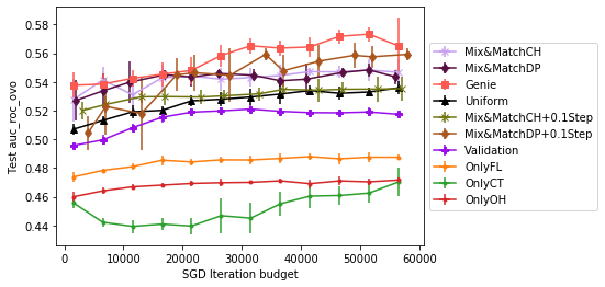
Figure 3: Test One vs One AUROC for Mixture of FL, CT, and OH

G.5 Wine Ratings

We consider the effectiveness of using Algorithm 1 to make predictions on a new region by training on data from other, different regions. For this experiment, we use another Kaggle dataset Bahri, (2018), in which we are provided binary labels indicating the presence of particular tasting notes of the wine, as well as a point score of the wine and the price quartile of the wine, for a number of wine-producing countries. We will consider several different experiments on this dataset.

We will consider again algorithms discussed in Table 1. Throughout these experiments, we will consider searching over the mixture space of proportions of datasets of wine from countries US, Italy, France, and Spain. Note that the Genie experiment is not run since there is no natural choice for $\boldsymbol{\alpha}^{*},$ as we are aiming to predict on a new country.

G.5.1 Dataset transformations performed

The dataset provided through Kaggle consists of binary features describing the country of origin of each wine, as well as tasting notes, and additionally a numerical score for the wine, and the price. We split the dataset based on country of origin (and drop the country during training), and add as an additional target variable the price quartile. We keep all other features in the dataset. In the experiment predicting wine prices, we drop the price quartile column, and in the experiment predicting wine price quartiles, we drop the price column.

G.5.2 Predict wine prices

In this section, we consider the task of predicting wine prices in Chile and Australia by using training data from US, Italy, France, and Spain. The train/validation/test set breakdown is described in Table 3. We use each considered algorithm to train a fully connected neural network with two hidden layers and sigmoid activations, similarly as considered in Zhao et al., (2018). We plot the test mean absolute error of each considered algorithm.

Here, each Mix&Match algorithm allocates a height-independent 500 samples for each tree search node on which SGD is run. Each algorithm uses a batch size of 25 to compute stochastic gradients.

Table 3: The proportions of data from each state used in training, validation, and testing for Figure 4

Country	Total Size	% Train	% Validate	% Test	% Discarded
US	54265	100	0	0	0
France	17776	100	0	0	0
Italy	16914	100	0	0	0
Spain	6573	100	0	0	0
Chile	4416	0	5	95	0
Australia	2294	0	5	95	0

The results of this experiment are shown in Figure 4. There are several interesting takeaways from this experiment. First is the sensitivity of Mix&Match to choice of partitioning scheme. While Mix&MatchCH outperforms the Uniform algorithm and each OnlyX algorithm, Mix&MatchDP performs poorly. Note that each node in the search tree under Delaunay partitioning can have $dim(\mathcal{A})$ ($=4$ in this experiment) children, each node in the coordinate halving scheme only has two children. Thus, it seems that perhaps the Dealunay partitioning scheme is overly wasteful in its allocation of SGD budget. However, when considering the split budget Mix&Match algorithms which search for mixtures only for half of their SGD budget, and commit to a mixture for the remaining half, the performance gap between the two partitioning schemes is much less noticeable.

The second interesting takeaway from this experiment is that, in contrast to the other experiments considered in this paper, in this experiment, it seems that although Mix&Match outperforms both the Uniform algorithm and OnlyX algorithm, it only matches the performance of the algorithm which trains only on the validation dataset. This highlights an important point of the applicability of the Mix&Match algorithm. Running Mix&Match makes sense only when there is insufficient validation data to train a good model.

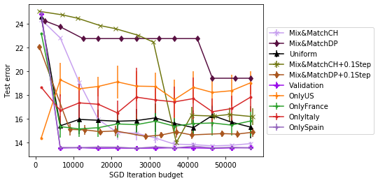
Figure 4: Test Mean Absolute Error for Mixture of US, France, Italy, and Spain data, Predict in Chile and Australia

G.5.3 Predict wine price quartiles

In this experiment, we consider a classification version of the regression problem considered in the last experiment. In particular, we have access to training wine data from US, Italy, Spain, and France, and wish to predict the quartile of the wine price for wines from Chile. The train/validate/test breakdown in given in Table 4. We use each algorithm to train a fully connected neural network with 3 hidden layers and ReLU activations, and evaluate based on the One vs One AUROC metric described in Hand and Till, (2001). The experimental results are shown in Figure 5

Here, each Mix&Match algorithm allocates a height-independent 1000 samples for each tree search node on which SGD is run. Each algorithm uses a batch size of 25 to compute stochastic gradients.

Table 4: The proportions of data from each state used in training, validation, and testing for Figure 5

Country	Total Size	% Train	% Validate	% Test	% Discarded
US	54265	100	0	0	0
France	17776	100	0	0	0
Italy	16914	100	0	0	0
Spain	6573	100	0	0	0
Chile	4416	0	5	95	0

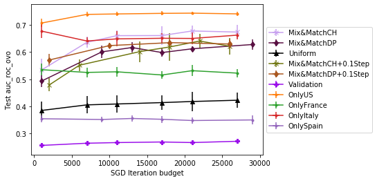
Figure 5: Test One vs One AUROC for Mixture of US, France, Italy, and Spain data, Predict in Chile

We observe that each instance of Mix&Match outperforms both Uniform and Validation (which has quite poor performance in this experiment), and has competitive performance with the best OnlyX algorithm.

G.6 Amazon Employee Access Challenge

Here, we consider yet another Kaggle dataset, the Amazon Employee Access Challenge Amazon, (2013). In this problem, we are given a dataset of features about employees from a variety of departments, and we wish to predict whether or not a employee is granted access to the system. We note that this dataset is extremely imbalanced, as most requests are approved.

We split this dataset according to department names, with splits shown in Table 5. We use each algorithm to train a fully connected neural network with 3 hidden layers and ReLU activations, and evaluate based on the One vs One AUC metric described in Hand and Till, (2001). Here, each Mix&Match algorithm allocates a height-independent 1000 samples for each tree search node on which SGD is run. Each algorithm uses a batch size of 50 to compute stochastic gradients.

G.6.1 Dataset transformations performed

The dataset provided by Kaggle contains only 10 categorical features. We one-hot encode each of these features, except ROLE_DEPTNAME, which we use to split the dataset, and drop during training. Since one-hot encoding these features produces approximately 15000 features, for simplicity, we drop from the dataset all features which have fewer than 50 1s.

G.6.2 Experimental results

Table 5: The proportions of data from each state used in training, validation, and testing for Figure 6

ROLE_DEPTNAME	Total Size	% Train	% Validate	% Test	% Discarded
117878	1135	100	0	0	0
117941	763	100	0	0	0
117945	659	100	0	0	0
117920	597	100	0	0	0
120663	335	0	30	70	0

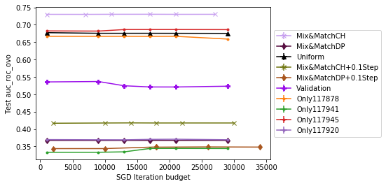
Figure 6: Test One vs One AUROC for predicting employee access in a new department

The experimental results are shown in Figure 6. Here, we observe that Mix&MatchCH has superior performance to all baseline algorithms. We also observe that, in this experiment, it seems that spending the entire budget searching over mixtures is more effective than spending only half of the SGD budget. Additionally, it seems that using the coordinate halving partitioning strategy produces better models than Mix&Match run with the Delaunay partitioning scheme.

References

- Allstate, (2014) Allstate (2014). Allstate Purchase Prediction Challenge. https://www.kaggle.com/c/allstate-purchase-prediction-challenge.
- Amazon, (2013) Amazon (2013). Amazon.com - Employee Access Challenge. https://www.kaggle.com/c/amazon-employee-access-challenge.
- Bahri, (2018) Bahri, D. (2018). wine ratings. https://www.kaggle.com/dbahri/wine-ratings.
- Bassily et al., (2016) Bassily, R., Nissim, K., Smith, A., Steinke, T., Stemmer, U., and Ullman, J. (2016). Algorithmic stability for adaptive data analysis. In Proceedings of the forty-eighth annual ACM symposium on Theory of Computing, pages 1046–1059. ACM.
- Bengio, (2011) Bengio, Y. (2011). Deep learning of representations for unsupervised and transfer learning. In Proceedings of the 2011 International Conference on Unsupervised and Transfer Learning workshop-Volume 27, pages 17–37. JMLR. org.
- Blum and Hardt, (2015) Blum, A. and Hardt, M. (2015). The ladder: A reliable leaderboard for machine learning competitions.
- Bottou et al., (2018) Bottou, L., Curtis, F. E., and Nocedal, J. (2018). Optimization methods for large-scale machine learning. Siam Review, 60(2):223–311.
- Bubeck, (2015) Bubeck, S. (2015). Convex optimization: Algorithms and complexity. Foundations and Trends® in Machine Learning, 8(3-4):231–357.
- Bubeck et al., (2011) Bubeck, S., Munos, R., Stoltz, G., and Szepesvári, C. (2011). X-armed bandits. Journal of Machine Learning Research, 12(May):1655–1695.
- Dai et al., (2009) Dai, W., Jin, O., Xue, G.-R., Yang, Q., and Yu, Y. (2009). Eigentransfer: a unified framework for transfer learning. In Proceedings of the 26th Annual International Conference on Machine Learning, pages 193–200. ACM.
- Defazio et al., (2014) Defazio, A., Bach, F., and Lacoste-Julien, S. (2014). Saga: A fast incremental gradient method with support for non-strongly convex composite objectives. In Advances in neural information processing systems, pages 1646–1654.
- Duchi et al., (2010) Duchi, J. C., Shalev-Shwartz, S., Singer, Y., and Tewari, A. (2010). Composite objective mirror descent. In COLT, pages 14–26.
- Gretton et al., (2009) Gretton, A., Smola, A., Huang, J., Schmittfull, M., Borgwardt, K., and Schölkopf, B. (2009). Covariate shift by kernel mean matching. Dataset shift in machine learning, 3(4):5.
- Grill et al., (2015) Grill, J.-B., Valko, M., and Munos, R. (2015). Black-box optimization of noisy functions with unknown smoothness. In Advances in Neural Information Processing Systems, pages 667–675.
- Hand and Till, (2001) Hand, D. J. and Till, R. J. (2001). A simple generalisation of the area under the roc curve for multiple class classification problems. Machine Learning, 45(2):171–186.
- Hardt, (2017) Hardt, M. (2017). Climbing a shaky ladder: Better adaptive risk estimation.
- Hardt et al., (2015) Hardt, M., Recht, B., and Singer, Y. (2015). Train faster, generalize better: Stability of stochastic gradient descent. arXiv preprint arXiv:1509.01240.
- Harvey et al., (2018) Harvey, N. J., Liaw, C., Plan, Y., and Randhawa, S. (2018). Tight analyses for non-smooth stochastic gradient descent. arXiv preprint arXiv:1812.05217.
- Heckman, (1977) Heckman, J. J. (1977). Sample selection bias as a specification error (with an application to the estimation of labor supply functions).
- Huang et al., (2007) Huang, J., Gretton, A., Borgwardt, K., Schölkopf, B., and Smola, A. J. (2007). Correcting sample selection bias by unlabeled data. In Advances in neural information processing systems, pages 601–608.
- Kearfott, (1978) Kearfott, B. (1978). A proof of convergence and an error bound for the method of bisection in . Mathematics of Computation, 32(144):1147–1153.
- Kornblith et al., (2018) Kornblith, S., Shlens, J., and Le, Q. V. (2018). Do better imagenet models transfer better? arXiv preprint arXiv:1805.08974.
- Mania et al., (2019) Mania, H., Miller, J., Schmidt, L., Hardt, M., and Recht, B. (2019). Model similarity mitigates test set overuse. arXiv preprint arXiv:1905.12580.
- Mohri et al., (2019) Mohri, M., Sivek, G., and Suresh, A. T. (2019). Agnostic federated learning. arXiv preprint arXiv:1902.00146.
- Munos, (2011) Munos, R. (2011). Optimistic optimization of a deterministic function without the knowledge of its smoothness. In Advances in neural information processing systems, pages 783–791.
- Nguyen et al., (2018) Nguyen, L. M., Nguyen, P. H., van Dijk, M., Richtárik, P., Scheinberg, K., and Takáč, M. (2018). SGD and Hogwild! Convergence Without the Bounded Gradients Assumption. arXiv e-prints, page arXiv:1802.03801.
- Oquab et al., (2014) Oquab, M., Bottou, L., Laptev, I., and Sivic, J. (2014). Learning and transferring mid-level image representations using convolutional neural networks. In Proceedings of the IEEE conference on computer vision and pattern recognition, pages 1717–1724.
- Pan and Yang, (2009) Pan, S. J. and Yang, Q. (2009). A survey on transfer learning. IEEE Transactions on knowledge and data engineering, 22(10):1345–1359.
- Raina et al., (2007) Raina, R., Battle, A., Lee, H., Packer, B., and Ng, A. Y. (2007). Self-taught learning: transfer learning from unlabeled data. In Proceedings of the 24th international conference on Machine learning, pages 759–766. ACM.
- Rakhlin et al., (2012) Rakhlin, A., Shamir, O., and Sridharan, K. (2012). Making gradient descent optimal for strongly convex stochastic optimization. In Proceedings of the 29th International Coference on International Conference on Machine Learning, pages 1571–1578. Omnipress.
- Roux et al., (2012) Roux, N. L., Schmidt, M., and Bach, F. R. (2012). A stochastic gradient method with an exponential convergence _rate for finite training sets. In Advances in neural information processing systems, pages 2663–2671.
- Sen et al., (2018) Sen, R., Kandasamy, K., and Shakkottai, S. (2018). Multi-fidelity black-box optimization with hierarchical partitions. In International Conference on Machine Learning, pages 4545–4554.
- Sen et al., (2019) Sen, R., Kandasamy, K., and Shakkottai, S. (2019). Noisy blackbox optimization using multi-fidelity queries: A tree search approach. In The 22nd International Conference on Artificial Intelligence and Statistics, pages 2096–2105.
- Shimodaira, (2000) Shimodaira, H. (2000). Improving predictive inference under covariate shift by weighting the log-likelihood function. Journal of statistical planning and inference, 90(2):227–244.
- Sugiyama et al., (2007) Sugiyama, M., Krauledat, M., and Müller, K.-R. (2007). Covariate shift adaptation by importance weighted cross validation. Journal of Machine Learning Research, 8(May):985–1005.
- Sugiyama et al., (2008) Sugiyama, M., Suzuki, T., Nakajima, S., Kashima, H., von Bünau, P., and Kawanabe, M. (2008). Direct importance estimation for covariate shift adaptation. Annals of the Institute of Statistical Mathematics, 60(4):699–746.
- Yosinski et al., (2014) Yosinski, J., Clune, J., Bengio, Y., and Lipson, H. (2014). How transferable are features in deep neural networks? In Advances in neural information processing systems, pages 3320–3328.
- Zadrozny, (2004) Zadrozny, B. (2004). Learning and evaluating classifiers under sample selection bias. In Proceedings of the twenty-first international conference on Machine learning, page 114. ACM.
- Zhao et al., (2019) Zhao, H., Combes, R. T. d., Zhang, K., and Gordon, G. J. (2019). On learning invariant representation for domain adaptation. arXiv preprint arXiv:1901.09453.
- Zhao et al., (2018) Zhao, S., Fard, M. M., Narasimhan, H., and Gupta, M. (2018). Metric-optimized example weights. arXiv preprint arXiv:1805.10582.