A Neural Network-Based On-device Learning Anomaly Detector for Edge Devices
Abstract
Semi-supervised anomaly detection is an approach to identify anomalies by learning the distribution of normal data. Backpropagation neural networks (i.e., BP-NNs) based approaches have recently drawn attention because of their good generalization capability. In a typical situation, BP-NN-based models are iteratively optimized in server machines with input data gathered from edge devices. However, (1) the iterative optimization often requires significant efforts to follow changes in the distribution of normal data (i.e., concept drift), and (2) data transfers between edge and server impose additional latency and energy consumption. To address these issues, we propose ONLAD and its IP core, named ONLAD Core. ONLAD is highly optimized to perform fast sequential learning to follow concept drift in less than one millisecond. ONLAD Core realizes on-device learning for edge devices at low power consumption, which realizes standalone execution where data transfers between edge and server are not required. Experiments show that ONLAD has favorable anomaly detection capability in an environment that simulates concept drift. Evaluations of ONLAD Core confirm that the training latency is 1.95x6.58x faster than the other software implementations. Also, the runtime power consumption of ONLAD Core implemented on PYNQ-Z1 board, a small FPGA/CPU SoC platform, is 5.0x25.4x lower than them.
Keywords On-device Learning Neural Networks Semi-supervised Anomaly Detection OS-ELM FPGA
1 Introduction
Anomaly detection is an approach to identify rare data instances (i.e., anomalies) that have different patterns or come from different distributions from that of the majority (i.e., the normal class) [1]. There are mainly three approaches in anomaly detection: (1) supervised anomaly detection, (2) semi-supervised anomaly detection, and (3) unsupervised anomaly detection.
(1) A typical strategy of supervised anomaly detection is to build a binary-classification model for the normal class vs. the anomaly class [1]. It requires labeled normal and anomaly data to train a model, however, anomaly instances are basically much rarer than normal ones, which imposes the class-imbalanced problem [2]. Several works have addressed this issue by undersampling the majority data or oversampling the minority data [3][4], or assigning more costs on misclassified data to make the classifier concentrate the minority classes [5].
(2) Semi-supervised anomaly detection, one of the main topics of this paper, assumes that all the training data belong to the normal class [1]. A typical strategy of semi-supervised anomaly detection is to learn the distribution of normal data and then to identify data samples distant from the distribution as anomalies. Semi-supervised approaches do not require anomalies to train a model, which makes them applicable to a wide range of real-world tasks. Various approaches have been proposed, such as nearest-neighbor based techniques [6][7], clustering approaches [8][9], and one-class classification approaches [10][11].
(3) Unsupervised anomaly detection does not require labeled training data [1], thus its constraint is the least restrictive. Many semi-supervised methods can be used in an unsupervised manner by using unlabeled data to train a model because most unlabeled data belong to the normal class. Sometimes, unsupervised anomaly detection and semi-supervised anomaly detection are not distinguished explicitly.
In this paper, we focus on semi-supervised anomaly detection. Recently, neural network-based approaches [12][13][14] have been drawing attention because in many cases they achieve relatively higher generalization performance than the traditional approaches for a wide range of real-world data such as images, natural languages, and audio data. Although there are some variants of neural networks, backpropagation neural networks (i.e., BP-NNs) are currently widely used.
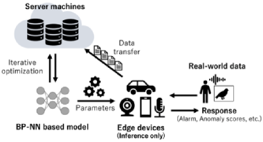
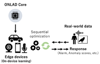
Figure 2 illustrates a typical application of BP-NN-based semi-supervised anomaly detection models. The system shown in the figure is designed for edge devices that implement their own models to detect anomalies of incoming real-world data. In this system, the edge devices are supposed to perform only inference computations (e.g., calculating anomaly scores), and training computations are offloaded to server machines. The models are iteratively trained in the server machines with a large amount of input data gathered from the edge devices. Once the training loop completes, parameters of the edge devices are updated with the optimized ones. However, there are two issues with this approach: (1) BP-NNs’ iterative optimization approach often takes a considerable computation time, which makes it difficult to follow time-series changes in the distribution of normal data (i.e., concept drift). (2) Data transfers to the server machines may impose several problems on the edge devices such as additional latency and energy consumption for communication.
(1) As mentioned before, learning the distribution of normal data is a key feature of semi-supervised anomaly detection approaches. However, the distribution may change over time. This phenomenon is referred to as concept drift. Concept drift is a serious problem when there are frequent changes in the surrounding environment of data [15] or behavioral state changes in data sources [16]. A semi-supervised anomaly detection model should learn new normal data to follow the changes, however, BP-NNs’ iterative optimization approach often introduces a considerable delay, which widens a gap between the latest true distribution of normal data and the one learned by the model [17]. This gap makes identifying anomalies more difficult gradually.
(2) Usually, edge devices that implement machine learning models are specialized only for prediction computations because the backpropagation method often requires a large amount of computational power. This is why training computations of BP-NNs are typically offloaded to server machines with high computational power. In this case, data transfers to the server machines are inevitable, which imposes additional energy consumption for communication and potential risk of data breaches on the edge devices.
One practical solution to these two issues is the on-device sequential learning approach illustrated in Figure 2. In this approach, incoming input data are sequentially learned on edge devices themselves. This approach allows the edge devices to sequentially follow changes in the distribution of normal data and makes possible standalone execution where no data transfers are required. However, it poses challenges in regard to how to construct such a sequential learning algorithm and how to implement it on edge devices with limited resources.
To deal with the underlying challenges, we propose an ON-device sequential Learning semi-supervised Anomaly Detector called ONLAD and its IP core, named ONLAD Core 111 This work is an extended version of our prior work [18]. . The algorithm of ONLAD is designed to perform fast sequential learning to follow concept drift in less than one millisecond. ONLAD Core realizes on-device learning for resource-limited edge devices at low power consumption.
In this paper, we make the following contributions:
-
1.
ONLAD leverages OS-ELM [19], a lightweight neural network that can perform fast sequential learning, as a core component. In Section 3.1, we theoretically analyze the training algorithm of OS-ELM and demonstrate that the computational cost significantly reduces without degrading the training results when the batch size equals 1.
-
2.
In Section 3.2, we propose a computationally lightweight forgetting mechanism for OS-ELM based on FP-ELM, a state-of-the-art OS-ELM variant with a dynamic forgetting mechanism. Since a key feature of semi-supervised anomaly detection is to learn the distribution of normal data, OS-ELM should be able to forget past learned normal data when the distribution changes. The proposed method provides such a function for OS-ELM with a tiny additional computational cost.
-
3.
In Section 3.3, we propose ONLAD, a new sequential learning semi-supervised anomaly detector that combines OS-ELM and an autoencoder [20], a neural network-based dimensionality reduction model. This combination, together with the other proposed techniques to reduce the computational cost, realizes fast sequential learning semi-supervised anomaly detection. Experiments using several public datasets in Section 5 show that ONLAD has comparable generalization capability to that of BP-NN based models in the context of anomaly detection. They also confirm that ONLAD outperforms BP-NN based models in terms of anomaly detection capability especially in an environment that simulates concept drift.
-
4.
In Section 4, we describe the design and implementation of ONLAD Core. Evaluations of ONLAD Core in Section 6 show that ONLAD Core can perform training and prediction computations approximately in less than one millisecond. In comparison with software counterparts, the training latency of ONLAD Core is faster by 1.95x6.58x, while the prediction latency is faster by 2.29x4.73x on average. They also confirm that the proposed forgetting mechanism is faster than the baseline algorithm, FP-ELM, by 3.21x on average. In addition, our evaluations show that ONLAD Core can be implemented on PYNQ-Z1 board, a small FPGA/CPU SoC platform, in practical model sizes. It is also demonstrated that the runtime power consumption of PYNQ-Z1 board that implements ONLAD Core is 5.0x25.4x lower than the other software counterparts when training computations are continuously executed.
The rest of this paper is organized as follows: Section 2 provides a brief review of the basic technologies behind ONLAD. We propose ONLAD in Section 3. Section 4 describes the design and implementation of ONLAD Core. ONLAD is evaluated in terms of anomaly detection capability in Section 5. ONLAD Core is also evaluated in terms of latency, FPGA resource utilization, and power consumption in Section 6. Related works are described in Section 7. Section 8 concludes this paper.
2 Preliminaries
This section provides a brief introduction of the base technologies behind ONLAD: (1) ELM (Extreme Learning Machine), (2) OS-ELM (Online Sequential Extreme Learning Machine), and (3) autoencoders.
2.1 ELM
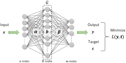
ELM [21] illustrated in Figure 3 is a kind of single hidden layer feedforward network (i.e., SLFN) that consists of an input layer, a hidden layer, and an output layer. Suppose an -dimensional input chunk of batch size is given; an -dimensional output chunk is computed as follows.
| (1) |
where denotes an input weight connecting the input layer and the hidden layer, and an output weight connecting the hidden layer and the output layer. denotes a bias vector of the hidden layer, and an activation function applied to the hidden layer output.
If an SLFN can approximate an -dimensional target chunk with zero error, it implies that there exists which satisfies the following equation.
| (2) |
Let be the hidden layer output ; then the optimal output weight is computed as follows.
| (3) |
where is the pseudo inverse of . can be calculated with matrix decomposition algorithms such as SVD (Singular Value Decomposition) [22]. In particular, if or is non-singular, can be calculated in an efficient way with or .
The whole training process is completed simply by replacing with . and do not change once they have been initialized with random values; the conversion from to is random projection.
ELM does not use iterative optimization that BP-NNs use, but rather one-shot optimization, which makes the whole training process faster. ELM can compute the optimal output weight faster than BP-NNs [21]. It is categorized as a batch learning algorithm, wherein all the training data are assumed to be available in advance. In other words, ELM must be retrained with the whole dataset, including the past training data, in order to learn new instances.
2.2 OS-ELM
OS-ELM [19] is an ELM variant that can perform sequential learning instead of batch learning. Suppose the th training chunk of batch size is given; we need to find that minimizes the following error.
| (4) |
where is defined as . The optimal output weight is sequentially computed as follows.
| (5) |
and are computed as follows.
| (6) |
The number of initial training samples should be greater than that of hidden nodes to make nonsingular.
2.3 Autoencoders

An autoencoder [20] illustrated in Figure 4 is a neural network-based unsupervised learning model for finding a well-characterized dimensionality reduced form of an input chunk (). Generally, the output of an intermediate layer is regarded as . ELM and OS-ELM have only one intermediate layer; therefore, the hidden layer output is regarded as . Basically, the number of hidden nodes is constrained to be less than that of input nodes . Such autoencoders are specially referred to as undercomplete autoencoders. However, sometimes they take the opposite setting (i.e., ) where they are referred to as overcomplete autoencoders. Although overcomplete autoencoders cannot perform dimensionality reduction, they can obtain well-characterized representations for classification problems by applying regularization conditions or noise [23] to their loss functions.
In the training process, input data are also used as targets (i.e., ); therefore, an autoencoder is trained to correctly reconstruct input data as output data. It is empirically known that tends to become well-characterized when the error between input data and reconstructed output data converges [20]. Labeled data are not required during the whole training process; this is why an autoencoder is categorized as an unsupervised learning model.
Autoencoders have been attracting attention in the field of semi-supervised anomaly detection [13][24], too. In this context, an autoencoder is trained only with normal data; therefore, its output tends to have a relatively large reconstruction error in the case of an anomaly. Thus, anomalies can be detected by setting a threshold for the errors. This approach is categorized as a semi-supervised anomaly detection method since only normal data are used as training data.
PCA (Principal Component Analysis), another non-statistical dimensionality reduction algorithm, is often compared with autoencoders. Sakurada et al. showed that autoencoder-based models can detect subtle anomalies that PCA fails to pick up [13]. Moreover, autoencoders can perform nonlinear transformations without costly computations that kernel PCA [25] requires.
3 ONLAD
As mentioned in the introduction, ONLAD leverages OS-ELM as its core component. In this section, we provide a theoretical analysis of OS-ELM and demonstrate that the computational cost of the training algorithm significantly reduces when batch size = 1 without any deterioration of the training results. Then, we propose a computationally lightweight forgetting mechanism to deal with concept drift. Finally, we formulate the algorithm of ONLAD.
3.1 Analysis of OS-ELM
The training algorithm of OS-ELM (i.e., Equation 5) mainly consists of (1) matrix products and (2) matrix inversions. Suppose the computational iterations of a matrix product are and those of a matrix inversion are ; the total computational iterations of these two operations in Equation 5 are calculated as follows.
where denotes the total computational iterations of the matrix products, while denotes those of the matrix inversions. , , and are the numbers of input, hidden, and output nodes of OS-ELM, respectively. denotes the batch size. For instance, the computational iterations of are calculated by dividing the computing process into two steps: (1) and (2) . In this case, these computational iterations are calculated as and , respectively.
Let be the total computational iterations of matrix products and matrix inversions in Equation 5 when batch size = . Accordingly, the following equations can be derived.
Finally, is obtained. This inequality shows that the training algorithm becomes computationally more efficient when batch size = 1, rather than when batch size = . Please note that this insight does not always make sense especially for software implementations because this computational model does not take into account the software-specific overheads such as memory allocation and function calls. However, bare-metal implementations, including ONLAD Core, receive benefits from this insight since they are free from such overheads. Moreover, when = 1, the computational cost of the matrix inversion in Equation 5 is significantly reduced, as the size of the target matrix is . In this case, the following training algorithm is derived from Equation 5.
| (7) |
where denotes the special case of when = 1. Thanks to the above trick, OS-ELM can perform training without any costly matrix inversions, which helps to reduce not only the computational cost but also the hardware resources needed for ONLAD Core. It also makes it easier to parallelize the training algorithm, because there are no matrix inversions with a low degree of parallelism in Equation 7. Furthermore, the training results of OS-ELM are not affected even when batch size = 1, because OS-ELM gives the same output weight when training is performed times with batch size = or times with batch size = 1. This is a notable difference from BP-NNs; their training results get better or worse depending on the batch size. On the basis of the above discussion, the batch size of OS-ELM used in ONLAD is always set to 1.
3.2 Lightweight Forgetting Mechanism for OS-ELM
In certain real environments, the distribution of normal data may change as time goes by. In this case, ONLAD should have a function to adaptively forget past learned normal data with a tiny additional computational cost. To deal with this challenge, we propose a computationally lightweight forgetting mechanism based on FP-ELM (Forgetting Parameters Extreme Learning Machine) [26], a state-of-the-art OS-ELM variant with a dynamic forgetting mechanism.
3.2.1 Review of FP-ELM
This section provides a brief review of FP-ELM. The training algorithm of FP-ELM is formulated as follows.
| (8) |
Especially, and are computed as follows.
| (9) |
where is the L2 regularization parameter for . limits so that it does not become too large to prevent overfitting. is the forgetting factor that controls the weight (i.e., the significance) of each past training chunk. Suppose the latest training step is ; then , the weight of the th training chunk, is gradually decreased from one step to the next, as shown below.
| (12) |
Please note that is a variable parameter that can be adaptively updated according to the information in the arriving input data or output error values.
3.2.2 Proposed Forgetting Mechanism
FP-ELM can control the weights of past training chunks. However, it cannot remove the matrix inversion in Equation 8 even when the batch equals 1, because the size of the target matrix is , where denotes the number of hidden nodes. To address this issue, we modify FP-ELM so that it can remove the matrix inversion when batch size = 1.
First, the following equations are derived by disabling the L2 regularization trick (i.e., let = 0) in Equation 8.
| (13) |
Next, the update formula of is derived with the Woodbury formula [27] 222.
| (14) |
Finally, the training algorithm is obtained by defining .
| (15) |
and are computed with the same algorithm as Equation 6. The proposed forgetting mechanism eliminates the matrix inversion in Equation 15 when batch size = 1 because the size of the target matrix is , where denotes the batch size. Equation 15 becomes equal to the original training algorithm of OS-ELM when is replaced with . Thus, the proposed method provides a forgetting function with a tiny additional computational cost to the original training algorithm of OS-ELM. However, it may suffer from overfitting, since the L2 regularization trick is disabled. The trade-off is quantitatively evaluated in Section 5.
3.3 Algorithm
ONLAD leverages OS-ELM of batch size = 1 in conjunction with the proposed forgetting mechanism. The following equations are derived by combining Equations 7 and 15.
| (16) |
ONLAD is built on an OS-ELM-based autoencoder to construct a semi-supervised anomaly detector; holds in Equation 16. The training algorithm of ONLAD is as follows.
| (17) |
and are computed as follows (there are no changes from Equation 6).
| (18) |
As indicated in Equation 17, ONLAD performs training and forgetting operations at the same time.
The prediction algorithm is formulated as follows.
| (19) |
where denotes a loss function, and is an anomaly score of .
3.4 Stability of OS-ELM Training
OS-ELM has a training stability issue: if in Equation 5 is close to a singular matrix, the training becomes unstable regardless of the batch size [19]. In the context of ONLAD, the problem occurs when in Equation 17 is close to 0. Thus, ONLAD should stop the training when , where denotes a small positive value.
3.5 Example of ONLAD in Practical Use
The following is an example of ONLAD (shown in Algorithm 1) intended for practical use. First, and are initialized with random values; then and are computed with Equation 18. Please note that the number of initial training samples should be larger than that of hidden nodes to make nonsingular. At the th training step in the following loop, the inequality is evaluated, then the rest of the lines are skipped if it is true. If it is false, then an anomaly score of is computed with Equation 19. is judged to be an anomaly if the score is greater than a user-defined threshold ; otherwise ONLAD judges to be a normal sample. Finally, sequential learning is performed with Equation 17.
| Board Specifications | ||||
|---|---|---|---|---|
| Linux Image | PYNQ v2.4 (Ubuntu v18.04) | |||
| SoC Chip |
|
|||
| DRAM | DDR3 512MB | |||
| FPGA Specifications | ||||
| BRAM | 280 blocks | |||
| DSP | 220 slices | |||
| FF | 106,400 instances | |||
| LUT | 53,200 instances | |||
4 ONLAD Core
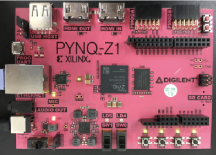
This section describes the design and implementation of ONLAD Core, an IP core of ONLAD. To demonstrate that ONLAD Core can be implemented on edge devices with limited resources, we use PYNQ-Z1 board, a low-cost SoC platform where an FPGA is integrated. Figure 5 displays the board, and its specifications are shown in Table 5. We develop ONLAD Core with Vivado HLS v2018.3 and implement it on PYNQ-Z1 board using Vivado v2018.3. The clock frequency of ONLAD Core is set to 100.0 MHz.
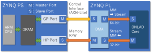
4.1 Overview of Board-level Implementation
First, we provide a brief overview of our board-level implementation. Figure 7 shows the block diagram. The PS (Processing System) part is mainly responsible for preprocessing of input data and triggering a DMA (Direct Memory Access) controller. The DMA controller converts preprocessed input data in DRAM to AXI4-Stream format packets and transfers them to ONLAD Core. It also converts output packets of ONLAD Core back to AXI4-Memory-Mapped format data, and transfers them to DRAM. On the other hand, the PL (Programmable Logic) part implements ONLAD Core. ONLAD Core performs training or prediction computations according to the information in the header of input packets (the details are to be described later).
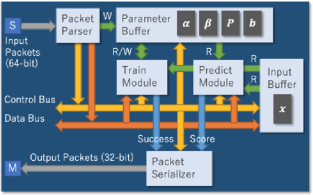
4.2 Details of ONLAD Core
Figure 7 illustrates the block diagram of ONLAD Core, with its four important sub-modules: (1) Parameter Buffer, (2) Input Buffer, (3) Train Module, and (4) Predict Module. The rest of this section explains these sub-modules one by one.
4.2.1 Parameter Buffer
Parameter Buffer manages the parameters of ONLAD Core (i.e., , , , and ). All the parameters are implemented with BRAMs; hence, more BRAM instances are consumed as the sizes of the parameters increase. Specifically, the total number of matrix elements of Parameter Buffer (denoted as ) is calculated as follows.
| (20) |
Please note that is applied in Equation 20, since ONLAD is an autoencoder. Equation 20 shows that the utilization of the BRAM instances of this module is proportional to the square of the number of hidden nodes and is also proportional to the number of input nodes .
4.2.2 Input Buffer
Input Buffer stores a single input vector preprocessed in the PS part and, like Parameter Buffer, is implemented with BRAMs. The total number of matrix elements of Input Buffer (denoted as ) is calculated as follows.
| (21) |
Equation 21 shows that the utilization of the BRAM instances of this module is proportional to the number of input nodes . This module is shared with Train Module and Predict Module so that they can read the input vector.
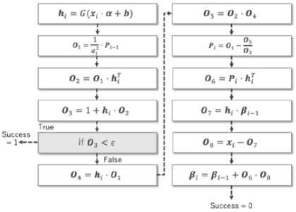
4.2.3 Train Module
Train Module executes the training algorithm (i.e., Equation 17) in order to update the parameters in Parameter Buffer. Figure 9 shows the processing flow. Each processing block is sequentially executed. According to the discussion in Section 3.4, Train Module is designed to interrupt the computation when holds. In our implementation, is set to . The output signal of indicates whether the inequality is satisfied or not (1/0 means satisfied/not satisfied). All the matrix operations, including matrix products, matrix adds, matrix subs, and element-wise multiplies are implemented with arithmetic units of 32-bit fixed-point precision using DSPs. To save hardware resources, these matrix operations are designed to use a specific number of arithmetic units regardless of the number of input and hidden nodes. The matrices shown in the processing flow (i.e., and ) are implemented with BRAMs.
The total number of matrix elements of Train Module (denoted as ) is calculated as follows.
| (22) |
Equation 22 shows that the utilization of the BRAM instances of this module is proportional to the square of the number of hidden nodes and is also proportional to the number of input nodes .
below denotes the total computational iterations needed to finish the processing flow, calculated in the manner described in Section 3.1.
| (23) |
The computational cost is proportional to the square of the number of hidden nodes , and is also proportional to the number of input nodes .
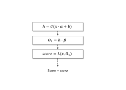
4.2.4 Predict Module
Predict Module executes the prediction algorithm (i.e., Equation 19) to output anomaly scores. Figure 9 shows the processing flow. Predict Module follows the design methodology of Train Module.
The total number of matrix elements of Predict Module (denoted as ) is calculated as follows.
| (24) |
Equation 24 shows that the utilization of the BRAM instances of this module is proportional to the numbers of hidden nodes and input nodes .
below denotes the total computational iterations to finish the processing flow.
| (25) |
The computational cost is proportional to the numbers of hidden nodes and input nodes .
4.2.5 Implementation of Matrix Operations
In ONLAD Core, matrix operations, such as matrix product, matrix add, matrix sub, and element-wise multiply, are implemented as a dedicated circuit. These matrix operations are designed with C-level language and synthesized with Vivado HLS. Loop unrolling and loop pipelining directives are used in the innermost loops of these operations for parallelization. In this design, unrolling factor is set to 2, so that they are parallelized with two arithmetic units.
4.3 Instructions of ONLAD Core
ONLAD Core is designed to execute the following instructions: (1) update_params, (2) update_input, (3) update_ff, (4) do_training, and (5) do_prediction. The packet format of each instruction is detailed in Figure 10. An input packet is of 64 bits long. The first 3-bit field (i.e., Mode Field) specifies an instruction to be executed on ONLAD Core. The following 61-bit field (i.e., Data Field) is reserved for several uses according to the instruction. An output packet is of 32 bits long and embeds an output result of Train Module or Predict Module.
In the rest of this section, we describe how the sub-modules of ONLAD Core work according to each instruction.
4.3.1 update_params
This instruction updates Parameter Buffer. The packet format is shown in the first row of Figure 10. The target parameter is specified in Mode Field of an input packet. in Data Field embeds an index of the target parameter, and an update value. The target parameter is updated as below.
| (26) |
Please note that all the parameters are managed as row-major flattened 1-D arrays in Parameter Buffer.
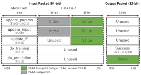
4.3.2 update_input
This instruction updates Input Buffer. The packet format (the second row of Figure 10) is almost the same as update_params instruction except for Mode Field.
| (27) |
Input Buffer is updated with the above formula. Please note that input packets are required to create an -dimensional input vector.
4.3.3 update_ff
This instruction updates the forgetting factor managed in Train Module. The packet format of this instruction is shown in the third row of Figure 10. in Data Field embeds an update value. is updated as follows.
| (28) |
4.3.4 do_training
This instruction executes training computations with Train Module. Train Module first reads the latest parameters (i.e., and ) from Parameter Buffer, and an input vector from Input Buffer. Then, it executes the training algorithm and updates Parameter Buffer with the new parameters (i.e., and ).
4.3.5 do_prediction
This instruction executes prediction computations with Predict Module. Predict Module reads the latest output weight if it is updated, and an input vector in the same way as Train Module. Predict Module then executes the prediction algorithm and outputs an anomaly score of the input vector.
The packet format is shown in the last row of Figure 10. An input packet of this instruction is also just a trigger for prediction. An output packet of this instruction embeds an output anomaly score (denoted as ) computed by ONLAD Core.
5 Evaluation of ONLAD
In this section, the anomaly detection capability of ONLAD is evaluated in comparison with other models. A common server machine (OS: Ubuntu 18.04, CPU: Intel Core i7 6700 3.4GHz, GPU: Nvidia GTX 1070 8GB, DRAM: DDR4 16GB, and Storage: SSD 512GB) is used as the experimental machine in this section and Section 6.
| ONLAD | FPELM-AE | |
| {Sigmoid [31], Identity33footnotemark: 3} | {Sigmoid, Identity} | |
| Uniform [0,1] | Uniform [0,1] | |
| MSE444 | MSE | |
| {0.95, 0.96, …, 1.00} | {0.95, 0.96, …, 1.00} | |
| {8, 16, 32, …, 256} | {8, 16, 32, …, 256} | |
| 0.02555 | ||
| NN-AE | DNN-AE | |
| {Sigmoid, Relu [32]} | {Sigmoid, Relu} | |
| Sigmoid | Sigmoid | |
| MSE | MSE | |
| Adam [33] | Adam | |
| {8, 16, 32} | {8, 16, 32} | |
| {5, 10, 15, 20} | {5, 10, 15, 20} | |
| {8, 16, 32, …, 256} | {8, 16, 32, …, 256} | |
| {8, 16, 32, …, 256} | ||
| {8, 16, 32, …, 256} |
5.1 Experimental Setup
ONLAD is compared with the following models: (1) FPELM-AE, (2) NN-AE, and (3) DNN-AE. FPELM-AE is an FP-ELM-based autoencoder. This model is used to quantitatively evaluate the effect of disabling the L2 regularization trick in ONLAD. NN-AE is a 3-layer BP-NN-based autoencoder, and DNN-AE is a BP-NN-based deep autoencoder consisting of five layers. These models are used to compare OS-ELM-based autoencoders (i.e., FPELM-AE and ONLAD) with BP-NN-based ones. All the models, including ONLAD, were implemented with TensorFlow v1.13.1 [34].
For a comprehensive evaluation, two testbeds: (1) Offline Testbed and (2) Online Testbed are conducted. Offline Testbed simulates an environment where all training and test data are available in advance and no concept drift occurs. This is a standard experimental setup to evaluate semi-supervised anomaly detection models. The purpose of Offline Testbed is to measure the generalization capability of ONLAD in the context of anomaly detection. This testbed is not used to evaluate the proposed forgetting mechanism (i.e., is always fixed to 1), since no concept drift occurs in this testbed. On the other hand, Online Testbed simulates an environment where at first only a small part of a dataset is given and the rest arrives as time goes by. Online Testbed assumes that concept drift occurs. The purpose of this testbed is to evaluate the robustness of the proposed forgetting mechanism against concept drift in comparison with the other models.
Several public classification datasets listed in Table 2 are used to construct Offline Testbed and Online Testbed. All data samples are normalized within [0,1] by using min-max normalization. Hyperparameters of each model are explored within the ranges detailed in Table 3666 : an activation function applied to all the hidden layers. : an activation function applied to the output layer. : a probability density function used for random initialization of ONLAD and FPELM-AE. : the number of nodes of the th hidden layer. : a loss function. : the forgetting factor of ONLAD and FPELM-AE. : the L2 regularization parameter of FPELM-AE. : an optimization algorithm. : batch size. : the number of training epochs. . 66footnotetext: This value was used for the experiments in the original paper of FP-ELM (i.e., [26]).
5.2 Experimental Method
This section describes the experimental methods of Offline Testbed and Online Testbed, respectively.
Algorithm 2 shows the experimental method of Offline Testbed. In this testbed, a dataset is divided into training data (80%) and test data (20%), respectively. Suppose we have a dataset that consists of classes in total; training data of class are used as normal data for training (denoted as ) and test data of class are as normal data for testing (denoted as ). Test data of class are used as anomaly data (denoted as ). The number of samples in is limited up to 10% of that of to simulate a practical situation; anomaly data are much rarer than normal data in most cases. A model is trained with (NN-AE and DNN-AE are trained with batch size = for epochs). Once the training procedure is finished, the model is evaluated with a test set that mixes and , then an AUC (Area Under Curve) score is calculated. AUC is one of the most widely used metrics for evaluating the accuracy of anomaly detection models independently of particular anomaly score thresholds. The above process is repeated until , then all the AUC scores are averaged. The output score is recorded as a result of a single trial; the final AUC scores reported in Table 4 are averages over 50 trials. 10-fold cross-validation is conducted for hyperparameter tuning.
Algorithm 3 shows the experimental method of Online Testbed. In this testbed, a dataset is divided into initial data (10%), test data (45%), and validation data (45%). represents for data samples that exit in the begining. and represent for data samples that sequentially arrive as time goes by. is used to measure the final AUC scores, while is only for hyperparameter tuning. Both are further divided into normal data (90%) and anomaly data (10%). In the first step, a list (denoted as ) consisting of integers 0 is constructed and randomly shuffled. The output indicates the normal class of each concept; e.g., supposing that , the normal class of the 0/1/2th concept is 2/0/1. The th concept mixes normal data of class and anomaly data of class . The number of anomaly samples per one concept is limited to 10% of that of normal samples. A model is trained with initial data of the first normal class (NN-AE and DNN-AE are trained with batch size = for epochs). Then, the model computes an anomaly score for each data sample continuously given from . Every time an anomaly score is computed, the model is trained with the data sample (all the models, including NN-AE and DNN-AE, are trained with batch size = 1 to sequentially follow the transition of the normal class). After all the data samples are fed to the model, an AUC score is calculated with the anomaly scores. This AUC score is recorded as a result of a single trial; the final AUC scores reported in Table 5 are averages over 50 trials. Hyperparameter tuning is conducted with the same algorithm for 10 trials by replacing with in Algorithm 3.
| Dataset | ONLAD | FPELM-AE | NN-AE | DNN-AE |
|---|---|---|---|---|
| Fashion MNIST | 0.905 | 0.905 | 0.925 | 0.913 |
| MNIST | 0.944 | 0.945 | 0.958 | 0.961 |
| Smartphone HAR | 0.929 | 0.928 | 0.922 | 0.910 |
| Drive Diagnosis | 0.939 | 0.943 | 0.952 | 0.961 |
| Letter Recognition | 0.952 | 0.950 | 0.978 | 0.985 |
| Dataset | ONLAD-NF | ONLAD | FPELM-AE | NN-AE | DNN-AE |
|---|---|---|---|---|---|
| Fashion MNIST | 0.575 | 0.869 | 0.866 | 0.685 | 0.697 |
| MNIST | 0.591 | 0.899 | 0.898 | 0.787 | 0.755 |
| Smartphone HAR | 0.558 | 0.781 | 0.788 | 0.785 | 0.799 |
| Drive Diagnosis | 0.552 | 0.786 | 0.849 | 0.744 | 0.853 |
| Letter Recognition | 0.548 | 0.882 | 0.879 | 0.737 | 0.788 |
5.3 Experimental Results
The experimental results for Offline Testbed are shown in Table 4. The hyperparameter settings are also listed in Table 6. Here, NN-AE and DNN-AE achieve slightly higher AUC scores than those of ONLAD by approximately 0.010.03 point on almost all the datasets. This result implies that BP-NN-based autoencoders have slightly higher generalization capability than that of OS-ELM-based ones in the context of anomaly detection. However, NN-AE and DNN-AE have to be iteratively trained for some epochs in order to achieve their best performance (here, they were trained for 520 epochs). In contrast, ONLAD always finds the optimal output weight in only one epoch. Also, ONLAD achieves its best AUC scores with an equal or smaller size compared with NN-AE and DNN-AE for all the datasets, which helps to reduce the computational cost and save on hardware resources required to implement ONLAD Core. In addition, the differences between the AUC scores of ONLAD and FPELM-AE are within 0.0010.004 point; ONLAD keeps favorable generalization performance even when the L2 regularization trick is disabled. In summary, ONLAD has comparable generalization capability to that of the BP-NN-based models in much smaller training epochs with an equal or smaller model size.
The experimental results for Online Testbed are shown in Table 5. The hyperparameter settings are also listed in Table 7. Here, another model, named ONLAD-NF (ONLAD-No-Forgetting-mechanism) is introduced in order to examine the effectiveness of the proposed forgetting mechanism. ONLAD-NF is the special case of ONLAD, where the forgetting mechanism is disabled by setting to 1. The hyperparameter settings of ONLAD-NF are the same as those of ONLAD, except for . As shown in the table, ONLAD-NF suffers from significantly lower AUC scores than ONLAD. The reason is quite obvious; ONLAD-NF does not have any functions to forget past learned data, therefore it gradually becomes more difficult to detect anomalies every time concept drift happens. NN-AE and DNN-AE, on the other hand, achieve much higher AUC scores than ONLAD-NF because BP-NNs have the catastrophic forgetting nature [35], which works as a kind of forgetting mechanism. However, BP-NNs do not have any numerical parameters to analytically control the progress of forgetting, unlike ONLAD. For this reason, ONLAD stably achieves more favorable AUC scores. Additionally, ONLAD and FPELM-AE have similar AUC scores on most of the datasets, as with the results on Offline Testbed. This result shows that the proposed forgetting mechanism is not significantly affected by the L2 regularization trick on these datasets. In summary, ONLAD achieves much higher AUC scores than those of NN-AE and DNN-AE by approximately 0.100.18 point on three datasets out of the five ones. It also achieves comparable AUC scores to those of the BP-NN-based models on the other two datasets.
| Dataset |
|
|
||||
|---|---|---|---|---|---|---|
| Fashion MNIST | Identity, Uniform, 64, MSE, 1.00 | Identity, Uniform, 64, MSE, 1,00, 0.02 | ||||
| MNIST | Identity, Uniform, 64, MSE, 1.00 | Identity, Uniform, 64, MSE, 1.00, 0.02 | ||||
| Smartphone HAR | Identity, Uniform, 128, MSE, 1.00 | Identity, Uniform, 128, MSE, 1.00, 0.02 | ||||
| Drive Diagnosis | Sigmoid, Uniform, 16, MSE, 1.00 | Sigmoid, Uniform, 16, MSE, 1.00, 0.02 | ||||
| Letter Recognition | Sigmoid, Uniform, 8, MSE, 1.00 | Sigmoid, Uniform, 8, MSE, 1.00, 0.02 | ||||
| Dataset |
|
|
||||
| Fashion MNIST | Relu, Sigmoid, 64, MSE, Adam, 32, 5 | Relu, Sigmoid, 64, 32, 64, MSE, Adam, 8, 10 | ||||
| MNIST | Relu, Sigmoid, 64, MSE, Adam, 32, 5 | Relu, Sigmoid, 64, 32, 64, MSE, Adam, 8, 10 | ||||
| Smartphone HAR | Relu, Sigmoid, 256, MSE, Adam, 8, 20 | Relu, Sigmoid, 128, 256, 128, MSE, Adam, 8, 20 | ||||
| Drive Diagnosis | Relu, Sigmoid, 256, MSE, Adam, 8, 10 | Relu, Sigmoid, 128, 256, 128, MSE, Adam, 8, 20 | ||||
| Letter Recognition | Relu, Sigmoid, 256, MSE, Adam, 8, 20 | Relu, Sigmoid, 128, 256, 128, MSE, Adam, 8, 20 |
| Dataset |
|
|
||||
|---|---|---|---|---|---|---|
| Fashion MNIST | Sigmoid, Uniform, 64, MSE, 0.99 | Sigmoid, Uniform, 64, MSE, 0.99, 0.02 | ||||
| MNIST | Sigmoid, Uniform, 64, MSE, 0.99 | Sigmoid, Uniform, 64, MSE, 0.99, 0.02 | ||||
| Smartphone HAR | Identity, Uniform, 16, MSE, 0.97 | Sigmoid, Uniform, 16, MSE, 0.97, 0.02 | ||||
| Drive Diagnosis | Sigmoid, Uniform, 16, MSE, 0.99 | Sigmoid, Uniform, 16, MSE, 0.97, 0.02 | ||||
| Letter Recognition | Identity, Uniform, 8, MSE, 0.95 | Identity, Uniform, 8, MSE, 0.95, 0.02 | ||||
| Dataset |
|
|
||||
| Fashion MNIST | Relu, Sigmoid, 64, MSE, Adam, 32, 5 | Relu, Sigmoid, 64, 32, 64, MSE, Adam, 8, 10 | ||||
| MNIST | Relu, Sigmoid, 64, MSE, Adam, 32, 5 | Relu, Sigmoid, 64, 32, 64, MSE, Adam, 8, 10 | ||||
| Smartphone HAR | Sigmoid, Sigmoid, 32, MSE, Adam, 8, 20 | Sigmoid, Sigmoid, 32, 2, 32, MSE, Adam, 8, 20 | ||||
| Drive Diagnosis | Sigmoid, Sigmoid, 16, MSE, Adam, 8, 10 | Sigmoid, Sigmoid, 16, 8, 16, MSE, Adam, 8, 20 | ||||
| Letter Recognition | Relu, Sigmoid, 16, MSE, Adam, 8, 20 | Relu, Sigmoid, 16, 8, 16, MSE, Adam, 8, 20 |
6 Evaluations of Performance and Cost
In this section, ONLAD Core is evaluated in terms of latency, FPGA resource utilization, and power consumption in comparison with software implementations.
6.1 Experimental Setup
ONLAD Core is evaluated in comparison with the following software implementations: (1) NN-AE-CPU, (2) DNN-AE-CPU, (3) NN-AE-GPU, (4) DNN-AE-GPU, (5) FPELM-AE-CPU, and (6) FPELM-AE-GPU. {*}-CPU is executed only with a CPU, while {*}-GPU is executed with a GPU in cooperation with a CPU. All of these implementations are developed with Tensorflow v1.13.1. Here, Tensorflow v1.13.1 is built with AVX2 (Advanced Vector eXtensions 2) instructions and -O3 option to accelerate CPU computations. It is also built with CUDA [36] v10.0 to enable GPGPU execution.
The hyperparameter settings of the above implementations are detailed in Table 8. , , and have been omitted from the table because these parameters are unrelated to any of the evaluation metrics (i.e., latency, FPGA resource utilization, and power consumption). The batch size (i.e., ) of NN-AE-{*} and DNN-AE-{*} is fixed to 1, as with ONLAD Core and FPELM-AE-{*} in order to conduct fair comparisons of latency and power consumption.
6.2 Latency
6.2.1 Training/Prediction Latency
Here, we refer to “training latency” as the elapsed time from when a model receives an input sample until the training algorithm is computed. “Prediction latency” is the elapsed time from when a model receives an input data sample until an anomaly score is calculated.
Figures 11 and 12 show the training and prediction latency times of each implementation versus the numbers of input and hidden nodes (all the reported times are averages over 50,000 trials). To measure practical latency times, the exploration range of the number of input nodes is set to {128, 256, 512, 1,024}, while that of the number of hidden nodes is set to {16, 32, 64} on the basis of the hyperparameter settings of ONLAD in Section 5.
|
|
|
|
||||||||
|---|---|---|---|---|---|---|---|---|---|---|---|
| Identity, , MSE | Relu, Sigmoid, , MSE, Adam, 1 | Relu, Sigmoid, , , , MSE, Adam, 1 | Identity, , MSE |
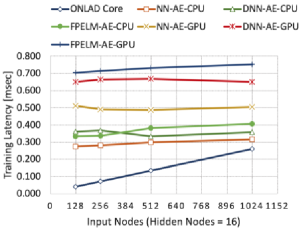
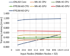
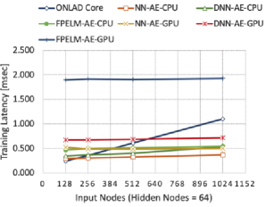
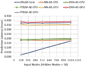
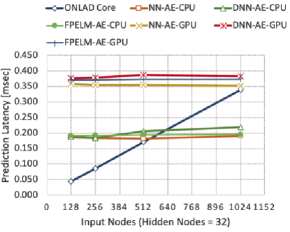
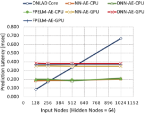
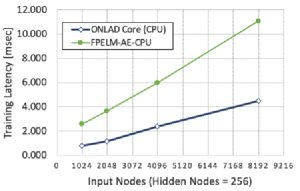

As shown in the figures, the latency times of the software implementations remain almost constant as the number of input nodes increases. This outcome shows that most of their execution times are occupied with software overheads to invoke training and prediction tasks. The GPU-based implementations especially suffer from high latency times because of the communication cost between a GPU and a CPU in addition to the software overheads. In contrast, ONLAD Core is free from these overheads. Consequently, ONLAD Core achieves 1.95x, 2.45x, 2.56x, 3.38x, 4.51x, and 6.58x speedups on average over NN-AE-CPU, DNN-AE-CPU, FPELM-AE-CPU, NN-AE-GPU, DNN-AE-GPU, and FPELM-AE-GPU in terms of training latency, and 2.29x, 2.37x, 2.36x, 4.38x, 4.73x, and 4.57x speedups on average over them in terms of prediction latency. ONLAD Core can perform fast sequential learning and prediction to follow concept drift approximately in less than one millisecond.
However, please note that ONLAD Core may become slower than the others when there are many input nodes since the computational cost of Train/Predict Module is proportional to the number of input nodes, as shown in Equations 23 and 25. Hence, ONLAD Core has difficulty achieving speedups beyond 1.0x over the software implementations when there are thousands of input nodes.
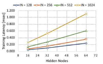
Moreover, the computational cost of Train Module is proportional to the square of the number of hidden nodes, too. However, contrary to expectations, Figure 14 shows that the latency times are almost proportional to the number of hidden nodes. This is because holds as long as in Equation 23. In other words, the computational cost of Train Module stays almost proportional to the number of hidden nodes as long as the number of input nodes is much greater than that of hidden nodes. The practicality of this condition is empirically demonstrated; the best hyperparameter settings of ONLAD Core satisfy as shown in Tables 6 and 7. Hence, in practical situations, the computational cost of ONLAD Core does not excessively increase even when the number of hidden nodes is increased.
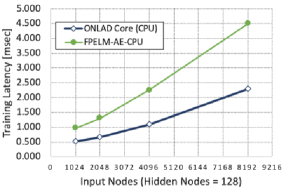
6.2.2 Computational Cost of Proposed Forgetting Mechanism
Here, the proposed forgetting mechanism of ONLAD Core and the baseline algorithm (i.e., FP-ELM) are compared in terms of computational cost. Since the forgetting operation of ONLAD Core or FP-ELM is unified into the training algorithm, we use training latency times to compare them. Also, to make a fair comparison of their computational costs, we compare a CPU implementation of ONLAD Core and FPELM-AE-CPU, both of which are implemented with the same library (i.e., Tensorflow).
Figure 13 shows the experimental results, where the exploration ranges of input and hidden nodes are set to 8x larger than those of Figures 11 and 12, in order to increase the ratio of computation time of the models and make a clear comparison of their computational costs. Consequently, our forgetting mechanism is faster than FPELM-AE-CPU by 3.21x on average. The computational cost of our forgetting mechanism is as shown in Equation 23, however, that of FP-ELM is since the matrix size of the matrix inversion of FP-ELM is ; the gap of their computation times gradually widens as the number of hidden nodes increases.
6.3 FPGA Resource Utilization
This section evaluates FPGA resource utilization of ONLAD Core by varying the numbers of input and hidden nodes. The exploration range of the number of input nodes is chosen to be {128, 256, 512, 1,024}, and that of the number of hidden nodes is to {16, 32, 64} on the basis of the results in the previous section. For ease of analysis, we use pre-synthesis resource utilization reports produced by Vivado HLS as experimental results.
Table 15 shows the experimental results. The DSP utilization remains almost constant even as the numbers of input and hidden nodes increase. This is a reasonable outcome since the DSP slices are consumed only for Train Module and Predict Module, and both of them are designed to use a specific number of arithmetic units regardless of the number of input and hidden nodes, as mentioned in Sections 4.2.3 and 4.2.4.
However, ONLAD Core consumes more BRAM instances as the model size increases. below denotes the total number of matrix elements of the entire ONLAD Core.
| (29) |
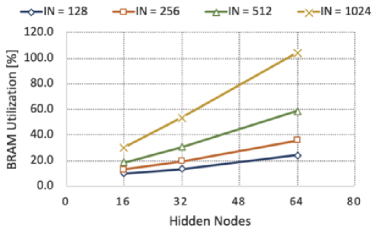
Equation 29 shows that the utilization of the BRAM instances of ONLAD Core is linearly increased as the number of input nodes increases. The experimental results shown in Table 15 are consistent with Equation 29; the BRAM utilization is proportional to the number of input nodes.
Equation 29 also shows that the utilization of the BRAM instances is proportional to the square of the number of hidden nodes , too. However, the BRAM utilization ratios of ONLAD Core are almost proportional to the number of hidden nodes, as shown in Figure 15. The same logic as in the previous section can explain this outcome; holds as long as in Equation 29. The practicality of the condition is also as described in the previous section. Hence, in practical situations, the BRAM utilization of ONLAD Core is suppressed and does not excessively increase even if the number of hidden nodes increases. Consequently, except for the largest setting , all the utilization rates of ONLAD Core are under the limit.
| Hidden Nodes = 16 | ||||
|---|---|---|---|---|
| Input Nodes | BRAM [%] | DSP [%] | FF [%] | LUT [%] |
| 128 | 10.0 | 40.0 | 16.0 | 29.9 |
| 256 | 12.9 | 40.0 | 16.1 | 30.0 |
| 512 | 18.6 | 40.0 | 16.1 | 30.0 |
| 1,024 | 30.0 | 40.0 | 16.1 | 30.0 |
| Hidden Nodes = 32 | ||||
| Input Nodes | BRAM [%] | DSP [%] | FF [%] | LUT [%] |
| 128 | 13.6 | 40.0 | 16.0 | 29.9 |
| 256 | 19.3 | 40.0 | 16.0 | 30.0 |
| 512 | 30.7 | 40.0 | 16.0 | 30.0 |
| 1,024 | 53.6 | 40.0 | 16.0 | 30.0 |
| Hidden Nodes = 64 | ||||
| Input Nodes | BRAM [%] | DSP [%] | FF [%] | LUT [%] |
| 128 | 24.3 | 40.0 | 15.9 | 30.0 |
| 256 | 35.7 | 40.0 | 15.9 | 30.0 |
| 512 | 58.6 | 40.0 | 16.0 | 30.0 |
| 1,024 | 104.2 | 40.0 | 16.0 | 30.1 |
6.4 Power Consumption
This section evaluates the runtime power consumption of our board-level implementation in comparison with the other software implementations. We use an ordinary watt-hour meter to measure the power consumption of PYNQ-Z1 board. For the software implementations, s-tui and nvidia-smi are used. s-tui [37] is an open-source CPU monitoring tool; we use it to measure the power consumption of the CPU (i.e., Intel Core i7 6700 3.4GHz) equipped in the experimental machine. On the other hand, nvidia-smi is a GPU monitoring utility provided by Nvidia. We use it to measure the power consumption of the GPU (i.e., Nvidia GTX 1070 8GB) equipped in the experimental machine.
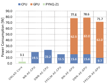
The input and hidden nodes of all the implementations are commonly set to 512 and 64. This setting has been confirmed to consume the largest amount of resources in Table 15. The resource utilization report of ONLAD Core is shown in Table 10.
Figure 16 shows the power consumption of each implementation when training computations are continuously executed. As shown in the figure, our implementation consumes 3.1 W, 5.0x25.4x lower than the others. The reported power consumption of our implementation includes not only that of ONLAD Core, but also that of other components such as a dual-core ARM CPU. Hence, the power consumption of ONLAD Core itself is even lower than 3.1 W.
7 Related Work
7.1 On-device Learning
Data play an important role in machine learning, although sometimes they can be privacy-sensitive. Here, on-device prediction/learning is a way to ensure data privacy because it does not require user data transfers with external server machines. Ravi et al. proposed ProjectionNet [38] to make existing BP-NN-based models smaller and reduce the memory they take up on user devices without significantly degrading accuracy. This is done by leveraging an LSH (Locality Sensitive Hashing) based projection method and a distillation training framework. Konečný et al. proposed a federated learning framework [39], which utilizes user devices as computational nodes to train a global model. In this framework, user devices are supposed to perform training only with their local data; then, the updated weights are aggregated into the global model. Zhu et al. and Park et al. studied federated learning approaches with edge devices on wireless sensor networks [40][41]. They explored their essential building blocks and pointed out underlying challenges. Our approach shares a common idea that edge devices themselves perform training, although the aim is not to create a global model; our work tries to create a locally personalized model for the target edge device.
7.2 Anomaly Detection with OS-ELM
Since sequential learning approaches are capable of learning input data online, they have been utilized for anomaly detection where real-time adaptation and prediction are often required. OS-ELM is no exception; several studies have been reported on anomaly detection using OS-ELM. Nizar et al. proposed an OS-ELM-based irregular behavior detection system of electricity customers to prevent non-technical losses such as power theft and illegal connections [42]. They compared their system with SVM based ones and showed its superiority. Singh et al. proposed an OS-ELM-based network traffic IDS (Intrusion Detection System). They showed that the system can perform training on a huge amount of traffic data even with limited memory space [43]. Bosman et al. proposed a decentralized anomaly detection system for wireless sensor networks [44]. On the other hand, we utilize OS-ELM for semi-supervised anomaly detection in conjunction with an autoencoder. As far as we know, we propose the combination as the first work.
7.3 OS-ELM Variants with Forgetting Mechanisms
Over the past several years, several OS-ELM variants with forgetting mechanisms have been proposed. Zhao et al. were the first to study a forgetting mechanism for OS-ELM, called FOS-ELM [45]. FOS-ELM takes a sliding-window approach, where the latest training chunks are taken into account ( is a fixed parameter of window size). On the other hand, OS-ELM [46] and FP-ELM [26] introduce variable forgetting factors to forget old training chunks gradually. They adaptively update the forgetting factors according to the information in arriving input data or output error values. Our approach is based on FP-ELM, though it is modified to provide the forgetting mechanism with a tiny additional computational cost to the original algorithm of OS-ELM.
| BRAM [%] | DSP [%] | FF [%] | LUT [%] |
| 55.4 | 32.7 | 11.6 | 25.8 |
7.4 Hardware Implementations of OS-ELM
Several papers on hardware implementations of ELM [47][48][49][50] have been reported since 2012. However, implementations of OS-ELM have just started to be reported. Tsukada et al. provided a theoretical analysis for hardware implementations of OS-ELM to significantly reduce the computational cost [18]. Villora et al. and Safaei et al. proposed fast and efficient FPGA-based implementations of OS-ELM for embedded systems [51][52]. In this paper, we propose an IP core that implements the proposed OS-ELM-based semi-supervised anomaly detection approach. This IP core can be implemented on edge devices of limited resources and works at low power consumption.
7.5 Neural Network Based Hardware Implementations for Anomaly Detection
In this section, we compare several NN-based anomaly detection hardware implementations in Table 11. Akin et al. proposed an FPGA based condition monitoring system, whose prediction time is less than 2 msec, for induction motors [53]. The proposed system employs a supervised anomaly detection approach using a 3-layer binary-classification model; it requires both anomaly data and normal data for training. Wess et al. proposed an electrocardiogram anomaly detection approach based on FPGA [54]. The proposed system consists of (1) feature extraction, (2) dimensional reduction, and (3) classification, in which (3) is implemented as a dedicated circuit on FPGA. They reported that the prediction latency is approximately less than 100 cycles, although their approach is also based on a classification model as well as [53]. In contrast to the above implementations, ONLAD Core adopts a semi-supervised approach, where only normal data are required for training.
Moss et al. proposed an FPGA based anomaly detector for radio frequency signals [55]. The proposed IP core realizes semi-supervised anomaly detection using a BP-NN based autoencoder, which is a similar approach to our work. Also, its prediction latency is as fast as 105 nsec. However, the model size (i.e., weight parameters) is 100x smaller than ONLAD Core, and the FPGA platform is much larger than ours. Besides, their IP core does not support training computations. Alrawashdeh et al. proposed a DBN (Deep Belief Network) based IP core that supports training as with ONLAD Core for anomaly detection [56]. They proposed a cost-efficient training model for the contrastive divergence algorithm of DBN and reported that the performance of the IP core achieves 37 Gops/W. However, the model adopts a classification based approach as with [53] and [54]. On the other hand, ONLAD Core supports training, and at the same time it adopts a semi-supervised anomaly detection approach, which makes it more applicable to a wide range of real-world applications.
| Akin et al. [53] | Wess et al. [54] | Moss et al. [55] | Alrawashdeh [56] | ONLAD Core | |||||||||||
|---|---|---|---|---|---|---|---|---|---|---|---|---|---|---|---|
| Approach |
|
|
|
|
|
||||||||||
| NN Model | BP-NN | BP-NN | BP-NN | DBN | OS-ELM | ||||||||||
| Layers | 3 | 3 | 5 | 4 | 3 | ||||||||||
| Weight Parameters |
|
|
|
N/A |
|
||||||||||
| Platform | Altera Cyclone iii Devkit | Avnet Zedboard | Ettus USRP X310 | Xilinx ZC706 | Digilent PYNQ-Z1 | ||||||||||
| Tools | Quartus ii (VHDL) | Vivado (HLS) | Vivado (HLS) | Vivado (Verilog) | Vivado (HLS) | ||||||||||
|
No | No | No | Yes | Yes | ||||||||||
| Frequency | 50 MHz | N/A | 200 MHz | N/A | 100 MHz | ||||||||||
| Prediction Latency | 2 msec | 100 cycles | 105 nsec | 8sec | 1 msec | ||||||||||
| Training Latency | N/A | N/A | N/A | N/A | 1 msec | ||||||||||
| Power Consumption | N/A | N/A | N/A | N/A | 3.1 W | ||||||||||
| Power Efficiency | N/A | N/A | N/A | 37 Gops/W | N/A |
7.6 Design Tools for Hardware Implementation of Neural Networks
The PYNQ-Z1 board used in this work provides the PYNQ library [57] which allows the developers to design CPU-FPGA co-architecture with Python codes, although it is not specialized for implementing neural networks. fpgaConvNet [58] is an automated design framework for CNN (Convolutional Neural Network) based classification models on FPGA platforms. This framework adopts a synchronous dataflow model where the design space of performance and cost is explored, while taking into account platform-specific constraints. DnnWeaver [59] is a design tool that generates synthesizable DNN accelerators from high-level configurations in Caffe. The DnnWeaver compiler tiles, schedules, and batches DNN operations to maximize data reuse and utilize target FPGA’s memory. Zhao et al. proposed a high-level design framework for BNNs (Binarized Neural Networks) [60]. Since the main arithmetics of BNNs are simple bitwise logic operations instead of costly floating-point operations, the computational cost and FPGA resources required to implement the accelerator can be significantly reduced compared with conventional CNNs. GUINNESS [61] is a GUI based design tool for implementing BNNs on Xilinx SoC platforms. In this tool, the designers do not need to write any RTL codes or scripts, which enables software designers to develop prototypes of BNN-based accelerators without knowledge of hardware.
8 Conclusions
8.1 Summary
In this work, we proposed ONLAD which realizes fast sequential learning semi-supervised anomaly detection by constructing an autoencoder with OS-ELM. We showed that the computational cost of OS-ELM is significantly reduced when the batch size is fixed to 1, which contributes to speedup of ONLAD. Also, we proposed a computationally lightweight forgetting mechanism for OS-ELM, based on FP-ELM. It enables ONLAD to follow concept drift at a low computational cost. In addition, we proposed ONLAD Core in order to realize on-device execution of ONLAD on resource-limited edge devices at low power consumption. Since ONLAD Core does not need to offload training computations to external remote server machines, it enables standalone execution where no data transfers to server machines are required.
Experimental results using public datasets showed that ONLAD has comparable generalization capability to that of BP-NN-based models in the context of anomaly detection. We also confirmed that ONLAD has favorable anomaly detection capability especially in an environment that simulates concept drift.
Evaluations of ONLAD Core confirmed that it can perform training and prediction computations faster than software implementations of BP-NNs and FP-ELM by 1.95x6.58x and 2.29x4.73x on average. They also comfirmed that the proposed forgetting mechanism is faster than FP-ELM by 3.21x on average. In addition, our evaluations showed that ONLAD Core can be implemented on PYNQ-Z1 board in practical model sizes. We demonstrated that the runtime power consumption of PYNQ-Z1 board that implements ONLAD Core is 5.0x25.4x lower in comparison with the other software implementations when training computations are continuously executed.
8.2 Future Directions
BP-NNs are known to achieve higher generalization performance to some extent by stacking more layers. Although the original OS-ELM algorithm is limited to have only one hidden layer, ML-OSELM (Multi-Layer Online Sequential Extreme Learning Machine) [62] proposed by Mirza et al. provides a multi-layer framework for OS-ELM. According to [62], ML-OSELM outperforms OS-ELM on well-known open classification datasets by 0.152.58% in terms of test accuracy. Thus, anomaly detection capability of ONLAD can be further improved by replacing OS-ELM in ONLAD with ML-OSELM. We plan to work with the multi-layer version of ONLAD and ONLAD Core.
In real world, there are some systems that have multiple action modes such as air conditioners, robot arms, and gas turbines. In the context of anomaly detection, such systems are often formulated as mixture models which consist of multiple sub-distributions of normal data. Recently, a mixture model framework that utilizes multiple OS-ELM instances was proposed in [63]. We plan to apply this framework to ONLAD and ONLAD Core.
References
- [1] V. Chandola, A. Banerjee, and V. Kumar. Anomaly Detection: A Survey. ACM Computing Surveys, 41(3):1–58, Jul 2009.
- [2] N.V. Chawla, N. Japkowicz, and A. Kolcz. Editorial: Special Issue on Learning from Imbalanced Data Sets. SIGKDD Explorations, 6(1):1–6, Jun 2004.
- [3] D.D. Lewis and W.A. Gale. A Sequential Algorithm for Training Text Classifiers. CoRR, abs/cmp-lg/9407020, 1994.
- [4] A. Estabrooks, T. Jo, and N. Japkowicz. A multiple Resampling Method for Learning from Imbalanced Data Sets. Computational Intelligence, 20(1), Feb 2004.
- [5] M. Pazzani, C. Mertz, P. Murphy, K. Ali, T. Hume, and C. Brunk. In Machine Learning Proceedings, pages 217–225, Jul 1994.
- [6] M.M. Breunig, H.P. Kriegel, R.T. Ng, and J. Sander. LOF: identifying density-based local outliers. In Proceedings of the ACM Special Interest Group on Management of Data, pages 93–104, May 2000.
- [7] Y. Liao and V.R. Vemuri. Use of K-Nearest Neighbor classifier for intrusion detection. Computers & Security, 21(5):439–448, Oct 2002.
- [8] K. Leung and C. Leckie. Unsupervised Anomaly Detection in Network Intrusion Detection Using Clusters. In Proceedings of the Australasian Conference on Computer Science, pages 333–342, Jan 2005.
- [9] G. Münz, S. Li, and G. Carle. Traffic Anomaly Detection Using K-Means Clustering. In Proceedings of the GI/ITG Workshop, pages 13–14, Sep 2007.
- [10] Y. Wang, J. Wong, and A. Miner. Anomaly intrusion detection using one class SVM. In Proceedings of the IEEE SMC Information Assurance Workshop, pages 358–359, Jun 2004.
- [11] K.L. Li, H.K. Huang, S.F. Tian, and W. Xu. Improving one-class SVM for anomaly detection. In Proceedings of the International Conference on Machine Learning and Cybernetics, pages 3077–3081, Nov 2003.
- [12] S.M. Erfani, S. Rajasegarar, S. Karunasekera, and C. Leckie. High-dimensional and large-scale anomaly detection using a linear one-class SVM with deep learning. Pattern Recognition, 58:121–134, Oct 2016.
- [13] M. Sakurada and T. Yairi. Anomaly Detection Using Autoencoders with Nonlinear Dimensionality Reduction. In Proceedings of the Workshop on Machine Learning for Sensory Data Analysis, pages 1–8, Dec 2014.
- [14] T. Schlegl, P. Seeböck, S.M. Waldstein, U.S. Erfurth, and G. Langs. Unsupervised Anomaly Detection with Generative Adversarial Networks to Guide Marker Discovery. In Proceedings of the International Conference on Information Processing in Medical Imaging, pages 146–157, May 2017.
- [15] I. Žliobaitė, M. Pechenizkiy, and J. Gama. An overview of concept drift adaptation. ACM Computing Surveys, 46(4):44:1–44:37, Apr 2014.
- [16] G.I. Webb, M.J. Pazzani, and D. Billsus. Machine Learning for User Modeling. User Modeling and User-Adapted Interaction, 11(1-2):19–29, Mar 2001.
- [17] M. Hind, S. Mehta, A. Mojsilovic, R. Nair, K.N. Ramamurthy, A. Olteanu, and K.R. Varshney. FactSheets: Increasing Trust in AI Services through Supplier’s Declarations of Conformity. CoRR, abs/1808.07261:1–31, Aug 2018.
- [18] M. Tsukada, M. Kondo, and H. Matsutani. OS-ELM-FPGA: An FPGA-Based Online Sequential Unsupervised Anomaly Detector. In Proceedings of the International European Conference on Parallel and Distributed Computing Workshops, pages 518–529, Aug 2018.
- [19] N.Y. Liang, G.B. Huang, P. Saratchandran, and N. Sundararajan. A Fast and Accurate Online Sequential Learning Algorithm for Feedforward Networks. IEEE Transactions on Neural Networks, 17(6):1411–1423, Nov 2006.
- [20] G.E. Hinton and R.R. Salakhutdinov. Reducing the Dimensionality of Data with Neural Networks. Science, 313(5786):504–507, Jul 2006.
- [21] G.B. Huang, Q.Y. Zhu, and C.K. Siew. Extreme Learning Machine: A New Learning Scheme of Feedforward Neural Networks. In Proceedings of the International Joint Conference on Neural Networks, pages 985–990, Jul 2004.
- [22] G.H. Golub and C. Reinsch. Singular value decomposition and least squares solutions. Numerische Mathematik, 14(5):403–420, Apr 1970.
- [23] P. Vincent, H. Larochelle, Y. Bengio, and P.A. Manzagol. Extracting and composing robust features with denoising autoencoders. In Proceedings of the International Conference on Machine Learning, pages 1096–1103, Jul 2008.
- [24] A. Jinwon and C. Sungzoon. Variational autoencoder based anomaly detection using reconstruction probability. Special Lecture on IE, 2:1–18, 2013.
- [25] B. Schölkopf, A. Smola, and K.R. Müller. Kernel Principal Component Analysis. In Proceedings of the International Conference on Artificial Neural Networks, pages 583–588, Jun 2005.
- [26] D. Liu, Y. Wu, and H. Jiang. FP-ELM: An online sequential learning algorithm for dealing with concept drift. Neurocomputing, 207(26):322–334, Sep 2016.
- [27] G.H. Golub and C.F.V. Loan. Matrix Computations. Johns Hopkins University Press, 3rd edition, Oct 1996.
- [28] H. Xiao, K. Rasul, and R. Vollgraf. Fashion-MNIST: a Novel Image Dataset for Benchmarking Machine Learning Algorithms. https://github.com/zalandoresearch/fashion-mnist, 2017.
- [29] Y. Lecun and C. Cortes. MNIST handwritten digit database. http://yann.lecun.com/exdb/mnist/, 2010.
- [30] D. Dua and C. Graff. UCI Machine Learning Repository, 2017.
- [31] G. Cybenko. Approximation by Superpositions of a Sigmoidal Function. Mathematics of Control, Signals and Systems, 2(4):303–314, Dec 1989.
- [32] V. Nair and G. Hinton. Rectified Linear Units Improve Restricted Boltzmann Machines. In Proceedings of the International Conference on Machine Learning, pages 807–814, Jun 2010.
- [33] D.P. Kingma and J. Ba. Adam: A Method for Stochastic Optimization. CoRR, abs/1412.6980:1–15, Dec 2014.
- [34] M. Abadi, P. Barham, J. Chen, Z. Chen, A. Davis, J. Dean, M. Devin, S. Ghemawat, G. Irving, M. Isard, M. Kudlur, J. Levenberg, R. Monga, S. Moore, D.G. Murray, B. Steiner, P. Tucker, V. Vasudevan, P. Warden, M. Wickle, Y. Yu, and X. Zheng. TensorFlow: Large-Scale Machine Learning on Heterogeneous Systems. In Proceedings of the USENIX Conference on Operating Systems Design and Implementation, pages 265–283, March 2016.
- [35] M. McCloskey and N.J. Cohen. Catastrophic Interference in Connectionist Networks: The Sequential Learning Problem. Psychology of Learning and Motivation, 24:109–165, 1989.
- [36] J. Nickolls, I. Buck, M. Garland, and K. Skadron. Scalable Parallel Programming with CUDA. ACM Queue, 6(2):40–53, Apr 2008.
- [37] A. Manuskin. Terminal-based CPU stress and monitoring utility. https://github.com/amanusk/s-tui, 2017.
- [38] S. Ravi. ProjectionNet: Learning Efficient On-Device Deep Networks Using Neural Projections. CoRR, abs/1708.00630:1–12, Aug 2017.
- [39] J. Konečný, H.B. McMahan, D. Rampage, and P. Richtárik. Federated Optimization: Distributed Machine Learning for On-Device Intelligence. CoRR, abs/1610.02527:1–38, Oct 2016.
- [40] G. Zhu, D. Liu, Y. Du, C. You, J. Zhang, and K. Huang. Towards an Intelligent Edge: Wireless Communication Meets Machine Learning. CoRR, abs/1809.00343:1–14, Sep 2018.
- [41] J. Park, S. Samarakoon, M. Bennis, and M. Debbah. Wireless network intelligence at the edge. CoRR, abs/1812.02858:1–32, Dec 2018.
- [42] A.H. Nizar and Z.Y. Dong. Identification and detection of electricity customer behavior irregularities. In Proceedings of the IEEE Power Systems Conference and Exposition, pages 1–10, March 2009.
- [43] R. Singh, H. Kumar, and R.K. Singla. An Intrusion Detection System using Network Traffic Profiling and Online Sequential Extreme Learning Machine. Expert Systems with Applications, 42(22):8609–8624, Dec 2015.
- [44] H.H.W.J. Bosman, G. Iacca, A. Tejada, H.J. Wörtche, and A. Liotta. Spatial Anomaly Detection in Sensor Networks using Neighborhood Information. Information Fusion, 33:41–56, Apr 2016.
- [45] J. Zhao, Z. Wang, and D.S. Park. Online sequential extreme learning machine with forgetting mechanism. Neurocomputing, 87(15):79–89, Jun 2012.
- [46] S.G. Soares and R. Araújo. An adaptive ensemble of on-line Extreme Learning Machines with variable forgetting factor for dynamic system prediction. Neurocomputing, 171(1):693–707, Jan 2016.
- [47] S. Decherchi, P. Gastaldo, A. Leoncini, and R. Zunino. Efficient Digital Implementation of Extreme Learning Machines for Classification. IEEE Transactions on Circuits and Systems II: Express Briefs, 59(8):496–500, Aug 2012.
- [48] T.C. Yeam, N. Ismail, K. Mashiko, and T. Matsuzaki. FPGA Implementation of Extreme Learning Machine System for Classification. In Proceedings of the IEEE Region 10 Conference, pages 1868–1873, Nov 2017.
- [49] J.V.F. Villora, A.R. Muñoz, J.M.M. Villena, M.B. Mompean, J.F. Guerrero, and M. Wegrzyn. Hardware Implementation of Real-time Extreme Learning Machine in FPGA: Analysis of Precision, Resource Occupation and Performance. Computers & Electrical Engineering, 51:139–156, Feb 2016.
- [50] A. Basu, S. Shuo, H. Zhou, M.H. Lim, and G.B. Huang. Silicon spiking neurons for hardware implementation of extreme learning machines. Neurocomputing, 102(15):125–134, Feb 2013.
- [51] J.V.F. Villora, A.R. Muñoz, M.B. Mompean, J.B. Aviles, and J.F.G. Martinez. Moving Learning Machine towards Fast Real-Time Applications: A High-Speed FPGA-Based Implementation of the OS-ELM Training Algorithm. Electronics, 7:1–23, Nov 2018.
- [52] A. Safaei, Q.M.J. Wu, T. Akilan, and Y. Yang. System-on-a-Chip (SoC)-based Hardware Acceleration for an Online Sequential Extreme Learning Machine (OS-ELM). IEEE Trans on Computer-Aided Design of Integrated Circuits and Systems (Early Access), Oct 2018.
- [53] E. Akin, I. Aydin, and M. Karakose. FPGA Based Intelligent Condition Monitoring of Induction Motors: Detection, Diagnosis, and Prognosis. In Proceedings of the IEEE International Conference on Industrial Technology, pages 373–378, April 2011.
- [54] M. Wess, P.D.S. Manoj, and A. Jantsch. Neural network based ECG anomaly detection on FPGA and trade-off analysis. In Proceedings of the IEEE International Symposium on Circuits and Systems, pages 1–4, May 2017.
- [55] D.J.M Moss, D. Boland, P. Pourbeik, and P.H.W. Leong. Real-time FPGA-based Anomaly Detection for Radio Frequency Signals. In Proceedings of the IEEE International Symposium on Circuits and Systems, pages 1–5, May 2018.
- [56] K. Alrawashdeh and C. Purdy. Fast Hardware Assisted Online Learning Using Unsupervised Deep Learning Structure for Anomaly Detection. In Proceedings of the International Conference on Information and Computer Technologies, pages 128–134, May 2018.
- [57] PYNQ: Python Productivity for Zynq, 2016.
- [58] S.I. Venieris and C.S. Bouganis. fpgaConvNet: A Framework for Mapping Convolutional Neural Networks on FPGAs. In Proceedings of the IEEE International Symposium on Field-Programmable Custom Computing Machines, pages 40–47, May 2016.
- [59] H. Sharma, J. Park, E. Amaro, and B. Thwaites. From high-level deep neural models to FPGAs. In Proceedings of the IEEE/ACM International Symposium on Microarchitecture, pages 1–12, Oct 2016.
- [60] R. Zhao, W. Song, W. Zhang, T. Xing, J.H. Lin, M. Srivastava, R. Gupta, and Z. Zhang. Accelerating Binarized Convolutional Neural Networks with Software-Programmable FPGAs. In Proceedings of the ACM/SIGDA International Symposium on Field-Programmable Gate Arrays, pages 15–24, Feb 2017.
- [61] H. Nakahara, H. Yonekawa, T. Fujii, M. Shimoda, and S. Sato. GUINNESS: A GUI Based Binarized Deep Neural Network Framework for Software Programmers. IEICE Transactions on Information and Systems, E102.D(5):1003–1011, May 2019.
- [62] B. Mirza, S. Kok, and F. Dong. Multi-Layer Online Sequential Extreme Learning Machine for Image Classification. In Proceedings of the International Conference on Extreme Learning Machines, pages 39–49, Dec 2015.
- [63] R. Ito, M. Tsukada, M. Kondo, and H.Matsutani. An Adaptive Abnormal Behavior Detection using Online Sequential Learning. In Proceedings of the International Conference on Embedded and Ubiquitous Computing, pages 436–440, Aug 2019.