CMU-01 at the SIGMORPHON 2019 Shared Task on
Crosslinguality and Context in Morphology

Abstract

This paper presents the submission by the CMU-01 team to the SIGMORPHON 2019 task 2 of Morphological Analysis and Lemmatization in Context. This task requires us to produce the lemma and morpho-syntactic description of each token in a sequence, for 107 treebanks. We approach this task with a hierarchical neural conditional random field (CRF) model which predicts each coarse-grained feature (eg. POS, Case, etc.) independently. However, most treebanks are under-resourced, thus making it challenging to train deep neural models for them. Hence, we propose a multi-lingual transfer training regime where we transfer from multiple related languages that share similar typology.

1 Introduction

Morphological analysis Hajic and Hladká (1998); Oflazer and Kuruöz (1994) is the task of predicting morpho-syntactic properties along with the lemma of each token in a sequence, with several downstream applications including machine translation Vylomova et al. (2017), named entity recognition Güngör et al. (2018) and semantic role labeling Strubell et al. (2018). Advances in deep learning have enabled significant progress for the task of morphological tagging Müller and Schuetze (2015); Heigold et al. (2017) and lemmatization Malaviya et al. (2019) under large amounts of annotated data. However, most languages are under-resourced and often exhibit diverse linguistic phenomena, thus making it challenging to generalize existing state-of-the-art models for all languages.

In order to tackle the issue of data scarcity, recent approaches have coupled deep learning with cross-lingual transfer learning Malaviya et al. (2018); Cotterell and Heigold (2017); Kondratyuk (2019) and have shown promising results. Previous works (e.g., Cotterell and Heigold, 2017) combine the set of morphological properties into a single monolithic tag and employ multi-sequence classification. This runs the risk of data sparsity and exploding output space for morphologically rich languages. Malaviya et al. (2018) instead predict each coarse-grained feature, such as part-of-speech (POS) or Case, separately by modeling dependencies between these features and also between the labels across the sequence using a factorial conditional random field (CRF). However, this results in a large number of factors leading to a slower training time (over 24h).

To address the issues of both data sparsity and having a tractable computation time, we propose a hierarchical neural model which predicts each coarse-grained feature independently, but without modeling the pairwise interactions within them. This results in a time-efficient computation (5–6h) and substantially outperforms the baselines. To more explicitly incorporate syntactic knowledge, we embed POS information in an encoder which is shared with all feature decoders. To address the issue of data scarcity, we present two multilingual transfer approaches where we train on a group of typologically related languages and find that language-groups with shallower time-depths (i.e., period of time during which languages diverged to become independent) tend to benefit the most from transfer. We focus on the task of contextual morphological analysis and use the provided baseline model for the task of lemmatization Malaviya et al. (2019).

This paper makes the following contributions:

1. We present a hierarchical neural model for contextual morphological analysis with a shared encoder and independent decoders for each coarse-grained feature. This provides us with the flexibility to produce any combination of features.

2. We analyze the dependencies among different morphological features to inform model choices, and find that adding POS information to the encoder significantly improves prediction accuracy by reducing errors across features, particularly Gender errors.

3. We evaluate our proposed approach on 107 treebanks and achieve +14.76 (accuracy) average improvement over the shared task baseline McCarthy et al. (2019) for morphological analysis.

2 Contextual Morphological Analysis

In this section, we formally define the task (§2.1) and describe our proposed approach (§2.2).

2.1 Task Formulation

Formally, we define the task of contextual morphological analysis as a sequence tagging problem. Given a sequence of tokens $\mathbf{x}=x_{1},x_{2},\cdots,x_{n}$, the task is to predict the morphological tagset $\mathbf{y}=y_{1},y_{2},\cdots,y_{n}$ where the target label $y_{i}$ for a token $x_{i}$ constitutes the fine-grained morpho-syntactic traits {N;PL;NOM;FEM}.

Figure 1: Hierarchical neural model for contextual morphological analysis with independent CRF decoders for each coarse-grained feature $F$. For the model mdcrf+pos, POS embeddings are concatenated to the word and char-level representations as depicted above. This model has $|F|$-1 decoders since POS tagger is run separately as a prior step. mdcrf refers to the above model without POS embeddings having all $|F|$ decoders.

2.2 Our Method

In line with Malaviya et al. (2018), we formulate morphological analysis as a feature-wise sequence prediction task, where we predict the fine-grained labels (e.g N, NOM, …) for the corresponding coarse-grained features $F=${POS,Case,…} as shown in Figure 1. However, we only model the transition dependencies between the labels of a feature. This is done for two reasons: 1) As per Malaviya et al. (2018)’s analysis, the removal of pairwise dependencies led to only a -0.93 (avg.) decrease in the F1 score. We further observe in our experiments that our formulation performs better even without explicitly modeling pairwise dependencies; 2) The factorial CRF model gets computationally expensive to train with pairwise dependencies since loopy belief propagation is used for inference.

Therefore, we propose a feature-wise hierarchical neural CRF tagger Lample et al. (2016); Ma and Hovy (2016); Yang et al. (2016) with independent predictions for each coarse-grained feature for a given time-step, without explicitly modeling the pairwise dependencies.

2.2.1 Hierarchical Neural CRF model

The hierarchical neural CRF model comprises of two major components, an encoder which combines character and word-level features into a continuous representation and a multi-class multi-label decoder. Given an unlabeled sequence $x$, the encoder computes the context-senstive hidden representations for each token $x_{i}$. These representations are shared across $|F|$ independent linear-chain CRFs for inference. We refer to this model as mdcrf.

Decoder:

Our decoder comprises of $|F|$ independent feature-wise CRFs whose objective function is given as follows:

$$p(\mathbf{y}|\mathbf{x})=\prod_{j=1}^{F}p_{f}(\mathbf{y_{f}}|\mathbf{x})$$

$$p_{f}(\mathbf{y_{f}}|\mathbf{x})=\frac{\prod_{t=1}^{n}\psi_{i}(y_{f,t-1},y_{f,t},\mathbf{x},t)}{Z(\mathbf{x})}$$

where $F$ = {POS, Case, Gender,…} is the set of coarse-grained features observed in the training dataset. $p_{f}(\mathbf{y_{f}}|\mathbf{x})$ is a feature-wise CRF tagger with $\psi_{i}(y_{t-1},y_{t},\mathbf{x})=\exp(\mathbf{W_{f}}^{T}_{y_{f,t-1},y_{f,t}}\mathbf{x}_{i}+\mathbf{b_{f}}_{y_{f,t-1},y_{f,t}})$ being the energy function for each feature $f$. During inference the predictions from each feature-wise decoder is concatenated together to output the complete morphological analysis of the sequence $x$.

Encoder:

We adopt a standard hierarchical sequence encoder which is shared among all the $|F|$ feature-wise decoders. It consists of a character-level bi-LSTM that computes hidden representations for each token in the sequence. These subword representations help in capturing information about morphological inflections. To further enforce this signal, we add a layer of self-attention Vaswani et al. (2017) on top of the character-level bi-LSTM. Self-attention provides each character with a context from all the characters in the token. A bi-LSTM modeling layer is added on top of the self-attention layer which produces a token-level representation. These representations are then concatenated with a word embedding vector and fed to another bi-LSTM to produce context sensitive token representations which are then fed to all the $|F|$ CRFs for inference.

2.2.2 Adding Linguistic Knowledge

Part-of-speech (POS) is perhaps the most important coarse-grained feature. Not only is every token annotated for POS, but most other features depend on it. For instance, verbs do not have Case, nouns do not have Tense. In order to leverage these linguistic constraints, we incorporate POS information for each token into our shared encoder. We refer to this variant of the model as mdcrf+pos, as shown in Figure 1.

Since POS tags are not available as input, we first run a separate hierarchical neural CRF tagger for POS alone and use the model predictions as input to the mdcrf+pos. For each token, we encode its predicted POS tag into a continuous representation and concatenate it with the character and word-level token representations. Finally, these concatenated representations are fed to the word-level bi-LSTM and inference is performed using $|F|$-1 decoders, excluding the POS decoder. Going forward, we use this model architecture for all our experiments unless otherwise noted.

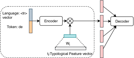
Figure 2: Polyglot model being used for the token “de” in Turkish, denoted by language vector $<$tr$>$.

2.2.3 Multi-lingual Transfer

So far, we have described our model architecture for a monolingual setting. However, the performance of neural models is highly dependent on the availability of large amounts of annotated data, making it challenging to generalize to low-resource languages. Cross-lingual transfer learning attempts to alleviate this challenge by transferring knowledge from high-resource languages. Prior work Cotterell and Heigold (2017); Malaviya et al. (2018); Buys and Botha (2016) has shown the benefits of cross-lingual transfer for morphological tagging. Malaviya et al. (2018) restrict to transferring from one language, whereas Cotterell and Heigold (2017) show that multi-source transfer performs better than single-source. Inspired by this, we experiment with two approaches for multi-lingual transfer learning.

multi-source:

In this method, we augment the training data from related languages with the target language data. Similar to Cotterell and Heigold (2017), we perform a hard clustering of languages based on the typological and orthographic similarity of the source languages with the target language. For instance, we construct a language cluster Indo-Aryan, which comprises of all the languages in the dataset that belong to the Indo-Aryan language family which are Hindi, Marathi and Sanskrit. For some larger language families such as Germanic and Slavic, we construct language clusters from a subset of languages. For instance, the North-Germanic language cluster comprises of treebanks from German, Norwegian, Swedish and Danish. Some languages such as Urdu, Tamil are the only representative languages of their respective language families in the dataset. For these languages, we create a cluster with the next closest language with respect to typology or orthography. For Urdu, we add Hindi because of typological similarity. For other such isolates, we add Turkish because of its extensive agglutination. A total of 24 language clusters were defined based on the literature and with help from a linguist, the details of which can be seen in the Appendix Section §B.

Given a language cluster, all the training data from each language within it is first concatenated together. Then, for each language we concatenate the language embedding vector with the token representation in the encoder by adding the language id $<$lang id$>$ at the beginning and end of each sequence. Given a sequence $\mathbf{x}$, the encoder produces contextualized hidden representation $h_{i}$ for each token $x_{i}$:

$$h_{i}=W_{encoder}(e_{i},c_{i},p_{i},l_{i})$$

where $e_{i}$ is the word embedding vector, $c_{i}$ is the character-level representation, $p_{i}$ is the POS embedding and $l_{i}$ is the language embedding vector. This is done to help the model disambiguate languages as often same tokens have different morpho-syntactic description across languages. For example, the token “” is a part of both Hindi and Marathi vocabulary. In Hindi it denotes a CONJ whereas in Marathi it is a pronoun with the following description: 3;MASC;PRO;NOM;SG.

polyglot:

Languages are often related to multiple languages along different dimensions. For instance, Swedish is lexically similar to German, but it is morpho-syntactically closer to English. To enable a model to utilize these relationships, we feed explicit typological information to the encoder, drawing inspiration from the polyglot model proposed by Tsvetkov et al. (2016). In this multilingual model, we first concatenate all the training data from the source languages, similar to the multi-source setting and compute $h_{i}$ for each token. Then context vector $h_{i}$ is factored by the typology feature vector $t_{l}$ to integrate these manually defined features as follows:

$$f_{l}=\tanh(W_{l}t_{l}+b_{l})$$

$$g_{i}^{l}=h_{i}\otimes f_{l}^{T}$$

where $W_{l},b_{l}$ are language-specific parameters which project the typology vector into a low-dimentional space. Finally, $g_{i}^{l}$ computes the global-context language matrix which is vectorized into a column vector and fed to the decoder, as shown in Figure 2.

Tsvetkov et al. (2016) derive their typology vectors from the URIEL database Littell et al. (2017). We consider a subset of these typology features which are most relevant to the task of morpho-syntactic analysis and obtain 18 Syntax-WALS features. However, we observed that for most language clusters, these typology feature values within a cluster were not discriminating, which defeats the purpose of using polyglot for disambiguating languages across typological dimensions. Therefore, we construct custom typological vector per each language cluster based on the training data global statistics.

For every coarse-grained feature, this constructed vector contains the proportion of words in the training data that are annotated with that feature. We also experiment with calculating these proportions separately for words for each POS label (N, V, …). Given the importance of POS, we also include the number of fine-grained POS labels that the most frequent coarse-grained features (Gender, Number, Person, Case) can take. This results in bi-gram features such as N-FEM, N-NOM, N-SG. We remove features which do not occur within a given cluster to avoid sparse features. Table 1 shows a portion of the example vector constructed for the Indo-Aryan cluster. From the table we can see that, some features such as ADJ-Gender-FEM and V-Person-1 are present in all the three languages within the cluster. Whereas some features such as ADJ-Gender-NEUT is absent from Hindi because Hindi only has two genders which are MASC and FEM.

Feature	Hindi	Marathi	Sanskrit
ADJ-Gender-FEM	0.054	0.144	0.080
V-Person-1	0.004	0.037	0.0736
ADJ-Gender-NEUT	0.0	0.144	0.159
ADJ-Case-DAT/GEN	0.0002	0.0	0.0

Table 1: Example of manually constructed typology features for the Indo-Aryan cluster.

Training Regime:

For both the multi-lingual transfer methods, we train one model per language cluster and fine-tune this model for each individual language. which saves time and compute for training 107 individual models from scratch. Furthermore, since a language cluster can have multiple high-resource languages, we take min (5000, #training data-points) for each language to have a tractable training time. We up-sample the low-resource languages to match the number of training data-points of the high-resource languages.

3 Contextual Lemmatization

We use the neural model from Malaviya et al. (2019) for contextual lemmatization. This is a neural sequence-to-sequence model with hard attention, which takes both the inflected form and morphological tag set for a token as input and produces a lemma, both at the character level. The decoder uses the concatenation of the previous character and the tag set to produce the next character in the lemma. The lemmatization model is jointly trained with an LSTM-based tagger using jackknifing to reduce exposure bias in training: Malaviya et al. (2019) report significantly lower lemmatization results training with gold tags and using predicted tags only at test time. We use their tagger for training and our contextual morphological analysis models’ predicted tags at evaluation time. This model served as the baseline lemmatizer for Task 2; we refer readers to the shared task paper for model details McCarthy et al. (2019).

Language	Model	tgt-size=100			tgt-size=1,000
		Accuracy	F1-Macro	F1-Micro	Accuracy	F1-Macro	F1-Micro
RU/BG	mdcrf + pos + multi-source	69.13	85.78	85.86	82.72	92.15	92.17
	Malaviya et al. (2018)	46.89	64.75	64.46	67.56	82.06	82.11
	Cotterell and Heigold (2017)	52.76	58.23	58.41	71.90	77.89	77.97
FI/HU	mdcrf + pos + multi-source	57.32	80.11	78.86	70.24	85.44	84.86
	Malaviya et al. (2018)	45.41	68.63	68.07	63.93	85.06	84.12
	Cotterell and Heigold (2017)	51.74	68.15	66.82	61.8	75.96	76.16

Table 2: Comparing our model for bilingual transfer with previous baselines.

4 Experiments

We conduct the following experiments: We compare our multi-lingual transfer approach with the baselines Malaviya et al. (2018) and Cotterell and Heigold (2017) under the same experimental settings. Next, we compare our approach with the shared task baseline McCarthy et al. (2019). Finally, we analyze the contributions of different components of our proposed method.

Baselines:

Cotterell and Heigold (2017) formulate this task as a sequence prediction problem with the output space being the set of all possible tagsets seen in the training data. Specifically, they construct a neural network based multi-class classifier where each tagset {N;PL;NOM;FEM} forms a class. Since the output space is only restricted to the tagsets seen in the training data, this method cannot generalize to unseen tagsets. Furthermore, for morphologically rich languages such as Russian or Turkish, the output space of the tagset is huge leading to sparse training data. McCarthy et al. (2019) follow a similar approach.

To overcome these drawbacks Malaviya et al. (2018) consider a feature-wise model which predicts fine-grained labels for corresponding coarse categories {POS,Case,…}. Since morpho-syntactic properties are often correlated, they model these inter-dependencies using a factorial CRF and define two inter-dependencies: 1) a pairwise dependency, which models correlations between the morpho-syntactic properties within a token, and 2) a transition dependency, which models label correlations across all tokens in a sequence. Although this formulation provides the flexibility to produce any combination of tagsets, this model is computationally expensive to train since the factors model dependencies between all labels of all coarse-grained features, leading to >20k factors.

Data processing:

We use the train/dev/test split provided in the shared task McCarthy et al. (2018). Since we model feature-wise prediction for each coarse-grained feature, our model requires the provided data to be annotated for coarse-grained features. Therefore, we construct a feature-label dictionary based on the UM documentation to map the individual fine-grained traits, which are in the UM schema, to their respective coarse-grained categories. This transforms the tagset {N;PL;NOM;FEM} as {POS=N;Number=PL;Case=NOM;Gender=FEM}. We note that usually a token has a subset of the coarse-grained categories, therefore we extend the morphological tagset for each token by adding the remaining features observed in the training set and assigning them a special value “_” which denotes null.

Hyper-parameters:

We use a hidden size of 200 for each direction of the LSTM with a dropout of 0.5. For the character-level bi-LSTM we use a hidden size of 25. We use 100 dimentional size for word and language embeddings with 64 dimensional POS embeddings, all randomly initialized. SGD was used as the optimizer with learning rate of 0.015. The models were trained until convergence. For Polyglot, we project the constructed typology vector into 20 dimension hidden size.

5 Results and Discussion

Table 2 shows the comparison results of our proposed approach with the baselines Malaviya et al. (2018); Cotterell and Heigold (2017) using cross-lingual transfer. Here mdcrf+pos refers to our model architecture and multi-source refers to our multi-lingual transfer approach. Malaviya et al. (2018) and Cotterell and Heigold (2017) test their approach on UD v2.1 Nivre et al. (2017) under two settings: tgt size $=100$ and tgt size $=1000$, where tgt size denotes the number of target language data-points used during training. Malaviya et al. (2018) transfer from one related high-resource language. We use the same experimental resources for comparison and for a fair comparison we do not fine-tune on the target language. Of the four language pairs tested by Malaviya et al. (2018), we choose RU/BG and FI/HU for comparison, where BG and HU are the target languages and RU and FI are the respective transfer languages, since these languages are morphologically challenging. We see that under both settings our approach outperforms the baselines by a significant margin for both the language pairs.

Next, we compare our multi-lingual transfer approaches multi-source and multi-source + polyglot in order to decide the model for our final submission. We conduct experiments on three low-resource languages: Marathi (mr-ufal), Sanskrit (sa-ufal) and Belarusian (be-hse), all of which have $<400$ training data-points. The italicized text denotes the treebank used in the experiments. For mr-ufal and sa-ufal, we transfer from a related high-resource language of Hindi (hi-hdtb). For be-hse, we transfer from two related languages, Russian (ru-gsd) and Ukrainian (uk-iu). However, from Table 3, we see that the performance of the two models is comparable. Therefore, for our final submission we use only multi-source which is much faster to train than the multi-source + polyglot. We discuss their comparative performance in greater detail in Section §5.1.

Model	mr-ufal	sa-ufal	be-hse
multi-source	63.52 / 78.22	42.78 / 67.64	77.07 / 82.89
+polyglot	61.18 / 77.42	43.81 / 65.94	76.51 / 83.27

Table 3: Multi-lingual comparison results for Marathi (mr-ufal), Sanskrit (sa-ufal) and Belarusian (be-hse) on the validation set.

Finally, we compare our approach with the shared task baseline. Table 5, 6 in the Appendix shows our results for all 107 treebanks. We observe that out system achieves an average improvement of +14.70 (accuracy) and +4.63 (F1) over the provided baseline McCarthy et al. (2019). We note that for the shared task submission, we did not use self-attention over the character-level representations. Therefore, we additionally show the results after adding self-attention. We observe that the addition gives an average improvement of +0.60 (accuracy) and +0.30 (F1) over our previous best submission.

5.1 Analysis

Here we analyze the different components of our model in an effort to understand what it is learning.

Why does adding POS help?

As discussed earlier (§2), we explicitly add the POS feature in the form of embeddings into the shared encoder. To evaluate the contribution of POS alone, we conduct monolingual experiments without concatenating the POS embeddings with the token-level representations. Table 4 outlines the ablation results for three treebanks with varying training size. We observe that our monolingual model mdcrf significantly outperforms the baseline McCarthy et al. (2019) by +13.72 accuracy and +3.82 F1 (avg). On adding POS, we further gain +3.56 accuracy and +0.71 F1 over mdcrf across the three treebanks. We note that this improvement is more pronounced for the low-medium resource languages of Marathi (+6.12 accuracy) and Ukrainian (+3.57 accuracy).

Model	mr-ufal	uk-iu	hi-hdtb
MDCRF+POS	64.71 / 79.40	84.79 / 92.03	90.46 / 96.69
MDCRF	58.59 / 77.91	81.22 / 91.35	89.45 / 96.73
McCarthy et al. (2019)	43.76 / 73.38	63.36 / 87.01	80.96 / 94.14

Table 4: Ablation results for Marathi (mr-ufal), Ukrainian (uk-iu) and Hindi (hi-hdtb) with training size of 373, 5441, 13381 respectively on the validation set.

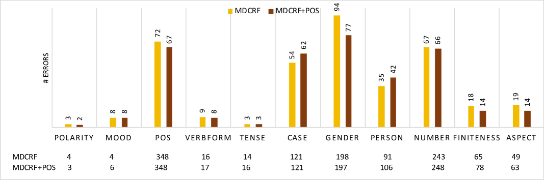
Figure 3: Number of errors per coarse-grained feature for Marathi comparing the addition of POS to the encoder. The rows at the bottom denote the total number of predictions per each feature for both the models.

To understand where the addition of POS helps, we analyse the number of errors made per each coarse-grained feature. For the example of Marathi, POS helped the most in reducing Gender errors (Figure 3). For some word forms, the gender may be inferred from inflectional form alone, but for others, this information may be insufficient, e.g. “” (price.N.FEM.SG.ACC) in Marathi which does not have the traditional female suffix “”. We observe that this behavior corresponds to POS: verbs and adjectives are more predictable from surface forms alone than nouns. The addition of POS information in the encoder helps the model learn to weigh different encoded information more heavily when assigning gender to different parts of speech. For Ukrainian and Sanskrit, POS information also helped reduce errors in Case and Number. More details can be found in Appendix Section §C.

Tkachenko and Sirts (2018) also model dependence on POS with a POS-dependent context vector in the decoder. However, they observe no significant improvement; we hypothesize that incorporating POS information into the shared encoder instead provides the model with a stronger signal.

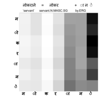
(a) Marathi

(b) Indonesian

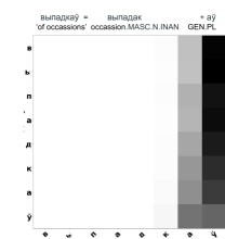
(c) Belarusian

Figure 4: Character-level attention maps for three typologically different languages. Marathi and Belarusian display morphological inflections pre-dominantly as suffix. Indonesian displays inflections in the form of prefix, suffix and circumfix where the affix is found both at the beginning and end of a token.

What is the model learning?

One of the major advantages of our model’s use of self-attention is that it enables us to provide insights into what the model has learned. As seen in Figure 4, we found evidence of the model learning language-specific inflectional properties. Both Marathi and Belarusian display morphological inflections predominantly in the form of suffix and the attention maps for both these languages demonstrate the same. For the Marathi example, the last three characters denote the ergative case and we can see that the attention weights are concentrated on these three characters. Similarly for the Belarusian example, the last two characters denote the genitive case with plural number and is the focus of the attention. For Indonesian, inflections can be also found as circumfixes where the affix is attached at both the beginning and end of the token. For instance, both ke- and -an affixes are appended to form nouns and we can see from Figure 4 that the attention is focused both on the prefix and the suffix. Interestingly for Indonesian, the model seems to have also discovered the stem camat, as evidenced from the attention pattern.

Does time-depth matter for transfer learning?

As discussed earlier, we train one model per language cluster for multi-lingual transfer learning. We compare different clusters to see if time-depth of the languages within a cluster affects the extent of transfer. Time depth is the period of time that has elapsed since all languages in the group were a single language (in other words, the time since divergence). We consider the following three clusters: Hindi-Marathi-Sanskrit (Indo-Aryan), Russian-Ukrainian-Belarusian (Slavic) and Arabic-Hebrew-Amharic-Akkadian (Semitic). These three clusters were chosen because the languages in them became separate languages at varying time-depths. For instance, in the Semitic cluster the languages diverged roughly 5000 years ago, whereas for the Slavic cluster the time-depth is $<$1000 years. Therefore, we expect transfer to help more for languages where the time-depth is more recent. In Figure 5, we compare the multi-source model with our best mono-lingual model mdcrf+pos and we see that transfer helps most for the Slavic cluster by +2.9 accuracy. For the Indo-Aryan cluster it helps by +0.32 accuracy and for the Semitic cluster we observe a slight negative effect with transfer (-0.0176 accuracy). This supports our hypothesis that time-depth does affect the extent of transfer learning with language clusters having lower time-depths benefiting the most.

One particular advantage that the Slavic cluster has over both the Indo-Aryan and Semitic clusters is the similarity of script. Russian, Belarusian, and Ukrainian use variants of the same script; Hindi, Sanskrit, and Marathi do, as well, but the Semitic languages all use different scripts. This is also attributed to the shallower time-depths of the Slavic and Indo-Aryan clusters. Therefore, as suggested by the anonymous reviewers, we add Czech and Polish to the Slavic cluster and see to what extent the scripts are confusing the model. Czech and Polish use different script as compared to Russian, Belarusian, and Ukrainian. We observe that multi-source model like before, achieves similar improvements over the monolingual models for Belarusian (+8.17 accuracy) and Ukrainian (+1.2 accuracy). However, a slight decrease is observed for Russian ( -0.45 accuracy). This suggests that the multi-source model is robust to scriptal changes and benefits the low-resource languages by learning from typologically similar languages, more so for language clusters with shallow time-depths.

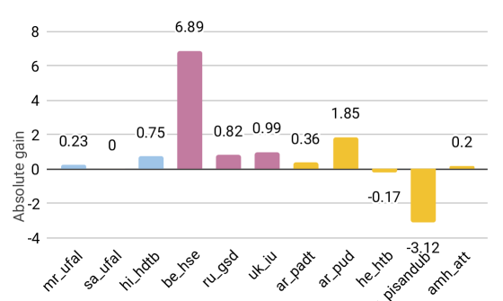
Figure 5: Absolute gain of multi-lingual transfer over monolingual models. Blue denotes the Indo-Aryan cluster, pink the Slavic, and yellow the Semitic.

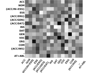
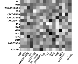
Figure 6: Transition weights for the Case feature for Hindi across multi-source (left) and multi-source + polyglot (right) models trained with Hindi (hi-hdtb), Marathi (mr-ufal) and Sanskrit (sa-ufal).

Why did polyglot not help further?

We hypothesize that one reason why polyglot did not help over multi-source is because the language embedding vector probably learns the same typological information which the typology vector encodes. Hence, the typological vector doesn’t seem to add any new information. As evidence, we look at the transition weights learned in both the models; as shown in Figure 8, we see that the transition weights learned for the Case feature are very similar for both multi-source and multi-source + polyglot. In the future, we plan to explore the contextual parameter generation method Platanios et al. (2018) for leveraging the typology vectors to inform the decoders during inference.

5.2 Error Analysis

In this section, we analyze the major error categories for the multi-source model for the Indo-Aryan cluster. We observe that Gender, Case, Number, Person features account for the most number of errors (65% for Marathi, 49% for Sanskrit). One reason for this is the non-overlapping output label space across the languages within a cluster. For instance, in the Indo-Aryan cluster, Hindi is a high-resource language ($>13k$ training sentences) with Marathi (373) and Sanskrit (184) being the low-resource languages. We observe that the label space for Case, Gender, Number overlap the least among the three languages. Marathi and Sanskrit have three genders: NEUT, FEM, MASC whereas Hindi only has FEM, MASC. Furthermore, only two Hindi Case labels (ACC, NOM) overlap with Marathi and Sanskrit because in Hindi the labels often have alternatives such as ACC/ERG, ACC/DAT. These differences in the output space negatively affect the transfer. For the Slavic cluster, we observe that almost all the feature labels overlap nicely for the languages therein, which is probably another reason why we see a gain of +6.89 for Belarusian in Figure 5 and only +0.32 increase for Marathi.

We also note that for some languages such as Belarusian and Russian, the POS errors increased by 25.3% and 4.4% respectively for the mdcrf+pos model. This suggests that decoupling POS feature from the other feature decoders harmed the model. In future, we plan to improve the mdcrf+pos model by jointly training POS decoder with the other feature decoders which use the latent representation of POS in an end-to-end fashion.

6 Conclusion and Future Work

We implement a hierarchical neural model with independent decoders for each coarse-grained morphological feature and show that incorporating POS information in the shared encoder helps improve prediction for other features. Furthermore, our multi-lingual transfer methods not only help improve results for related languages but also eliminate the need of training individual models for each dataset from scratch. In future, we plan to explore the use of pre-trained multi-lingual word embeddings such as BERT Devlin et al. (2019), in our encoder.

Appendix

Appendix A Comprehensive Results

Table 5 and 6 document the comprehensive results of our submissions. multi-source was our previous submission to the shared task. We conducted additional experimentas with the addition of self-attention and also report the results for multi-source+self-attention. We report both the accuracy and F1 metric.

Language	Target	multi-source	multi-source	McCarthy et al. (2019)	# Training
Cluster		+ Self-Attention			Sentences
		Accuracy / F1	Accuracy / F1	Accuracy / F1
armenian	UD-Armenian-ArmTDP	83.74 / 88.54	83.83 / 88.17	- / -	825
austronesian	UD-Indonesian-GSD	90.05 / 93.13	90.01 / 93.11	71.49 / 86.02	4475
baltic	UD-Latvian-LVTB	89.0 / 93.04	89.0 / 93.08	70.21 / 89.53	7937
	UD-Lithuanian-HSE	70.29 / 76.38	68.08 / 74.56	43.13 / 67.41	211
celtic	UD-Breton-KEB	85.97 / 88.78	85.07 / 88.07	77.41 / 88.58	711
	UD-Irish-IDT	76.75 / 84.1	76.5 / 84.11	67.45 / 81.72	817
dravidian	UD-Tamil-TTB	82.92 / 89.91	82.48 / 89.77	75.64 / 90.23	481
egyptian	UD-Coptic-Scriptorium	92.02 / 95.28	92.17 / 95.33	87.99 / 93.78	673
germanic	UD-Afrikaans-AfriBooms	96.92 / 97.37	96.94 / 97.35	84.05 / 92.32	1548
	UD-Dutch-Alpino	94.85 / 95.69	94.35 / 95.4	82.15 / 91.26	10867
	UD-Dutch-LassySmall	93.48 / 94.08	93.53 / 94.2	76.24 / 88.13	5873
	UD-English-EWT	94.08 / 95.46	93.9 / 95.4	79.19 / 90.46	13298
	UD-English-GUM	93.44 / 94.38	93.56 / 94.47	79.63 / 90.04	3520
	UD-English-LinES	94.37 / 95.19	93.75 / 94.93	81.03 / 90.99	3652
	UD-English-ParTUT	92.01 / 92.69	91.95 / 92.61	79.57 / 89.04	1673
	UD-English-PUD	89.41 / 91.42	89.8 / 91.6	78.85 / 88.8	801
	UD-Faroese-OFT	80.6 / 89.27	77.52 / 87.87	67.11 / 87.27	967
	UD-Gothic-PROIEL	84.53 / 92.93	83.0 / 92.47	83.01 / 91.3	4321
north-	UD-German-GSD	83.72 / 92.73	82.82 / 92.5	- / -	12473
germanic	UD-Danish-DDT	91.78 / 93.72	91.34 / 93.61	77.89 / 90.89	4410
	UD-Norwegian-Nynorsk	94.39 / 96.35	94.29 / 96.33	71.8 / 88.16	14061
	UD-Norwegian-NynorskLIA	93.03 / 94.55	93.75 / 94.89	- / -	1117
	UD-Swedish-LinES	89.92 / 93.61	89.62 / 93.59	77.97 / 91.02	3652
	UD-Swedish-PUD	87.72 / 90.01	87.13 / 89.8	77.78 / 89.32	801
hellenic	UD-Ancient-Greek-Perseus	84.79 / 92.1	84.27 / 91.88	- / -	11136
	UD-Ancient-Greek-PROIEL	88.1 / 95.55	86.01 / 94.67	- / -	13665
	UD-Greek-GDT	91.15 / 96.23	90.73 / 96.0	78.14 / 93.49	2017
indo-iranian	UD-Urdu-UDTB	77.77 / 92.12	78.05 / 92.16	67.99 / 88.42	4105
indoaryan	UD-Hindi-HDTB	90.76 / 96.77	91.05 / 96.85	80.96 / 94.14	13318
	UD-Marathi-UFAL	57.99 / 73.54	57.72 / 73.04	43.76 / 73.38	373
	UD-Sanskrit-UFAL	43.72 / 64.9	46.73 / 68.08	44.33 / 68.34	185
isolate	UD-Basque-BDT	75.2 / 88.07	75.14 / 87.91	67.61 / 87.63	7195
italic	UD-Latin-ITTB	94.57 / 97.26	94.25 / 97.11	77.62 / 93.19	16809
	UD-Latin-Perseus	76.17 / 86.32	75.76 / 85.92	53.23 / 77.5	1819
	UD-Latin-PROIEL	86.78 / 94.39	86.18 / 94.19	82.27 / 91.38	14721
jako	UD-Japanese-GSD	96.8 / 96.4	96.8 / 96.4	85.25 / 90.31	6557
	UD-Japanese-Modern	95.27 / 95.32	95.27 / 95.32	94.29 / 95.2	658
	UD-Japanese-PUD	95.94 / 95.44	95.94 / 95.44	84.73 / 89.63	801
	UD-Komi-Zyrian-IKDP	51.56 / 61.03	51.56 / 62.27	33.73 / 62.59	70
	UD-Komi-Zyrian-Lattice	53.85 / 64.85	54.4 / 65.23	45.6 / 70.61	153
	UD-Korean-GSD	92.56 / 91.68	92.56 / 91.68	80.18 / 86.08	5072
	UD-Korean-Kaist	95.54 / 94.99	95.54 / 94.99	84.32 / 89.4	21891
	UD-Korean-PUD	84.27 / 89.02	84.46 / 89.28	81.6 / 91.15	801
	UD-Kurmanji-MG	80.82 / 87.79	80.82 / 87.81	70.2 / 85.85	604
niger-congo	UD-Bambara-CRB	91.65 / 94.76	92.41 / 94.86	78.86 / 89.41	821
	UD-Naija-NSC	94.56 / 92.71	94.56 / 92.71	68.66 / 78.96	759
	UD-Yoruba-YTB	93.41 / 93.88	93.8 / 94.19	71.2 / 81.83	81
persian	UD-Persian-Seraji	96.15 / 96.85	95.95 / 96.69	- / -	4798
phillipine	UD-Tagalog-TRG	83.78 / 92.09	83.78 / 92.75	44.0 / 69.31	45
sinotibetan	UD-Cantonese-HK	89.64 / 86.82	89.64 / 86.82	70.15 / 77.76	521
	UD-Chinese-CFL	88.65 / 86.96	88.65 / 86.96	74.65 / 79.91	361
	UD-Chinese-GSD	90.83 / 90.54	90.9 / 90.56	76.81 / 84.35	3998
	UD-Vietnamese-VTB	90.1 / 88.84	90.1 / 88.84	70.71 / 79.01	2401
semitic	UD-Akkadian-PISANDUB	79.21 / 78.65	79.21 / 78.65	84.0 / 84.19	81
	UD-Amharic-ATT	87.24 / 91.13	86.58 / 90.91	76.0 / 88.16	860
	UD-Arabic-PADT	91.77 / 95.44	91.52 / 95.36	77.03 / 92.03	6132
	UD-Arabic-PUD	77.63 / 89.06	77.89 / 89.0	63.81 / 86.29	801
	UD-Hebrew-HTB	94.33 / 95.81	94.03 / 95.65	81.59 / 91.84	4973

Table 5: Comprehensive results

Cluster	Target	multi-source	multi-source	McCarthy et al. (2019)	# Training
		+ Self-Attention			Sentences
		Accuracy / F1	Accuracy / F1	Accuracy / F1
turkic	UD-Turkish-IMST	85.68 / 90.64	85.02 / 90.43	62.04 / 85.33	4509
	UD-Turkish-PUD	79.78 / 90.88	79.33 / 90.54	66.92 / 88.05	801
romance	UD-Catalan-AnCora	textbf96.68 / 98.26	96.63 / 98.24	85.77 / 95.7	13343
	UD-French-GSD	96.19 / 97.51	95.76 / 97.32	84.44 / 94.81	13074
	UD-French-ParTUT	93.04 / 96.05	93.04 / 96.12	81.32 / 92.08	817
	UD-French-Sequoia	95.08 / 96.95	94.96 / 96.96	82.64 / 93.42	2480
	UD-French-Spoken	96.05 / 96.08	96.05 / 96.08	94.57 / 94.85	2229
	UD-Galician-CTG	96.65 / 96.31	96.66 / 96.32	87.23 / 91.81	3195
	UD-Galician-TreeGal	89.69 / 93.2	89.3 / 93.25	76.85 / 90.05	801
	UD-Italian-ISDT	95.91 / 97.24	95.96 / 97.27	83.62 / 94.34	11334
	UD-Italian-ParTUT	95.0 / 96.39	94.87 / 96.39	84.03 / 93.42	1673
	UD-Italian-PoSTWITA	92.13 / 93.13	92.03 / 93.02	70.23 / 88.18	5371
	UD-Italian-PUD	87.55 / 92.4	87.38 / 92.46	80.89 / 92.66	801
	UD-Portuguese-Bosque	92.28 / 95.57	92.06 / 95.5	63.14 / 86.12	7493
	UD-Portuguese-GSD	97.33 / 97.54	97.33 / 97.54	- / -	9663
	UD-Romanian-Nonstandard	91.13 / 95.33	91.07 / 95.29	74.31 / 91.5	8056
	UD-Romanian-RRT	94.67 / 96.58	94.82 / 96.63	81.45 / 93.96	7620
	UD-Spanish-AnCora	96.97 / 98.25	96.86 / 98.22	84.27 / 95.3	14145
	UD-Spanish-GSD	94.05 / 97.08	94.07 / 97.1	- / -	12811
slavic	UD-Belarusian-HSE	79.63 / 85.37	77.28 / 84.11	54.99 / 79.07	315
	UD-Bulgarian-BTB	94.22 / 96.44	93.99 / 96.37	79.75 / 93.91	8911
	UD-Buryat-BDT	78.85 / 81.24	75.96 / 78.66	63.26 / 78.53	742
	UD-Old-Church-Slavonic-PROIEL	87.22 / 94.13	86.94 / 94.03	82.86 / 90.34	5070
	UD-Russian-GSD	84.26 / 91.91	83.25 / 91.55	64.42 / 88.77	4025
	UD-Russian-PUD	76.77 / 87.55	77.25 / 87.49	63.15 / 85.52	801
	UD-Russian-SynTagRus	91.65 / 95.96	92.74 / 96.5	73.9 / 92.84	49512
	UD-Russian-Taiga	74.14 / 80.23	75.24 / 81.25	52.99 / 78.71	1412
	UD-Ukrainian-IU	86.02 / 92.41	85.33 / 92.2	63.36 / 87.01	5441
	UD-Upper-Sorbian-UFAL	74.04 / 82.45	70.12 / 81.21	55.66 / 78.3	517
ugric	UD-Estonian-EDT	87.71 / 94.58	88.47 / 94.93	74.56 / 91.71	24579
	UD-Finnish-FTB	83.24 / 90.38	83.63 / 90.7	73.16 / 89.51	14979
	UD-Finnish-PUD	77.05 / 86.33	77.49 / 86.77	71.65 / 88.87	801
	UD-Hungarian-Szeged	80.57 / 90.88	79.16 / 90.13	63.72 / 87.29	1441
	UD-North-Sami-Giella	84.35 / 88.8	83.78 / 88.65	67.04 / 85.6	2498
	UD-Norwegian-Bokmaal	94.97 / 96.68	94.58 / 96.51	81.44 / 93.19	16037
	UD-Swedish-Talbanken	93.94 / 96.01	93.64 / 95.9	- / -	4821
	UD-Finnish-TDT	86.51 / 92.63	85.55 / 92.2	75.13 / 90.92	12109
westslavic	UD-Croatian-SET	87.23 / 94.04	86.88 / 93.91	72.71 / 90.99	7112
	UD-Czech-CAC	90.66 / 96.72	91.38 / 96.99	77.15 / 93.92	19768
	UD-Czech-CLTT	91.29 / 96.15	91.07 / 96.22	73.92 / 92.37	901
	UD-Czech-FicTree	90.05 / 95.42	90.0 / 95.49	68.28 / 90.37	10209
	UD-Czech-PDT	89.78 / 96.37	54.13 / 73.56	76.69 / 94.28	70331
	UD-Czech-PUD	75.65 / 88.19	77.72 / 89.37	59.54 / 85.5	801
	UD-Polish-LFG	87.76 / 93.7	87.81 / 93.65	- / -	13797
	UD-Polish-SZ	82.27 / 91.38	81.01 / 90.88	65.58 / 88.29	6582
	UD-Serbian-SET	91.89 / 95.46	91.35 / 95.29	75.73 / 91.19	3113
	UD-Slovak-SNK	85.59 / 93.12	84.99 / 92.83	64.24 / 88.16	8484
	UD-Slovenian-SSJ	89.05 / 94.03	87.92 / 93.55	73.73 / 89.95	6401
	UD-Slovenian-SST	85.13 / 90.16	85.51 / 90.02	73.4 / 84.74	2551

Table 6: Comprehensive results

Appendix B Language Clusters

We train one model per language cluster for the multi-lingual transfer learning. Each language cluster was constructed based on the typological and orthographic similarity of the languages therein. Table 5, 6 show details of the language clusters. Figure 7 shows clusters graphically by relative size per dataset.

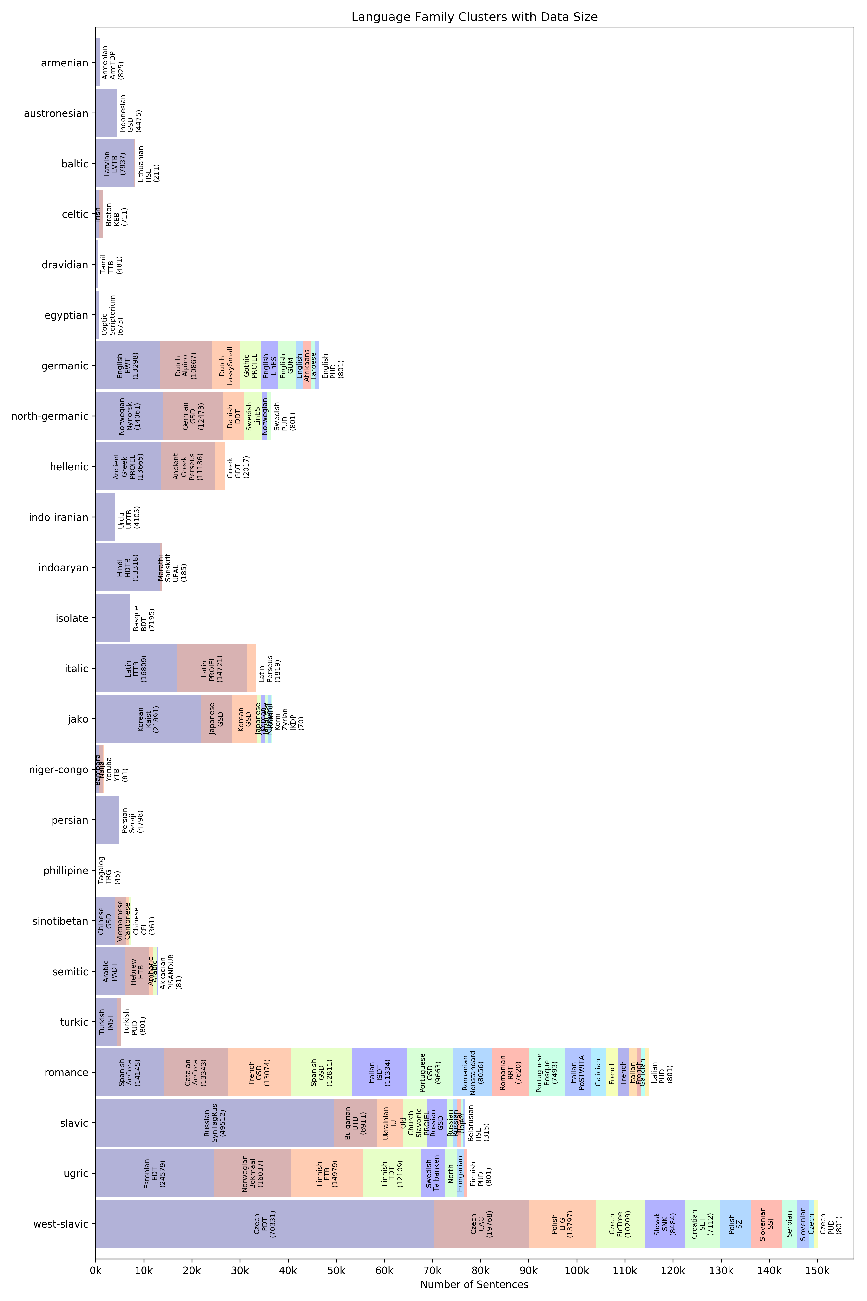
Figure 7: Language family clusters, by number of sentences per dataset.

Appendix C Analysis

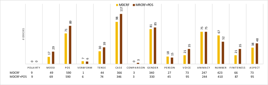
(a) Belarusian (be-hse)

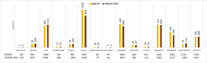
(b) Ukrainian (uk-iu)

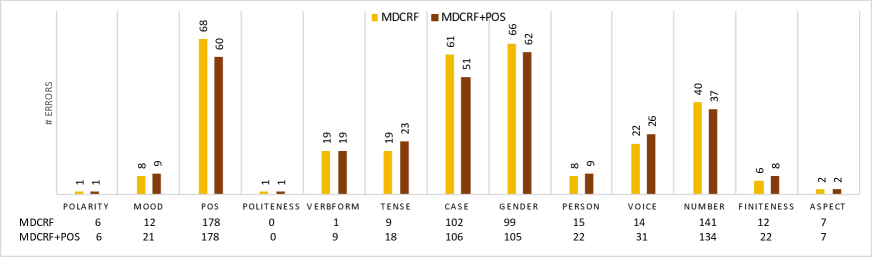
(c) Sanskrit (sa-ufal)

Figure 8: Number of errors per coarse-grained feature for models comparing the addition of POS to the encoder. The rows at the bottom denote the total number of predictions per each feature for both the models.

In order to understand where the addition of POS helps, we plot the number of errors per each coarse-grained feature for three languages in Figure 8. For Sanskrit and Ukrainian we see that POS generally helps reduce the errors predominantly for the features: Case, Gender, Number. For Belarusian, we did not observe a clear trend since the POS accuracy actually decreased for mdcrf+pos.

References

- Buys and Botha (2016) Jan Buys and Jan A. Botha. 2016. Cross-lingual morphological tagging for low-resource languages. In Proc. of ACL, pages 1954–1964.