Leading- and next-to-leading order semiclassical approximation to the first seven virial coefficients of spin-1/2 fermions across spatial dimensions

Abstract

Following up on recent calculations, we investigate the leading- and next-to-leading order semiclassical approximation to the virial coefficients of a two-species fermion system with a contact interaction. Using the analytic result for the second-order virial coefficient as a renormalization condition, we derive expressions for up to the seventh-order virial coefficient $\Delta b_{7}$. Our results at leading order, though approximate, furnish simple analytic formulas that relate $\Delta b_{n}$ to $\Delta b_{2}$ for arbitrary dimension, providing a glimpse into the behavior of the virial expansion across dimensions and coupling strengths. As an application, we calculate the pressure and Tan’s contact of the 2D attractive Fermi gas and examine the radius of convergence of the virial expansion as a function of the coupling strength.

I Introduction

In a recent paper ShillDrut , two of us presented results for virial coefficients in a semiclassical lattice approximation (SCLA), at leading order (LO), for spin-$1/2$ fermions with a contact two-body interaction. We found that, in spite of the crudeness of the approximation, the results for $\Delta b_{3}$ and $\Delta b_{4}$ were surprisingly good when written in terms of the exact $\Delta b_{2}$, which amounted to using the latter as a renormalized coupling. Specifically, quantitative or at least qualitative agreement was found between the LO-SCLA and diagrammatic and Monte Carlo results for 1D and 2D Fermi gases with attractive interactions.

In this work, we explore the LO-SCLA further by carrying out the evaluation of virial coefficients up to $b_{7}$, and furthermore extending our previous analysis to next-to-leading order (NLO). Our (approximate) analytic answers, obtained partially by algebra automation, provide insight into the behavior of the virial expansion as a function of the spatial dimension of the problem. As an application, we compare with Monte Carlo results for the density equation of state of an attractive 2D Fermi gas. As an additional example, we calculate the many-body contribution to Tan’s contact for the same system.

II Hamiltonian and virial expansion

We assume a non-relativistic kinetic energy and a two-body contact interaction, such that the Hamiltonian for two flavors $\uparrow,\downarrow$ is $\hat{H}=\hat{T}+\hat{V}$, where

$$\hat{T}\!=\!{\int{d^{d}x\,\hat{\psi}^{\dagger}_{s}({\bf x})\left(-\frac{\hbar^{2}\nabla^{2}}{2m}\right)\hat{\psi}_{s}({\bf x})}},$$ (1)

and

$$\hat{V}\!=\!-g_{d}\!\int{d^{d}x\,\hat{n}_{\uparrow}({\bf x})\hat{n}_{\downarrow}({\bf x})},$$ (2)

where the field operators $\hat{\psi}_{s},\hat{\psi}^{\dagger}_{s}$ are fermionic fields for particles of spin $s=\uparrow,\downarrow$ (summed over $s$ above), and $\hat{n}_{s}({\bf x})$ are the coordinate-space densities. In the remainder of this work, we will take $\hbar=k_{\text{B}}=m=1$ and discretize spacetime using the spatial lattice spacing $\ell$ to set the scale for all quantities. In particular, we will define the lattice kinetic energy exactly as above by using a momentum-space representation with periodic boundary conditions (rather than a local three-point formula for the second derivative in coordinate space), and the lattice potential energy will take the form

$$\hat{V}\!=\!-g_{d}\!\sum_{\bf x}\hat{n}_{\uparrow}({\bf x})\hat{n}_{\downarrow}({\bf x}),$$ (3)

where now all of the operators and constants on the right-hand side represent dimensionless lattice quantities, and we have omitted an overall prefactor $\ell^{-2}$ that gives $\hat{V}$ its physical units.

One way to characterize the thermodynamics of this system is through the virial expansion VirialReview , which is an expansion around the dilute limit $z\to 0$, where $z=e^{\beta\mu}$ is the fugacity, i.e. it is a low-fugacity expansion. The corresponding coefficients accompanying the powers of $z$ in the expansion of the grand-canonical potential $\Omega$ are the virial coeffiecients; specifically,

$$-\beta\Omega=\ln{\mathcal{Z}}=Q_{1}\sum_{n=1}^{\infty}b_{n}z^{n},$$ (4)

where

$$\mathcal{Z}=\tr\left[e^{-\beta(\hat{H}-\mu\hat{N})}\right]=\sum_{N=0}^{\infty}z^{N}Q_{N},$$ (5)

is the grand-canonical partition function and $Q_{N}$ is the $N$-body partition function. By definition, $b_{1}=1$ and the higher-order coefficients require solving the corresponding few-body problems:

$$Q_{1}b_{2} = Q_{2}-\frac{Q_{1}^{2}}{2!},$$ (6)

$$Q_{1}b_{3} = Q_{3}-b_{2}Q_{1}^{2}-\frac{Q_{1}^{3}}{3!},$$ (7)

$$Q_{1}b_{4} = Q_{4}-\left(b_{3}+\frac{b_{2}^{2}}{2}\right)Q_{1}^{2}-b_{2}\frac{Q_{1}^{3}}{2!}-\frac{Q_{1}^{4}}{4!},$$ (8)

and so forth (see Appendix). For completeness and future reference, we note here the values of the noninteracting virial coefficients for nonrelativistic fermions in $d$ spatial dimensions: $b^{(0)}_{n}=(-1)^{n+1}n^{-(d+2)/2}$.

For our system, in arbitrary spatial dimensions,

$$Q_{1}=2\sum_{\bf p}e^{-\beta\frac{{\bf p}^{2}}{2m}},$$ (9)

which in the continuum limit becomes $Q_{1}=2{V}/{\lambda_{T}^{d}}$, where $V$ is the $d$-dimensional spatial volume and $\lambda_{T}=\sqrt{2\pi\beta}$ is the de Broglie thermal wavelength. Since $Q_{1}\propto V$, the above expressions for $b_{n}$ display precisely how the volume dependence should cancel out to yield volume-independent coefficients. In particular, the highest power of $Q_{1}$ does not involve the interaction and therefore always disappears in the interaction-induced change $\Delta b_{n}$:

$$Q_{1}\Delta b_{2} = \Delta Q_{2},$$ (10)

$$Q_{1}\Delta b_{3} = \Delta Q_{3}-Q_{1}^{2}\Delta b_{2},$$ (11)

$$Q_{1}\Delta b_{4} = \Delta Q_{4}-\Delta\left(b_{3}+\frac{b_{2}^{2}}{2}\right)Q_{1}^{2}-\frac{\Delta b_{2}}{2}Q_{1}^{3},$$ (12)

and so forth. In the Appendix we show the corresponding expressions up to $b_{7}$, but the pattern is repeated: $\Delta b_{n}$ involves a contribution from $\Delta Q_{n}$ and several contributions involving the previous virial coefficients $b_{m}$, $m<n$ and powers of $Q_{1}$; the latter always cancel against specific terms within $\Delta Q_{n}$ to yield a volume-independent $b_{n}$. Those cancellations are a challenging feature for stochastic approaches, but they become a useful check for our calculations.

In terms of the partition functions $Q_{MN}$ of $M$ particles of one type and $N$ of the other type, we have

$$\Delta Q_{2} = \Delta Q_{11},$$ (13)

$$\Delta Q_{3} = 2\Delta Q_{21},$$ (14)

$$\Delta Q_{4} = 2\Delta Q_{31}+\Delta Q_{22},$$ (15)

$$\Delta Q_{5} = 2\Delta Q_{41}+2\Delta Q_{32},$$ (16)

$$\Delta Q_{6} = 2\Delta Q_{51}+2\Delta Q_{42}+\Delta Q_{33},$$ (17)

$$\Delta Q_{7} = 2\Delta Q_{61}+2\Delta Q_{52}+2\Delta Q_{43}.$$ (18)

We thus see that the number of non-trivial contributions to each virial coefficient is actually small. The challenge is in determining each of these terms and for that purpose we implement the semiclassical approximation advertised above, which we describe in detail next.

III The semiclassical approximation at leading order

III.1 Basic formalism

In a wide range of many-body methods, the grand-canonical partition function $\mathcal{Z}$ is expressed as a path integral over an auxiliary Hubbard-Stratonovich field. Here we use a different route, but with the same first step: we introduce a Trotter-Suzuki (TS) factorization of the Boltzmann weight. At the lowest non-trivial order in such a factorization,

$$e^{-\beta(\hat{T}+\hat{V})}=e^{-\beta\hat{T}}e^{-\beta\hat{V}},$$ (19)

where the higher orders involve exponentials of nested commutators of $\hat{T}$ with $\hat{V}$. Thus, the LO in this expansion consists in setting $[\hat{T},\hat{V}]=0$, which becomes exact in the limit where either $\hat{T}$ or $\hat{V}$ can be ignored (i.e. respectively the strong- and weak-coupling limits). Orders beyond LO can be reached using a factorization based on the Trotter identity

$$e^{-\beta(\hat{T}+\hat{V})}=\lim_{n\to\infty}\left(e^{-\beta\hat{T}/n}e^{-\beta\hat{V}/n}\right)^{n}.$$ (20)

Indeed, the leading order can simply be viewed as the most coarse possible TS factorization, i.e. with time step $\tau=\beta$. Higher orders $n>1$ will be defined by using progressively finer discretizations $\tau=\beta/n$. We leave such explorations to future work.

III.2 A simple example

As the simplest example of the LO-SCLA, we calculate $Q_{11}$:

$$Q_{11} = \sum_{{\bf p}_{1}{\bf p}_{2}}\langle{\bf p}_{1}{\bf p}_{2}|e^{-\beta\hat{T}}e^{-\beta\hat{V}}|{\bf p}_{1}{\bf p}_{2}\rangle$$ (22)

$$\!\!\!\!\!\!\!\!\!\!\!\!=\sum_{{\bf p}_{1}{\bf p}_{2}}e^{-\beta(p_{1}^{2}+p_{2}^{2})/2m}\langle{\bf p}_{1}{\bf p}_{2}|e^{-\beta\hat{V}}|{\bf p}_{1}{\bf p}_{2}\rangle.$$

The kinetic energy operator piece is thus trivially evaluated. The central step is to insert a coordinate-space completeness relation to evaluate the potential energy piece, which we do using the following identity:

$$e^{-\beta\hat{V}}|{\bf x}_{1}{\bf x}_{2}\rangle = \prod_{\bf z}(1+C\hat{n}_{\uparrow}({\bf z})\hat{n}_{\downarrow}({\bf z}))|{\bf x}_{1}{\bf x}_{2}\rangle$$

$$\!\!\!\!\!\!\!\!\!\!\!\!=|{\bf x}_{1}{\bf x}_{2}\rangle+C\sum_{\bf z}\delta_{{\bf x}_{1},{\bf z}}\delta_{{\bf x}_{2},{\bf z}}|{\bf x}_{1}{\bf x}_{2}\rangle$$

$$\!\!\!\!\!\!\!\!\!\!\!\!=\left[1+C\delta_{{\bf x}_{1},{\bf x}_{2}}\right]|{\bf x}_{1}{\bf x}_{2}\rangle,$$

where $C=(e^{\beta g_{d}}-1)\ell^{d}$ and we used the fermionic relation $\hat{n}^{2}_{s}=\hat{n}_{s}$. The $C$-independent term yields the noninteracting result, such that we may write

$$\!\!\!\!\Delta Q_{11}=C\!\!\!\!\!\!\!\sum_{{\bf p}_{1}{\bf p}_{2},{\bf x}_{1}{\bf x}_{2}}\!\!\!\!\!\!\!\!e^{-\beta(p_{1}^{2}+p_{2}^{2})/2m}\delta_{{\bf x}_{1},{\bf x}_{2}}|\langle{\bf x}_{1}{\bf x}_{2}|{\bf p}_{1}{\bf p}_{2}\rangle|^{2},$$ (24)

which simplifies dramatically in this particular case when using a plane wave basis, because $|\langle{\bf x}_{1}{\bf x}_{2}|{\bf p}_{1}{\bf p}_{2}\rangle|^{2}=1/V^{2}$. We then find

$$\Delta Q_{11}=C\frac{Q_{10}^{2}}{V},$$ (25)

where

$$Q_{10}=\sum_{{\bf p}_{1}}e^{-\beta p_{1}^{2}/2m}.$$ (26)

Thus, $\Delta b_{2}=C{Q_{10}^{2}}/{(VQ_{1})}=C{Q_{1}}/{(4V)}$, where we used $Q_{1}=2Q_{10}$. Following essentially the same steps, it is not difficult to see that $\Delta b_{3}=-CQ_{1}(2\beta)/V$, where $Q_{1}(2\beta)$ is $Q_{1}$ evaluated at $\beta\to 2\beta$.

III.3 A more difficult example

To display the complexity of the calculation in a less trivial case, we show $Q_{22}$ as another example. Using the notation ${\bar{\bf P}}=({\bf p}_{1},{\bf p}_{2},{\bf p}_{3},{\bf p}_{4})$, where $1,2$ refer to spin-up particles and $3,4$ to spin-down particles, we have

$$Q_{22}=\sum_{{\bar{\bf P}}}e^{-\beta{\bar{\bf P}}^{2}/2m}\langle{\bar{\bf P}}|e^{-\beta\hat{V}}|{\bar{\bf P}}\rangle.$$ (27)

As before, we must insert a complete set of coordinate eigenstates to evaluate the remaining matrix element. To that end, we note that, using the notation ${\bar{\bf X}}=({\bf x}_{1},{\bf x}_{2},{\bf x}_{3},{\bf x}_{4})$,

$$e^{-\beta\hat{V}}|\bar{\bf X}\rangle = [1+Cf_{1}(\bar{\bf X})+C^{2}f_{2}(\bar{\bf X})]|\bar{\bf X}\rangle,$$ (28)

where

$$f_{1}(\bar{\bf X})=\delta_{{\bf x}_{1},{\bf x}_{3}}\!+\!\delta_{{\bf x}_{1},{\bf x}_{4}}\!+\!\delta_{{\bf x}_{2},{\bf x}_{3}}\!+\!\delta_{{\bf x}_{2},{\bf x}_{4}},$$ (29)

and

$$f_{2}(\bar{\bf X})=2[\delta_{{\bf x}_{1},{\bf x}_{3}}\delta_{{\bf x}_{2},{\bf x}_{4}}+\delta_{{\bf x}_{1},{\bf x}_{4}}\delta_{{\bf x}_{2},{\bf x}_{3}}].$$ (30)

Thus,

$$\Delta Q_{22}=\sum_{{\bar{\bf P}},{\bar{\bf X}}}e^{-\beta{\bar{\bf P}}^{2}/2m}|\langle{\bar{\bf X}}|{\bar{\bf P}}\rangle|^{2}(Cf_{1}(\bar{\bf X})+C^{2}f_{2}(\bar{\bf X})).$$ (31)

Note that $\langle{\bar{\bf X}}|{\bar{\bf P}}\rangle$ factorizes across spins where, in this case, each of the factors involved takes the form

$$|\langle{\bf y}_{1}{\bf y}_{2}|{\bf q}_{1}{\bf q}_{2}\rangle|^{2}=\frac{1}{V^{2}}(1-\cos(({\bf y}_{1}-{\bf y}_{2})({\bf q}_{1}-{\bf q}_{2}))).$$ (32)

Based on the above examples, it is easy to glean that the general form of the change $\Delta Q_{M,N}$ in the partition function for $M$ spin-up particles and $N$ spin-down particles, with a contact interaction, is given by

$$\Delta Q_{MN}=\sum_{{\bar{\bf P}},{\bar{\bf X}}}e^{-\beta{\bar{\bf P}}^{2}/2m}|\langle{\bar{\bf X}}|{\bar{\bf P}}\rangle|^{2}(Cf_{a}(\bar{\bf X})+C^{2}f_{b}(\bar{\bf X})+\dots),$$ (33)

where ${\bar{\bf P}},{\bar{\bf X}}$ represent all momenta and positions of the $M+N$ particles, and the functions $f_{a}$, $f_{b}$, $\dots$, which encode the matrix element of $e^{-\beta\hat{V}}$, depend on the specific case being considered. In particular, the case of $\Delta Q_{M1}$ is particularly simple and reduces to

$$\Delta Q_{M1}=MC\frac{Q_{10}}{V}\sum_{{\bar{\bf P}},{\bar{\bf X}}}e^{-\beta{\bar{\bf P}}^{2}/2m}|\langle{\bar{\bf X}}|{\bar{\bf P}}\rangle|^{2},$$ (34)

where ${\bar{\bf P}},{\bar{\bf X}}$ go over the momenta and positions of the $M$ identical particles.

The wavefunction $\langle{\bar{\bf X}}|{\bar{\bf P}}\rangle$ is a product of two Slater determinants which, if using a plane-wave single-particle basis, leads to simple Gaussian integrals over the momenta $\bar{\bf P}$. The only challenge is in carrying out the sum over $\bar{\bf X}$ before the sum over $\bar{\bf P}$, as the Slater determinants will naively lead to a large number of terms; to that end, it is crucial to use the interaction matrix elements to simplify the determinants before carrying out any momentum sums or integrals. In all cases, the integrals involved will be multidimensional Gaussian integrals.

III.4 Generating $\mathcal{O}(C)$ results for all $n$

As a check for our calculations and a useful result in itself, we show here how to calculate the contributions at $\mathcal{O}(C)$ in the LO-SCLA for all $n$. We begin with the grand-canonical partition function at LO, generalized to arbitrary chemical potentials $\mu_{\uparrow}$ and $\mu_{\downarrow}$ (sum over $s=\uparrow,\downarrow$ implied below):

$$\mathcal{Z} = \tr\left[e^{-\beta(\hat{T}-\mu_{s}\hat{N}_{s})}e^{-\beta\hat{V}}\right]$$ (35)

$$= \tr\left[e^{-\beta(\hat{T}-\mu_{s}\hat{N}_{s})}\prod_{\bf x}(1+C\hat{n}_{\uparrow}({\bf x})\hat{n}_{\downarrow}({\bf x}))\right]$$

$$= \mathcal{Z}_{0}\left[1+C\sum_{\bf x}\langle\hat{n}_{\uparrow}({\bf x})\hat{n}_{\downarrow}({\bf x})\rangle_{0}+\mathcal{O}(C^{2})\right],$$

where $\mathcal{Z}_{0}=\tr\left[e^{-\beta(\hat{T}-\mu_{s}\hat{N}_{s})}\right]$ is the noninteracting partition function and $\langle\cdot\rangle_{0}$ denotes a noninteracting thermal expectation value. This is, of course, nothing other than leading-order perturbation theory. In the general, asymmetric case we have

$$\langle\hat{n}_{\uparrow}\hat{n}_{\downarrow}\rangle_{0}=\frac{1}{V^{2}}\sum_{{\bf p},{\bf q}}\frac{z_{\uparrow}e^{-\beta p^{2}/2m}}{1+z_{\uparrow}e^{-\beta p^{2}/2m}}\frac{z_{\downarrow}e^{-\beta q^{2}/2m}}{1+z_{\downarrow}e^{-\beta q^{2}/2m}}.$$ (36)

By differentiation of the above expression with respect to $z_{\uparrow}=e^{\beta\mu_{\uparrow}}$ and $z_{\downarrow}=e^{\beta\mu_{\downarrow}}$, it is straightforward to derive the $\mathcal{O}(C)$ change in $\Delta Q_{M,N}$ for arbitrary $M,N$.

IV Results

IV.1 Virial coefficients on the lattice

Using the above formalism, we obtained expressions for the virial coefficients on the lattice as shown in Tables 1, 2, and 3, in the LO-SCLA. The results shown in those tables, up to $\Delta b_{5}$, were obtained on paper; the remaining answers were obtained using an automated computer algebra code of our own design.

As mentioned in the Introduction, the explicit calculation of $\Delta b_{n}$ by way of $\Delta Q_{MN}$ involves delicate cancellations of various volume-dependent contributions which scale as $V$, $V^{2}$, $\dots,V^{n-1}$, which yields a volume-independent result for $\Delta b_{n}$. As a check for our automated calculations, we have verified that those cancellations take place exactly as expected.

The functions $Q$, $F$, and $G$ appearing in 1, 2, and 3 are defined by

$$Q(x\beta)=\frac{2}{V}\sum_{\bf p}e^{-x\beta{\bf p}^{2}/2m},$$ (37)

$$G({M})=\frac{1}{V^{3}}\sum_{{\bf p}_{1}{\bf p}_{2}{\bf p}_{3}}\exp(-\frac{\beta}{2m}{\bf P}^{T}{\bf M}{\bf P}),$$ (38)

$$F({N})=\frac{1}{V^{4}}\sum_{{\bf p}_{1}{\bf p}_{2}{\bf p}_{3}{\bf p}_{4}}\exp(-\frac{\beta}{2m}{\bf P}^{T}{\bf N}{\bf P}),$$ (39)

where ${\bf P}^{T}=({\bf p}_{1},{\bf p}_{2},{\bf p}_{3},\cdots)$ is a vector collecting all the $d$-dimensional momentum variables appearing in the sums, $\bf M$ and $\bf N$ are block matrices of the form

$${\bf X}=\begin{pmatrix}X_{x}&0&0\\ 0&X_{y}&0\\ 0&0&X_{z}\\ \end{pmatrix},$$ (40)

for $d=3$, where the explicit form of the block entries $X_{i}$ = ${M}$ and ${N}$, respectively of size $3\times 3$ and $4\times 4$, are shown in the Appendix. In the cases studied here, the matrices $X_{i}$ will be the same for all cartesian components.

In the continuum limit, where the above sums turn into integrals, we have

$$Q(x\beta)\to\frac{2}{\lambda_{T}^{d}}\frac{1}{\sqrt{x}},$$ (41)

$$G({M})\to\frac{1}{\lambda_{T}^{3d}}\left(\frac{1}{\det M}\right)^{d/2},$$ (42)

and

$$F({N})\to\frac{1}{\lambda_{T}^{4d}}\left(\frac{1}{\det N}\right)^{d/2}.$$ (43)

Using these formulas, we present our continuum results in the next section.

Note that, as a feature of the LO-SCLA, the expressions for $\Delta b_{2}$ and $\Delta b_{3}$ stop at $\mathcal{O}(C)$; the results for $\Delta b_{4}$ and $\Delta b_{5}$ terminate at $\mathcal{O}(C^{2})$; and finally $\Delta b_{6}$ and $\Delta b_{7}$ go only up to $\mathcal{O}(C^{3})$. We emphasize that those are full results within the LO-SCLA rather than approximations in powers of $C$.

Table 1: $\mathcal{O}(C)$ Terms for $\Delta b_{2}$ to $\Delta b_{7}$

$\Delta b_{n}$	$\mathcal{O}(C)$
$\Delta b_{2}$	$\frac{Q(\beta)}{4}$
$\Delta b_{3}$	$-\frac{Q(2\beta)}{2}$
$\Delta b_{4}$	$\frac{Q(3\beta)}{2}+\frac{Q^{2}(2\beta)}{4Q(\beta)}$
$\Delta b_{5}$	$-\frac{Q(4\beta)}{2}-\frac{Q(2\beta)Q(3\beta)}{2Q(\beta)}$
$\Delta b_{6}$	$\frac{Q(5\beta)}{2}+\frac{Q(2\beta)Q(4\beta)}{2Q(\beta)}+\frac{Q(3\beta)^{2}}{4Q(\beta)}$
$\Delta b_{7}$	$-\frac{Q(6\beta)}{2}-\frac{Q(3\beta)Q(4\beta)+Q(2\beta)Q(5\beta)}{2Q(\beta)}$

Table 2: $\mathcal{O}(C^{2})$ Terms for $\Delta b_{2}$ to $\Delta b_{7}$

$\Delta b_{n}$	$\mathcal{O}(C^{2})$
$\Delta b_{4}$	$\frac{G(M_{4})}{2Q(\beta)}-\frac{Q(\beta)Q(2\beta)}{8}$
$\Delta b_{5}$	$-2\frac{G(M_{5})}{Q(\beta)}+\frac{Q(\beta)Q(3\beta)}{4}+\frac{Q^{2}(2\beta)}{4}$
$\Delta b_{6}$	$\begin{array}[]{c}\frac{2G(M_{6a})+2G(M_{6b})+G(M_{6c})}{Q(\beta)}\\ -\frac{3Q(4\beta)Q(\beta)}{8}-\frac{Q^{3}(2\beta)}{8Q(\beta)}-\frac{3Q(3\beta)Q(2\beta)}{4}\end{array}$
$\Delta b_{7}$	$\begin{array}[]{c}-2\frac{3G(M^{(2)}_{7a})+G(M^{(2)}_{7b})+G(M^{(2)}_{7c})}{Q(\beta)}\\ +\frac{Q^{2}(3\beta)+{Q(5\beta)Q(\beta)}}{2}\\ +\frac{Q^{2}(2\beta)Q(3\beta)}{2Q(\beta)}+Q(4\beta)Q(2\beta)\end{array}$

Table 3: $\mathcal{O}(C^{3})$ Terms for $\Delta b_{2}$ to $\Delta b_{7}$

$\Delta b_{n}$	$\mathcal{O}(C^{3})$
$\Delta b_{6}$	$\begin{array}[]{c}-G(M_{5})+\frac{2F(N_{1})}{3Q(\beta)}\\ +\frac{Q^{2}(2\beta)Q(\beta)}{16}+\frac{Q(3\beta)Q^{2}(\beta)}{24}\end{array}$
$\Delta b_{7}$	$\begin{array}[]{c}\frac{G(M^{(3)}_{7a})Q(2\beta)}{Q(\beta)}-4\frac{F(N_{2})}{Q(\beta)}\\ +3G(M^{(3)}_{7b})+2G(M^{(3)}_{7c})\\ -\frac{Q(4\beta)Q^{2}(\beta)+3Q(3\beta)Q(2\beta)Q(\beta)+Q^{3}(2\beta)}{8}\end{array}$

IV.2 Virial coefficients in the continuum limit

In Ref. ShillDrut , it was shown that the LO-SCLA gives

$$\Delta b_{3} = -2^{1-d/2}\Delta b_{2},$$ (44)

$$\Delta b_{4} = 2(3^{-d/2}+2^{-d-1})\Delta b_{2}$$ (45)

$$+2^{1-d/2}\left(2^{-d/2-1}-1\right)(\Delta b_{2})^{2},$$

for a fermionic two-species system with a contact interaction, in $d$ spatial dimensions. [Note that we have corrected the coefficient of $(\Delta b_{2})^{2}$ relative to Ref. ShillDrut .]

The main result of this work is the extension of the above formulas to up to seventh order in the virial expansion and up to NLO in the SCLA. We collect the LO results in Table 4 and provide the NLO answers as Supplemental Material SuppMatt . In the LO-SCLA, $\Delta b_{2}\propto C$, and so $\Delta b_{2}$ tracks the order of $C$ appearing in each virial coefficient. At the same level in the approximation, $\Delta b_{3}$ only displays contributions up to $\mathcal{O}(C)$, while $\Delta b_{4}$ and $\Delta b_{5}$ stop at $\mathcal{O}(C^{2})$; $\Delta b_{6}$ and $\Delta b_{7}$ contain terms up to $\mathcal{O}(C^{3})$.

Table 4: Full results in the LO-SCLA for $\Delta b_{3}$ through $\Delta b_{7}$ in powers of $\Delta b_{2}$ in the continuum limit.

$\Delta b_{n}$	$\mathcal{O}(\Delta b_{2})$	$\mathcal{O}(\Delta b_{2})^{2}$	$\mathcal{O}(\Delta b_{2})^{3}$
$\Delta b_{3}$	$-2^{1-d/2}$	–	–
$\Delta b_{4}$	$2(3^{-d/2}+2^{-d-1})$	$2^{1-d/2}(2^{-d/2-1}-1)$	–
$\Delta b_{5}$	$-2(2^{-d}+6^{-d/2})$	$4\left(2^{-d}+3^{-d/2}-7^{-d/2}\right)$	–
$\Delta b_{6}$	$2^{1-3d/2}+3^{-d}+2\cdot 5^{-d/2}$	$\begin{array}[]{c}-2^{1-3d/2}-3\cdot 2^{1-d}(1-3^{-d/2})\\ -2^{2-d/2}(3^{1-d/2}-5^{-d/2})\end{array}$	$\begin{array}[]{c}2^{2-d}-8\cdot 7^{-d/2}\\ +8\cdot 3^{-d/2-1}(1+2^{-d})\end{array}$
$\Delta b_{7}$	$-2^{1-d/2}\left(6^{-d/2}+5^{-d/2}+3^{-d/2}\right)$	$\begin{array}[]{c}2^{4-3d/2}+8\cdot 5^{-d/2}\\ +8\cdot 3^{-d/2}(3^{-d/2}+2^{-d})\\ -4(2^{-d}5^{-d/2}-13^{-d/2}-3\cdot 17^{-d/2})\end{array}$	$\begin{array}[]{c}-2^{3-3d/2}-2^{3-d}(1-3^{1-d/2})\\ -8\cdot 2^{-d/2}(3^{1-d/2}-7^{-d/2})\\ -16\cdot 10^{-d/2}(2^{-d/2}-1)\end{array}$

The results in Table 4 correspond to taking the continuum limit of the lattice expressions and using $\Delta b_{2}$ as the renormalized coupling to replace the bare lattice coupling $C$. Using those results, we show in Fig. 1 a plot of $\Delta b_{3},\dots,\Delta b_{7}$ as functions of the spatial dimension $d$ at $\Delta b_{2}=1/\sqrt{2}$, which is the value corresponding to the 3D unitary Fermi gas. We compare those answers with the $\Delta b_{3}$ results of Ref. ShillDrut in 1D, the diagrammatic results of Ref. Ngampruetikorn in 2D (see also Ref. DrummondVirial2D ), and the known results in 3D (Ref. Leyronas calculated the exact answer, while the work of Ref. LiuHuDrummond calculated it numerically, and Ref. DBK semi-analytically). We also compare our results for $\Delta b_{4}$ at unitarity with Ref. YanBlume (see also Refs. Rakshit and Ngampruetikorn2 ). We note that, while the LO-SCLA is quite rudimentary, the answers it provides are qualitatively correct as a function of $d$ but can be far from the expected numbers (in the sense and scale of Fig. 1). At NLO, on the other hand, the agreement improves considerably for $\Delta b_{3}$ but again deteriorates for $\Delta b_{4}$ (when comparing, in the latter, case, with the only data point available, which is at $d=3$).

While the change in the progression from LO to NLO in Fig. 1 is substantial, more weakly coupled regimes than unitarity feature much improved behavior. As an example, we show a plot of $\Delta b_{3},\dots,\Delta b_{7}$ as functions of the spatial dimension $d$ at $\Delta b_{2}=1/(5\sqrt{2})$ in Fig. 2, which corresponds to the BCS side of the 3D resonant Fermi gas. In all cases in that figure, the changes when going from LO to NLO are small on the overall scale of the plot, across all dimensions, whereas the $\Delta b_{n}$ are of the same order as the noninteracting values $b^{(0)}_{n}=(-1)^{n+1}n^{-(d+2)/2}$. This shows that the SCLA is able to capture the behavior of virial coefficients even in regimes where the interaction effects are not small.

To give a more precise sense of the behavior described above, we show in Fig. 3 a plot of the LO-NLO change in $\Delta b_{3}$ and $\Delta b_{4}$, namely $|\Delta b_{3}^{\text{NLO}}$-$\Delta b_{3}^{\text{LO}}|$ and $|\Delta b_{4}^{\text{NLO}}$-$\Delta b_{4}^{\text{LO}}|$, as percentages relative to the LO result, versus $\Delta b_{2}/\Delta b_{2}^{\mathrm{UFG}}$, where $\Delta b_{2}^{\mathrm{UFG}}=1/\sqrt{2}$ corresponds to the unitary limit of the 3D Fermi gas. Based purely on this LO-NLO analysis, we conclude that, in all cases, the convergence properties of the SCLA deteriorate both as a function of the coupling and as a function of the virial order. In other words, achieving a desired convergence level across a set of $\Delta b_{n}$ would require higher SCLA orders for higher $n$. This is not unexpected; in fact, it would be surprising to find the opposite behavior (i.e. improved convergence for higher $n$). Interestingly, lower dimensions display better convergence properties than the higher dimensional counterparts across all couplings, which is unexpected given that interaction effects are typically enhanced in low dimensions.

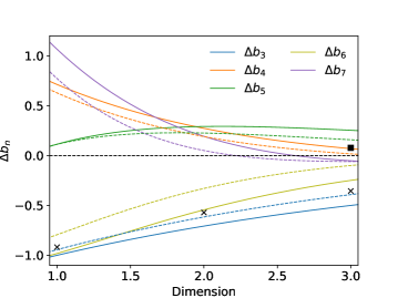
Figure 1: Interaction-induced change in virial coefficients $\Delta b_{3}$ – $\Delta b_{7}$ at $\Delta b_{2}=1/\sqrt{2}$ (which corresponds to the unitary limit in 3D), as a function of the spatial dimension $d$, in the LO- and NLO-SCLA (solid and dashed lines, respectively). The crosses represent $\Delta b_{3}$ as follows: Monte Carlo results in 1D from Ref. ShillDrut , diagrammatic results in 2D from Ref. Ngampruetikorn , and exact results in 3D Leyronas . The square shows the $\Delta b_{4}$ result of Ref. YanBlume .

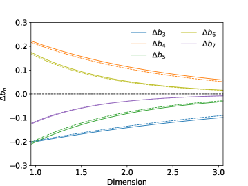
Figure 2: Interaction-induced change in virial coefficients $\Delta b_{3}$ – $\Delta b_{7}$ at $\Delta b_{2}=1/(5\sqrt{2})$ (which corresponds to a point on the BCS side of the resonance in 3D where the interaction-induced changes $\Delta b_{n}$ are of the same order at the noninteracting $b_{n}$), as a function of the spatial dimension $d$, in the LO- and NLO-SCLA (solid and dashed lines, respectively).

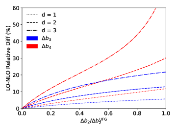
Figure 3: $|\Delta b_{3}^{\text{NLO}}/\Delta b_{3}^{\text{LO}}-1|$ (blue lines) and $|\Delta b_{4}^{\text{NLO}}/\Delta b_{4}^{\text{LO}}-1|$ (red lines) as percentages relative to the corresponding LO result, plotted as functions of $\Delta b_{2}/\Delta b_{2}^{\mathrm{UFG}}$ for $d=1,2,3$ (in dotted, dashed, and dashed-dotted, respectively).

IV.3 Application: pressure and Tan’s contact in 2D

In this section we apply our estimates of the virial coefficients to two simple thermodynamic observables: the pressure and Tan’s contact. For concreteness, we focus on the 2D attractive Fermi gas, but we emphasize that our results are explicit analytic functions of the dimension and can therefore be evaluated for arbitrary $d$.

To access the pressure, we combine the calculated virial coefficients according to

$$-\beta\Delta\Omega=Q_{1}\sum_{m=1}^{\infty}\Delta b_{m}z^{m},$$ (46)

where $\Delta\Omega=-\Delta PV$ is the change in the pressure $P$ due to interaction effects. From this equation, it is straightforward to determine the density change $\Delta n$ and the compressibility change $\Delta\chi$ by differentiation with respect to $z$. In Fig. 4 we show the pressure, in units of its noninteracting counterpart $P_{0}$, as a function of $\beta\mu=\ln z$, for the 2D Fermi gas with attractive interactions, for the LO- (top) and NLO-SCLA (bottom). The results at NLO show somewhat improved agreement with previous results at all couplings studied when considering the full expressions that include $\Delta b_{7}$.

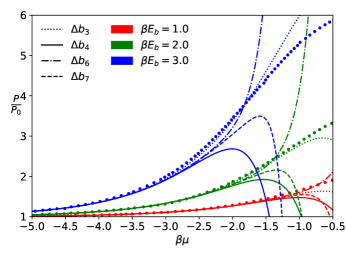
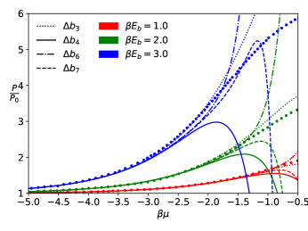
Figure 4: Pressure $P$ of the 2D attractively interacting Fermi gas, in units of the noninteracting pressure $P_{0}$, both as functions of $\beta\mu$. The lines show our LO-SCLA (top) and NLO-SCLA (bottom) results at various orders in the virial expansion. The dots correspond to the quantum Monte Carlo calculations of Ref. AndersonDrut . The colors indicate the value of the coupling: from top to bottom the sets of curves correspond to $\beta\epsilon_{B}=3.0$ (blue), $2.0$ (green), and $1.0$ (red).

Within the context of the LO- and NLO-SCLA results for $\Delta b_{n}$, Fig. 4 provides an indication of the range of validity of the virial expansion. In those plots, the large oscillations observed as $\beta\mu$ is increased show that the radius of convergence $r$ of the virial expansion, as a function of $z$, is notably reduced as the coupling is increased. For $\beta\epsilon_{B}=1$, we have $r\simeq\exp(-1.25)$, whereas for $\beta\epsilon_{B}=3$, we have $r\simeq\exp(-2.75)$. Such an effect is expected but, to understand to what extent that reduction is due to the LO approximation, higher orders in the approximation must be investigated.

To obtain Tan’s contact Tan , we differentiate with respect to the coupling $\lambda$ (i.e. we use the so-called adiabatic relation). In this case, since we use $\Delta b_{2}$ as our physical dimensionless coupling (or as a proxy to scattering parameters or binding energies), we simply differentiate $\Delta\Omega$ with respect to that parameter and obtain the dimensionless form

$$\frac{\Delta\mathcal{C}}{Q_{1}}=\sum_{m=1}^{\infty}\frac{\partial\Delta b_{m}}{\partial\Delta b_{2}}z^{m}.$$ (47)

To connect the above expression to the conventional form of Tan’s contact we only need the overall factor $\partial b_{2}/\partial\lambda$, where $\lambda$ is the coupling. Such a factor contains only two-body physics and can therefore be calculated explicitly using the well-known Beth-Uhlenbeck formula BU . In Fig. 5 we show our results for ${\Delta\mathcal{C}}/{Q_{1}}$ as a function of $\beta\mu=\ln z$, for the 2D Fermi gas with attractive interactions. Although somewhat more difficult to visualize, we glean from this figure that the virial expansion breaks down at lower values of $\beta\mu$ at stronger couplings.

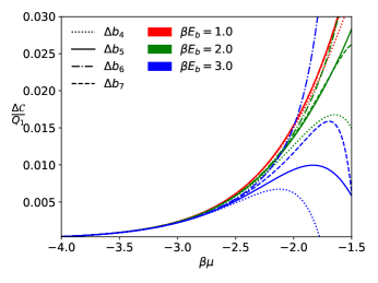
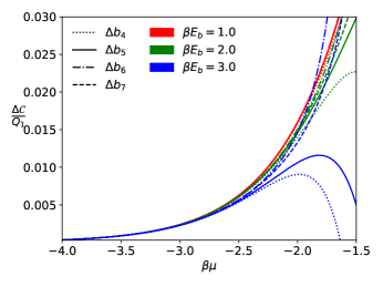
Figure 5: Many-body contribution to Tan’s contact as a function of $\beta\mu$ in the virial expansion, per Eq. (47) The lines show our LO-SCLA (top) and NLO-SCLA (bottom) results at various orders in the virial expansion. The colors indicate the value of the coupling: $\beta\epsilon_{B}=3.0$ (blue), $2.0$ (green), and $1.0$ (red).

V Summary and Conclusions

In this work, we calculated the virial coefficients of spin-$1/2$ fermions in the LO-SCLA, up to $\Delta b_{7}$. We have presented analytic results on the lattice and, much more succinctly, in the continuum limit, where they feature an explicit analytic dependence on the number of spatial dimensions $d$.

As a renormalization prescription, we fixed the bare constant $C$ by using the fact that $\Delta b_{2}$ is in many cases known analytically through the Beth-Uhlenbeck formula BU (see e.g. Refs. EoS1D ; virial2D ; virial2D2 ; PhysRevA.89.013614 ; Daza2D ; LeeSchaeferPRC1 ). That choice allowed us to express our results in powers of $\Delta b_{2}$ and to perform cross-dimensional comparisons by varying $d$ at fixed $\Delta b_{2}$. In turn, that comparison shows that the SCLA behaves qualitatively as expected. Notably, the agreement for $\Delta b_{3}$ improves across dimensions when going from LO to NLO, but it appears to deteriorate for $\Delta b_{4}$ at unitarity. To better understand that feature, we showed results at weaker couplings, which show much better convergence (i.e. much smaller changes) when going from LO to NLO for all the $\Delta b_{n}$ studied. These results are encouraging towards exploring higher orders in the SCLA, which will be carried out elsewhere HouDrut .

The fact that we have used the continuum limit of momentum sums in our final answers, together with the continuum $\Delta b_{2}$ result to fix the coupling, does not eliminate all the lattice artifacts. Indeed, implicit in our derivations is the spatial lattice spacing $\ell$, with which the coupling runs and which induces finite-range effects. To avoid such effects, future studies should use improved actions (see e.g. DrutNicholson ; Drut ).

Finally, it should be stressed that the applicability of the SCLA goes beyond the approximation of virial coefficients. In the form implemented here, it can be used to access the thermodynamics of finite systems. For those, the SCLA simply represents the non-perturbative analytic evaluation of a finite-temperature lattice calculation which would not be possible due to the sign problem, and which is carried out in a coarse temporal lattice.

Appendix A Matrices

In this section we provide the detailed form of the matrices that appear in the evaluation of the functions in Tables 1, 2, and 3. To that end, it is useful to define the following notation:

$$M_{0}=\begin{pmatrix}0&1&-1\\ 1&0&-1\\ -1&-1&0\\ \end{pmatrix},\ \ \ \ \ \text{diag}(a,b,c)=\begin{pmatrix}a&0&0\\ 0&b&0\\ 0&0&c\\ \end{pmatrix}.$$ (48)

Using the above, we have

$$M_{4} = \text{diag}(2,2,2)+M_{0}$$ (49)

$$M_{5} = \text{diag}(3,2,2)+M_{0}$$ (50)

$$M_{6a} = \text{diag}(4,4,4)+3M_{0}$$ (51)

$$M_{6b} = \text{diag}(3,2,3)+M_{0}$$ (52)

$$M_{6c} = \text{diag}(4,3,3)+2M_{0}$$ (53)

$$M^{(2)}_{7a} = \text{diag}(5,4,4)+3M_{0}$$ (54)

$$M^{(2)}_{7b} = \text{diag}(5,2,2)+M_{0}$$ (55)

$$M^{(2)}_{7c} = \text{diag}(4,4,3)+2M_{0}$$ (56)

$$M^{(3)}_{7a} = \text{diag}(2,3,2)+M_{0}$$ (57)

$$M^{(3)}_{7b} = \text{diag}(3,3,2)+M_{0}$$ (58)

$$M^{(3)}_{7c} = \text{diag}(4,4,4)+3M_{0}$$ (59)

$$N_{1}=\begin{pmatrix}3&2&-1&-1\\ 2&3&-1&-1\\ -1&-1&2&0\\ -1&-1&0&2\\ \end{pmatrix}$$ (60)

$$N_{2}=\begin{pmatrix}4&2&-1&-1\\ 2&3&-1&-1\\ -1&-1&2&0\\ -1&-1&0&2\\ \end{pmatrix}.$$ (61)

Appendix B High-order virial expansion formulas

For completeness, we provide here some of the formulas which we omitted in the main text for the sake of brevity and clarity. These are model independent, except as noted below. The complete expressions for $b_{5}$, $b_{6}$, and $b_{7}$ in terms of the corresponding canonical partition functions and prior virial coefficients can be written as

$$Q_{1}b_{5} = Q_{5}-(b_{4}+b_{2}b_{3})Q_{1}^{2}-\left(b_{2}^{2}+b_{3}\right)\frac{Q_{1}^{3}}{2}$$ (62)

$$-b_{2}\frac{Q_{1}^{4}}{3!}-\frac{Q_{1}^{5}}{5!},$$

$$Q_{1}b_{6} = Q_{6}-\left(b_{5}+\frac{b_{3}^{2}}{2}+b_{2}b_{4}\right)Q_{1}^{2}$$ (63)

$$-\left(\frac{b_{2}^{3}}{6}+\frac{b_{4}}{2}+b_{3}b_{2}\right)Q_{1}^{3}$$

$$-\left(\frac{b_{2}^{2}}{2}+\frac{b_{3}}{3}\right)\frac{Q_{1}^{4}}{2!}-b_{2}\frac{Q_{1}^{5}}{4!}-\frac{Q_{1}^{6}}{6!},$$

$$Q_{1}b_{7} = Q_{7}-(b_{6}+b_{2}b_{5}+b_{3}b_{4})Q_{1}^{2}$$ (64)

$$-\left(\frac{b_{3}^{2}}{2}+\frac{b_{5}}{2}+b_{2}b_{4}+\frac{b_{3}b_{2}^{2}}{2}\right)Q_{1}^{3}$$

$$-\left(\frac{b_{2}^{3}}{6}+\frac{b_{4}}{6}+\frac{b_{3}b_{2}}{2}\right)Q_{1}^{4}$$

$$-\left(b_{2}^{2}+\frac{b_{3}}{2}\right)\frac{Q_{1}^{5}}{12}-b_{2}\frac{Q_{1}^{6}}{5!}-\frac{Q_{1}^{7}}{7!},$$

whereas the change in the above due to interactions (assuming here two-body interactions) are given by

$$Q_{1}\Delta b_{5} = \Delta Q_{5}-\Delta(b_{4}+b_{2}b_{3})Q_{1}^{2}-\frac{1}{2}\Delta\left(b_{2}^{2}+b_{3}\right)Q_{1}^{3}-\frac{\Delta b_{2}}{3!}Q_{1}^{4},$$ (65)

$$Q_{1}\Delta b_{6} = \Delta Q_{6}-\Delta\left(b_{5}+\frac{b_{3}^{2}}{2}+b_{2}b_{4}\right)Q_{1}^{2}-\Delta\left(\frac{b_{2}^{3}}{6}+\frac{b_{4}}{2}+b_{3}b_{2}\right)Q_{1}^{3}-\Delta\left(\frac{b_{2}^{2}}{4}+\frac{b_{3}}{6}\right)Q_{1}^{4}-\frac{\Delta b_{2}}{4!}Q_{1}^{5},$$ (66)

$$Q_{1}\Delta b_{7} = \Delta Q_{7}-\Delta(b_{6}+b_{2}b_{5}+b_{3}b_{4})Q_{1}^{2}-\Delta\left(\frac{b_{3}^{2}}{2}+\frac{b_{5}}{2}+b_{2}b_{4}+\frac{b_{3}b_{2}^{2}}{2}\right)Q_{1}^{3}-\Delta\left(\frac{b_{2}^{3}}{6}+\frac{b_{4}}{6}+\frac{b_{3}b_{2}}{2}\right)Q_{1}^{4}$$ (68)

$$-\Delta\left(\frac{b_{2}^{2}}{12}+\frac{b_{3}}{24}\right)Q_{1}^{5}-\frac{\Delta b_{2}}{5!}Q_{1}^{6}.$$

To use these, it is useful to have the following:

$$\Delta(b_{n})^{2} = \Delta(b_{n}^{2})+2b_{n}^{(0)}\Delta b_{n},$$ (69)

$$\Delta(b_{n})^{3} = \Delta(b_{n}^{3})+3b_{n}^{(0)}\Delta(b_{n}^{2})+3(b_{n}^{(0)})^{2}\Delta b_{n},$$ (70)

$$\Delta(b_{n}b_{m}) = \Delta b_{n}\Delta b_{m}+b_{n}^{(0)}\Delta b_{m}+b_{m}^{(0)}\Delta b_{n},$$ (71)

$$\Delta(b_{n}b_{m}^{2}) = \Delta b_{n}(\Delta b_{m})^{2}+b_{n}^{(0)}(\Delta b_{m})^{2}+2b_{m}^{(0)}\Delta b_{n}\Delta b_{m}$$ (72)

$$\!\!\!\!\!\!\!\!+2b_{n}^{(0)}b_{m}^{(0)}\Delta b_{m}+(b_{m}^{(0)})^{2}\Delta b_{n}.$$

References

• (1) C. R. Shill, J. E. Drut, Virial coefficients of 1D and 2D Fermi gases by stochastic methods and a semiclassical lattice approximation, Phys. Rev. A 98, 053615 (2018).
• (2) X.-J. Liu, Virial expansion for a strongly correlated Fermi system and its application to ultracold atomic Fermi gases, Phys. Rep. 524, 37 (2013).
• (3) Supplemental Materials: Python code for the evaluation of $\Delta b_{n}$ for $n=1,...,7$ in $d=1,2,3$, with ancillary files for renormalization by calculating $\Delta b_{2}$ in each dimension as a function of the scattering length.
• (4) V. Ngampruetikorn, M. M. Parish, and J. Levinsen, High-temperature limit of the resonant Fermi gas, Phys. Rev. A 91, 013606 (2015).
• (5) X.-J. Liu, H. Hu, and P. D. Drummond, Exact few-body results for strongly correlated quantum gases in two dimensions, Phys. Rev. B 82, 054524 (2010).
• (6) X. Leyronas, Virial expansion with Feynman diagrams, Phys. Rev. A 84, 053633 (2011).
• (7) X.-J. Liu, H. Hu, and P. D. Drummond, Virial expansion for a strongly correlated Fermi gas, Phys. Rev. Lett. 102, 160401 (2009).
• (8) D. B. Kaplan, S. Sun, A new field theoretic method for the virial expansion, Phys. Rev. Lett. 107, 030601 (2011).
• (9) Y. Yan, D. Blume, Path integral Monte Carlo determination of the fourth-order virial coefficient for unitary two-component Fermi gas with zero-range interactions, Phys. Rev. Lett. 116, 230401 (2016).
• (10) D. Rakshit, K. M. Daily, and D. Blume, Natural and unnatural parity states of small trapped equal-mass two-component Fermi gases at unitarity and fourth-order virial coefficient, Phys. Rev. A 85, 033634 (2012).
• (11) V. Ngampruetikorn, M. M. Parish, J. Levinsen, High-temperature limit of the resonant Fermi gas, Phys. Rev. A 91, 013606 (2015).
• (12) E. R. Anderson, J. E. Drut, Pressure, compressibility, and contact of the two-dimensional attractive Fermi gas, Phys. Rev. Lett. 115, 115301 (2015).
• (13) S. Tan, Ann. Phys. 323, 2952 (2008); ibid. 323, 2971 (2008); ibid. 323, 2987 (2008); S. Zhang, A. J. Leggett, Phys. Rev. A 77, 033614 (2008); F. Werner, ibid. 78, 025601 (2008); E. Braaten, L. Platter, Phys. Rev. Lett. 100, 205301 (2008); E. Braaten, D. Kang, L. Platter, ibid. 104, 223004 (2010).
• (14) E. Beth and G. E. Uhlenbeck, The quantum theory of the non-ideal gas. II. Behaviour at low temperatures, Physica (Utrecht) 4, 915 (1937).
• (15) M. D. Hoffman, P. D. Javernick, A. C. Loheac, W. J. Porter, E. R. Anderson, and J. E. Drut, Universality in one-dimensional fermions at finite temperature: Density, compressibility, and contact, Phys. Rev. A 91, 033618 (2015).
• (16) C. Chaffin and T. Schäfer, Scale breaking and fluid dynamics in a dilute two-dimensional Fermi gas, Phys. Rev. A 88, 043636 (2013).
• (17) V. Ngampruetikorn, J. Levinsen, and M. M. Parish, Pair correlations in the two-dimensional Fermi gas, Phys. Rev. Lett. 111, 265301 (2013).
• (18) M. Barth and J. Hofmann, Pairing effects in the nondegenerate limit of the two-dimensional Fermi gas, Phys. Rev. A. 89, 013614 (2014).
• (19) W. S. Daza, J. E. Drut, C. L. Lin, and C. R. Ordóñez, Virial expansion for the Tan contact and Beth-Uhlenbeck formula from two-dimensional SO(2,1) anomalies Phys. Rev. A 97, 033630 (2018).
• (20) D. Lee and T. Schäfer, Cold dilute neutron matter on the lattice. I. Lattice virial coefficients and large scattering lengths Phys. Rev. C 73, 015201 (2006).
• (21) Y. Hou and J. E. Drut, In preparation.
• (22) J. E. Drut and A. N. Nicholson, Lattice methods for strongly interacting many-body systems, J. Phys. G: Nucl. Part. Phys. 40, 043101 (2013).
• (23) J. E. Drut, Improved lattice operators for non-relativistic fermions, Phys. Rev. A 86, 013604 (2012).