Abstract

We consider a hybrid method to simulate the return time to the initial state in a critical–case birth–death process. The expected value of this return time is infinite, but its distribution asymptotically follows a power–law. Hence, the simulation approach is to directly simulate the process, unless the simulated time exceeds some threshold and if it does, draw the return time from the tail of the power law.

Keywords : birth–death process, infinite mean, phylogenetic tree, power–law distribution, return time

1 Introduction: a model for phylogenetic trees

Birth–and–death processes are frequently used today to model various branching phenomena, e.g. phylogenetic trees. Empirically observed (or rather estimated from e.g. genetic data) phylogenies can exhibit multiple patterns, e.g. many co–occurring species or only a dominating one at a given time instance. The HIV phylogeny is an example of the former, while the influenza phylogeny of the latter. During a given season there is one main flu virus going around, but it may change between seasons.

In [6] a very similar model that (depending on the choice of a parameter $\lambda$) can generate both patterns was proposed. They model the amount of types alive at a given time instance as follows. Assume that at time $t$ there are $N(t)>0$ types present. Then, at time $t$ the birth rate of the types is $\lambda N(t)$ and the death rate is $N(t)$. Each type has at birth, independently of the other types, a fitness value attached to it. If a death event occurs, the type with the lowest fitness goes extinct. The type with the largest value of the fitness is called the dominating type. As only the ranking of the types’ fitness is relevant the distribution of the fitness values does not matter.

The main result of [6] is the characterization of the lifetime of the dominating type.

Theorem 1.1 (Thm. $1$ in [6])

Take $\delta\in(0,1)$. If $\lambda\leq 1$, then

$$\lim\limits_{t\to\infty}P(dominating~{}types~{}at~{}\delta t~{}and~{}t~{}are~{}the~{}same)=\delta,$$

while if $\lambda>1$, then this limit is $0$.

Obviously, if $\lambda\leq 1$, then a given (maximal) type can persist (like influenza) but when $\lambda>1$, then there will be frequent switching between dominating types (like HIV—we cannot observe which strain dominates). The key object in the proof of Thm. 1.1 are the random times of hitting state $1$, conditional on having started in state $2$, we denote this random variable by $H$. Then, the waiting time for returning from state $1$ to state $1$ can be represented as $X+H$, where $X\sim\exp(\lambda)$. Naturally state $0$ is an absorbing state of the process. However, we do not worry about this, as it is assumed that if there is only one type, then it cannot die [6], i.e. $0$ will never be reached and the process starts anew in $1$.

Let $F(t)$ denote the cumulative distribution function (cdf) of $H$, i.e. $F(t)=P(H\leq t)$. Here we will focus on the critical case $(\lambda=1)$. In [6] it was claimed that in this regime $F(t)=t/(t+1)$ (proof of Lemma $3$ therein). However, in [1] it was shown that this statement is not true (cf. Eqs. $3.3$ and $3.4$ therein) however the right asymptotic behaviour of $F(t)$ is known (cf Eq. $3.2$ therein),

$$\lim\limits_{t\to\infty}t(1-F(t))=1.$$ (1)

To be able to work with the law of $H$ we introduce the following definition.

Definition 1.1

We say that a random variable $Y$ follows a power–law probability distribution with parameter $\gamma>0$, if it has support on $(y_{\min},\infty)$, $y_{\min}\geq 0$, and its law asymptotically satisfies

$$P(Y>y)\sim Cy^{-\gamma},~{}~{}~{}~{}~{}\mathrm{i.e.}~{}\lim\limits_{y\to\infty}y^{\gamma}P(Y>y)=C,$$

for some constant $C$.

Moments of order $m\geq\gamma$ are infinite.

Lemma 1.2

$H$ is a positive random variable that follows a power law distribution with $C=1$, $\gamma=1$ and

$$\operatorname{E}\left[H\right]=\infty.$$

Proof $H$ is positive by construction as a random sum of exponential random variables. From Eq. (1) we know that $\lim\limits_{y\to\infty}yP(H>y)=1$, corresponding to a power law distribution with $C=1$, $\gamma=1$ in Defn. 1.1. Hence, for $m\geq 1$ it holds directly that

$$\operatorname{E}\left[H^{m}\right]=\int\limits_{0}^{\infty}P(H^{m}>y)\mathrm{d}y=\infty.$$

$\Box$

Remark 1.3

It is worth noting that the infinite mean can be derived directly from the model formulation also. Denote by $H_{j}$ the time to reach state $1$ from state $j$ and $h_{j}=\operatorname{E}\left[H_{j}\right]$. Then, $H=H_{2}$ and define $H_{1}=0$. Notice that by the memoryless property of the process we can see that $h_{j}$ is a non–decreasing sequence, to get from state $j$ to state $1$ one has to return to state $j-1$.

By model construction we have $h_{2}=1/4+h_{3}/2$ and

$$h_{3}=\frac{1}{6}+\frac{1}{2}h_{2}+\frac{1}{2}h_{4},$$

giving

$$h_{2}=h_{3}+(h_{3}-h_{4})-\frac{1}{3}.$$

In the same way one will have for all $j\geq 3$

$$h_{j}-h_{j+1}=h_{j+1}+(h_{j+1}-h_{j+2})-\frac{1}{j+1}$$

resulting in for every $N\geq 3$

$$h_{2}=h_{3}+(h_{N}-h_{N+1})-\sum\limits_{i=3}^{N}\frac{1}{i}.$$

As obviously $h_{2}\geq 0$, one needs for every $N\geq 3$

$$h_{3}\geq h_{N+1}-h_{N}+\sum\limits_{i=3}^{N}\frac{1}{i}\geq\sum\limits_{i=3}^{N}\frac{1}{i}$$

implying that $h_{3}=\infty$. As $h_{2}=1/4+h_{3}/2$, then immediately $h_{2}=\infty$.

2 Simulation algorithm

Very often an important component of studying stochastic models is the possibility to simulate them. This is in order to illustrate the model, gather intuition for its properties, back–up (i.e. check for errors) analytical results and to design Monte Carlo based estimation or testing procedures. A Markov process as described in Section 1 is in principle trivial to simulate using the Gillespie algorithm [5]. Let $N_{n}$ be the embedded Markov Chain, i.e. $N_{n}=N(t_{n})$, where $t_{n}$ is the time of the $n$–th birth or death event. If the process is in state $N_{n}=i$ at step $n$, then one draws an exponential with rate $(i+i\lambda)$ waiting time and $N_{n+1}=i+\xi$, where $P(\xi=1)=\lambda i/(i+\lambda i)$ and $P(\xi=-1)=i/(i+\lambda i)$. However, in the critical case $\lambda=1$, as we showed that $\operatorname{E}\left[H\right]=\infty$, we cannot expect to reliably sample the full distribution of the chain’s trajectory. The tails will be significantly undersampled. In the simplest case if we want to plot an estimate of $H$’s density (e.g. a histogram), then we can expect its right tail to be significantly (in the colloquial sense) too light.

Unfortunately, only the asymptotic behaviour of $H$’s survival function, $1-F(t)$, is known. Therefore, if we were to draw from this form, we should firstly expect the initial part of the histogram to be badly found. Furthermore, as the constant $C=1$ in Eq. 1, then we know that the cumulative distribution function related to $F(t)$, $1-1/t$, has non–zero support on $[1,\infty)$. Obviously $H$ can take values also in $(0,1)$, so the above does not suffice.

Therefore, in this work we propose a hybrid algorithm that combines both approaches. Intuitively the left side of the histogram is simulated directly, while the right side is drawn from the asymptotic. We have as our aim a proof of concept study—to see if reasonable results can be obtained, leaving improvements of the algorithm and its analytical properties for further work.

Let $p$ be the proportion of simulations that we do not want to simulate directly but draw from the asymptotic. Define $T_{\min}$ as the value for which

$$p=P(H>T_{\min})=1-F(T_{\min})\approx T_{\min}^{-1}.$$

This gives $T_{\min}=p^{-1}$. We will use $p^{-1}$ and $T_{\min}$ interchangeably depending on the focus—the tail probability or the threshold value.

Algorithm 1 Simulating return time to state $1$

1:Initialize $p$, $T_{\min}=p^{-1}$, $N=2$, $H=0$

2:while $H\leq T_{\min}$ and $N\neq 1$ do

3:     draw $u\sim\exp(2N)$

4:     $H=H+u$

5:     if  $H\leq T_{\min}$ then

6:         $N=N+\xi$ $\triangleright$ $P(\xi=1)=P(\xi=-1)=\frac{1}{2}$

7:     end if

8:end while

9:if $H>T_{\min}$ or $N\neq 1$ then

10:     $H=$poweRlaw::rplcon(1,xmin=$T_{\min}$,alpha=2) $\triangleright$ See Section 2

11:end if

12:draw $t\sim\exp(1)$

13:return $(H,H+t)$ $\triangleright$ $H+t$ is return time from $2$ to $1$

The hybrid simulation approach is described in Alg. 1. Until the waiting time does not exceed a certain threshold the simulations proceeds directly according to the model’s description. The threshold simulation is chosen so that (approximately, according to the limit distribution) with probability $1-p$ it will not be exceeded. If the threshold is exceeded, then $H$ is drawn from a law corresponding to the survival function’s asymptotic behaviour. There is a trade–off in the choice of $p$. If we choose a small $p$, i.e. a threshold far in the right tail, then with high probability we will have an exact simulation algorithm. However, on the other hand the running time may be large. In contrast, taking a larger $p$ will reduce the running time, however, more samples will not be drawn exactly but from the asymptotic, and our final simulated value’s distribution could be further away from its true law. Obviously, $p\in(0,1)$ by it being a probability and the previously discussed properties of the asymptotics of the survival function, i.e. $C=1$.

In order to draw from the law corresponding to the asymptotic behaviour of the right tail of the survival function, we use the powerRlaw [4] R [7] package. The poweRlaw::rplcon(1,$T_{\min}$,$\alpha$) draws a single value from a power law supported on $(T_{\min},\infty)$ with density and cumulative distribution functions (Eq. $(1)$, $(4)$, [4]) equalling

$$p(t)=\frac{\alpha-1}{T_{\min}}\left(\frac{t}{T_{\min}}\right)^{-\alpha},~{}~{}~{}P(T\leq t)=1-\left(\frac{t}{T_{\min}}\right)^{-\alpha+1}$$ (2)

for $\alpha>1$ and $T_{\min}>0$. Note the correspondance between Defn. 1.1 and Eq. (2), $\gamma=\alpha-1$.

In our situation we have $1-F(t)\sim t^{-1}$. Hence, we can take the power law corresponding to the limit as the cdf $F_{\infty}(t)=(1-t^{-1})\mathbf{1}_{t>1}$, with density equalling $f_{\infty}(t)=t^{-2}$ on $(1,\infty)$. This implies taking $\alpha=2$ when calling poweRlaw::rplcon(). As we have defined a threshold of $p^{-1}$, we need to include it also when drawing the value, i.e. we do not want to have empty draws of too small values. Setting, then $T_{\min}=p^{-1}$, tells poweRlaw::rplcon() that our law is concentrated on $(T_{\min},\infty)$. Notice that we are working with the conditional random variable $H$, given that $H>T_{\min}$. Its conditional cdf will equal $p^{-1}(F_{\infty}(t)-F_{\infty}(T_{\min}))\mathbf{1}_{t>T_{\min}}$, with associated density $p^{-1}t^{-2}\mathbf{1}_{t>T_{\min}}$, but this equals $p(t)=(1/p)^{-1}(xp^{-1})^{-2}\mathbf{1}_{t>T_{\min}}$. The function poweRlaw::rplcon() draws a value using the inverse cdf method. Let $U\sim\mathrm{Unif}[0,1]$, and then $T$ from poweRlaw::rplcon() is given by

$$T=T_{\min}(1-U)^{-1/(\alpha-1)}.$$

As we do not know from what value the tail asymptotics are a good approximation we cannot a priori be sure whether the threshold will be exceeded with probability $p$, nor if after $p^{-1}$ the sampling of $H$ from the limit will be accurate. These important properties will be checked empirically in the simulation study in Section 3.

3 Simulation setup and results

The simulation study presented here has a number of aims, to illustrate the distribution of waiting times $H$ as simulated exactly and via Alg. 1. Secondly, to study whether Alg. 1 is a sensible approach to to simulating this random time. All simulations were done in R version $3.4.2$ [7] running on an openSUSE $42.3$ ($x86$_$64$) box with a $3.50$GHz Intel^® Xeon^® CPU.

Simulating the Markov process directly (and then extracting $H$) is a straightforward procedure. However, as $\operatorname{E}\left[H\right]=\infty$, we introduce a cutoff, if the number of steps exceeds a given number, here $10^{8}$, we end the simulation and mark that the process did not return to state $1$. Out of the $10^{7}$ repeats, $767$ reached the maximum allowed number of steps, $10^{8}$. In order to see how well Alg. 1 is corresponding to the true distribution of $H$, we re–run it for two values of $p$, $p_{1}=0.0001$ and $p_{2}=0.0005$. Then, we compare the logarithms of the survival functions, of both simulations and furthermore on the interval $(p_{2}^{-1},p_{1}^{-1})$, Fig. 1. The first sample, with threshold $p_{1}^{-1}$, can be thought of as the “true one” on this interval, as $H$ was simulated exactly—directly from the model’s definition. We present the logarithm of the survival function as otherwise nothing would be visible from the plot, due to the heavy tail. The power–law property of the tail can be clearly seen in the left panel of Fig. 1. In fact, if one regress $\log(y)$ on $\log(x)$ one will obtain a slope estimate of $-1.010$ $(p_{1})$ or $-0.9375$ $(p_{2})$. This is in agreement with our result that $1-F(t)\sim t^{-1}$. Out of the $10^{7}$ simulations only $992$ had $H>p_{1}^{-1}=10000$ in the case of the $p_{1}$ simulation and $4992$ instances had $H>p_{2}^{-1}=2000$ in the case of the $p_{2}$ simulation. We can see that these correspond nearly exactly to the desired proportion of exceeding the cutoff, i.e. $992/10^{7}=0.0000992\approx p_{1}=0.0001$ and $4992/10^{7}=0.0004992\approx p_{2}=0.0005$.

4 Discussion

The results presented here indicate that a hybrid approach for simulating the waiting time to return to state $1$ in the considered birth–death model is a promising one. From Figs. 2 and 3 it is evident that the direct approach cannot capture the heavy tail. When, the simulation was stopped due to exceeding a time/step limit these figures show that the process was usually far on the right and not approaching $1$.

For our considered hybrid procedure to be effective one needs to appropriately choose the threshold $p^{-1}$. If it is too small, then the return time might not yet be in the asymptotic regime. If it is too large, then the running time can be too long. In our case $10^{7}$ repeats with $p_{2}=0.0005$ took about $68.5$ hours while for $p_{1}=0.0001$ it took about $15.6$ days. Definitely $p_{1}^{-1}$ is too large for a threshold, while $p_{2}^{-1}$ will be acceptable given that the required sample size is smaller. Most importantly, the comparison between $p_{1}$’s and $p_{2}$’s results, in Fig. 1, showed that with $p_{2}=0.0005$ the hybrid approach yields samples that do not seem to be distinguishable from the true law. This is as on the interval $(p_{2}^{-1},p_{1}^{-1})$ the $p_{1}$ simulation is exact.

Our study here points to three possible, exciting future directions of development. Firstly, to identify an optimal value for $p$. Secondly, to develop a better simulation approach so that when $H$ exceeds $p$ and the draw “has to be made from the tail”, the simulated path does not need to be discarded, i.e. to characterize the law of the return time from an arbitrary state $m$ to state $1$. And lastly the study of $1-F(t)-t^{-1}$ i.e. how does the survival function deviate from its asymptotic behaviour.

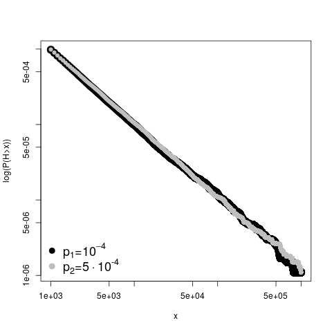
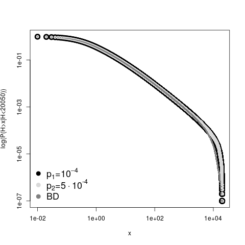
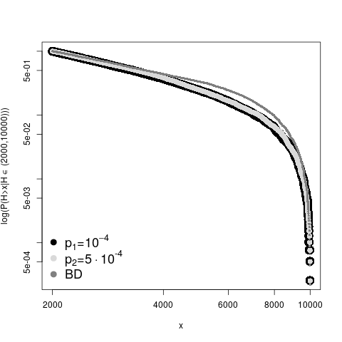
Figure 1: Logarithms of survival functions created using R’s ecdf() function to estimate the cdf. Left: comparison of the survival functions for $p_{1}$ and $p_{2}$, centre: comparison of the survival functions for $p_{1}$, $p_{2}$ and the “direct” simulation (on the interval $(0,20050)$, where the “direct” simulation produced values), right: comparison of the survival functions for $p_{1}$, $p_{2}$ and the “direct” simulation on the interval $(p_{2}^{-1},p_{1}^{-1})$. For readability the right plot starts from $1000$. In the centre plot the “direct” simulation is conditional on the number of steps being lesser than $10^{8}$, so this survival function is a conditional one. The Kolmogorov–Smirnov test, ks.test() function, was used to check for differences between the empirical distributions. All p–values exceeded $0.277$, except for the (right plot) comparison on the interval $(p_{2}^{-1},p_{1}^{-1})$, between “direct” and $p_{1}$ simulation $(5.551\cdot 10^{-16})$ and “direct” and $p_{2}$ simulation $(2.331\cdot 10^{-15})$. Here, the p–value when testing the $p_{1}$ versus the $p_{2}$ simulation equalled $0.277$. The $x$–axes are on the log scale.

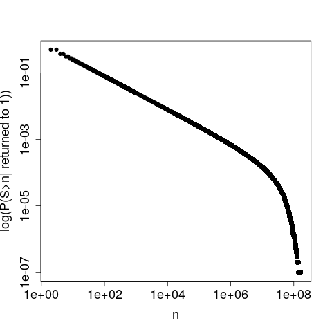
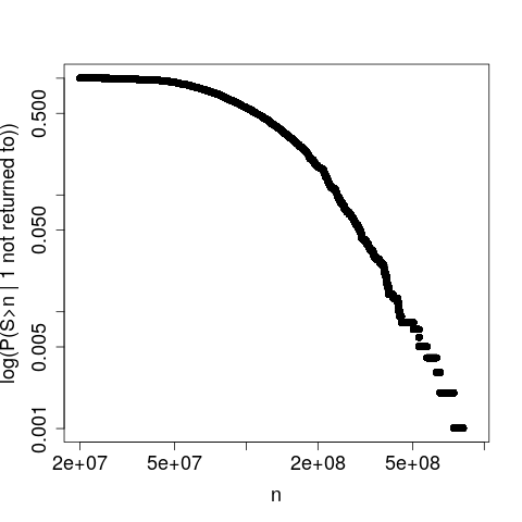
Figure 2: Comparison of the number of steps in the $p_{1}$ simulation, using the logarithm of the survival function. Left: when state $1$ was returned to, right: state $1$ was not returned to, i.e. $H>p_{1}^{-1}=10000$.

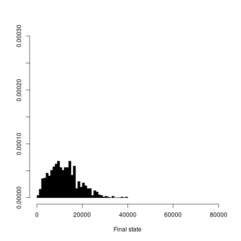
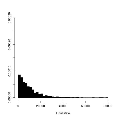
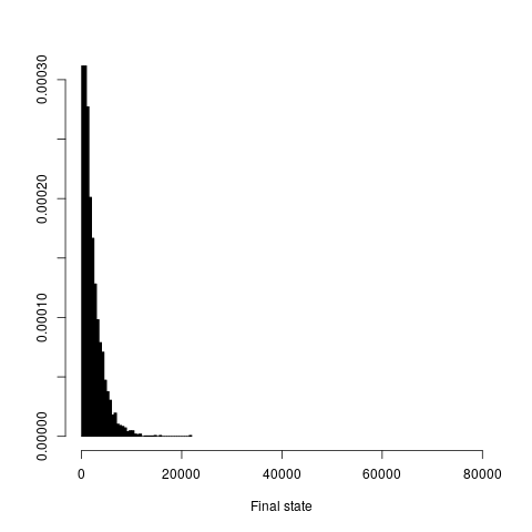
Figure 3: The final state reached when state $1$ was not returned to in the direct simulation. Left: “direct” simulation, centre: $p_{1}$ simulation, right: $p_{2}$ simulation. In the $p_{1}$ and $p_{2}$ simulations case, in these instances $H$ was obtained by sampling from poweRlaw::rplcon().

5 Acknowledgments

KB’s research is supported by the Swedish Research Council’s (Vetenskapsrådet) grant no. $2017$–$04951$. KB would like to thank the Editor and an anonymous Reviewer for careful reading of the manuscript and comments that greatly improved it. KB is grateful to Serik Sagitov for encouragement and suggestions to study general passage times between $m$ and $k$ in the considered here birth–death process.

Appendix: R code for simulating $H$ used in Section 3
 

⬇

f_dosim_Exact<-function(i,maxstep){

## Simulation of H directly from the Markov model

H<-0;waitT<-0;X<-2

b_1<-FALSE;n<-1

while((X!=1)&&(n<maxstep)){

n<-n+1

H<-H+rexp(1,rate=2*X) ## for lambda=1

X<-X+sample(c(-1,1),1) ## for lambda=1

}

if (X==1){b_1<-TRUE}

T1<-rexp(1)

c(T=T1+H,T1=T1,H=H,n=n,X=X,b_1=b_1)

}

⬇

f_dosim_PLcon<-function(i,p){

## simulation of H using the hybrid algorithm

Ttail<-1/p

T1<-rexp(1)

H<-0;X<-2

b_1<-FALSE;n<-1;sim_H<-0

while((X!=1)&&(sim_H<=Ttail)){

n<-n+1

moveT<-rexp(1,rate=2*X) ## for lambda=1

sim_H<-sim_H+moveT

if (sim_H<=Ttail){

H<-H+moveT

X<-X+sample(c(-1,1),1) ## for lambda=1

}

}

if ((X==1)&&(sim_H<=Ttail)){b_1<-TRUE}

else{

H<-poweRlaw::rplcon(1,xmin=Ttail,alpha=2)

}

c(T=H+T1,T1=T1,H=H,n=n,X=X,b_1=b_1,Ttail=Ttail,sim_H=sim_H,p=p)

}

References

- [1] K. Bartoszek, M. Krzemiński Critical case stochastic phylogenetic tree model via the Laplace transform, Demonstratio Mathematica 47, 474–481 (2014).
- [2] A. A. Borovkov, K. A. Borovkov, Asymptotic Analysis of Random Walks Heavy–Tailed Distributions, Cambridge University Press, 2008.
- [3] A. Clauset, C. R. Shalizi, M. E. J. Newman Power–law distributions in empirical data, SIAM Review 51, 661–703 (2009).
- [4] C. S. Gillespie Fitting heavy tailed distributions: the poweRlaw package, J. Stat. Softw. 64, 1–16 (2015).
- [5] D. T. Gillespie Exact Stochastic Simulation of Coupled Chemical Reactions, J. Phys. Chem. 81, 2340–2361 (1977).
- [6] T. M. Liggett, R. B. Schinazi A stochastic model for phylogenetic trees, J. Appl. Probab. 46, 601–607 (2009).
- [7] R Core Team, R: A Language and Environment for Statistical Computing, R Foundation for Statistical Computing, Vienna; www.R-project.org, 2013.