On URANS Congruity with Time Averaging:
Analytical laws suggest improved models

Abstract

The standard $1-$equation model  of turbulence was first derived by Prandtl and has evolved to be a common method for practical flow simulations. Five fundamental laws that any URANS model should satisfy are

$$\begin{array}[c]{ccc}\text{{1.}}&\text{Time window:}&\begin{array}[c]{c}\tau\downarrow 0\text{ implies }v_{\text{{\small URANS}}}\rightarrow u_{\text{{\small NSE}}}\text{ \&}\\ \text{ }\tau\uparrow\text{implies }\nu_{T}\uparrow\end{array}\\ \text{{2.}}&\text{ \ }l(x)=0\ \text{at walls:}&l(x)\rightarrow 0\text{ as }x\rightarrow walls,\\ \text{{3.}}&\text{ Bounded energy:}&\sup_{t}\int\frac{1}{2}|v(x,t)|^{2}+k(x,t)dx<\infty\\ \text{{4.}}&\begin{array}[c]{c}\text{Statistical }\\ \text{equilibrium:}\end{array}&\lim\sup_{T\rightarrow\infty}\frac{1}{T}\int_{0}^{T}\varepsilon_{\text{model}}(t)dt=\mathcal{O}\left(\frac{U^{3}}{L}\right)\\ \text{{5.}}&\begin{array}[c]{c}\text{Backscatter}\\ \text{possible:}\end{array}&\text{(without negative viscosities)}\end{array}$$

This report proves that a kinematic specification of the model’s turbulence lengthscale by

$$l(x,t)=\sqrt{2}k^{1/2}(x,t)\tau\text{ },$$

where $\tau$ is the time filter window, results in a $1-$equation model satisfying Conditions 1,2,3,4 without model tweaks, adjustments or wall damping multipliers.

1 Introduction

URANS (unsteady Reynolds averaged Navier-Stokes) models of turbulence are derived commonly to produce a velocity, $v(x,t)\simeq\overline{u}(x,t)$, that approximates a finite time window average of the Navier-Stokes velocity $u(x,t)$

$$\overline{u}(x,t)=\frac{1}{\tau}\int_{t-\tau}^{t}u(x,t^{\prime})dt^{\prime}.$$ (1)

From this connection flows 5 fundamental conditions (below) that a coherent URANS model should satisfy and that few do. Herein we delineate these conditions and show that, for the standard $1-$equation model, a new kinematic turbulence length scale results in a simpler model satisfying 4 of the 5.

The first condition is a simple observation that the time window $\tau$ should influence the model, as $\tau\rightarrow 0$ the model should revert to the NSE (Navier-Stokes equations) and as $\tau$ increases, more time scales are filtered and thus the eddy viscosity should increase.

Condition 1: The filter window $\tau$ should appear as a model parameter. As $\tau\rightarrow 0$ the model reverts to the NSE. As $\tau$ increases, the model eddy viscosity $\nu_{T}(\cdot)$ increases.

We consider herein $1-$equation models of turbulence. These have deficiencies but nevertheless include models considered to have good predictive accuracy and low cost, e.g., Spalart [28] and Figure 2 p.8 in Xiao and Cinnella [37]. The standard $1-$equation model (from which all have evolved), introduced by Prandtl [25], is

$$v_{t}+v\cdot\nabla v-\nabla\cdot\left(\left[2\nu+\mu l\sqrt{k}\right]\nabla^{s}v\right)+\nabla p=f(x)\text{, }$$

$$\nabla\cdot v=0\text{, }$$ (2)

$$k_{t}+v\cdot\nabla k-\nabla\cdot\left(\left[\nu+\mu l\sqrt{k}\right]\nabla k\right)+\frac{1}{l}k\sqrt{k}=\mu l\sqrt{k}|\nabla^{s}v|^{2}\text{.}$$

Briefly, $p(x,t)$ is a pressure, $f(x)$ is a smooth, divergence free ($\nabla\cdot f=0$) body force, $\mu\simeq 0.55$ is a calibration parameter, $\nabla^{s}v=(\nabla v+\nabla^{T}v)/2$ is the deformation tensor, and $k(x,t)$ is the model approximation to the fluctuations’ kinetic energy distribution, $\frac{1}{2}|(u-\overline{u})(x,t)|^{2}$. The eddy viscosity coefficient

$$\nu_{T}(\cdot)=\mu l\sqrt{k}$$

(the Prandtl-Kolmogorov formula) is a dimensionally consistent expression of the observed increase of mixing with turbulence and of the physical idea of Saint-Venant [27] that this mixing increases with "the intensity of the whirling agitation", [7], p.235. The $k-$equation describes the turbulent kinetic energy evolution; see [5] p.99, Section 4.4, [6], [22] p.60, Section 5.3 or [24] p.369, Section 10.3, for a derivation. The model (2) holds in a flow domain $\Omega$ with initial conditions, $v(x,0)$ and $k(x,0)$, and (here $L-$periodic or no-slip) $v,k$ boundary conditions on the boundary $\partial\Omega$.

The parameter of interest herein is the turbulence length-scale $l=l(x)$, first postulated by Taylor in 1915 [30]. It varies from model to model, flow subregion to subregion (requiring fore knowledge of their locations, [28]) and must be specified by the user; see [35] for many examples of how $l(x)$ is chosen in various subregions. The simplest case is channel flow for which

$$l_{0}(x)=\min\{0.41y,0.082\mathcal{R}e^{-1/2}\}$$

where $y$ is the wall normal distance, Wilcox [35] Ch. 3, eqn. (3.99) p.76.

Model solutions are approximations to averages of velocities of the incompressible Navier-Stokes equations. Other fundamental physical properties of NSE solutions (inherited by averages) should also be preserved by the model. These properties include:

Condition 2: The turbulence length-scale $l(x)$ must $l(x)\rightarrow 0$ as $x\rightarrow walls$.

Condition 2 follows since the eddy viscosity term approximates the Reynolds stresses and

$$\mu l\sqrt{k}\nabla^{s}v\simeq u^{\prime}u^{\prime}\text{ which }\rightarrow 0\text{ at walls like }\mathcal{O}(\text{{wall-distance}}^{2}).$$

Specifications of $l(x)$ violating this are often observed to over-dissipate solutions (in many tests and now with mathematical support [23]).

Condition 3: (Finite kinetic energy) The model’s representation of the total kinetic energy in the fluid must be uniformly bounded in time:

$$\int_{\Omega}\frac{1}{2}|v(x,t)|^{2}+k(x,t)dx\leq Const.<\infty\text{ uniformly in time.}$$

The kinetic energy (per unit volume)$\frac{1}{|\Omega|}\int\frac{1}{2}|u|^{2}dx$, is distributed between means and fluctuations in the model as

$$\frac{1}{|\Omega|}\int_{\Omega}\frac{1}{2}|v(x,t)|^{2}+k(x,t)dx\simeq\frac{1}{|\Omega|}\int_{\Omega}\frac{1}{2}|u(x,t)|^{2}dx<\infty.$$

This property for the NSE represents the physical fact that bounded energy input does not grow to unbounded energy solutions.

Condition 4: (Time-averaged statistical equilibrium) The time average of the model’s total energy dissipation rate, $\varepsilon_{\text{model}}$ (4) below, should be at most the time average energy input rate:

$$\lim\sup_{T\rightarrow\infty}\frac{1}{T}\int_{0}^{T}\varepsilon_{\text{model}}(t)dt\leq Const.\frac{U^{3}}{L}\text{, uniformly in }\mathcal{R}e\text{.}$$

The most common failure model for turbulence models is over-dissipation. Condition 4 expresses aggregate non-over-dissipatiopn. The energy dissipation rate is a fundamental statistic of turbulence, e.g., [24], [31]. This balance is observed in physical experiments [13], [31] and has been proven for the NSE, [9], [8], [10].

The fifth condition is that the model allows an intermittent flow of energy from fluctuations back to means. This energy flow is important, e.g. [29], [32], less well understood and not addressed herein; for background see [15].

Condition 5: The model allows flow of energy from fluctuations back to means without negative eddy viscosities. This energy flow has space time average zero.

To develop Conditions 3 and 4, multiple the $v-$equation (2) by $v$ and integrate over $\Omega$. Add to this the $k-$ equation integrated over $\Omega$. After standard manipulations and cancellations of terms there follows the model’s global energy balance

$$\frac{d}{dt}\int_{\Omega}\frac{1}{2}|v(x,t)|^{2}+k(x,t)dx+\int_{\Omega}2\nu|\nabla^{s}v(x,t)|^{2}+\frac{1}{l(x)}k^{3/2}(x,t)dx$$ (3)

$$=\int_{\Omega}f(x)\cdot v(x,t)dx.$$

Thus, for the $1-$equation model we have (per unit volume)

Kinetic energy $$\text{=}\text{ }\frac{1}{|\Omega|}\int_{\Omega}\frac{1}{2}|v(x,t)|^{2}+k(x,t)dx,$$

$$\text{Dissipation rate }\varepsilon_{\text{model}}(t) =\frac{1}{|\Omega|}\int_{\Omega}2\nu|\nabla^{s}v(x,t)|^{2}+\frac{1}{l(x)}k^{3/2}(x,t)dx$$ (4)

The standard $\mathbf{1-}$equation model has difficulties with all 5 conditions. Conditions 1 and 5 are clearly violated. The second, $l(x)\rightarrow 0$ at walls, is not easily enforced for complex boundaries; it is further complicated in current models, e.g., Spalart [28], Wilcox [35], by requiring user input of (unknown) subregion locations where different formulas for $l(x)$ are used. Conditions 3 and 4 also seem to be unknown for the standard model; they do not follow from standard differential inequalities due to the mismatch of the powers of $k$ in the energy term and the dissipation term.

The correction herein is a kinematic $l(x,t)$. We prove herein that a kinematic turbulence length-scale enforces Condition 1,2,3 and 4 as well as simplifying the model. In its origin, the turbulence length-scale (then called a mixing length) was an analog to the mean free pass in the kinetic theory of gases. It represented the distance two fluctuating structures must traverse to interact. Prandtl [26] in 1926 also mentioned a second possibility:

… the distance traversed by a mass of this type before it becomes blended in with neighboring masses….

The idea expressed above is ambiguous but can be interpreted as suggesting $l=|u^{\prime}(x,t)|\tau$, i.e., the distance a fluctuating eddy travels in one time unit. This choice means to select a turbulence time scale $\tau$ (e.g., from (1)) and, as $|u^{\prime}|\simeq\sqrt{2}k(x,t)^{1/2}$, define $l(x,t)$ kinematically by

$$l(x,t)=\sqrt{2}k(x,t)^{1/2}\tau.$$ (5)

With this choice the time window $\tau$ enters into the model. To our knowledge, (5) is little developed. Recently in [14] the idea of $l=|u^{\prime}|\tau$ has been shown to have positive features in ensemble simulations. With (5), the model (2) is modified to

$$v_{t}+v\cdot\nabla v-\nabla\cdot\left(\left[2\nu+\sqrt{2}\mu k\tau\right]\nabla^{s}v\right)+\nabla p=f(x)\text{, }$$

$$\nabla\cdot v=0\text{, }$$ (6)

$$k_{t}+v\cdot\nabla k-\nabla\cdot\left(\left[\nu+\sqrt{2}\mu k\tau\right]\nabla k\right)+\frac{\sqrt{2}}{2}\tau^{-1}k=\sqrt{2}\mu k\tau|\nabla^{s}v|^{2}\text{.}$$

Let $L,U$ denote large length and velocity scales, defined precisely in Section 2, equation (9), $\mathcal{R}e=LU/\nu$ the usual Reynolds number and let $T^{\ast}=L/U$ denote the large scale turnover time. The main result herein is that with the kinematic length scale selection (5) conditions 1-4 are now satisfied.

Theorem 1.

Let $\mu,\tau$ be positive and $\Omega$ a bounded regular domain. Let

$$l(x,t)=\sqrt{2}k(x,t)^{1/2}\tau.$$

Then, condition 1 holds.

Suppose the boundary conditions are no-slip ($v=0,k=0$ on $\partial\Omega$). Then, Condition 2 is satisfied. At walls

$$l(x)\rightarrow 0\mathit{\ }\text{{as}}\mathit{\ }x\rightarrow walls.$$

Suppose the model’s energy inequality, equation (11) below, holds. If the boundary conditions are either no slip or periodic with zero mean for $v$ and periodic for $k$, (8) below, Condition 3 also holds:

$$\int_{\Omega}\frac{1}{2}|v(x,t)|^{2}+k(x,t)dx\leq Const.<\infty\text{ uniformly in time.}$$

The model’s energy dissipation rate is

$$\varepsilon_{\text{model}}(t)=\frac{1}{|\Omega|}\int_{\Omega}2\nu|\nabla^{s}v(x,t)|^{2}+\frac{\sqrt{2}}{2}\tau^{-1}k(x,t)dx.$$

Time averages of the model’s energy dissipation rate are finite:

$$\lim\sup_{T\rightarrow\infty}\frac{1}{T}\int_{0}^{T}\varepsilon_{\text{model}}(t)dt<\infty.$$

Suppose the boundary conditions are either periodic with zero mean for $v$ and periodic for $k$, (8) below, or no-slip ($v=0,k=0$ on the boundary) and the body force satisfies $f(x)=0$ on the boundary. If the selected time averaging window satisfies

$$\frac{\tau}{T^{\ast}}\leq\frac{1}{\sqrt{\mu}}\text{ \ }\left(\simeq 1.35\text{ for }\mu=0.55\right)$$

then Condition 4 holds uniformly in the Reynolds number

$$\lim\sup_{T\rightarrow\infty}\frac{1}{T}\int_{0}^{T}\varepsilon_{\text{model}}(t)dt\leq 4\left(1+\mathcal{R}e^{-1}\right)\frac{U^{3}}{L}\text{.}$$

Proof.

The proof that Condition 4 holds will be presented in Section 3. The reminder is proven as follows. Condition 1 is obvious. Since $l(x,t)=\sqrt{2}k(x,t)^{1/2}\tau$ and $k(x,t)$ vanishes at walls it follows that so does $l(x,t)$ so Condition 2 holds.

In the energy inequality (11), $l(x,t)=\sqrt{2}k(x,t)^{1/2}\tau$ yields

$$\frac{d}{dt}\int_{\Omega}\frac{1}{2}|v(x,t)|^{2}+k(x,t)dx+\int_{\Omega}2\nu|\nabla^{s}v(x,t)|^{2}+\frac{\sqrt{2}}{2}\tau^{-1}k(x,t)dx$$

$$\leq\int_{\Omega}f(x)\cdot v(x,t)dx\text{.}$$ (7)

By Korn’s inequality and the Poincaré-Friedrichs inequality

$$\alpha\int_{\Omega}\frac{1}{2}|v(x,t)|^{2}+k(x,t)dx \leq\int_{\Omega}2\nu|\nabla^{s}v(x,t)|^{2}+\frac{\sqrt{2}}{2}\tau^{-1}k(x,t)dx,$$

$$\text{where }\alpha =\alpha(C_{PF},\nu,\tau)>0.$$

Let $y(t)=\int\frac{1}{2}|v(x,t)|^{2}+k(x,t)dx$. Thus, $y(t)$ satisfies

$$y^{\prime}(t)+\alpha y(t)\leq\int_{\Omega}f(x)\cdot v(x,t)dx\leq\frac{\alpha}{2}y(t)+C(\alpha)\int_{\Omega}|f|^{2}dx.$$

An integrating factor then implies

$$y(t)\leq e^{-\frac{\alpha}{2}t}y(0)+\left(C(\alpha)\int_{\Omega}|f|^{2}dx\right)\int_{0}^{t}e^{-\frac{\alpha}{2}(t-s)}ds$$

which is uniformly bounded in time, verifying Condition 3.

For the last claim, time average the energy balance (7). The result can be compressed to read

$$\frac{y(T)-y(0)}{T}+\frac{1}{T}\int_{0}^{T}\varepsilon_{\text{model}}(t)dt=\frac{1}{T}\int_{0}^{T}\left(\int_{\Omega}f(x)\cdot v(x,t)dx\right)dt$$

The first term on the left hand side is $\mathcal{O}(\frac{1}{T})$ since $y(t)$ is uniformly bounded. The RHS is also uniformly in $T$ bounded (again since $y(t)$ is uniformly bounded). Thus so is $\frac{1}{T}\int_{0}^{T}\varepsilon_{\text{model}}(t)dt$. ∎

The estimate $\varepsilon\simeq$ $U^{3}/L$ in Theorem 1 is consistent as $Re\rightarrow\infty$ with both phenomenology, [24], and the rate proven for the Navier-Stokes equations in [34], [8], [9]. Building on this work, the proof in Section consists of estimating 4 key terms. The first 3 are a close parallel to the NSE analysis in these papers and the fourth is model specific.

The main contribution herein is then recognition that several flaws of the model (2) originate in the turbulence length-scale specification. These are corrected by the kinematic choice (5) rather than by calibrating $l$ with increased complexity. The second main contribution is the proof in Section 3 that the kinematic choice does not over dissipate, i.e., Condition 4 holds.

Model existence is an open problem. The proof of Theorem 1 requires assuming weak solutions of the model exist and satisfy an energy inequality (i.e., (3) with $=$ replaced by $\leq$), $k(x,t)\geq 0$ and that in the model’s weak formulation the test function may be chosen to be the (smooth) body force $f(x)$. Such a theory for the standard model (with static $l=l(x)$) has been developed over 20+ years of difficult progress from intense effort including [19], with positivity of $k$ established in [20], see also [36], existence of suitable weak solutions in [3], culminating in Chapter 8 of [5] and [2] including an energy inequality (with equality an open problem) and uniqueness under restrictive conditions. Conditions 3 and 4 are open problems for the standard model. Based on this work we conjecture that an existence theory, while not the topic of this report, may be possible for the (related) $1-$equation model with kinematic length scale (6).

2 Preliminaries and notation

This section will develop Condition 4, that after time averaging $\varepsilon_{\text{model}}\simeq$ $U^{3}/L$, and present notation and preliminaries needed for the proof in Section 3. We impose periodic boundary conditions on $k(x,t)$ and periodic with zero mean boundary conditions on $v,p,v_{0},f$. Periodicity and zero mean denote respectively

$$\text{{Periodic}: }\phi(x+L_{\Omega}e_{j},t)=\phi(x,t)\text{ and {Zero mean}:}\int_{\Omega}\phi dx=0\,.$$ (8)

The proof when the boundary conditions are no-slip, $v=0,k=0$ on $\partial\Omega$, and $f(x)=0$ on $\partial\Omega$ will be omitted. It is exactly the same as in the periodic case.

Notation used in the proof. The long time average of a function $\phi(t)$ is

$$\left\langle\phi\right\rangle=\lim\sup_{T\rightarrow\infty}\frac{1}{T}\int_{0}^{T}\phi(t)dt\text{ }\text{and satisfies}$$

$$\left\langle\phi\psi\right\rangle\leq\left\langle|\phi|^{2}\right\rangle^{1/2}\left\langle|\psi|^{2}\right\rangle^{1/2}\text{ and }\left\langle\left\langle\phi\right\rangle\right\rangle=\left\langle\phi\right\rangle.$$

The usual $L^{2}(\Omega)$ norm, inner product and $L^{p}(\Omega)$ norm are $||\cdot||,(\cdot,\cdot),||\cdot||_{p}$.

Preliminaries. Define the global velocity scale $U$, the body force scale $F$ and large length scale $L$ by

$$\left.\begin{array}[c]{c}F=\left(\frac{1}{|\Omega|}\int_{\Omega}|f(x)|^{2}dx\right)^{1/2}\text{, }\\ L=\min\left[L_{\Omega},\frac{F}{\sup_{x\in\Omega}|\nabla^{s}f(x)|},\frac{F}{\left(\frac{1}{|\Omega|}\int_{\Omega}|\nabla^{s}f(x)|^{2}dx\right)^{1/2}}\right]\\ U=\left(\lim\sup_{T\rightarrow\infty}\frac{1}{T}\int_{0}^{T}\frac{1}{|\Omega|}\int_{\Omega}|v(x,t)|^{2}dxdt\right)^{1/2}.\end{array}\right\}$$ (9)

$L$ has units of length and satisfies

$$||\nabla^{s}f||_{\infty}\leq\frac{F}{L}\text{ and }\frac{1}{|\Omega|}||\nabla^{s}f||^{2}\leq\frac{F^{2}}{L^{2}}\text{ }.$$ (10)

We assume that weak solutions of the system satisfy the following energy inequality.

$$\frac{d}{dt}\left(\frac{1}{2}||v||^{2}+\int_{\Omega}kdx\right)+2\nu||\nabla^{s}v||^{2}+\frac{\sqrt{2}}{2\tau}\int_{\Omega}kdx\leq(f,v).$$ (11)

This is unproven for the new model but consistent with what is known for the standard model, e.g., [5]. We assume the following energy equality for the separate $k-$equation.

$$\frac{d}{dt}\int_{\Omega}kdx+\frac{\sqrt{2}}{2\tau}\int_{\Omega}kdx=\int_{\Omega}\sqrt{2}\mu k\tau|\nabla^{s}v|^{2}dx.$$ (12)

This follows from the definition of a distributional solution by taking the test function to be $\phi(x)\equiv 1$.

3 Proof that Condition 4 holds

This section presents a proof that Condition 4 holds for the model (6). The first steps of the proof parallel the estimates in the NSE case in, e.g., [9], [8]. With the above compressed notation, the assumed model energy inequality, motivated by (11), can be written

$$\frac{d}{dt}\left(\frac{1}{2|\Omega|}||v||^{2}+\frac{1}{|\Omega|}\int_{\Omega}kdx\right)+\frac{1}{|\Omega|}\int_{\Omega}2\nu|\nabla^{s}v|^{2}+\frac{\sqrt{2}}{2\tau}kdx\leq\frac{1}{|\Omega|}(f,v(t)).$$

In the introduction the following uniform in $T$ bounds were proven

$$\left.\begin{array}[c]{c}\frac{1}{2}||v(T)||^{2}+\int_{\Omega}k(T)dx\leq C<\infty\text{ ,}\\ \frac{1}{T}\int_{0}^{T}\int_{\Omega}\left(2\nu|\nabla^{s}v|^{2}+\frac{\sqrt{2}}{2\tau}k\right)dxdt\leq C<\infty.\end{array}\right\}$$ (13)

Time averaging over $0<t<T$ gives

$$\frac{1}{T}\left(\frac{1}{2}||v(T)||^{2}+\int_{\Omega}k(x,T)dx-\frac{1}{2}||v(0)||^{2}-\int_{\Omega}k(x,0)dx\right)+$$

$$+\frac{1}{T}\int_{0}^{T}\int_{\Omega}\left(2\nu|\nabla^{s}v|^{2}+\frac{\sqrt{2}}{2\tau}k\right)dxdt=\frac{1}{T}\int_{0}^{T}(f,v(t))dt.$$

In view of the á priori bounds (13) and the Cauchy-Schwarz inequality, this implies

$$\mathcal{O}\left(\frac{1}{T}\right)+\frac{1}{T}\int_{0}^{T}\varepsilon_{\text{model}}(t)dt\leq F\left(\frac{1}{T}\int_{0}^{T}\frac{1}{|\Omega|}||v||^{2}dt\right)^{\frac{1}{2}}.$$ (14)

To bound $F$ in terms of flow quantities, take the $L^{2}(\Omega)$ inner product of (6) with $f(x)$, integrate by parts (i.e., select the test function to be $f(x)$ in the variational formulation) and average over $[0,T]$. This gives

$$F^{2}=\frac{1}{T}\frac{1}{|\Omega|}(v(T)-v_{0},f)-\frac{1}{T}\int_{0}^{T}\frac{1}{|\Omega|}(vv,\nabla^{s}f)dt+$$ (15)

$$+\frac{1}{T}\int_{0}^{T}\frac{1}{|\Omega|}\int_{\Omega}2\nu\nabla^{s}v:\nabla^{s}f+\sqrt{2}\mu k\tau\nabla^{s}v:\nabla^{s}fdxdt.$$

The first term on the RHS is $\mathcal{O}(1/T)$ as above. The second term is bounded by the Cauchy-Schwarz inequality and (10). For any $0<\beta<1$

$$\text{{Second:} }\left|\frac{1}{T}\int_{0}^{T}\frac{1}{|\Omega|}(vv,\nabla^{s}f)dt\right|\leq\frac{1}{T}\int_{0}^{T}||\nabla^{s}f(\cdot)||_{\infty}\frac{1}{|\Omega|}||vv||^{2}dt$$

$$\leq||\nabla^{s}f(\cdot)||_{\infty}\frac{1}{T}\int_{0}^{T}\frac{1}{|\Omega|}||v(\cdot,t)||^{2}dt\leq\frac{F}{L}\frac{1}{T}\int_{0}^{T}\frac{1}{|\Omega|}||v(\cdot,t)||^{2}dt.$$

The third term is bounded by analogous steps to the second term. For any $0<\beta<1$

$$\text{{Third:} }\frac{1}{T}\int_{0}^{T}\frac{1}{|\Omega|}\int_{\Omega}2\nu\nabla^{s}v(x,t):\nabla^{s}f(x)dxdt\leq$$

$$\leq\left(\frac{1}{T}\int_{0}^{T}\frac{4\nu^{2}}{|\Omega|}||\nabla^{s}v||^{2}dt\right)^{\frac{1}{2}}\left(\frac{1}{T}\int_{0}^{T}\frac{1}{|\Omega|}||\nabla^{s}f||^{2}dt\right)^{\frac{1}{2}}$$

$$\leq\left(\frac{1}{T}\int_{0}^{T}\frac{2\nu}{|\Omega|}||\nabla^{s}v||^{2}dt\right)^{\frac{1}{2}}\frac{\sqrt{2\nu}F}{L}\leq\frac{\beta F}{2U}\frac{1}{T}\int_{0}^{T}\frac{2\nu}{|\Omega|}||\nabla^{s}v||^{2}dt+\frac{1}{\beta}\frac{\nu UF}{L^{2}}.$$

The fourth term is model specific. Its estimation begins by successive applications of the space then time Cauchy-Schwarz inequality as follows

$$\text{{Fourth}: }\left|\frac{1}{T}\int_{0}^{T}\frac{1}{|\Omega|}\int_{\Omega}\sqrt{2}\mu k\tau\nabla^{s}v(x,t):\nabla^{s}f(x)dxdt\right|\leq$$

$$\leq\frac{1}{T}\int_{0}^{T}\frac{1}{|\Omega|}\int_{\Omega}\left(\sqrt{\sqrt{2}\mu k\tau}\right)\left(\sqrt{\sqrt{2}\mu k\tau}|\nabla^{s}v|\right)|\nabla^{s}f|dxdt$$

$$\leq||\nabla^{s}f||_{\infty}\frac{1}{T}\int_{0}^{T}\left(\frac{1}{|\Omega|}\int_{\Omega}\sqrt{2}\mu k\tau dx\right)^{\frac{1}{2}}\left(\frac{1}{|\Omega|}\int_{\Omega}\sqrt{2}\mu k\tau|\nabla^{s}v|^{2}dx\right)^{\frac{1}{2}}dxdt$$

$$\leq\frac{F}{L}\left(\frac{U}{FT}\int_{0}^{T}\frac{1}{|\Omega|}\int_{\Omega}\sqrt{2}\mu k\tau dxdt\right)^{\frac{1}{2}}\left(\frac{F}{UT}\int_{0}^{T}\frac{1}{|\Omega|}\int_{\Omega}\sqrt{2}\mu k\tau|\nabla^{s}v|^{2}dxdt\right)^{\frac{1}{2}}.$$

The arithmetic-geometric mean inequality then implies

$$\text{{Fourth}: }\left|\frac{1}{T}\int_{0}^{T}\frac{1}{|\Omega|}\int_{\Omega}\sqrt{2}\mu k\tau\nabla^{s}v(x,t):\nabla^{s}f(x)dxdt\right|\leq$$

$$\leq\frac{\beta}{2}\frac{F}{UT}\int_{0}^{T}\frac{1}{|\Omega|}\int_{\Omega}\sqrt{2}\mu k\tau|\nabla^{s}v|^{2}dxdt+\frac{U}{2\beta F}\frac{F^{2}}{L^{2}}\frac{1}{T}\int_{0}^{T}\frac{1}{|\Omega|}\int_{\Omega}\sqrt{2}\mu k\tau dxdt$$

$$\leq\frac{\beta}{2}\frac{F}{UT}\int_{0}^{T}\frac{1}{|\Omega|}\int_{\Omega}\sqrt{2}\mu k\tau|\nabla^{s}v|^{2}dxdt+\frac{1}{2\beta}\frac{UF}{L^{2}T}\int_{0}^{T}\frac{1}{|\Omega|}\int_{\Omega}\sqrt{2}\mu k\tau dxdt.$$

Using these four estimates in the bound for $F^{2}$ yields

$$F^{2} \leq\mathcal{O}\left(\frac{1}{T}\right)+\frac{F}{L}\frac{1}{T}\int_{0}^{T}\frac{1}{|\Omega|}||v||^{2}dt+\frac{1}{2\beta}\frac{UF}{L^{2}}\frac{1}{T}\int_{0}^{T}\frac{1}{|\Omega|}\int_{\Omega}\sqrt{2}\mu k\tau dxdt$$

$$+\frac{1}{\beta}\frac{\nu UF}{L^{2}}+\frac{\beta F}{2U}\frac{1}{T}\int_{0}^{T}\frac{1}{|\Omega|}\int_{\Omega}\left[2\nu+\sqrt{2}\mu k\tau\right]|\nabla^{s}v|^{2}dxdt.$$

Thus, we have an estimate for $F\left(\frac{1}{T}\int_{0}^{T}\frac{1}{|\Omega|}||v||^{2}dt\right)^{\frac{1}{2}}:$

$$F\left(\frac{1}{T}\int_{0}^{T}\frac{1}{|\Omega|}||v||^{2}dt\right)^{\frac{1}{2}}\leq\mathcal{O}\left(\frac{1}{T}\right)+\frac{1}{L}\left(\frac{1}{T}\int_{0}^{T}\frac{1}{|\Omega|}||v||^{2}dt\right)^{\frac{3}{2}}+$$

$$+\frac{\beta}{2}\frac{\left(\frac{1}{T}\int_{0}^{T}\frac{1}{|\Omega|}||v||^{2}dt\right)^{\frac{1}{2}}}{U}\frac{1}{T}\int_{0}^{T}\frac{1}{|\Omega|}\int_{\Omega}\left[2\nu+\sqrt{2}\mu k\tau\right]|\nabla^{s}v|^{2}dxdt+$$

$$+\frac{1}{2\beta}\left(\frac{1}{T}\int_{0}^{T}\frac{1}{|\Omega|}||v||^{2}dt\right)^{\frac{1}{2}}\frac{2\nu U}{L^{2}}+$$

$$+\frac{1}{2\beta}\left(\frac{1}{T}\int_{0}^{T}\frac{1}{|\Omega|}||v||^{2}dt\right)^{\frac{1}{2}}\frac{U}{L^{2}}\frac{1}{T}\int_{0}^{T}\frac{1}{|\Omega|}\int_{\Omega}\sqrt{2}\mu k\tau dxdt.$$

Inserting this on the RHS of (14) yields

$$\frac{1}{T}\int_{0}^{T}\varepsilon_{\text{model}}dt\leq\mathcal{O}\left(\frac{1}{T}\right)+\frac{1}{L}\left(\frac{1}{T}\int_{0}^{T}\frac{1}{|\Omega|}||v||^{2}dt\right)^{\frac{3}{2}}+$$ (16)

$$+\frac{\beta}{2}\frac{\left(\frac{1}{T}\int_{0}^{T}\frac{1}{|\Omega|}||v||^{2}dt\right)^{\frac{1}{2}}}{U}\frac{1}{T}\int_{0}^{T}\frac{1}{|\Omega|}\int_{\Omega}\left[2\nu+\sqrt{2}\mu k\tau\right]|\nabla^{s}v|^{2}dxdt+$$

$$+\frac{1}{2\beta}\left(\frac{1}{T}\int_{0}^{T}\frac{1}{|\Omega|}||v||^{2}dt\right)^{\frac{1}{2}}U\frac{2\nu}{L^{2}}+$$

$$+\frac{1}{2\beta}\left(\frac{1}{T}\int_{0}^{T}\frac{1}{|\Omega|}||v||^{2}dt\right)^{\frac{1}{2}}\frac{U}{L^{2}}\left(\frac{1}{T}\int_{0}^{T}\frac{1}{|\Omega|}\int_{\Omega}\sqrt{2}\mu k\tau dxdt\right).$$

We prove in the next lemma an estimate for the last, model specific, term $\int\sqrt{2}\mu k\tau dx$ on the RHS. This estimate has the interpretation that, on time average, the decay (relaxation) rate of $k(x,t)$ balances the transfer rate of kinetic energy from means to fluctuations.

Lemma 2.

For weak solutions of the $k-$equation we have

$$\left\langle\frac{1}{|\Omega|}\int_{\Omega}\sqrt{2}\mu k(x,t)\tau dx\right\rangle=2\mu\tau^{2}\left\langle\frac{1}{|\Omega|}\int_{\Omega}\sqrt{2}\mu k\tau|\nabla^{s}v|^{2}dx\right\rangle.$$

of Lemma 1.

Integrating the $k-$equation (i.e., choosing $\phi(x)\equiv 1$ in the equation’s distributional formulation) yields

$$\frac{d}{dt}\frac{1}{|\Omega|}\int_{\Omega}kdx+\frac{\sqrt{2}}{2\tau}\frac{1}{|\Omega|}\int_{\Omega}kdx=\frac{1}{|\Omega|}\int_{\Omega}\sqrt{2}\mu k\tau|\nabla^{s}v|^{2}dx.$$

From Theorem 1, $\int kdx$ (and thus its time averages) is uniformly bounded in time. Thus, we can time average the above. This gives

$$\mathcal{O}\left(\frac{1}{T}\right)+\frac{\sqrt{2}}{2\tau}\frac{1}{T}\int_{0}^{T}\frac{1}{|\Omega|}\int_{\Omega}kdxdt=\frac{1}{T}\int_{0}^{T}\frac{1}{|\Omega|}\int_{\Omega}\sqrt{2}\mu k\tau|\nabla^{s}v|^{2}dxdt,\text{ }$$

and thus

$$\left\langle\frac{1}{|\Omega|}\int_{\Omega}\sqrt{2}\mu k(x,t)\tau dx\right\rangle=2\mu\tau^{2}\left\langle\frac{1}{|\Omega|}\int_{\Omega}\sqrt{2}\mu k\tau|\nabla^{s}v|^{2}dx\right\rangle,$$

proving the lemma. ∎

To continue the proof of Theorem 1, this lemma is now used to replace terms on the RHS of (16) involving $\sqrt{2}\mu k\tau|\nabla^{s}v|^{2}$ by terms with $\sqrt{2}\mu k(x,t)\tau$. Let $T_{j}\rightarrow\infty$ in (16), recalling the definition of $\varepsilon_{\text{model}}$ and inserting the above relation for the last term yields

$$\left\langle\frac{1}{|\Omega|}\int_{\Omega}\left[2\nu|\nabla^{s}v(x,t)|^{2}+\frac{\sqrt{2}}{2}\tau^{-1}k(x,t)\right]dx\right\rangle\leq\frac{U^{3}}{L}+$$ (17)

$$+\frac{\beta}{2}\left\langle\frac{1}{|\Omega|}\int_{\Omega}2\nu|\nabla^{s}v|^{2}+\frac{1}{2\mu\tau^{2}}\sqrt{2}\mu k(x,t)\tau dx\right\rangle+$$

$$+\frac{1}{\beta}U^{2}\frac{\nu}{L^{2}}+\frac{1}{2\beta}\frac{U^{2}}{L^{2}}\left\langle\frac{1}{|\Omega|}\int_{\Omega}\sqrt{2}\mu k(x,t)\tau dx\right\rangle.$$

Collecting terms gives

$$\left\langle\frac{1}{|\Omega|}\int_{\Omega}\left[2\nu|\nabla^{s}v(x,t)|^{2}+\frac{\sqrt{2}}{2}\tau^{-1}k(x,t)\right]dx\right\rangle\leq\frac{1}{L}U^{3}+\frac{1}{\beta}U^{2}\frac{\nu}{L^{2}}$$ (18)

$$+\frac{\beta}{2}\left\langle\frac{1}{|\Omega|}\int_{\Omega}2\nu|\nabla^{s}v|^{2}+\left(\frac{1}{2\mu\tau^{2}}+\frac{1}{2\beta}\frac{U^{2}}{L^{2}}\right)\sqrt{2}\mu k(x,t)\tau dx\right\rangle.$$

The multiplier of $\sqrt{2}\mu k(x,t)\tau$ simplifies to

$$\frac{\beta}{2}\left(\frac{1}{2\mu\tau^{2}}+\frac{1}{2\beta}\frac{U^{2}}{L^{2}}\right)\sqrt{2}\mu\tau=\frac{\sqrt{2}}{2}\tau^{-1}\left[\frac{\beta}{2}+\frac{1}{2}\mu\frac{U^{2}}{L^{2}}\tau^{2}\right].$$

Thus, rearrange the above inequality to read

$$\left\langle\frac{1}{|\Omega|}\int_{\Omega}\left[\left(1-\frac{\beta}{2}\right)\nu|\nabla^{s}v|^{2}+\left(1-\left\{\frac{\beta}{2}+\frac{\mu}{2}\frac{U^{2}}{L^{2}}\tau^{2}\right\}\right)\frac{\sqrt{2}}{2}\tau^{-1}k\right]dx\right\rangle$$

$$\leq\frac{U^{3}}{L}+\frac{1}{\beta}U^{2}\frac{\nu}{L^{2}}=\left(1+\frac{1}{\beta}\mathcal{R}e^{-1}\right)\frac{U^{3}}{L}.$$

Pick (without optimizing) $\beta=1$. This yields

$$\left\langle\frac{1}{|\Omega|}\int_{\Omega}\left[\nu|\nabla^{s}v(x,t)|^{2}+\frac{\sqrt{2}}{2}\tau^{-1}k(x,t)\right]dx\right\rangle$$

$$\leq\frac{2}{\min\{1,1-\mu\frac{U^{2}}{L^{2}}\tau^{2}\}}\left\{\frac{U^{3}}{L}+\mathcal{R}e^{-1}\frac{U^{3}}{L}\right\}.$$

We clearly desire

$$1-\mu\frac{U^{2}}{L^{2}}\tau^{2}=1-\mu\left(\frac{\tau}{T^{\ast}}\right)^{2}\geq\frac{1}{2}.$$

This holds if the time cutoff $\tau$ is chosen with respect to the global turnover time $T^{\ast}=L/U$ so that

$$\frac{\tau}{T^{\ast}}\leq\sqrt{\frac{1}{\mu}}\simeq 1.35,\text{ for }\mu=0.55.$$

Then we have, as claimed,

$$\left\langle\frac{1}{|\Omega|}\int_{\Omega}\left[\nu|\nabla^{s}v|^{2}+\frac{\sqrt{2}}{2}\tau^{-1}k\right]dx\right\rangle\leq 4\left(1+\mathcal{R}e^{-1}\right)\frac{U^{3}}{L}.$$

4 Numerical illustrations in 2d and 3d

This section shows that the static and kinematic turbulence length scales produces flows with different statistics. We use the simplest reasonable choices

$$l_{0}(x)=\min\{0.41y,0.41\cdot 0.2\mathcal{R}e^{-1/2}\}\text{ \ and \ }l_{K}(x,t)=\sqrt{2}k(x,t)^{1/2}\tau.$$

All numerical experiments were performed using the package FEniCS. We consider several normalized, space-averaged statistics. Recall that the turbulence intensity is $I=\left\langle||u^{\prime}||^{2}\right\rangle/\left\langle||\overline{u}||^{2}\right\rangle$. An approximation to the (time) evolution of this is calculable from the model

$$I_{\text{model}}(t):=\frac{\frac{2}{|\Omega|}\int_{\Omega}k(x,t)dx}{\frac{1}{|\Omega|}\int_{\Omega}|v(x,t)|^{2}dx}.$$

Next we consider the effective viscosity coefficient for the two methods. The effective viscosity is a useful statistic to quantify the aggregate, space averaged effect of fluctuating eddy viscosity terms. It is

$$\nu_{\text{effective}}(t):=\frac{\frac{1}{|\Omega|}\int_{\Omega}\left[\nu+\mu l\sqrt{k}\right]|\nabla^{s}v|^{2}dx}{\frac{1}{|\Omega|}\int_{\Omega}|\nabla^{s}v|^{2}dx}.$$

We also consider the related statistic of the viscosity ratio of turbulent viscosity to molecular viscosity

$$VR(t):=\frac{\frac{1}{|\Omega|}\int_{\Omega}\mu l\sqrt{k}|\nabla^{s}v|^{2}dx}{\frac{1}{|\Omega|}\int_{\Omega}2\nu|\nabla^{s}v|^{2}dx}.$$

We also calculate the evolution of the Taylor microscale of each model’s solution:

$$\lambda_{\text{Taylor}}(t):=\left(\frac{\int_{\Omega}|\nabla^{s}v|^{2}dt}{\int_{\Omega}|v|^{2}dt}\right)^{-1/2}.$$

The time evolution of the scaled averaged turbulence length scale and turbulent viscosity are also of interest:

$$\frac{avg(l)}{L} :=\frac{1}{L}\left(\frac{1}{|\Omega|}\int_{\Omega}l(x,t)^{2}dx\right)^{1/2}$$

$$\frac{avg(\nu_{T})}{LU} :=\frac{1}{LU}\frac{1}{|\Omega|}\int_{\Omega}\mu l(x,t)\sqrt{k(x,t)}dx.$$

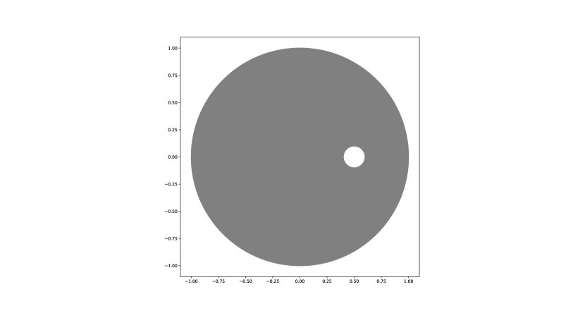
4.1 Test 1: Flow between 2d offset circles

For the first test, we consider a two-dimensional rotational flow obstructed by a circular obstacle with no-slip boundary conditions. Let $\Omega_{1}\subset\mathbb{R}^{2}$, where

$$\Omega_{1}=\{(x,y)\in\mathbb{R}^{2}:x^{2}+y^{2}<1\}\setminus\{(x,y)\in\mathbb{R}^{2}:(x-.5)^{2}+y^{2}\leq.01\}.$$

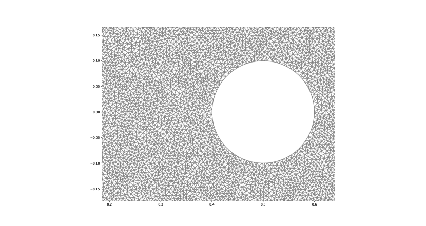
The domain $\Omega_{1}$ is discretized via a Delaunay triangulation with a maximal mesh width of $.01$; a plot is given below. From the plot in Figure 1 of the model’s Taylor microscale this mesh fully resolves the model solution.

(a) $\Omega$

(b) $\Omega$ near the obstacle

Fig. 1: Discretization of $\Omega$

We start the test at rest, i.e., $v_{0}=(0,0)^{T}$, and let the fluid have kinematic viscosity $\nu=0.0001$. We take the final time $T=10$ and averaging window $\tau=1$. Rather than give an interpretation of the time average for $0\leq t<1$ we harvest flow statistics for $t\geq 1$ after a cold start and ramping up the body force with a multiplier $\min\{t,1\}$. To generate counter-clockwise motion we impose the body force

$$f(x,y;t)=\min\{t,1\}(-4y(1-x^{2}-y^{2}),4x(1-x^{2}-y^{2}))^{T}.$$

Initial Conditions. An initial condition for the velocity, $v(x,0)$, and for the TKE $k(x,0)$ must be specified. For some flows standard choices are known. We use a different and systematic approach to the initial condition $k(x,0)$ as follows. From $l(x,t)=\sqrt{2}k^{1/2}\tau$ we set at $t=0,$ $l=l_{0}(x)$ and solve for $k(x,0)$. This yields the initial condition

$$k(x,0)=\frac{1}{2\tau^{2}}l_{0}^{2}(x)\text{ where }l_{0}(x)=\min\{0.41y,0.082\mathcal{R}e^{-1/2}\}.$$

This choice means that $l_{0}(x)=l_{K}(x,0)$.

To compare the models, we plot the temporal evolution of the above statistics. For both models, we let $\mu=0.55$ and timestep $\Delta{t}=.01$. To let the flow develop, we first activate both models when $t=1$.

(a) Model intensity $I_{\text{model}}$

(b) Effective viscosity $\nu_{\text{effective}}$

(c) Viscosity ratio $VR_{1}$

(d) Taylor microscale $\lambda_{\text{Taylor}}$

(e) $avg{(l)}/L$

(f) $avg{(\nu_{T})}/UL$

Fig. 2: 2d Flow statistics for both models.

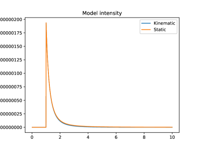
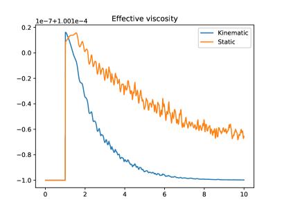
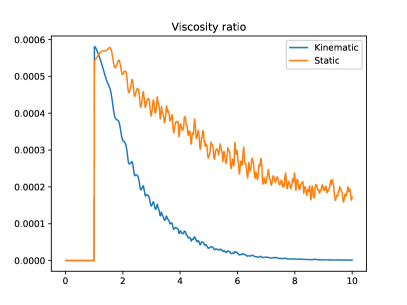
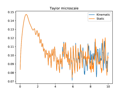
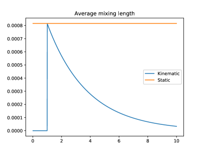
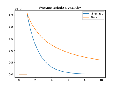
In the test, the model’s estimate of the turbulent intensity for both is similar, as shown in Figure 2a. In [14] the turbulent intensity was estimated by an ensemble simulation. For ensemble averaging $I$ was significant larger than calculated here by time averaging and with the $1-$equation model. Either intensities by time and ensemble averaging do not coincide or $I_{model}$ is not an accurate turbulent intensity. Figure 2b shows that the effective viscosity for the kinematic length scale is significantly smaller than for the standard model. This is consistent with Figure 2c, 2e and 2f. In Figure 2d the Taylor microscale is larger than expected, possibly due to numerical dissipation in the fully implicit time discretization used.

The statistics considered reveal differences in the two models. Figure 2b shows that the kinematic model has an effective viscosity that decays to $\nu_{\text{effective}}=0.0001$ more rapidly than does the static model. More evidence of this fact is given in Figure 2c, which shows the turbulent-to-molecular viscosity ratio. The comparison of the evolution of the Taylor microscale, given in Figure 2d, shows similar profiles until $t\approx 5$. Figure 2e, which compares the evolution of the average mixing length, shows that the kinematic mixing length model decreases the turbulence length scale over the course of the simulation. Finally, Figure 2f shows that the average turbulent viscosity for the kinematic model is consistently smaller than that of the static model. Statistical comparisons of both of these models with different parameters (in particular, the turbulent time scale $\tau$) are also of interest. Below, we give semilog (in the vertical axis) plots of the average mixing length with different values of $\tau$.

(a) $avg{(l)}/L$ for $\tau=.01,.1,1$.

(b) $avg{(l)}/L$ for $\tau=1,10,100$ and the static model.

Fig. 3: Average mixing length comparison

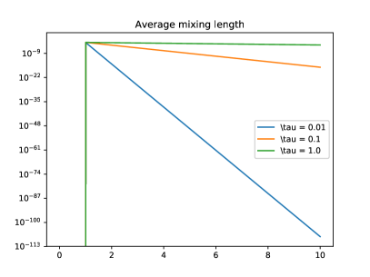
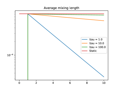
Figure 3 shows that decreasing values of $\tau$ lead to a vanishing average mixing length, whereas increasing $\tau$ yields average mixing lengths that appear to converge to the static mixing length.

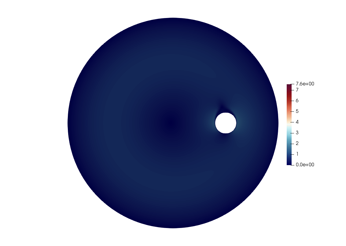
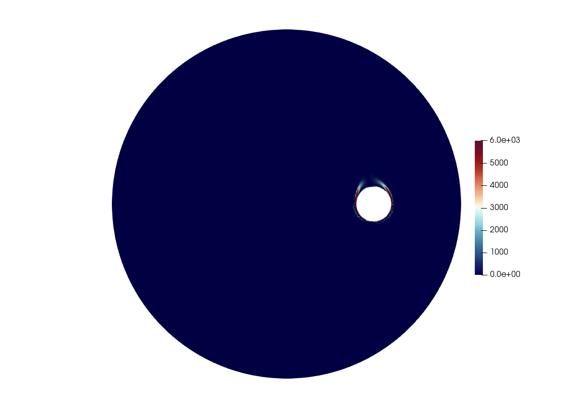
Next, we give plots of the velocity magnitude and squared vorticity for the kinematic model at $t=1,5,$ and $10$.

(a) Velocity $(t=1)$

(b) Squared vorticity $(t=1)$

(c) Velocity $(t=5)$

(d) Squared vorticity $(t=5)$

(e) Velocity $(t=10)$

(f) Squared vorticity $(t=10)$

Fig. 3: Kinematic mixing length model velocity and vorticity.

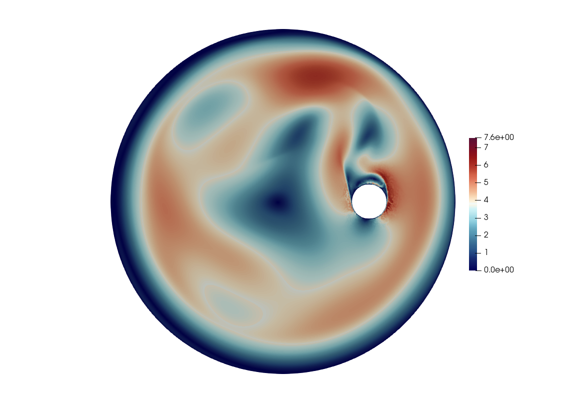
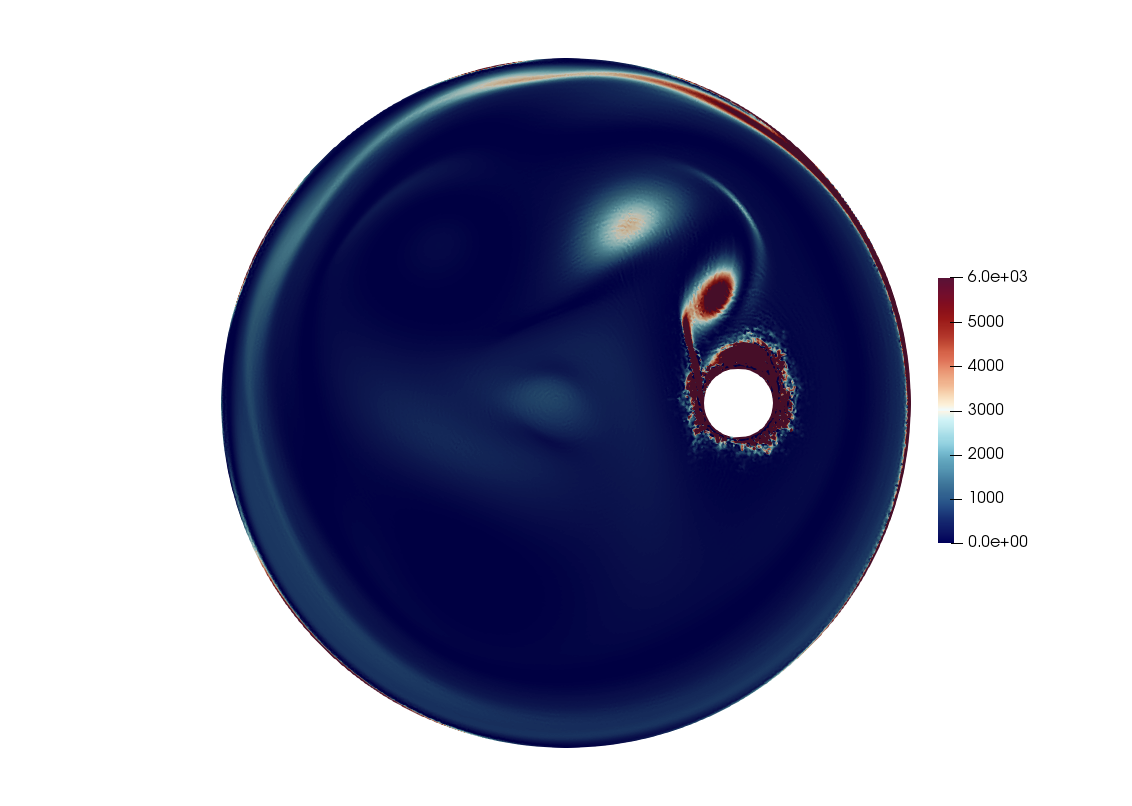
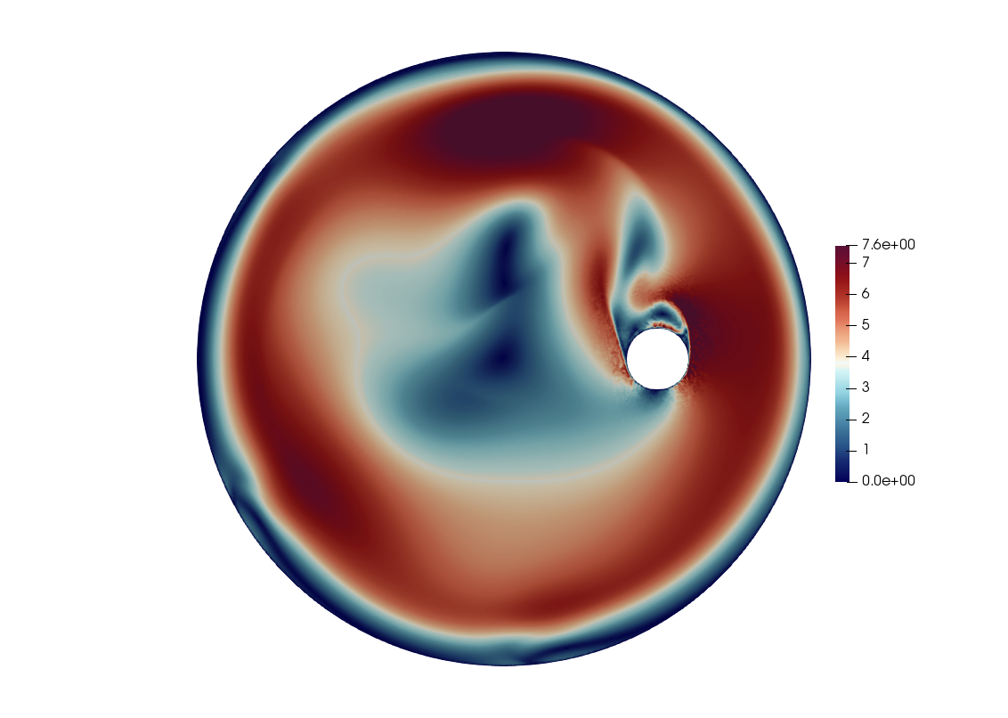
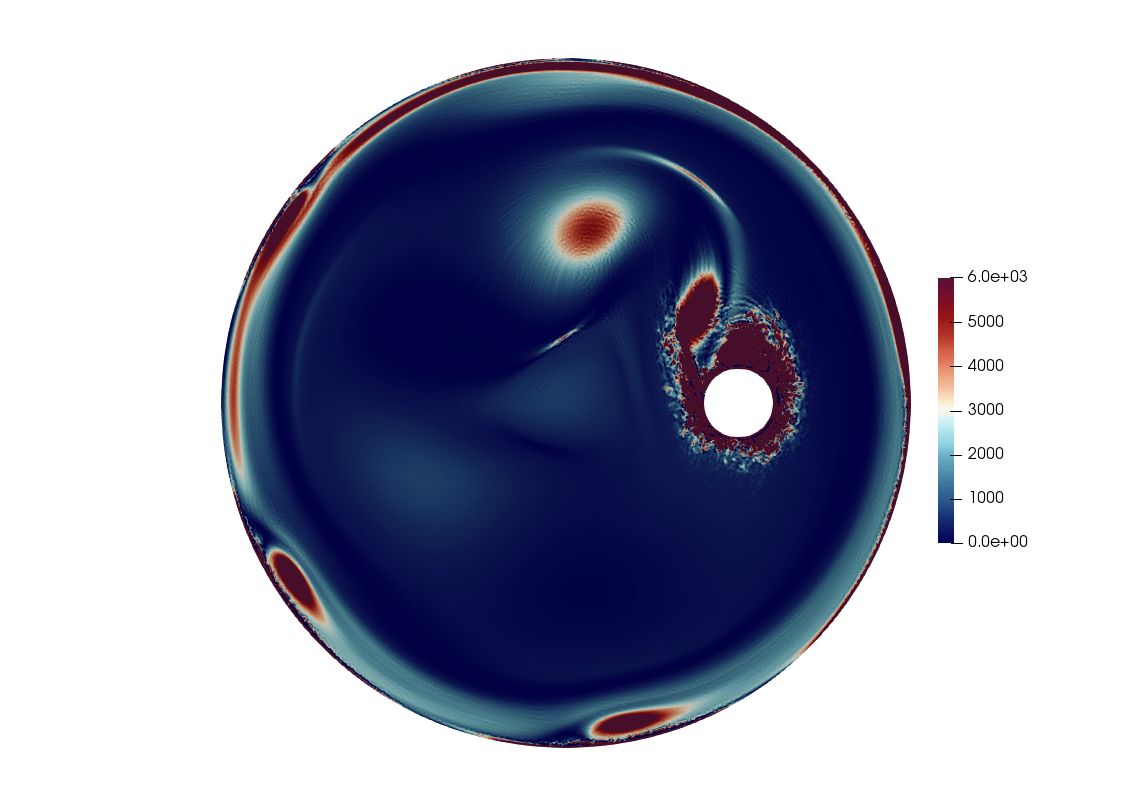
4.2 Test 2: Flow between 3d offset cylinders

The second test is a 3d analogue of the first. It shows similar differences in the two models. Taking $\Omega_{1}$ to be the domain given in the first test, we define $\Omega=\Omega_{1}\times(0,1)$, a cylinder of radius and height one with a cylindrical obstacle removed. The domain $\Omega$ was discretized with Delaunay tetrahedrons with a maximal mesh width of approximately $0.1$. As before, we start the flow from rest $(v_{0}=(0,0,0)^{T})$ and let the kinematic viscosity $\nu=0.0001$. The flow evolves via the body force

$$f(x,y,z;t)=\min\{t,1\}(-4y(1-x^{2}-y^{2}),4x(1-x^{2}-y^{2}),0)^{T},$$

and is observed over the time interval $(0,10]$, with $\Delta{t}=.05$ and the initial conditions for $k$ being set in the same way as the first test. Below, we present the evolution of the statistics introduced above.

(a) Model intensity $I_{\text{model}}$

(b) Effective viscosity $\nu_{\text{effective}}$

(c) Viscosity ratio $VR_{1}$

(d) Taylor microscale $\lambda_{\text{Taylor}}$

(e) $avg{(l)}/L$

(f) $avg{(\nu_{T})}/UL$

Fig. 4: Flow statistics for the 3d offset cylinder problem.

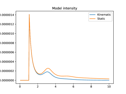
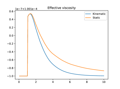
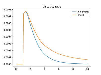
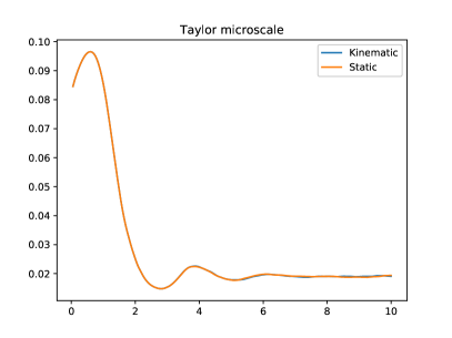
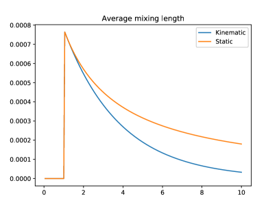
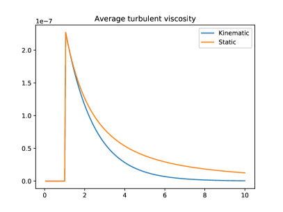
The statistics shown in Figure 4 exhibit similar differences between the 2 models as in the 2d case, Figs. 4a–4c, 4e–4f. As before, the evolution of the Taylor microscale in Figure 4d is similar in both models, with slight differences appearing as the flow evolves. Here the Taylor microscale is much smaller for the 3d test than the previous 2d test (even though the mesh is coarser).

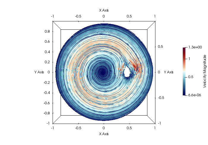
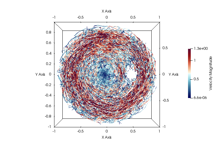
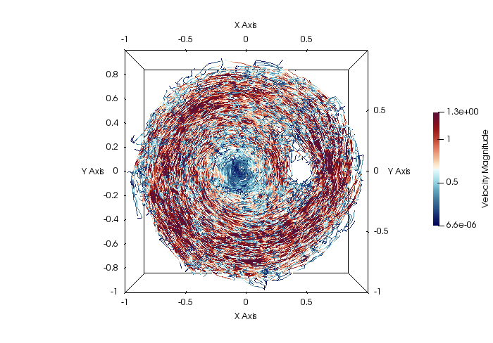
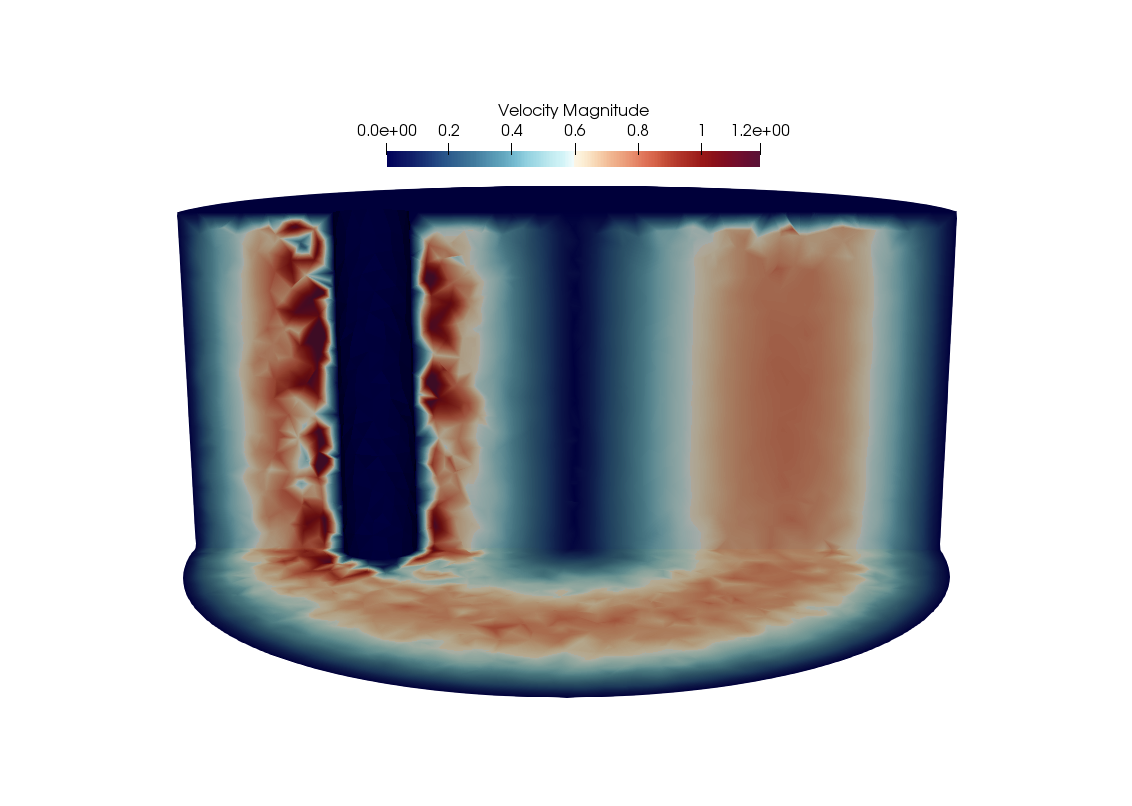
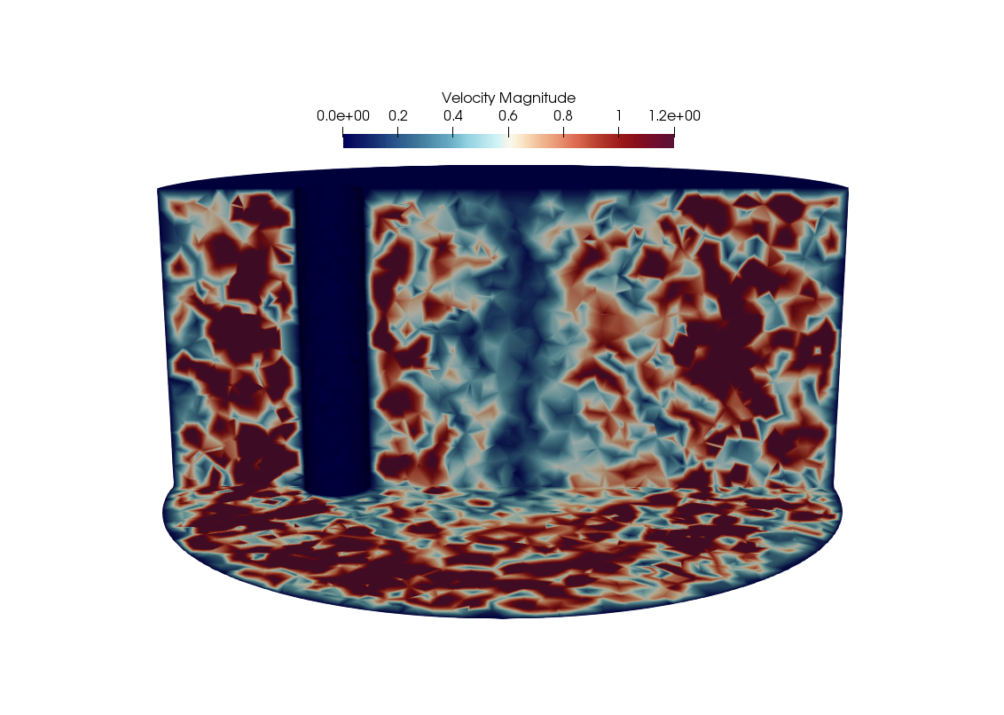
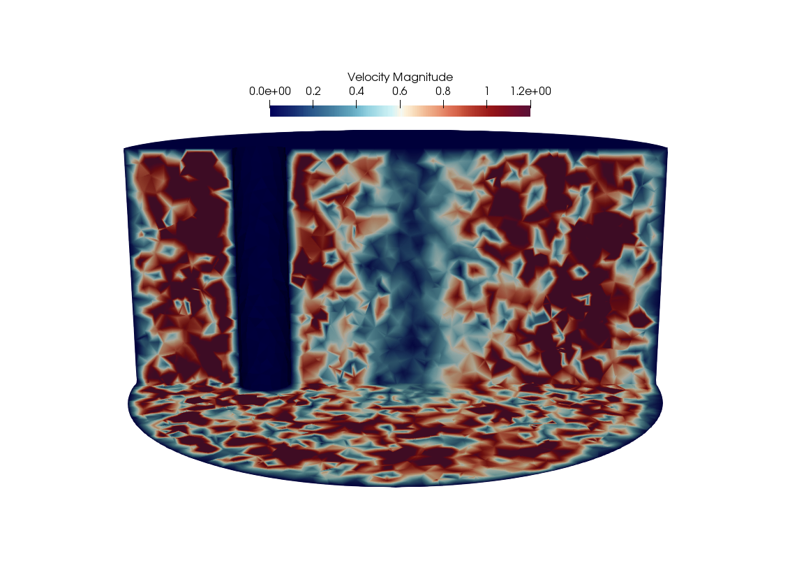
To conclude, we present streamline plots of the offset cylinder simulation as viewed from above. In the figures, color signifies the magnitude of velocity. At $t=1$, the flow appears laminar, and over the course of the simulation becomes turbulent, as evidenced by the plots at $t=5,10$. This behavior can be seen in Figure 6, which views the domain from the positive $y$ direction and considers a slice at $z=.1$.

(a) $t=1$

(b) $t=5$

(c) $t=10$

Fig. 5: Streamlines for the 3d offset cylinder problem.

(a) $t=1$

(b) $t=5$

(c) $t=10$

Fig. 6: Velocity magnitude for the 3d offset cylinder problem.

5 Conclusions and open problems

Predictive simulation of turbulent flows using a URANS model requires some prior knowledge of the flow to calibrate the model and side conditions. Our intuition is that the better the model represents flow physics the less complex this calibration will be. To this end we have suggested a simple modification of the standard $1-$equation model that analysis shows better represents flow physics.

In turbulence, it is of course easier to list open problems than known facts. However, there are a few within current technique for the modified model herein.

• Extension of estimates of $\left\langle\varepsilon_{\text{model}}\right\rangle$ to turbulent shear flows is open and would give insight into near wall behavior. Various methods for reducing the turbulent viscosity locally in regions of persistent, coherent structures have been proposed, e.g., [33], [18] . Sharpening the (global) analysis of $\left\langle\varepsilon_{\text{model}}\right\rangle$ for these (local) schemes would be a significant breakthrough.

• Extension of an existence theory to the modified model is another important open problem. Our intuition is that existence will hold but there may always occur hidden difficulties.

• The estimate in Theorem 1 requires an upper limit on the time average’s window of $\tau/T^{\ast}\leq\mu^{-1/2}$. We do not know if a restriction of this type can be removed through sharper analysis or if there exists a fundamental barrier on the time average’s window. Connected with this question, the behavior of the model as $\tau\rightarrow\infty$ is an open problem.

• Eddy viscosity models do not permit transfer of energy from fluctuations back to means. Recently in [15] an idea for correcting these features of eddy viscosity models was developed. Extension to the present context would be a significant step forward in model accuracy.

• Various averages of the classic turbulence length scale with the kinematic one proposed herein are possible, such as the geometric average

  $$l_{\theta}(x,t)=l_{0}^{\theta}(x)l_{K}^{1-\theta}(x,t).$$

  It is possible that such a weighted combination will perform better than either alone. For example, for decaying turbulence when $v=0,\nabla v=0$ the $k-$equation reduces to

  $$k_{t}+\frac{1}{l_{\theta}}k\sqrt{k}=0.$$

  Decaying turbulence experiments in 1966 of Compte-Bellot-Corsin, e.g., p.56-57 in [22], suggest polynomial decay as $k(t)=$ $k(0)\left(1+\lambda t\right)^{-1.3}$. Neither mixing length formula replicates this decay. But choosing $\theta=\frac{2}{1.3}\simeq 1.54$ yields polynomial decay with exponent $-1.3$. The effect of this data-fitting on the predictive power of the model and on the Conditions 1-4 are an open problem.

• Our intuition is that for many tests numerical dissipation is greater than model dissipation (and acts on different features and scales of those features). Thus the analysis of numerical dissipation including time discretizations is an important open problems.

• Comparative test on problems known to be challenging for RANS and
  URANS models is an important assessment step.

References

- [1] F. Brossier and R. Lewandowski, Impact of the variations of the mixing length in a first order turbulent closure system, ESAIM: Mathematical Modelling and Numerical Analysis 36.2 (2002): 345-372
- [2] M. Bulicek and J. Malek, Large data analysis for Kolmogorov’s 2 equation model of turbulence, Nonlinear Analysis 50(2018) 104-143.
- [3] M. Bulíček, R., Lewandowski and J. Malek, On evolutionary Navier-Stokes-Fourier type systems in three spatial dimensions, Commentationes Mathematicae Universitatis Carolinae 52.1 (2011) 89-114.
- [4] J. Boussinesq, Essai sur la théorie des eaux courantes, Mémoires présentés par divers savants à l’Académie des Sciences 23 (1877): 1-680
- [5] T. Chacon-Rebollo and R. Lewandowski, Mathematical and numerical foundations of turbulence models and applications, Springer, New-York, 2014.
- [6] P. Davidson, Turbulence: an introduction for scientists and engineers. Oxford Univ. Press, 2015.
- [7] O. Darrigol, Worlds of flow, Oxford, 2005.
- [8] C. Doering and C. Foias, Energy dissipation in body-forced turbulence, J. Fluid Mech., 467 (2002), 289-306.
- [9] C.R. Doering and P. Constantin, Energy dissipation in shear driven turbulence, Physical review letters 69.11 (1992): 1648.
- [10] C. Doering and J.D. Gibbon, Applied Analysis of the Navier-Stokes Equations, Cambridge Univ. Press, Cambridge, 1995.
- [11] P.A. Durbin and B.A. Pettersson Reif, Statistical theory and modeling for turbulent flows, Second Edition, Wiley, Chichester, 2011
- [12] M. Eckert, The dawn of fluid dynamics, Wiley-VCH, Weinheim, 2006.
- [13] U. Frisch, Turbulence, Cambridge Univ. Press, Cambridge, 1995.
- [14] Nan Jiang and W. Layton, Numerical Analysis of two Ensemble Eddy Viscosity Models of Fluid Motion, accepted: NMPDEs, 2014, published online : 15 JUL 2014, DOI: 10.1002/num.21908.
- [15] Nan Jiang and W. Layton, Algorithms and models for turbulence not at statistical equilibrium, Computers & Mathematics with Applications, 71 (2016) 2352-2372.
- [16] F.T. Johnson, E.N. Tinoco and N.J. Yu, Thirty years of development and application of CFD at Boeing Commercial Airplanes, Seattle, Computers & Fluids, 34(10):1115–1151,2005.
- [17] W. Layton, The 1877 Boussinesq conjecture: Turbulent fluctuations are dissipative on the mean flow, TR 14-07, www.mathematics.pitt.edu/research/technical-reports, 2014.
- [18] W. Layton, L.G. Rebholz, C. Trenchea, Modular nonlinear filter stabilization of methods for higher Reynolds numbers flow, Journal of Mathematical Fluid Mechanics 14 (2012), 325-354.
- [19] R. Lewandowski, The mathematical analysis of the coupling of a turbulent kinetic energy equation to the Navier-Stokes equation with an eddy viscosity, Nonlinear Analysis, 28 (1997), 393-417.
- [20] R. Lewandowski and B. Mohammadi, Existence and positivity results for the model and a modified model, Math. Model Methods Appl. Sci.3(1993) 195-215.
- [21] J. Mathieu and J. Scott, An introduction to turbulent flows, Cambridge, 2000.
- [22] B. Mohammadi and O. Pironneau, Analysis of the K-Epsilon Turbulence Model, Masson, Paris, 1994.
- [23] A. Pakzad, Damping Functions correct over-dissipation of the Smagorinsky Model, Mathematical Methods in the Applied Sciences 40 (2017), no. 16, DOI 10.1002/mma.4444.
- [24] S. Pope, Turbulent Flows, Cambridge Univ. Press, Cambridge, 2000.
- [25] L. Prandtl, Über ein nenes Formelsystem für die ausgebildete Turbulenz, Nacr. Akad. Wiss. Göttingen, Math-Phys. Kl., (1945) 6-16.
- [26] L. Prandtl, On fully developed turbulence, in: Proceedings of the 2nd International Congress of Applied Mechanics, Zurich (1926) 62-74.
- [27] A.J.C. Saint-Venant (Barré), Note à joindre au Mémoire sur la dynamique des fluides, CRAS 17(1843), 1240-1243.
- [28] P.R. Spalart, Philosophies and fallacies in turbulence modeling, Progress in Aerospace Sciences, 74:1–15, 2015.
- [29] V.P. Starr, Physics of Negative Viscosity Phenomena, McGraw Hill, NY, 1968.
- [30] G.I. Taylor, Eddy motion in the atmosphere, Phil. Trans. of Royal Soc. Series A 215 (1915) 1-26.
- [31] J.C. Vassilicos, Dissipation in turbulent flows, Ann. Rev. Fluid Mech. 47 (2015) 95-114.
- [32] M. Vergassola, S. Gama and U. Frisch, Proving the existence of negative, isotropic eddy viscosity, pp. 321-328 in: Solar and Planetary Dynamics (eds.: M. Proctor, D. Mattheus and A. Rucklidge) Cambridge U. Press, Cambridge, 1994.
- [33] A.W. Vreman, An eddy-viscosity subgrid-scale model for turbulent shear flow: algebraic theory and applications, Phys. Fluids 16 (2004), 3670-3681.
- [34] X. Wang, The time averaged energy dissipation rates for shear flows, Physica D, 99 (1997) 555-563. 2004.
- [35] D.C. Wilcox, Turbulence Modeling for CFD, DCW Industries, La Canada, 2006.
- [36] Zi-Niu Wu and Song Fu, Positivity of k-epsilon turbulence models for incompressible flow, Mathematical Models and Methods in Applied Sciences 12 (2002): 393-406.
- [37] H. Xiao and P. Cinnella, Quantification of Model Uncertainty in RANS: A Review, arxiv.org/pdf/1806.10434.pdf , 2018.