Hidden Markov Models derived from Behavior Trees

Abstract

Behavior trees are rapidly attracting interest in robotics and human task-related motion tracking. However no algorithms currently exist to track or identify parameters of BTs under noisy observations. We report a new relationship between BTs, augmented with statistical information, and Hidden Markov Models. Exploiting this relationship will allow application of many algorithms for HMMs (and dynamic Bayesian networks) to data acquired from BT-based systems.

Submitted to IEEE Transactions on Robotics and Automation, 23-Jul-2019.

1 Introduction

The domain of this paper is tools for representing, observing, and tracking task performance in which the observations or measurements of the task progression are noisy. Applications include monitoring progression of defined tasks performed by a human through noisy measurements. Hidden Markov Models (HMMs) are widely used and well known in applications such as speech[1, 2], surgery[3], and bioinformatics[4]. Behavior Trees (BTs) are a plan representation, arising in the world of Game AI for non-player characters, which are making inroads in robotics [5, 6] and medicine[7].

The contribution of this paper is a new relationship between BTs and HMMs. We show that when a BT is augmented with statistical or prior probability information, then it corresponds to a unique HMM having a specific structure. We can then exploit this link and the well known HMM algorithms for state estimation and system identification to monitor the evolution of a system described by a BT in spite of noisy observations. Useful links then also follow between BTs and Dynamic Bayesian Nets which could improve the power of these methods[8].

1.1 Models

In this work, a HMM having $N$ states and $J$ discrete output symbols is described by

$$HMM=\left\{\begin{array}[]{ll}\Pi_{i}&\in\mathcal{R}^{N}\\ A_{i,j}&\in\mathcal{R}^{N\times N}\\ B_{i,j}&\in\mathcal{R}^{N\times J}\end{array}\right.$$

Where $\Pi_{i}$ is the probability of the initial state being state $i$, $A_{i,j}$ is the probability of transition from state $i$, to state $j$, and $B_{i,j}$ is the probability of symbol $j$ being observed in state $i$. The observations (also called emissions) depend probabilistically on the current state (which is thus not directly observable).

Early work on Hidden Markov Models made a major early advance in speech recognition[1, 2]. Three well-known algorithms, reviewed in[9] and widely used with HMMs, provide useful information from signals arising from a task performance. The Baum-Welch expectation-maximization algorithm tunes the parameters of a HMM to increase the probability that a given data set arises from that HMM. The Viterbi algorithm optimally estimates the most likely state sequence from a given data set based on a HMM, and the Forward Algorithm computes the probability that a given data set was produced by a given HMM. In robotics, Hidden Markov Models have been applied to modeling sequential data arising from manipulation processes[10, 11, 12, 13, 3, 5].

Vector Quantization (VQ)

When the random observations are high dimensional (such as six-axis or more motion/force/torque readings measured experimentally in surgery[14]), they may be compressed into discrete symbols using a vector-quantizer such as K-means clustering[9, 15]. [15] found that a code-book size of 63 code-words performed well with 9-dimensional sensor data recorded from a bowel suturing surgical task.

2 BTs and augmented BTs

BT background

Prior to about 2010, the term “Behavior Tree” was used idiosyncratically by several authors, but around that time a body of literature began to emerge around a tree model of behaviors used by the video game industry for AI-based non-player characters[16, 17]. These BTs assume that units of intelligent behavior (such as decisions or units of action) can be described such that they perform a piece of an overall task/behavior, and that they can determine and return a 1-bit result indicating success or failure. These units are the leaves of BTs. The level of abstraction of BT leaves is not specified by the BT formalism and may vary from one application to another or within a single BT. But BTs are deterministic and do not have well established tools for tracking with noisy data, or parameter identification.

In medical robotics, researchers are turning attention to augmentation of the purely teleoperated existing systems such as the daVinci^TM surgical robotic system (Intuitive Surgical, Sunnyvale, CA) with intelligent functions[18, 19]. In this context, BT leaves can represent autonomous robotic functions such as a guarded move, a precision cutting action, acquisition of an ultrasound image, creation of a plan, etc. Earlier medical robotics systems containing automation, such as Robodoc[20] represented task sequences with scripting languages.

Recent literature has applied BTs to UAV control[21], humanoid robotic control[22], and human-robot cooperation in manufacturing[5]. Theoretical classifications of BTs have been conducted by several authors which formally relate BTs to Finite State Machines (FSMs)[6] yielding advantages of modularity and scalability with respect to FSMs. Other theoretical studies have related BTs to Hybrid Dynamical Systems[23], and have developed means to guarantee correctness and composability of BTs[24]. Software packages and Robotic Operating System (ROS, [25]) implementations are now available[26]. Several of the above authors have developed graphical user interfaces with which humans (such as domain experts) can create, visualize, and edit BTs. The reader is referred to the above references for ample introductory material and examples of BT concepts.

Figure 1: A simple Behavior Tree example. Leaves $l_{1}$ and $l_{2}$ belong to a Sequence ($\to$) node and $l_{3},l_{4}$ to a selector (?). If $l_{1}$ fails, control passes to $Out_{F}$. If $l_{1}$ and then $l_{2}$ succeed, control passes to the Selector (?) node which starts $l3$ etc.

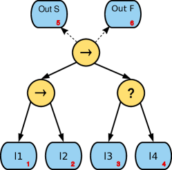
When representing a process with BTs, the analyst breaks the task down into modules which are the leaf nodes of the BT. Every BT node must return either Success or Failure when called by its parent node. All higher level nodes in the BT define composition rules to combine the leaves including: Sequence , Selector , and Parallel node types. A Sequence node defines the order of execution of leaves and returns Success if all leaves succeed in order, returning Failure at the first child failure. A Selector node (also called “Priority” node by some authors) tries leaf behaviors in a fixed order, returns success when a node succeeds, and returns failure if all leaves fail. A Parallel node starts all its child nodes concurrently and returns success if a specified fraction of its children return success. Further refining the behavior tree, “Decorator ” nodes have a single child and can modify behavior of subsequent branches with rules such as “repeat until Success”.

Applied to robotics, BTs have been explored in the context of humanoid robot control [26, 27, 28], human-robot collaborative control[5], and as a modeling language for intelligent robotic surgical procedures [18, 19].

2.1 ABT definitions

Augmented BTs

With experience comparing real task execution traces with a BT representing the task, we can learn that some leaves may succeed infrequently or all the time. Let $iS$ be the event where leaf $i$ succeeds and $iF$ the event where it fails. To incorporate information about $iS$ statistics, we define an Augmented Behavior Tree, or ABT.

$$ABT==\{BT,P_{l},B_{(l+2)\times m}\}$$ (1)

where $P_{l}=[ps_{1},ps_{2},\dots,ps_{l}]^{T}$, $ps_{i}=P(iS|state=i)$ and $l$ is the number of BT leaves or states. We add two “output states”, $O_{S},O_{F}$ to the states defined by the BT leaves to indicate the final output of the BT root node giving $l+2$ total states. $B_{l+1},B_{l+2}$ are the observation probability distributions for each special output state. Note that these states are not nodes of the BT. We initially assume that the observation is independent of Success  and Failure  . We can get initial values for $P_{l},B_{l+1},B_{l+2}$ from experience, or estimate them from expert knowledge.

For example, assuming expert-labeled sensor data is collected from experiments or experience, we can accumulate a frequentist estimate of $p_{i}$ for each leaf by computing $\hat{p}s_{i}=n_{iS}/n_{i}$, where $n_{iS}$ is the number of times node $i$ returned Success  , and $n_{i}$ is the total number of times node $i$ was executed.

3 Mapping Augmented BTs to HMM

Here we derive a few results on which we can ground the link between ABTs and HMMs. We restrict the types of permitted BT nodes to leaves, Selector , and Sequence nodes. Decorator and Parallel nodes will be considered in below (Section 3.7)

3.1 For each ABT, there is a unique HMM

Proof:

1. Assume the ABT has $l$ leaves, numbered from left to right. Left to right is the conventional direction used by selector ($\to$) and sequence (?) nodes in the BT literature.

2. Create a HMM state for each ABT leaf, and two additional terminal HMM states, $O_{S}$ and $O_{F}$, representing overall success or failure of the ABT, so that the HMM dimension is $N=l+2$.

3. By definition of BT nodes, for each leaf, $j$, belonging to a specific BT, there is a unique successor leaf to which the BT will transition on success, $S_{s}$ and a second leaf/HMM state to which it will transition on failure, $S_{f}$.

4. Because of the left to right structure of Step 1, if the system is in state $j$ (i.e. running leaf $j$), then

   $$S_{s}>j\;\mathrm{and}\;S_{f}>j$$

5. Thus the resulting HMM transition matrix, $A$ will be $N\times N$, upper diagonal, and each row will contain exactly 2 non zero entries $S_{s}$ and $S_{f}$ such that $A_{j,Ss}\neq 0,\quad A_{j,Sf}\neq 0,\quad A_{j,Ss}+A_{j,Sf}=1$ and $A_{j,Ss}=P(S)_{j},A_{j,Sf}=1-P(S)_{j}$

6. The HMM observation densities $B_{j}$ are the same as the ABT observation densities.

7. We can thus construct a unique HMM for each ABT.

3.2 There is more than one BT for each HMM derived above.

Proof:

1. Element $A_{i,j}$ is defined above as the probability of a transition from State $i$ to State $j$, however, it does not contain information about whether the transition is associated by the BT with Success or Failure of the leaf $i$.

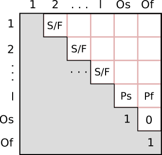
2. We thus will sometimes augment the HMM $A$ matrix to

   $$A_{i,j,k}=P(i\to j|O_{i,k}),k\in\{1,2\}$$

   Adding the outcome, $O_{i,k}\in\{0,1\}$, where $O_{i,1}=1$ if the outcome of leaf $i$ is Success , and $O_{i,1}=0$ if the outcome of leaf $i$ is Failure . Since $O_{i,1},O_{i,2}$ both correspond to the Success / Failure outcome of state $i$, and only one is true, we have $O_{i,2}=1-O_{i,1}$ and either $O_{i,1}$ or $O_{i,2}$ must be 0.

3. Thus for each row in $A$, containing two non-zero probabilities which add to 1, there are two permutations, S/F and F/S, giving more than one BT.

4. When augmented as in Step 2, there is only one BT for each HMM (which follows the constraints in 3.1).

3.3 Proposition

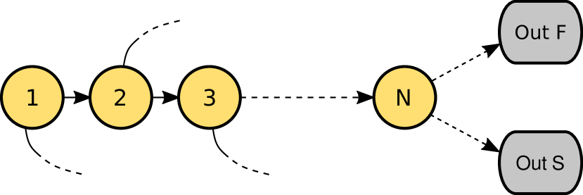
In the state evolution of a BT, there is at least one possible pathway (determined by S/F outcomes of the leaves) in which all $l$ leaves are executed in numerical order (Figure 2(a)) such that the BT visits each leaf in turn.

(a)

(b)

Figure 2: (a) Any BT must have a sequential pathway for a certain set of S/F outcomes. (b) Constraints on $A$ matrix of HMM derived from BT.

Proof:

1. Assume all leaves must have at least one input path. If any leaf has no input path, then it will never be executed and should not be in the BT.

2. By convention, BT leaves are numbered from left to right.

3. Each leaf can belong to a Selector or Sequence parent node.

4. If leaf $j$ is not the last (rightmost) leaf of its parent then the proposition for leaf $j\to j+1$ is trivial by the definition of Sequence and Selector nodes.

5. If leaf $j$ is the last (rightmost) leaf of a Sequence or Selector, and control is passed to that leaf, then the parent’s result is the same as the leaf’s result, also by definition of Sequence and Selector nodes.

6. For any Sequence or Selector node which is a parent of leaf $i$, at least one path from that node must go to a leaf $j>i$ (unless leaf $i$ is the rightmost node in the entire BT).

7. If the leaf is not rightmost of the leaves belonging to its parent, then the result is trivial.

8. If the parent IS rightmost, then by induction it will lead either to one of the two Output states (the root node returns and the BT execution is over) or to another higher level node as non-rightmost.

9. Thus there must be a path from node $i$ to $i+1$.

3.4 Implication

Considering these results, the following constraints define the set of HMM State-Transition-Matrices ($A$) which correspond to an Augmented BT:

1. $A$ must be upper diagonal (3.1 steps 4,5).

2. $A$ must have exactly 2 non-zero entries per row (3.1 steps 4,5).

3. $A_{i,i+1}\neq 0$ (3.3).

3.5 How many BTs are possible for $l$ BT leaves?

1. Since there is a unique HMM for each BT, we can answer the equivalent question: “How many HMMs of $l+2$ states meet the constraints of 3.4?”

2. Each element just above the diagonal, $A_{i,i+1}$, must be non-zero because every BT has a sequential pathway. But further, the probability in $A_{i,i+1}$ may represent Success (if leaf $j$ belongs to a Sequence Node) or Failure (if leaf $j$ belongs to a Selector Node). However, the last leaf, leaf $l$, must transition to Os on Success (and to Of on Failure), so there are $2^{l-1}$ permutations of S/F outcomes for leaves $i=1..l$ (Fig. 2(b)).

3. There must be 2 non-zero entries per row. At this step we ignore their Success/Failure status which was taken into account in steps 1 and 2.

4. For row 1, there are $l+2$ columns, but the $A_{1,1}$ element must be zero, and we have already taken into account the $A_{1,2}$ element. Thus there are $l+2-2=l$ available columns, only 1 of which can be non-zero.

5. For row $i$, there are $l+2-(i+1)=l+1-i$ columns from which to independently choose.

6. Thus there are

   $$\Pi(l,l-1,\dots 2,1)=l!$$

   permutations of the second non-zero elements in rows $1\dots l$.

7. Combining, the total number, $m_{BT}$, of BTs for an $l\times l$ $A$ matrix (augmented with the $O_{S},O_{F}$ rows and columns) would be

   $$m_{BT}=2^{l-1}l!$$

For 10 leaf nodes there are about 1.86 billion possible behavior trees.

3.6 Decodability

As noted above, HMM state decoding can be trivial if the emission probability densities do not overlap, and impossible if they are identical. To achieve a compromise, we defined the emission probability over a set of observation symbols for state $i$ as a normal distribution with parameters $\mu_{i}=i\times R\sigma,\sigma=2.0$ and $\Delta\mu=|\mu_{i}-\mu_{i+1}|$ where $\Delta\mu$ is a constant and the ratio $R$,

$$R=\frac{\Delta\mu}{\sigma}$$ (2)

is a chosen parameter similar to the Z-score of statistics, which parameterizes the degree to which the states are “hidden” by the random observations. We can term this property the “decodability” of the HMM. $R=0$ (no decodability) corresponds to completely hidden states and $R=\infty$ corresponds to a trivial state decoding situation (perfect decodability).

A more general notion of the decodability of HMM output densities is needed in order to apply the proposed methods to experimental data which is likely to be non-gaussian. For example, if codewords are generated by vector quantization of multidimensional sensor signals, they are unlikely to be distributed as described above and in particular, unlikely to be confined to a limited region (e.g. $\approx\mu_{j}\pm 4\sigma$ for state $j$) of symbol indeces. Thus we will apply Kulback Leibler (KL) and Jensen-Shannon (JS) divergence measures to compare the degree to which distributions $B_{i}$ are similar from state-to-state. Applied to the discrete distributions, we use the KL divergence for two state observation densities, $B_{1,j}$ and $B_{2,j}$ as

$$D(B_{1}||B_{2})=\sum_{j=1}^{NSYMBOLS}B_{1,j}\log_{2}\left(\frac{B_{2,j}}{B_{1,j}}\right)$$

Modifying the KL divergence to achieve symmetric and finite properties, we get the JS divergence:

$$JSD(B_{1}||B_{2})=\frac{1}{2}D(B_{1}||M)+\frac{1}{2}D(B_{1}||M)$$

where $M=\frac{1}{2}(B_{1}+B_{2})$. We can also create a measure of the divergence between the set of all $N$ observation densities as

$$JSD(B_{1},\dots,B_{N})=H\left(\sum_{i=1}^{N}w_{i}P_{i}\right)-\sum_{i=1}^{N}w_{i}H(B_{i})$$

where $w_{i}$ are a set of weights on the densities (uniform, $w_{i}=1/N$, in our case) and $H(P)$ is the Shannon Entropy of distribution $P$.

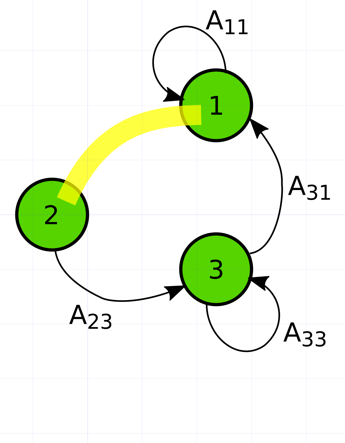
Of note, if the KL or JS divergence between two states is zero, it does not mean the states are completely invisible, depending on the transition probabilities. For example, consider a three state model of Figure 3(a) (Left) in which $JSD_{12}=0$ but $JSD_{13}=JSD_{23}=0$, and furthermore,

$$A=\begin{bmatrix}{}1&0&0\\ 0&0&1\\ 0.5&0&0.5\\ \end{bmatrix}$$

Since there is no transition possible between the states with identical observation densities, it is still possible to distinguish them.

(a)

(b)

Figure 3: (a) Example HMM in which states (separated by yellow arc indicating $D_{12}=0$), and solid arcs show state transitions with finite probability. (b) Workflow for validation of Baum-Welch parameter identification with ABT-derived HMMs using the Baum-Welch algorithm of the hmmlearn.fit() method. The HMM parameters are directly derived from the ABT parameters. HMM parameters are perturbed from 0-50% and also randomized. RMS_error is the RMS difference of the non-zero elements of two HMM transition matrices.

3.7 Behavior Tree Refinements

The basic combinatorial nodes of the BT are Sequence and Selector . In most of this work we limit consideration of BTs to those composed of leaves and these two nodes. However many BT implementations also use “Decorator” nodes for additional functions including

• Repeat until Success nodes

• Parallel nodes

This section will develop the rules to convert BT sections containing Repeat until Success and Parallel nodes into HMMs.

Repeat until Success Decorator

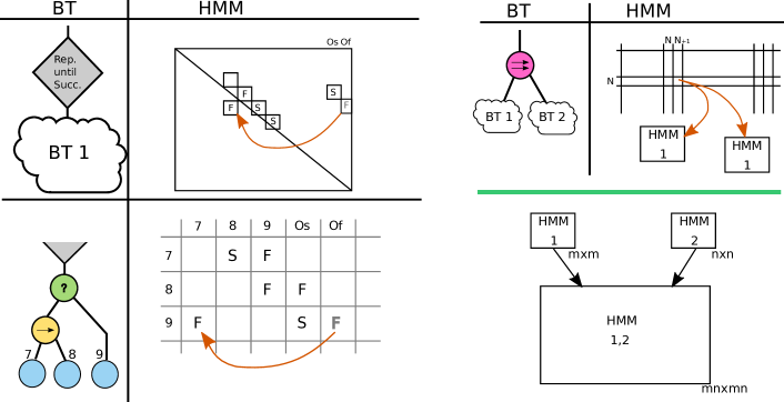
This decorator is applied to a child BT and repeatedly restarts that BT until its one child returns Success . It is straightforward to add the Repeat until Success Decorator to a HMM if we relax the constraint from 3.1, steps 4,5, that the state transition matrix, $A$, be upper diagonal. A BT which is a child of a Repeat until Success Decorator , BT_C, can be inserted into the HMM $A$ matrix as follows:

1. Assume the first leaf of the child BT_C is numbered leaf $k$ in the main BT (to which it is attached through the Repeat until Success Decorator ) and that its subsequent leaves are numbered $k+1,k+2,\dots$.

2. Enter the Success and Failure probabilities for leaves $k+i$ as described in 3.1.

3. Replace any Failure state transition (e.g. non-zero probability associated with failure) in BT_C which would cause BT_C to return Failure , with a transition back to state $k$.

This is illustrated by the example in Figure 4, Left. As an example, a three state BT_C where $k=7$ is shown. The failure of leaf C, resulting in the failure of BT_C is moved to be a transition back to state 7.

Figure 4: Mapping of Repeat until Success Decorator to HMM (Left) results in non-zero terms below main diagonal of HMM state transition matrix, $A$. Mapping of Parallel node to HMM (Right) launches multiple child BTs in parallel, combined into a larger HMM submatrix HMM_1,2.

Parallel Decorator

A Parallel Decorator launches multiple child BTs into concurrent execution. The Parallel node is configured to return Success when a specified fraction of its children return Success . The process to add a Parallel Decorator is illustrated conceptually in Figure 4 (Right). A node corresponding to the Parallel node is shown at row $N$ with two children, BT1 and BT2. The function of the parallel node is to launch multiple HMMs corresponding to BT_C trees, BT1 and BT2. Since the child BTs are executing in parallel, in order to fold them into the main HMM, we must create a set of combined states representing the product of HMM1 and HMM2. To continue this 2-way example, if BT1 has $m$ leaves and BT2 $n$ leaves, the new combined HMM will have $m\times n$ states. Each new state corresponds to a pair of BT1/BT2 leaves. Each row corresponding to the product-HMM will no have 4 non-zero entries corresponding to:

	BT1,$l_{i}$	BT2,$l_{j}$
1	S	S
2	S	F
3	F	S
4	F	F

Where $l_{i}$ refers to the leaves of each sub-BT, $1<i<m$, $1<j<n$. More generally, a parallel node with $K$ children, BT_k, each BT having $l_{k}$ leaves, will generate a square submatrix in the overall BT’s $A$ matrix having

$$\prod_{k=1}^{K}l_{k}$$

states (rows and columns).

This significant expansion of the number of states in the HMM, as well as the increase from 2 to 4 non-zero entries in rows, may limit the practical usefulness of HMMs derived from BTs which make use of parallel nodes.

4 Computational Experiments

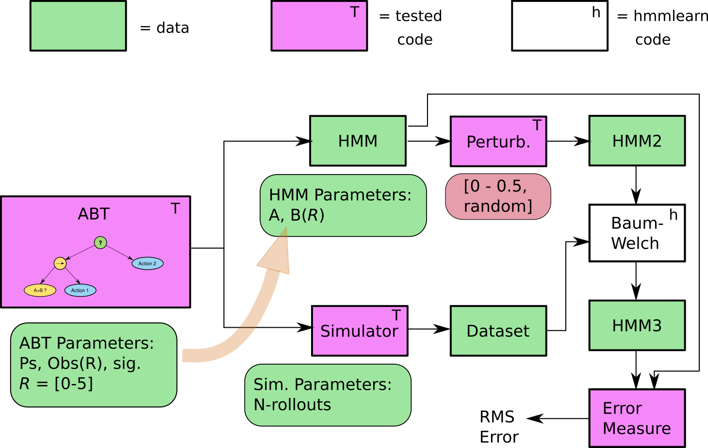
In this section we evaluate the ability of HMM-derived algorithms to work with ABTs. Ultimately, as with HMMs, much depends on the values of HMM/ABT parameters, especially the degree to which the states are “decodable” (Section 3.6). To parameterize the feasibility of these computations, we take two approaches.

First, we perturb the HMM parameters prior to their use with the HMM-based algorithms. For example, we test the ability of the Viterbi decoder to identify the sequence of ABT/HMM states with a model that is perturbed from the model which generated the ABT rollouts and observations. The perturbation was applied to each row of the HMM transition matrix as follows: for a perturbation $0<\tilde{p}<0.5$, let $p_{1}$ be the first (lowest index) non-zero element of each row, and $p_{2}=1-p_{1}$ is the second non-zero element. Then the two non-zero elements are modified as $p_{1}\leftarrow\max(0.95,(1+\tilde{p}\times r)p_{1})$ and $p_{2}=1-p_{1}$, $r\in\{-1,+1\}$ is a random sign variable drawn with 0.5 probability on each sign. Because it is frequently done in HMM research, for comparison we created another HMM transition matrix by initializing all HMM elements to random values [0.0-1.0) (subject to each row totaling 1.0). Second we study performance under various levels of “decodability” of the HMM states, by generating data sets with values of $R$ from the set $\{0,0.25,1.0,2.5,5.0\}$. Simulations were generated from 6-state and 16-state BTs to explore the effect of model size.

For the two ABTs, we generated simulated traces of 15,000 state (leaf) sequences and their associated random emissions by running ABT Monte-Carlo simulations. Results did not change when more than 15,000 sequences were generated. State evolution of the ABTs was determined by the success/fail probability of each leaf, $ps_{i}$ (Section 2.1), and emissions determined by the observation density associated with each leaf $B_{ij}$. We implemented the simulation study in Python 2.7 using a modified version of the b3 Behavior Tree library[26, 29]. We added a new leaf class to b3, abt_leaf(b3.Action) which inherits the Action class (BT leaf) and adds data to represent the probability of Success and Failure , as well as a probability of discrete observations/emissions from the leaf.

5 Results

5.1 Relationship to idealized emission probability densities

We computed the KLD & JSD divergence measures for the $B_{ij}$ and compared them with several values of $R$, eqn(2) ( Table 1). The maximum theoretical value of $JSD_{ALL}$ is $\log_{2}(N)$ where $N$ is the number of HMM states ($l+2$) in our application. For the two cases in Table 1, these values are $\log_{2}(6)=2.585$, and $\log_{2}(16)=4.0$. Thus when $R=5$ the observation distributions are essentially distinct.

Table 1: Measures of “decodability”. Relationship between ratio $R$ (2), and $KLD$, $JSD$ divergences between two consecutive state distributions, and $JSD_{ALL}$ between all pairs of states. Measures are evaluated for both 6-state and 16-state models.

Ratio	N	$KLD$	$JSD$	$JSD_{ALL}$	N	$KLD$	$JSD$	$JSD_{ALL}$
0.00	6	0.00	0.00	0.00	16	0.00	0.00	0.00
0.25	6	0.18	0.04	0.12	16	1.62	0.32	0.60
1.00	6	2.89	0.49	0.95	16	22.87	0.99	2.11
2.50	6	17.47	0.98	1.98	16	26.85	1.00	3.32
5.00	6	26.85	1.00	2.54	16	26.85	1.00	3.95

5.2 Forward Algorithm

Figure 5: HMM Forward Algorithm: Log Probability with respect to simulated data vs. Output Ratio and perturbation. Upper Traces: 6-State Model, Lower Traces: 16-State Model.

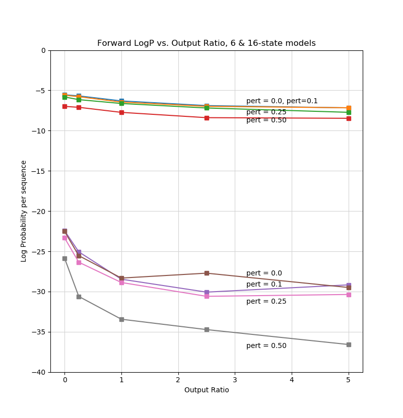
The forward algorithm was applied to 20,000 runouts of observation symbol data generated by several 6-state and 16-state ABT-like HMMs in which the output Observation Ratio, $R$, was varied between 0 to 5.0 to represent the completely hidden state case ($R=0$) and the transparent state ($R=5$) cases.

The models used to generate the runout data were perturbed by [0, 0.1, 0.25, and 0.5] ratios (Section 4). For each combination of output ratio and perturbation ratio, we computed the log probability (logP) of observing each sequence in the simulated data set. Log probability was divided by number of observation runouts to get an average log probability per sequence (Figure 5). For the 6-state ABT-like model, logP per sequence was much higher than for the 16-state model. As expected, logP declined as the perturbation (indicating distance between the data generating and the data evaluation models) increased. logP declined as output ratio, $R$, increased (approx -15% for 6-state model and -30% for 16-state model). This decline may seem counter intuitive, but perhaps is explained by the state transition sequence having less flexibility for the forward algorithm to fit.

5.3 Viterbi State Decoding

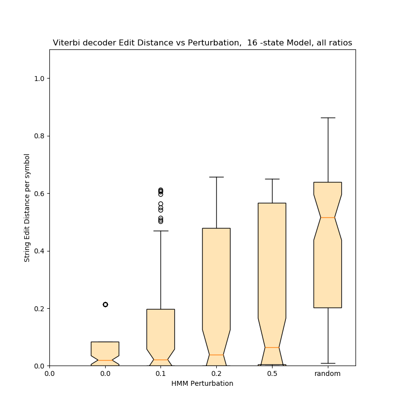
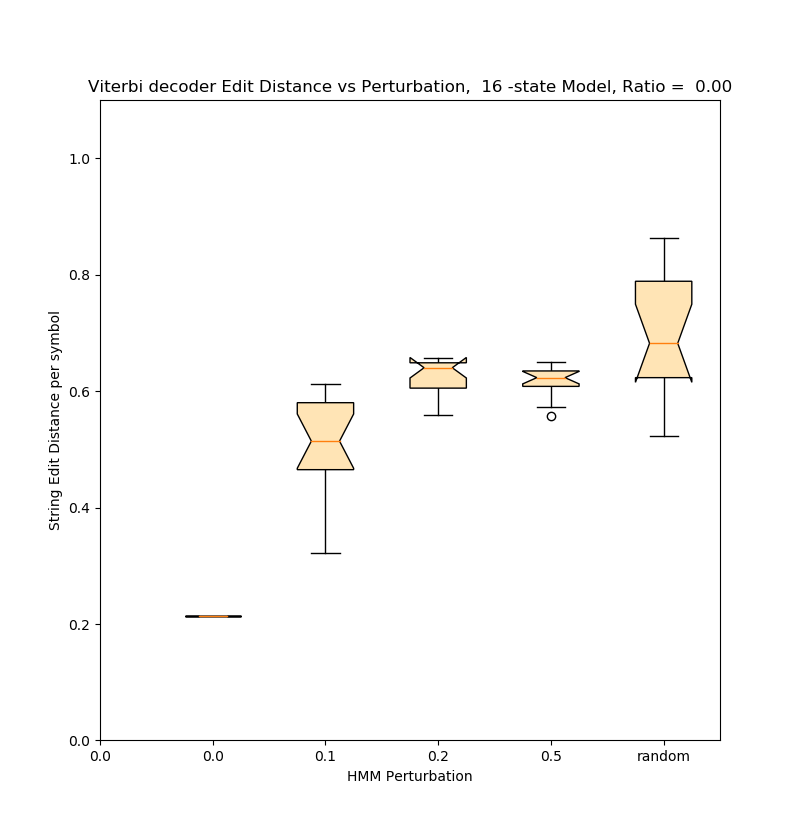
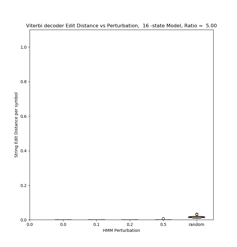
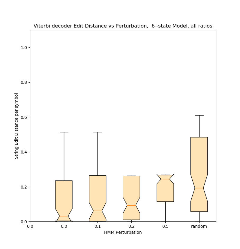
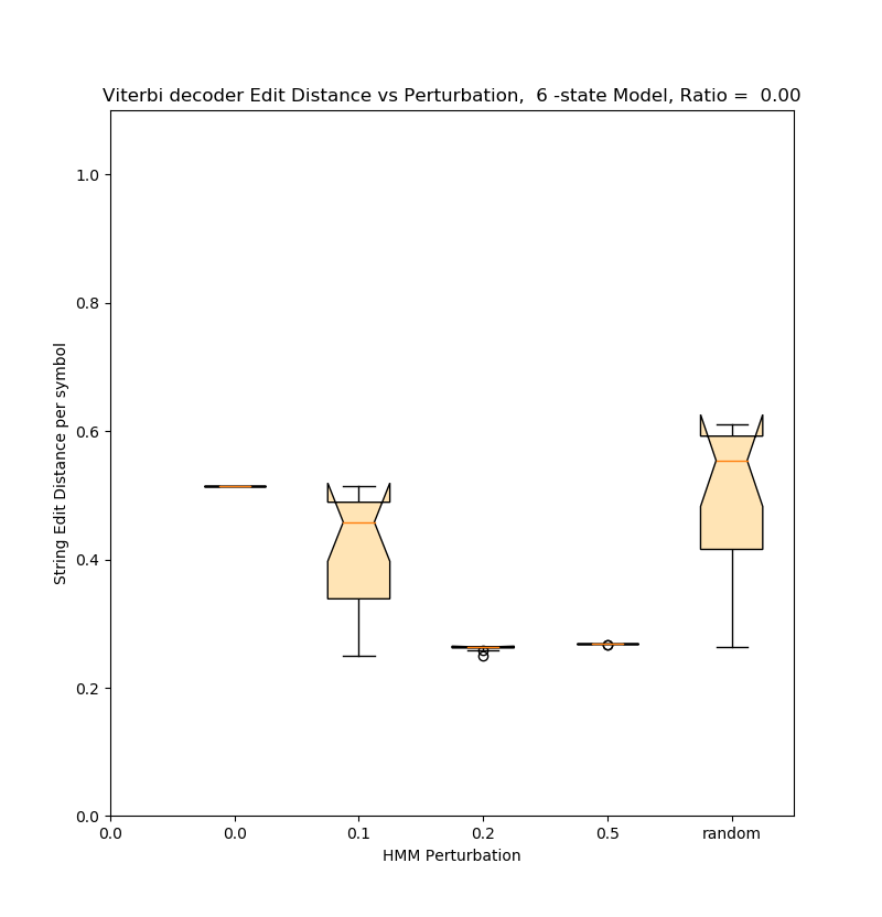
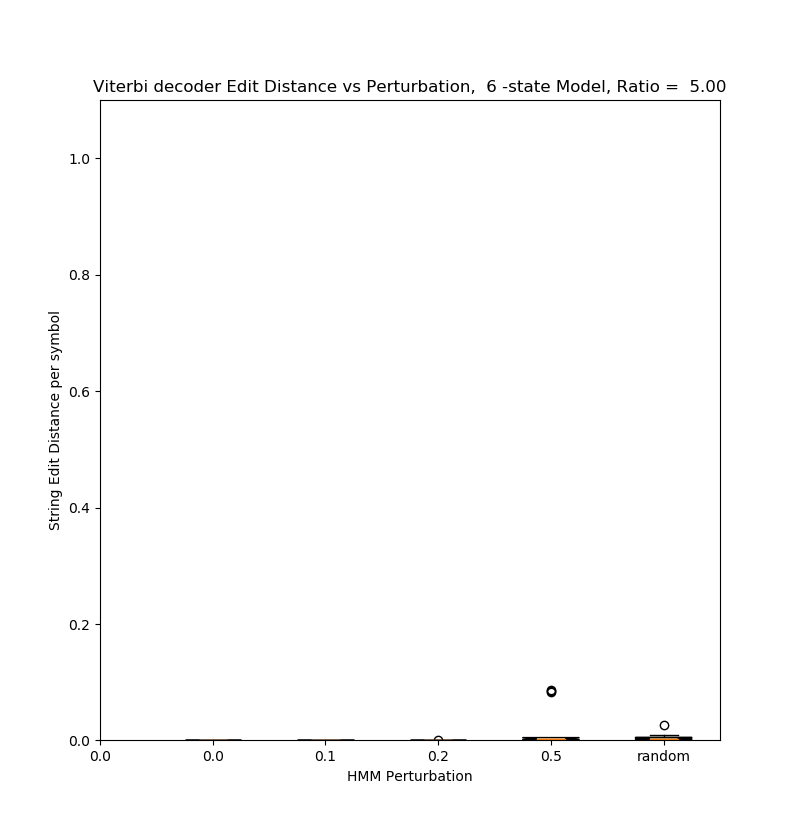
Simulated state evolution data, generated by a reference ABT model, was read by the hmmlearn Viterbi decoder. The state sequence produced was then compared with the true state sequence using the string edit distance (Levenshtein distance [30]) between the estimated and true state sequences divided by the number of symbols. The expected result is that Viterbi decoding by the HMM with zero perturbation of parameters will give the lowest average string edit distance. The simulation data was also input to the Baum-Welch algorithm to assess parameter identification performance when initialized with a perturbed version of the reference model.

(a)

(b)

(c)

(d)

Figure 6: Viterbi Algorithm state tracking error (string edit distance per symbol, SED) of 16 state model. Upper Left: SED vs Ratio, $R$, for all model perturbations. Lower Left: “hard” models ($R=0$, all states have same observation density). Upper Right: SED vs Model perturbation, all ratios. Lower Right: “easy” models ($R=5$, symbols are 5 standard deviations apart).

16-State Model

(a)

(b)

(c)

(d)

Figure 7: Performance of the Baum-Welch Parameter Identification algorithm on a 16 state model against ABT derived sequence data set and associated HMM. Upper Left: BW errors vs Ratio, $R$, for all model perturbations. Lower Left: “hard” models ($R=0$, all states have same observation density). Upper Right: Error vs Model perturbation, all ratios. Lower Right: “easy” models ($R=5$, symbols are 5 standard deviations apart).

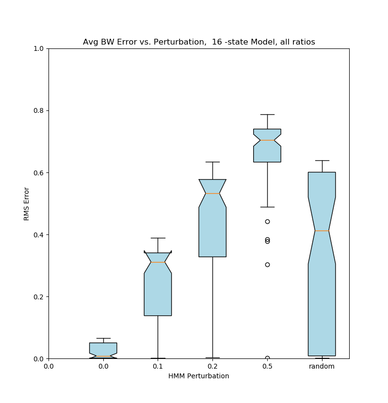
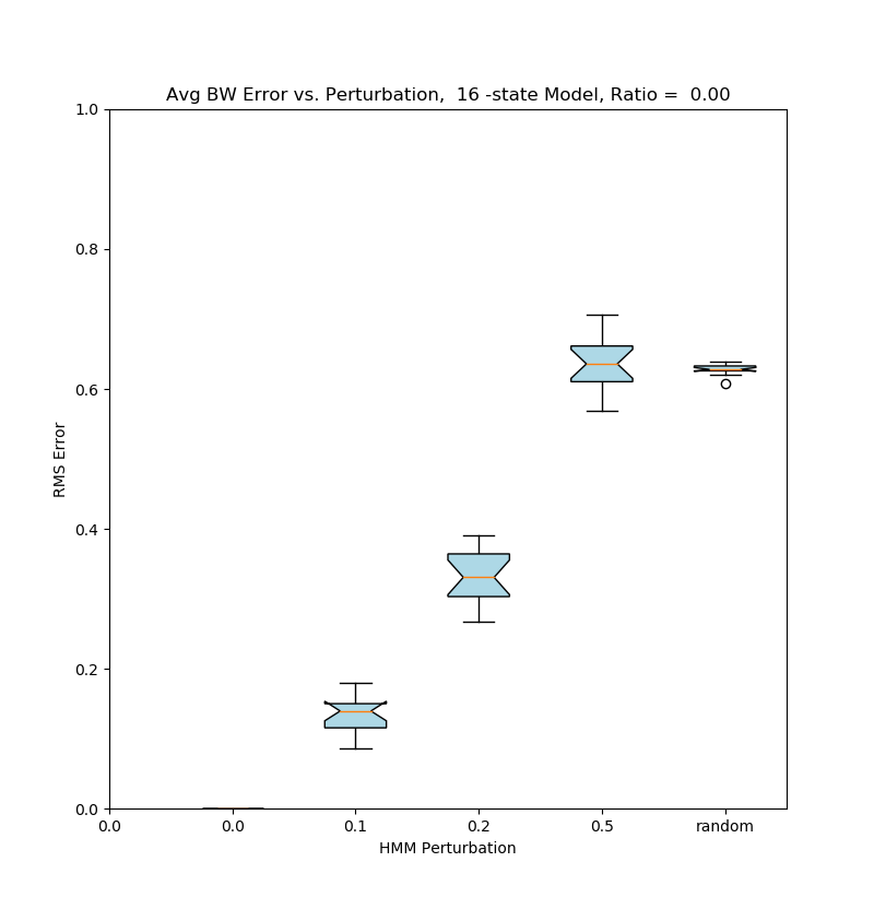
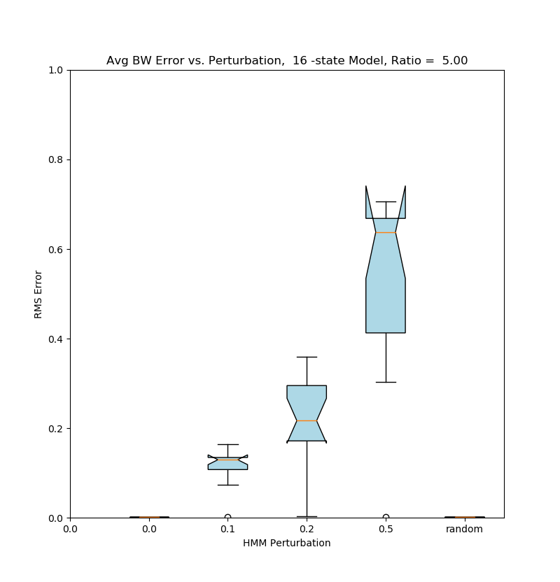
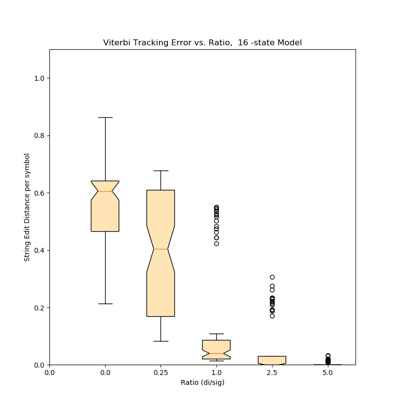
Referring to the yellow box plots of Figure 6, state tracking performance measured by average Levenshtein distance, improves as the observation ratio, $R$, increases (essentially perfect, as expected, for $R=5$), and degrades as the model is perturbed away from the reference model.

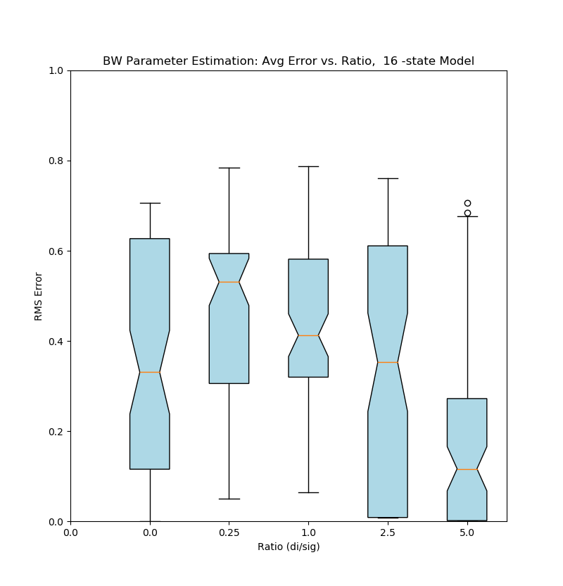
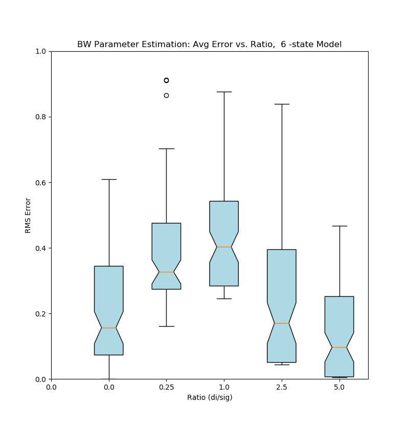
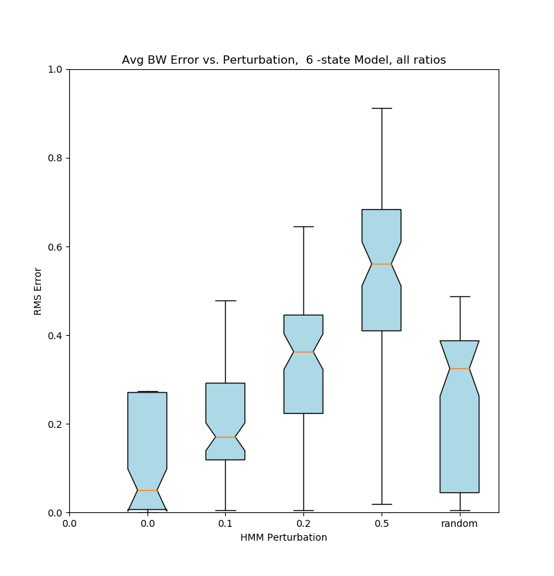
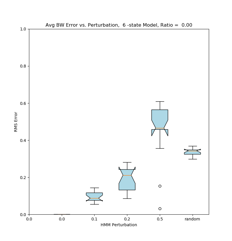
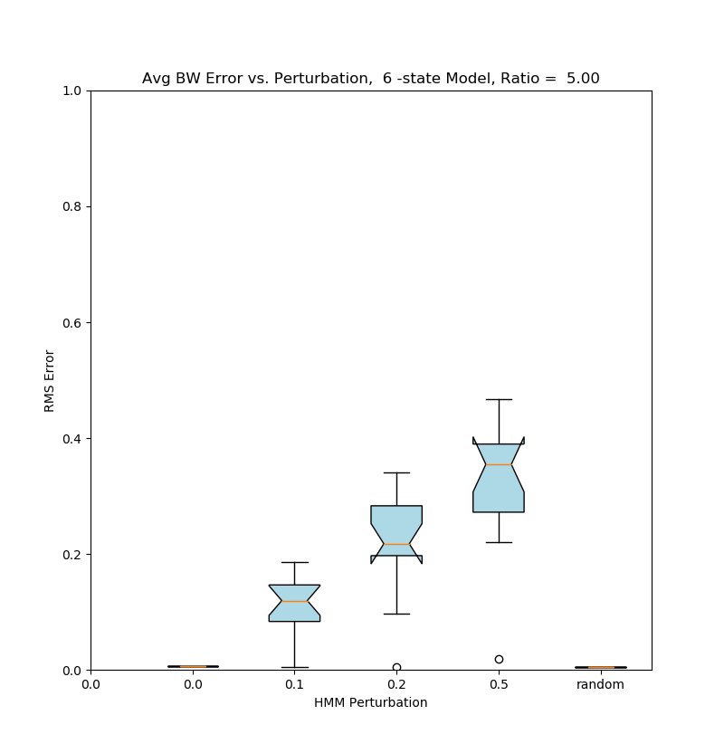
Parameter identification using the Baum-Welch algorithm (blue box plots of Figure 6) was a strong function of the perturbation away from the reference model for all values of $R$. As expected, the BW algorithm did not change the model if it was initialized with the exact reference value (perturbation = 0). A random initialization gave highly variable results but it should be noted that the RMS error measure only compared $A_{i,j}$ elements which are non-zero in the reference model. Thus the adapted randomized $A_{i,j}$ matrix could still be expected to be very different.

6 State Model

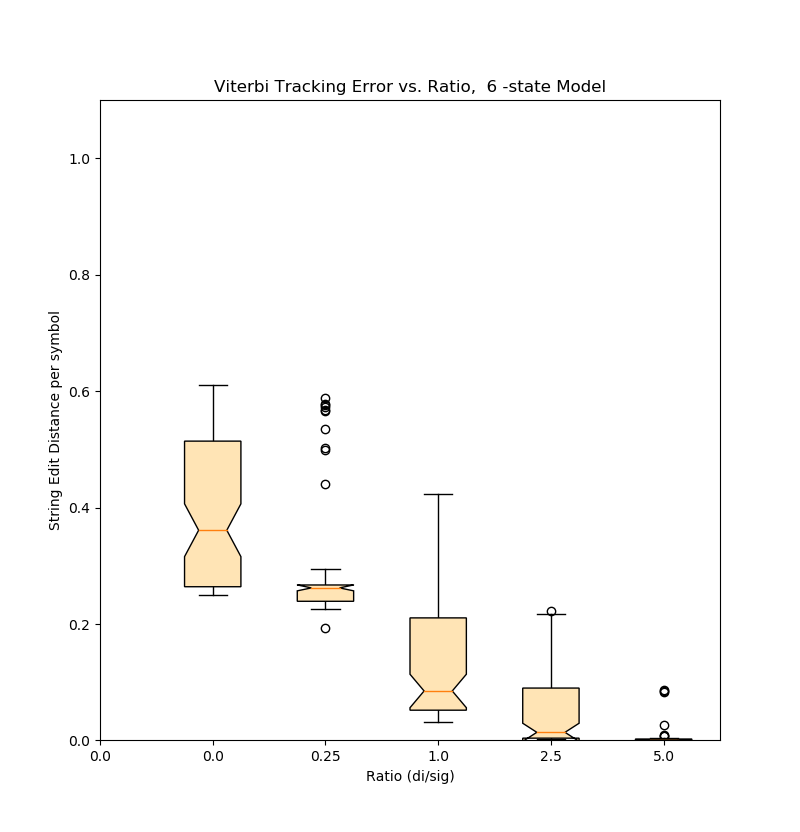
Performance of the Viterbi state tracking algorithm on the 6-state model and its dependence on the Ratio and perturbation parameters was qualitatively similar to that of the 16-state model, but errors were lower overall and relatively independent of perturbation.

Figure 8: Viterbi Algorithm state tracking error (SED) vs. Ratio (Left) and vs. Perturbation (Center). Graph details are same as Figure 7 The 6-state model has 12/36 non-zero elements.

5.4 Baum-Welch Parameter Identification

Finally, the hmmlearn Baum-Welch algorithm (HMM.fit()) was applied to the simulation-generated evolution file to test the ability to identify HMM parameters from data. In some of our experiments, we initialized the HMMs to random values because many previous studies have used randomly initialized parameters.

Baum Welch parameter estimation was evaluated on 300 randomly generated ABT-derived HMMs. We evaluated BW performance primarily in terms of 1) RMS error between the HMM parameters used to generate data and the final HMM parameters identified by BW and 2) The log probability (“LogP”) of the model after BW adaptation as a function of parameters such as model size and the amount of perturbation of the A-matrix.

Figure 9: Performance of BW algorithm for 6-state ABT derived data set. Graph details are same as Figure 7. The 6-state model has 12/36 non-zero elements.

6-State Model

For the 6-state model (not shown), BW identification worked much the same way although improvement in parameter identification was greater for 2.5 and 5.0 ratios with the smaller model. Average RMS_error vs. perturbation was better for all ratios with the 6-state model compared to the 16 state model. For the 6-state model with obscured states ($R=0$) parameter estimation improved with respect to the 16-state model, especially for the random initialization. For the 16-state model with transparent states ($R=5$) parameter estimation was better.

In both small and large models, parameter estimation error was minimal with transparent states. This is expected because the state transitions are unambiguous for those models.

6 Discussion and Future Work

Relation between BT and HMM

In this paper we have elucidated a relationship (to our knowledge new) between Behavior Trees and HMMs such that if the BT is augmented with probabilistic information, it then corresponds to a unique HMM. HMMs have been extremely successful in intelligent processing of time series data in fields such as speech, robotics and surgical manipulation. The anticipated applications for this result include processing and analysis of time series data, corrupted by noise or stochasticity, but arising from a process which can be described by a BT. Such processes include both autonomous agents and humans performing tasks with real-world interaction.

In such an application, this method could be applied as follows: 1) model the process with a BT according to expert knowledge 2) collect experimental data and manually label it with BT state (i.e label each observation symbol with the corresponding process step). Such labeling can be done by process experts or crowd sourced workers with or without information not present in the observation such as video or direct observation. 3) compute ABT statistics from the labeled data including $A_{i,j}$ and $B_{ij}$. 4) evaluate decoding/identification feasibility with divergence measures. 5) generate a HMM from the ABT 6) conduct the required data analysis using existing HMM algorithms.

In this paper, the emission probability density of each leaf was independent of the Success or Failure outcome. It may be that a modification in which the emission density for each state is conditioned on the two outcomes of each state would be more realistic in some applications.

Divergence measures.

We computed divergence measures for sets of artificial $B_{ij}$ distributions having different degrees of overlaps: an admittedly simplistic discrete Gaussian probability distribution. In an application, the divergence measures will be used to predict the effectiveness of using the methods of this paper on a new data set. Using the labeled data set (steps 2,3 above), we can compute the preferred divergence measure from the estimated $B_{ij}$. The empirical divergence measure thus obtained, along with Table 1, can relate a new data set to the experimental results in (Figure 6).

Viterbi state sequence decoding

The Viterbi algorithm worked well for most conditions (Figure 6 yellow box plots), especially when Ratio was greater than 1.0 ($JSD\approx 1.0$). With high divergence (“decodability”), decoding was perfect even with substantial difference between generative and decoding model parameters.

Baum-Welch parameter identification

Performance of BW parameter identification was more mixed (Figure 7 blue box plots). Results show that error in the HMM parameters was proportional to the difference between data generation and decoding models. For comparison, RMS error due to the model perturbation was about 0.1 compared to the 0.2-0.6 seen after BW convergence. This was true even for models with high divergence.

Implications for future work

Linking BTs to HMMs allows classic HMM algorithsm to be used as probabilitic tools for systems which can be modeled by BTs. Since HMMs in turn are linked to Dynamic Bayesian Networks (DBNs), an even wider set of tools are potentially available. In particular, this may improve model identification as some DBN techniques show better performance than Baum-Welch under certain conditions [8, 31].

Acknowledgments

The author would like to thank Shao-An (Sean) Yin for suggesting divergence measures and acknowlege support from NSF Grant IIS-1637444, and the University of Washington / Tsinghua University Global Innovation Exchange, GIX

References

- [1] Biing-Hwang Juang and Lawrence Rabiner. Mixture autoregressive hidden markov models for speech signals. IEEE Transactions on Acoustics, Speech, and Signal Processing, 33(6):1404–1413, 1985.
- [2] Biing-Hwang Juang and Laurence R Rabiner. Hidden markov models for speech recognition. Technometrics, 33(3):251–272, 1991.
- [3] Carol E Reiley, Henry C Lin, David D Yuh, and Gregory D Hager. Review of methods for objective surgical skill evaluation. Surgical endoscopy, 25(2):356–366, 2011.
- [4] Pierre Baldi, Yves Chauvin, Tim Hunkapiller, and Marcella A McClure. Hidden markov models of biological primary sequence information. Proceedings of the National Academy of Sciences, 91(3):1059–1063, 1994.
- [5] Chris Paxton, Andrew Hundt, Felix Jonathan, Kelleher Guerin, and Gregory D Hager. Costar: Instructing collaborative robots with behavior trees and vision. In Robotics and Automation (ICRA), 2017 IEEE International Conference on, pages 564–571. IEEE, 2017.
- [6] M. Colledanchise and Petter Ögren. How Behavior Trees Modularize Hybrid Control Systems and Generalize Sequential Behavior Compositions, the Subsumption Architecture, and Decision Trees. IEEE Transactions on Robotics, 33(2):372–389, April 2017.
- [7] Blake Hannaford, Randall A. Bly, Ian Humphreys, and Mark Whipple. Behavior trees as a representation for medical procedures. ArXiv, 1808.08954(1801.07864), January 2018.
- [8] Zoubin Ghahramani. An introduction to hidden markov models and bayesian networks. In Hidden Markov models: applications in computer vision, pages 9–41. World Scientific, 2001.
- [9] Lawrence R Rabiner. A tutorial on hidden markov models and selected applications in speech recognition. Proceedings of the IEEE, 77(2):257–286, 1989.
- [10] B. Hannaford and P. Lee. Hidden markov model analysis of force/torque information in telemanipulation. In Proceedings 1st International Symposium on Experimental Robotics, Montreal, June 1989.
- [11] B. Hannaford and P. Lee. Hidden markov model of force torque information in telemanipulation. International Journal of Robotics Research, 10(5):528–539, 1991.
- [12] Jie Yang, Yangsheng Xu, and Chiou S Chen. Hidden markov model approach to skill learning and its application to telerobotics. IEEE transactions on robotics and automation, 10(5):621–631, 1994.
- [13] Geir E Hovland, Pavan Sikka, and Brenan J McCarragher. Skill acquisition from human demonstration using a hidden markov model. In Robotics and Automation, 1996. Proceedings., 1996 IEEE International Conference on, volume 3, pages 2706–2711. Ieee, 1996.
- [14] J. Rosen, J.D. Brown, L. Chang, M. Sinanan, and B. Hannaford. Generalized approach for modeling minimally invasive surgery as a stochastic process using a discrete markov model. IEEE Transactions on Biomedical Engineering, 53(3):399–413, March 2006.
- [15] T.M. Kowalewski, J. Rosen, L. Chang, M. Sinanan, and B. Hannaford. Optimization of a vector quantization codebook for objective evaluation of surgical skill. In Proc. Medicine Meets Virtual Reality 12, pages 174–179, January 2004.
- [16] Damián Isla. Building a better battle: The halo 3 ai objectives system. http://web.cs.wpi.edu/~rich/courses/imgd4000-d09/lectures/halo3.pdf.
- [17] Chong-U Lim, Robin Baumgarten, and Simon Colton. Evolving behaviour trees for the commercial game defcon. In European Conference on the Applications of Evolutionary Computation, pages 100–110. Springer, 2010.
- [18] Danying Hu, Yuanzheng Gong, Blake Hannaford, and Eric J Seibel. Semi-autonomous simulated brain tumor ablation with ravenii surgical robot using behavior tree. In 2015 IEEE International Conference on Robotics and Automation (ICRA), pages 3868–3875. IEEE, 2015.
- [19] Danying Hu, Yuanzheng Gong, Blake Hannaford, and Eric J. Seibel. Path planning for semi-automated simulated robotic neurosurgery. In 2015 IEEE/RSJ International Conference on Intelligent Robots and Systems (IROS), September 2015.
- [20] P Kazanzides, J Zuhars, B Mittelstadt, B Williamson, P Cain, F Smith, L Rose, and B Musits. Architecture of a surgical robot. In Systems, Man and Cybernetics, 1992., IEEE International Conference on, pages 1624–1629. IEEE, 1992.
- [21] Petter Ogren. Increasing modularity of uav control systems using computer game behavior trees. In AIAA Guidance, Navigation and Control Conference, Minneapolis, MN, 2012.
- [22] Jana Tumova, Alejandro Marzinotto, Dimos V Dimarogonas, and Danica Kragic. Maximally satisfying ltl action planning. In Intelligent Robots and Systems (IROS 2014), 2014 IEEE/RSJ International Conference on, pages 1503–1510. IEEE, 2014.
- [23] Michele Colledanchise and Petter Ögren. How behavior trees modularize robustness and safety in hybrid systems. In Intelligent Robots and Systems (IROS 2014), 2014 IEEE/RSJ International Conference on, pages 1482–1488. IEEE, 2014.
- [24] Michele Colledanchise, Richard M Murray, and Petter Ögren. Synthesis of correct-by-construction behavior trees. In Intelligent Robots and Systems (IROS 2017), 2014 IEEE/RSJ International Conference on. IEEE, 2017.
- [25] M. Quigley, K. Conley, B. Gerkey, J. Faust, T. Foote, J. Leibs, R. Wheeler, and A.Y. Ng. Ros: an open-source robot operating system. In ICRA Workshop on Open Source Software, volume 3, 2009.
- [26] Alejandro Marzinotto, Michele Colledanchise, Christian Smith, and Petter Ögren. Towards a unified behavior trees framework for robot control. In Robotics and Automation (ICRA), 2014 IEEE International Conference on, pages 5420–5427. IEEE, 2014.
- [27] Michele Colledanchise, Alejandro Marzinotto, and Petter Ögren. Performance analysis of stochastic behavior trees. In 2014 IEEE International Conference on Robotics and Automation (ICRA), pages 3265–3272. IEEE, 2014.
- [28] J Andrew Bagnell, Felipe Cavalcanti, Lei Cui, Thomas Galluzzo, Martial Hebert, Moslem Kazemi, Matthew Klingensmith, Jacqueline Libby, Tian Yu Liu, and Nancy Pollard. An integrated system for autonomous robotics manipulation. In Intelligent Robots and Systems (IROS), 2012 IEEE/RSJ International Conference on, pages 2955–2962. IEEE, 2012.
- [29] accessed 2018.
- [30] Vladimir I Levenshtein. Binary codes capable of correcting deletions, insertions, and reversals. Soviet physics doklady, 10:707–710, 1966.
- [31] Raffay Hamid, Yan Huang, and Irfan Essa. Argmode-activity recognition using graphical models. In 2003 Conference on Computer Vision and Pattern Recognition Workshop, volume 4, pages 38–38. IEEE, 2003.