For a particular case of three-body scattering in two dimensions, and matching analytical expressions at a transition point, we obtain accurate solutions for the hyperspherical adiabatic basis and potential. We find analytical expressions for the respective, asymptotic, inverse logarithmic and inverse power potential behaviours, that arise as functions of the radial coordinate. The model that we consider is that of two particles interacting with a repulsive step potential, a third particle acting as a spectator. The model is simple but gives insight, as the 2-body interaction is long ranged in hyperspherical coordinates. The fully interacting 3-body problem is known, numerically, to yield similar behaviours that we can now begin to understand. That, clearly, is the ultimate aim.

Introduction

In a previous paper [1], the authors showed how, starting from hyperspherical harmonic expansions, they obtained adiabatic potentials, suitable for the calculations of three-body phase shifts at low energies. They constructed matrices consisting of hyperspherical harmonic matrix elements of the potential, together with centrifugal terms. The matrices were then diagonalized, to yield the desired adiabatic potentials. The calculations were for 3 particles in a plane, subject to finite repulsive core interactions.

The calculations were meant to establish a method which would lead to the evaluation, at low temperature, of a third fugacity coefficient in Statistical Mechanics. The latter task was subsequently carried out by Jei Zhen and one of the authors [2]. In both investigations, it was important to consider different cases, corresponding to the distinct representations of the permutation group and different physical situations, with either the 3 particles interacting or simply two of them interacting, with the third acting as a spectator.

Absolutely crucial, in these investigations, is the large-$\rho$ behaviour of the effective potentials (the adiabatic eigenvalue minus the appropriate centrifugal term). The nature of the long “tail” of the effective potential determines how the correspondent eigenphase shift behaves, as the energy tends to zero. Thus, our most significant result was that for the 3 most important types of the phase shifts, associated with the cases of ${}^{0}\Gamma_{1g}$, ${}^{0}\Gamma_{2g}$ and $\overline{\delta}$, the effective potentials behave as $1/(\rho^{2}\ln\rho)$, for large values of $\rho$, instead of the $1/\rho^{2}$ of the hyperspherical potential matrix elements. [The potential matrix elements are polynomials in $1/\rho^{2}$.] This then implies that the phase shifts, instead of tending to constants as the energy goes to zero, behave as $1/(\ln\,q)$, and therefore go to zero! (The variables $\rho$ and $q$ are, respectively, the hyper radius and the reduced wave number.) Other phase shifts were found to go to zero more powerfully. We show in Fig. 1 an example of the behaviour of the effective potential in the case ${}^{0}\Gamma_{1g}$ .

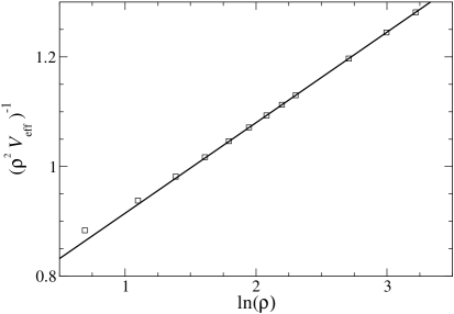
Figure 1: This figure shows the logarithmic behaviour for $\rho$ large of the effective potential, as a function of $\rho$, $\rho$ being the hyperradius, in the symmetry ${}^{0}\Gamma_{1g}$. Both, the calculated data (square symbols) and a fitting to the data (straight line), were taken from [2]

Though, in our old paper, our basic material was numerical, we were able nevertheless to propose “heuristic” formulae, to characterize the asymptotic behaviour of the $3$ types of eigenpotentials, of the remodelling that takes place to yield a different scattering from the one expected from the solution of a finite number of hyperspherical equations.

In this paper, we show that in one of the three cases mentioned above, the case $\overline{\delta}$, we succeed in calculating accurately the adiabatic eigenvectors and eigenvalues for all the values of $\rho$, and present analytical expressions valid in the asymptotic region.

While this calculation involves a case where only two of the particles interact, while the 3rd particle acts as a spectator, it is well to note that in the hyperspherical coordinate system the two-body interaction is long ranged (in $\rho$) and also that in the full hyperspherical calculations of the other cases, we only need, using symmetry and enforcing a restriction on the quantum numbers, to take into account the matrix element of one of the pair potentials.

Here, then, our calculations allow us to re-examine our previous results, and confirm and extend the asymptotic forms (and coefficients) that can be used to characterize the long range behaviour of the various effective potentials.

The KL Hyperspherical Coordinate System

The Harmonic Basis

For a system of three equal mass particles in two dimensions, we define the Jacobi coordinates

$$\vec{\eta}=(\vec{r}_{1}-\vec{r}_{2})/\sqrt{2}\hskip 28.45274pt\mbox{and}\hskip 28.45274pt\vec{\xi}=\sqrt{2/3}\,\left(\frac{\vec{r}_{1}+\vec{r}_{2}}{2}-\vec{r}_{3}\right)\;,$$

which allows us to separate, in the Hamiltonian, the center of mass coordinates from those associated with the internal motion.

Kilpatrick and Larsen [3] then introduce hyperspherical coordinates, associated with the moment of inertia ellipsoid, of the $3$ particles, which allows them to disentangle permutations from rotations and obtain harmonics which are pure representations of both the permutation and the rotation group. Taking the $z$ axis normal to the plane of the masses, we write for the cartesian components of the Jacobi coordinates

$$\eta_{x} = \rho(\cos\vartheta\cos\varphi\cos\psi+\sin\vartheta\sin\varphi\sin\psi),$$

$$\eta_{y} = \rho(\cos\vartheta\cos\varphi\sin\psi-\sin\vartheta\sin\varphi\cos\psi),$$

$$\xi_{x} = \rho(\cos\vartheta\sin\varphi\cos\psi-\sin\vartheta\cos\varphi\sin\psi),$$

$$\xi_{y} = \rho(\cos\vartheta\sin\varphi\sin\psi+\sin\vartheta\cos\varphi\cos\psi),$$ (1)

in terms of the hyper radius $\rho$ and of the three angles $\vartheta$, $\varphi$ and $\psi$.

The harmonics, in their unsymmetrized form, are then

$$Y_{N}^{\nu\lambda}(\Omega)=N_{n}^{\alpha\beta}\Theta_{n}^{\alpha\beta}(x)e^{i\nu\varphi}e^{i\lambda\psi}\;,$$ (2)

where $x=\sin{2\vartheta}$ and

$$\Theta_{n}^{\alpha\beta}(x)=(1-x)^{\alpha/2}(1+x)^{\beta/2}P_{n}^{\alpha,\beta}(x)\ .$$ (3)

$P_{n}^{\alpha,\beta}(x)\;$ is a Jacobi polynomial, and the normalization constant is

$$N_{n}^{\alpha\beta}=\left\{\left(\frac{N+1}{2^{\alpha+\beta+1}}\right)\left(\begin{array}[]{c}n+\alpha+\beta\\ \alpha\end{array}\right)\left(\begin{array}[]{c}n+\alpha\\ \alpha\end{array}\right)^{-1}\right\}^{1/2}\;.$$

The hyper radius $\rho\;$ satisfies $\rho^{2}=\eta^{2}+\xi^{2}$ and the angular components have the ranges

$$-1\leq x\leq 1,\hskip 28.45274pt-\pi/2\leq\varphi\leq\pi/2,\hskip 28.45274pt0\leq\psi\leq 2\pi\;.$$

Finally we have for the indices the relations

$$n=\frac{1}{2}[N-\mbox{{\rm max}}\{|\nu|,|\lambda|\}],\hskip 28.45274pt\alpha=\frac{1}{2}|\nu+\lambda|,\hskip 28.45274pt\beta=\frac{1}{2}|\nu-\lambda|\;,$$

where $N$ is the degree of the harmonic, and $\lambda$ is the inplane angular momentum quantum number. The indices $\nu$ and $\lambda$ take on the values $-N$ to $N$ in steps of $2$; all three have the same parity and $N=0,1,2,\ldots.$

Linear combinations of the basic harmonics can then be formed [3] to obtain irreducible bases, adapted to the symmetries of the physical problems [1, 2].

The Adiabatic Basis

For our model, the particles interact via a binary step potential

$$V(r_{ij})=\left\{\begin{array}[]{ll}V_{0},&r_{ij}\leq\sigma\\ 0,&r_{ij}>\sigma\end{array}\right.\hskip 28.45274pt$$ (4)

where the height $V_{0}$ and the range $\sigma$, are both finite.

In order for the $\lambda$ in the following equation, to be the same as that used by [1] and [2], we need to add a term $3/(4\rho^{2})$. That is because the angular part of the Laplacian has eigenvalues $-N(N+2)$ and not the $-[(N+1)^{2}-1/4]$ used in the coupled equations used by these authors.

The adiabatic eigenfunctions $B_{\ell}$ are then defined as satisfying

$$\left\{-\frac{1}{\rho^{2}}\nabla_{\Omega}^{2}+\frac{3}{4\rho^{2}}+\frac{2m}{\hbar^{2}}V(\rho,\Omega)\right\}B_{\ell}=\lambda_{\ell}(\rho)B_{\ell}\;,$$ (5)

where $V(\rho,\Omega)$ is either the sum of the binary potentials or, simply one of the binary potentials, say $V(r_{12})$, expressed as a function of $\rho$ and the angles. The index $\ell$ stands for the set of quantum numbers which characterize and index the particular class of solutions. $\lambda_{\ell}(\rho)$ is the eigenvalue, which upon subtraction of a “centrifugal” type term yields the effective potential, of concern to us later on.

The eigenfunctions may now be used to expand the wavefunctions of the physical systems:

$$\Psi=\sum_{\ell^{\prime}}B_{\ell^{\prime}}(\rho,\Omega)\phi_{\ell^{\prime}}(\rho)\;,$$ (6)

where the amplitudes $\phi_{\ell}(\rho)$ are the solutions of the coupled equations:

$$-\sum_{\ell^{\prime}}\int\!d\Omega\,B^{\ast}_{\ell}(\rho,\Omega)\frac{\partial^{2}}{\partial\rho^{2}}\left(B_{\ell^{\prime}}(\rho,\Omega)\phi_{\ell^{\prime}}(\rho)\right)+\lambda_{\ell}(\rho)\phi_{\ell}(\rho)=(2mE/\hbar^{2})\phi_{\ell}(\rho).$$ (7)

The adiabatic eigenfunctions can themselves be expanded in hyperspherical harmonics and this is how a large set of them were calculated in the papers quoted earlier. The symmetries of the hyperspherical harmonic basis are, of course, reflected in the solutions of the adiabatic eigenvectors. For the fully symmetric Hamiltonian, the set of solutions divides into six separate subsets [3], each requiring calculations involving combinations of matrix elements of only one of the binary potentials, but with restrictions on the quantum numbers of the unsymmetrized harmonics involved. In the case of two interacting particles, with a third as a spectator, we find an additional four subsets.

The numerical approach was then, for each $\rho$, to evaluate a large potential matrix, with the appropriate harmonic basis, add to this the (diagonal) “centrifugal” contribution arising from the angular part of the kinetic energy (the angular part of the Laplacian in the Hamiltonian) and diagonalize to obtain the required adiabatic eigenvalues. The number of harmonics, needed for numerical convergence, increases as a function of $\rho$, but it was our fortunate experience to find that it was possible to evaluate correctly the eigenvalues, that we sought, for values of $\rho$ large enough that the behaviour of $\lambda_{\ell}(\rho)$ could be described by asymptotic forms. We were able to characterize them, and this gave us the values of $\lambda_{\ell}(\rho)$ for all the larger values of $\rho$.

Dual Polar Set of Coordinates

The Harmonic Basis

In this part of the paper we wish, exclusively, to consider the case of two particles interacting together, the third acting as a spectator. As we shall show, we are then able to obtain exact adiabatic solutions.

Our reasoning is as follows. When the third particle does not interact with the other two, this must imply that the motion of the pair (1,2), and therefore its angular momentum, is unaffected by the motion of the third particle. In a parallel fashion, the motion of the third particle, and its angular momentum about the center of mass of the particles (1,2), must be a constant as well. If we choose our coordinates carefully, the angular behaviour of two of the angles should “factor” out and, for a given $\rho$, only one variable should be involved in a key differential equation.

We note that in the KL coordinates, the distances between particles involve two of the angles, for example $r_{12}^{2}$ equals $\rho^{2}(1+\cos 2\vartheta\cos 2\varphi)$. To get around this, we choose an angle to give us the ratio of the length of the $2$ Jacobi vectors, and then polar coordinates for each of them. Thus, we represent $\Omega$ by $(\theta_{1},\theta_{2},\phi)$, where $\eta=\rho\cos\phi$, $\xi=\rho\sin\phi$ and $\eta_{x}=\eta\cos\theta_{1}$, $\eta_{y}=\eta\sin\theta_{1}$, $\xi_{x}=\xi\cos\theta_{2}$, $\xi_{y}=\xi\sin\theta_{2}$. The ranges of these angles are

$$0\leq\phi\leq\pi/2,\hskip 28.45274pt0\leq\theta_{1}\leq 2\pi,\hskip 28.45274pt0\leq\theta_{2}\leq 2\pi\;.$$

To obtain the harmonics, in a manner which is suitable to also demonstrate the link with the KL harmonics, we introduce complex combinations of the Jacobi coordinates, i.e. the monomials

$$z_{1} = (\eta_{x}+\imath\eta_{y})$$

$$z^{*}_{1} = (\eta_{x}-\imath\eta_{y})$$

$$z_{2} = (\xi_{x}+\imath\xi_{y})$$

$$z^{*}_{2} = (\xi_{x}-\imath\xi_{y})$$ (8)

It then follows that

$$\rho^{2} = (z_{1}z^{*}_{1}+z_{2}z^{*}_{2})$$

$$\nabla^{2} = 4\,\left(\frac{\partial^{2}}{\partial z_{1}\partial z^{*}_{1}}+\frac{\partial^{2}}{\partial z_{2}\partial z^{*}_{2}}\right),$$ (9)

and, clearly, $z_{1}$, $z^{*}_{1}$, $z_{2}$ and $z^{*}_{2}$ each satisfies Laplace’s equation, as do the combinations $z_{1}z_{2}$, $z_{1}z^{*}_{2}$, $z^{*}_{1}z_{2}$, $z^{*}_{1}z^{*}_{2}$ and these combinations raised to integer powers.

Writing $\rho_{1}^{2}=z_{1}z^{*}_{1}$ and $\rho_{2}^{2}=z_{2}z^{*}_{2}$, we can write as the most general solution arising from the monomials $z_{1}$ and $z_{2}$:

$$z_{1}^{\ell_{1}}z_{2}^{\ell_{2}}P_{\ell}^{\ell_{2},\ell_{1}}\left(\frac{\rho_{2}^{2}-\rho_{1}^{2}}{\rho_{2}^{2}+\rho_{1}^{2}}\right)(\rho_{1}^{2}+\rho_{2}^{2})^{\ell}\,,$$

where $\ell_{1}$, $\ell_{2}$ and $\ell$ are positive integers or zero, and $P_{\ell}^{\ell_{2},\ell_{1}}$ is a Jacobi polynomial.
In terms of the angles, our expression becomes proportional to:

$$\rho^{\ell_{1}+\ell_{2}+2\ell}(\cos^{2}\phi)^{\ell_{1}/2}(\sin^{2}\phi)^{\ell_{2}/2}P_{\ell}^{\ell_{2},\ell_{1}}(\cos 2\phi)e^{\imath\theta_{1}\ell_{1}}e^{\imath\theta_{2}\ell_{2}}\,,$$

and, finally, in terms of $z$ equal to $\cos 2\phi$, we define our unnormalized harmonic:

$$Y_{\ell}^{\ell_{1},\ell_{2}}(\theta_{1},\theta_{2},z)=(1+z)^{|\ell_{1}|/2}(1-z)^{|\ell_{2}|/2}\,P_{\ell}^{|\ell_{2}|,|\ell_{1}|}(z)\,e^{\imath\theta_{1}\ell_{1}}e^{\imath\theta_{2}\ell_{2}}\,,$$ (10)

where now $\ell_{1}$ and $\ell_{2}$ can be positive, negative, integers - or zero. (This takes into account the other combinations $z_{1}z_{2}^{*}$, etc.) The order of the harmonic is $N$ equal to $|\ell_{1}|+|\ell_{2}|+2\ell$.

The Adiabatic Differential Equation

Writing

$$\nabla_{\eta}^{2}+\nabla_{\xi}^{2}=\left(\,\frac{\partial^{2}}{\partial\rho^{2}}+\frac{3}{\rho}\frac{\partial}{\partial\rho}\,\right)+\frac{1}{\rho^{2}}\nabla_{\Omega}^{2}\,,$$ (11)

inserting our polar coordinates into the left hand side and changing to our variable $z$, we find:

$$\nabla_{\Omega}^{2}=4(1-z^{2})\frac{\partial^{2}}{\partial z^{2}}-8z\frac{\partial}{\partial z}+\frac{2}{(1+z)}\frac{\partial^{2}}{\partial\theta_{1}^{2}}+\frac{2}{(1-z)}\frac{\partial^{2}}{\partial\theta_{2}^{2}}\,\,.$$ (12)

If we now write our adiabatic eigenfunctions as

$$B_{N}^{\ell_{1}\ell_{2}}(\rho,\Omega)=e^{i\ell_{1}\theta_{1}}e^{i\ell_{2}\theta_{2}}\,(1+z)^{|\ell_{1}|/2}(1-z)^{|\ell_{2}|/2}\,F_{\ell}^{|\ell_{1}|,|\ell_{2}|}(\rho,z)\;,$$ (13)

then the functions $F$ will satisfy the equation:

$$\left[-4(1-z^{2})\frac{\partial^{2}}{\partial z^{2}}+4((2+\ell_{1}+\ell_{2})z+\ell_{2}-\ell_{1})\frac{\partial}{\partial z}\right]F_{\ell}^{\ell_{1},\ell_{2}}(\rho,z)$$ (14)

$$+ \left[(\ell_{1}+\ell_{2})(\ell_{1}+\ell_{2}+2)+\frac{3}{4}+\rho^{2}\overline{V}(\rho,z)\right]\ \ F_{\ell}^{\ell_{1},\ell_{2}}(\rho,z)=\rho^{2}\lambda(\rho)F_{\ell}^{\ell_{1},\ell_{2}}(\rho,z)$$

where $\overline{V}(\rho,z)$ equals $2m/\hbar^{2}$ times the potential and in our notation we have dropped the absolute value indications. All the indices will be understood to be positive or zero.

When $\overline{V}(\rho,z)=0$, we can obtain a solution which is analytic between $-1\leq z\leq+1$. For $\lambda$ equal to $(\ell_{1}+\ell_{2}+2\ell)(\ell_{1}+\ell_{2}+2\ell+2)/\rho^{2}$ and $\ell$ a non-negative integer, we find that our $F$ is simply $P_{\ell}^{\ell_{2},\ell_{1}}(z)$, the Jacobi polynomial which appears in our Eq. (10). The $N$ that appears in the $B$ of Eq. (13) is the order of the corresponding harmonic.
We now scale our $\rho$. I.e., we let our new $\rho$ equal our old $\rho/\sigma$. Then, for $\rho>\frac{1}{\sqrt{2}}$ and our new potential

$$\overline{V}(\rho,z)=\left\{\begin{array}[]{ll}(2m/\hbar^{2})V_{0}\,\sigma^{2}&-1\leq z\leq-1+1/\rho^{2}\\ 0&-1+1/\rho^{2}<z\leq 1\;,\end{array}\right.$$ (15)

the solutions of this equation, which behave reasonably at $z$ equal to $-1$ and $+1$, will be seen to be proportional to extensions of the Jacobi polynomials to functions with non-integer indices, in a relationship similar to that of Legendre polynomials and Legendre functions. To motivate and clarify our procedure we first consider the case of $\ell_{1}=\ell_{2}=0$, with and without potential.

When the potential is put to zero and we factor a $4$ as well as change the sign, the differential equation reads

$$\left[(1-z^{2})\frac{\partial^{2}}{\partial z^{2}}-2z\frac{\partial}{\partial z}+\ell\,(\ell+1)\right]\;F_{\ell}^{0,0}(\rho,z)=0.$$ (16)

This is, of course, the Legendre differential equation and, with $\ell$ a positive or zero integer, the well behaved solutions are the Legendre polynomials.

In the case of our potential, which is zero or a constant (only a function of $\rho$) in the different ranges of $z$, we can write our differential equation in a very similar form, i.e. as

$$\left[(1-z^{2})\frac{\partial^{2}}{\partial z^{2}}-2z\frac{\partial}{\partial z}+\nu\,(\nu+1)\right]\;F_{\nu}^{0,0}(\rho,z)=0\,,$$ (17)

where for $-1+1/\rho^{2}<z\leq 1$

$$\nu\,(\nu+1)=\rho^{2}\,\lambda\,(\rho)/4-\frac{3}{16}$$ (18)

and  for $-1\leq z\leq-1+1/\rho^{2}$

$$\nu\,(\nu+1)=\rho^{2}\,[\lambda\,(\rho)-\overline{V}_{0}]/4-\frac{3}{16}\;.$$ (19)

Denoting the respective values of $\nu$ as $\nu_{1}$ and $\nu_{2}$, the corresponding solutions are the Legendre function $P_{\nu_{1}}(z)$ and the combination

$$P_{\nu_{2}}(-z)=\cos(\pi\nu_{2})\,P_{\nu_{2}}(z)-(2/\pi)\,\sin(\pi\nu_{2})\,Q_{\nu_{2}}(z)\,,$$

of the first and second Legendre functions.

The point is as follows. Whereas $P_{\nu_{1}}(z)$ is well behaved at $z$ equal to $1$, and is suitable as a solution for its range in $z$ from $-1+1/\rho^{2}$ to $1$, both the $P_{\nu_{2}}(z)$ and $Q_{\nu_{2}}(z)$ have a logarithmic singularity at $z$ equals $-1$. The combination that we propose, however, is such that the logarithmic terms cancel out and the combination [4] is a well behaved solution in the range $-1$ to $-1+1/\rho^{2}$.

Expressing these solutions as power series, the first about $z$ = $1$, the second about $z$ = $-1$, we obtain

$${}_{2}F_{1}(-\nu_{1},\nu_{1}+1;1;\frac{1}{2}(1-z)), \mbox{for}-1+1/\rho^{2}<z\leq 1$$

and (20)

$${}_{2}F_{1}(-\nu_{2},\nu_{2}+1;1;\frac{1}{2}(1+z)), \mbox{for}-1\leq z\leq-1+1/\rho^{2}$$

Our overall solutions are then obtained by matching the logarithmic derivative of the two solutions (above) at the boundary: at $z$ equal $-1+1/\rho^{2}$. This then also yields the adiabatic eigenvalues.

It now remains to note that for the cases of $\ell_{1}$ and $\ell_{2}$ not equal to zero, we can use the same procedure. We have, for the two regimes, solutions proportional to

$${\rm(R)} {}_{2}F_{1}(-\nu_{1},\nu_{1}+|\ell_{1}|+|\ell_{2}|+1;|\ell_{2}|+1;\frac{1}{2}(1-z)), \mbox{for}-1+1/\rho^{2}<z\leq 1$$

and

$$(\mathrm{L}) {}_{2}F_{1}(-\nu_{2},\nu_{2}+|\ell_{1}|+|\ell_{2}|+1;|\ell_{1}|+1;\frac{1}{2}(1+z)), \mbox{for}-1\leq z\leq-1+1/\rho^{2}$$ (22)

henceforth labelled Right $\left(R\right)$ and Left $\left(L\right)$.

For each choice of $\ell_{1}$ and $\ell_{2}$ there is an infinite set of values of $\nu_{1}\;$ for which the logarithmic derivative of the hypergeometrical functions can be matched at $z$ equal to $-1+1/\rho^{2}$. For each such value of $\nu_{1}$, the adiabatic eigenvalue is then given by

$$\lambda(\rho)=\frac{(2\nu_{1}+|\ell_{1}|+|\ell_{2}|+1)^{2}-\frac{1}{4}}{\rho^{2}}\;.$$ (23)

When $V_{0}=0$, the adiabatic basis reduces to the hyperspherical harmonic basis of Eq. (10), since the hypergeometrical functions reduce to Jacobi polynomials, and $\nu_{1}\equiv\nu_{2}=\ell$. So our $B_{N}^{\ell_{1},\ell_{2}}$ is precisely the $Y_{\ell}^{\ell_{1},\ell_{2}}(\theta_{1},\theta_{2},z)$.

Comparison of the Adiabatic Eigenvalues

First a historical note.

The results obtained by diagonalizing matrices to obtain the adiabatic potentials, and shown here below in this section, were drawn from reference [5]. The ‘direct’ results are obtained by solving numerically Eq. (14), matching the logarithmic derivatives of the appropriate analytical solutions, at the edge of the binary potential.

When the numerical work was done (using the KL basis), lists were made of the appropriate harmonics needed to form the matrices (potential and centrifugal) which, when added and diagonalized, yield the adiabatic eigenvalues. We now need to identify these eigenvalues and compare them with those obtained by the new method. This is not trivial, but an immediate remark can be made.

First of all, in both approaches the angular momentum $\lambda$ is a good quantum number. Further, in the new basis, we can write:

$$\lambda=\ell_{1}+\ell_{2}\;.$$ (24)

This follows from the fact that $\ell_{1}$ specifies the angular momentum of the 1-2 pair and $\ell_{2}$ specifies the angular momentum of the third particle relative to the center of mass of the first two. Thus their sum defines the total inplane angular momentum. Hence, for example, when $\lambda=0$ we can have all pairs $\ell_{1}$ and $\ell_{2}$ with $\ell_{1}=-\ell_{2}$. If $\ell_{1}=\ell_{2}=0$, this then provides a single eigenvalue for each choice of $N=2\,\ell,\,\ell=0,1,2,\ldots.$

Another indicator is whether $n$ is even or odd, which is very significant in the drawing up of the lists, associated with the symmetries of the harmonics. Proceeding, then, we compare values of the effective potential, defined by

$$V_{{\rm eff}}(\rho,N)=\lambda(\rho)-\frac{(N+1)^{2}-\frac{1}{4}}{\rho^{2}}\;,$$ (25)

where we subtract from each eigenvalue the value of the centrifugal term that would correspond to it, if the binary potential were allowed to go to zero. These have been extensively tabulated by Zhen [5], but see also [1, 2].

In Table 1 we confirm a central result of the previous authors’ work. We demonstrate the convergence of the truncated matrix method to the result obtained directly. This, for the simplest case, $N=0$ and, a sample value of $\rho=5\;$ and $\Lambda^{*}=10$. ($\Lambda^{*}=(h^{2}/mV_{0}\sigma^{2})^{1/2}$). As we see, the result is excellent.

$N_{{\rm max}}$	$V_{{\rm eff}}(5,0)$
$110$	$0.011754744$
$120$	$0.011754730$
$130$	$0.011754670$
$140$	$0.011754666$
Direct	$0.011754562$

Table 1: Convergence of the matrix method

A more extensive set of comparisons is made in Table 2, where selected values of the effective potential, obtained from eigenvalues of the truncated matrix, are chosen for various values of $N$, $\lambda$ and $n$ and compared with the direct results. In all cases, except the first, the matrix was truncated at $N_{{\rm max}}=100$, where $N_{{\rm max}}$ is the maximal order of the hyperspherical elements used in constructing the matrix.

$V_{{\rm eff}}(\rho,N)$
Truncated Matrix				Direct
$n$	$\lambda$	$N$	$V_{{\rm eff}}(5,N)$	$\ell$	$|\ell_{1}|$	$|\ell_{2}|$	$V_{{\rm eff}}(5,N)$
E	0	0	0.011754666	0	0	0	0.011754562
E	0	2	0.037577818	1	0	0	0.037577462
O	0	2	0.000874927	0	1	1	0.000874911
E	0	4	0.062609805	2	0	0	0.062609219
E	0	4	0.00005971	0	2	2	0.00005971
O	2	4	0.00413519	1	1	1	0.00413512
E	1	1	0.024168	0	0	1	0.02416738
E	1	1	0.00029592	0	1	0	0.00029591
O	1	3	0.000024	0	2	1	0.00002426
O	1	3	0.00172537	0	1	2	0.00172529
E	1	3	0.050462	1	0	1	0.0504588
E	1	3	0.00226748	1	1	0	0.00226737
E	2	2	0.00000616	0	2	0	0.00000616
O	2	2	0.036849	0	0	2	0.03684737
E	2	4	0.000088636	1	2	0	0.000088629
E	2	4	0.062866	1	0	2	0.06286247

Table 2: Some effective potential values in the $\overline{\delta}$ class

Here we must alert the reader. The above results were obtained without focusing on the permutational classifications. Some of these values belong to effective potentials which decay as inverse logarithms for large $\rho$, others will decay much faster, as we will see.

Asymptotic Behaviour

The matching of logarithmic derivatives provides a means of obtaining information about the asymptotic behaviour of the eigenvalues, and hence the effective potentials, as the hyper-radius, $\rho$, gets large. There is however a particular difficulty in finding this behaviour. It is that it is not simply a case of looking at the limiting behaviour of ${}_{2}F_{1}(a,b;c;\epsilon)$ and ${}_{2}F_{1}(a,b;c;1-\epsilon)$ as $\epsilon\rightarrow 0$, because the expressions corresponding to $a$ and $b$ both depend on $\rho$.

We recall that the effective potential, $V_{{\rm eff}}$, is obtained by matching, at the points $z=-1+\rho^{-2}$, the logarithmic derivatives of the functions (R) and (L) given in the expressions (The Adiabatic Differential Equation, 22), in conjunction with the Eqs. (1, 36) given in the Appendix.

Inverse logarithmic behaviour

In the analysis of the asymptotic behaviour of the adiabatic eigenvalues in the Appendix, we show that, in the case corresponding to $\ell_{1}=0$, the effective potential behaves as:

$$\rho^{2}V_{\mbox{eff}}(\rho)=\frac{1}{A+B\ln\rho}\;+\frac{1}{4(N+1)^{2}\left(A+B\ln\rho\right)^{2}}\,.$$ (26)

In this case $N$, the order of the harmonic, simplifies to $\left|\ell_{2}\right|+2\ell$ and the constants $A$ and $B$ are defined as

$$A=\frac{1}{4(N+1)}\left[\frac{2\,I_{0}\left(\sqrt{\frac{V_{0}}{2}}\right)}{{\sqrt{\frac{V_{0}}{2}}}\,I_{1}\left(\sqrt{\frac{V_{0}}{2}}\right)}-{\displaystyle\sum_{p=1}^{\ell}\frac{1}{p}}-{\displaystyle\sum_{p=1}^{\ell+\left|\ell_{2}\right|}\frac{1}{p}}+\ln 2\right]\,,\qquad\qquad B=\frac{1}{2(N+1)}\;.$$ (27)

The $I_{i}$’s are modified Bessel functions of integer order of the first kind, and it should be understood that $\sum_{1}^{0}\equiv 0$ .

Equation (26) yields our very best description of the asymptotic behaviour of $V_{{\rm eff}}$, being accurate for the highest values of $\rho$, as well as for a wide range of lower values. We refer to the potential of that description as $V_{{\rm best}}$.

Its leading term, together with the expressions for the constants (27), was previously found by Klemm and Larsen [6]. It properly describes $V_{{\rm eff}}$ for the upper range of values of $\rho$. We denote it as $V_{{\rm KL}}$. (Not to be confused with the $KL$ of the hyperspherical basis,)

A similar equation, giving an improved representation of the effective potential for lower values of $\rho$, can be found by incorporating part of the quadratic term into the simple inverse logarithmic relationship. We found as a result (see the Appendix):

$$\rho^{2}V_{\mbox{eff}}(\rho)\sim\frac{1}{A^{*}+B^{*}\ln\varrho},$$ (28)

where

$$A^{*}=A-\frac{1}{4(N+1)^{2}}\,,\qquad{\cal\qquad}B^{*}=B.$$ (29)

We refer to it as $V_{{\rm wider}}$, for the wider range of its description.

We emphasize that, in all 3 asymptotic expressions, the asymptotically dominant term in $1/(B\ln(\rho))$ always stays the same.

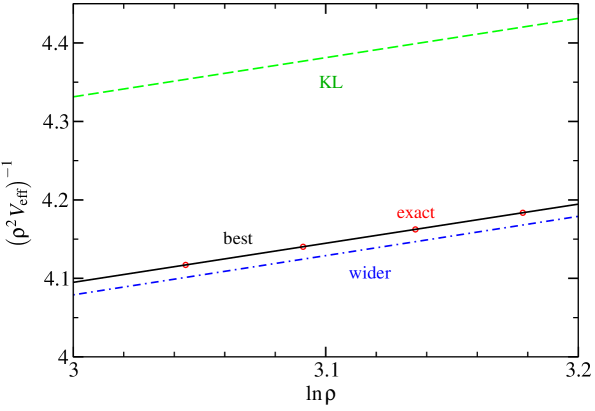
Figure 2: This figure shows the asymptotic behaviour of the effective potential as a function of the hyperradius, for $\ell=\ell_{1}=\ell_{2}=0$, and compares the different approximations explained in this paper. The red dots correspond to values of $V_{\rm exact}$, obtained by matching numerically the functions (The Adiabatic Differential Equation, 22); the black solid, to $V_{\rm best}$; the blue dot-dash line, to $V_{\rm wider}$ and the green dash line corresponds to $V_{\rm KL}$ [6]

In Figure (2), we present a comparison, in the $\rho$ large region, between the exact values of the effective potential (dots), $V_{{\rm exact}}$, with those obtained using the various asymptotic analytical expressions derived in the present paper. The case shown corresponds to the values of $\ell_{1}=0,\,\ell_{2}=0$ and $\ell=0$. The exact set of values was calculated numerically, by matching the logarithmic derivative of the solutions given in equation (20), at the point $z=-1+1/\rho^{-2}$. From the figure we can appreciate the inverse-logarithmic behaviour for the whole set of results, and that the exact results are very well described by the improved expression for the effective potential, $V_{{\rm best}}$.

At this point, we would like to introduce another table (Table 3).

In it, we display values of the constant $\cal{A}$, in fits obtained by Zhen [5] in her thesis work (and also published in [2]). They are fits of the numerical values of some of the dominant effective potentials, for $\rho\geq 15$. We join the comparable values of $A$ and $A^{*}$ of our analytic expressions.
(In her thesis, she also compares her $\cal B$’s with the postulated values of [1]; sometimes her fits include a ${\cal C}/\rho^{2}$ in the inverse logarithmic expression.)

$n$	$\lambda$	$N$	$\ell_{1}$	$\ell$	$\ell_{2}$	${\cal A}$ (Zhen)	$A$	$A^{*}$
$E$	0	0	0	0	0	2.6064	2.8293	2.5793
$E$	0	2	0	1	0	0.7581	0.7764	0.748659
$E$	0	4	0	2	0	0.4146	0.4159	0.4059
$E$	1	1	0	0	1	1.2381	1.2897	1.22715
$E$	1	3	0	1	1	0.5493	0.5511	0.5355
$E$	1	5	0	2	1	0.3356	0.3327	0.3257

Table 3: Comparison of numerical and analytic
asymptotic leading terms.

We must emphasize that the values for ${\cal A}$, and ${\cal B}$, that were obtained by Zhen, correctly fit her data. We obtain similar results, when restricting ourselves to intermediate values of large $\rho$.
Our asymptotic expressions, first, truly model the highest values of $\rho$, and then - with different degree of success - model the behaviour for smaller values of $\rho$.

Inverse $\rho$ behaviour

We found, in the cases $\ell_{1}\neq 0$, that the potentials have a different behaviour when $\rho$ is large. We show in the Appendix that the leading term of the potential for this case, in the asymptotic region, is

$$\rho^{2}V_{\mbox{eff}}(\rho)\simeq\frac{q}{\rho^{2\left|\ell_{1}\right|}}$$ (30)

where

$$\frac{1}{q}=\frac{2^{|\ell_{1}|-2}}{({N+1})C_{N-\ell}^{|\ell_{1}|}C_{|\ell_{1}|+\ell}^{|\ell_{1}|}}\left(\frac{1}{|\ell_{1}|}+\frac{{2}I_{|\ell_{1}|}\left(\sqrt{\frac{V_{0}}{2}}\right)}{\sqrt{{\frac{V_{0}}{2}}}\ I_{|\ell_{1}|+1}\left(\sqrt{\frac{V_{0}}{2}}\right)}\right),\ N=2\ell+|\ell_{1}|+|\ell_{2}|.$$ (31)

In figures (3a) and (3b) we exhibit this behaviour for the two cases, $\ell_{1}=1$ and $\ell_{1}=2$, respectively. In both examples $\ell_{2}=0$ and $\ell=0$. The figures show how the exact values of the potentials are approaching their asymptotic behaviours, as given by Eq. (30).

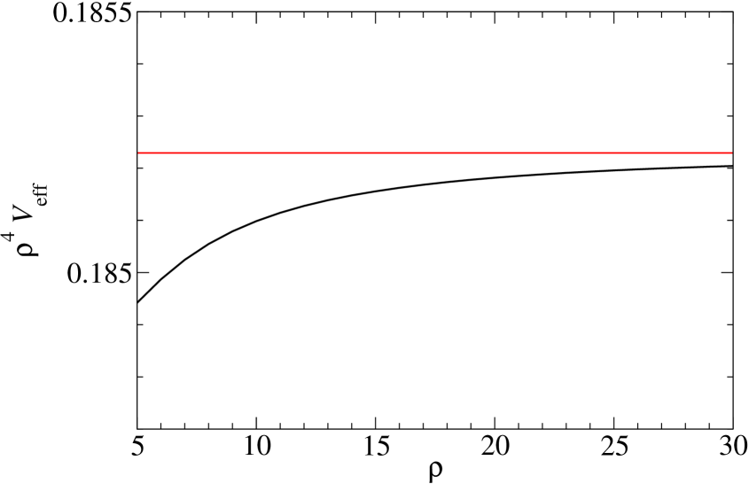
(a) This figure shows the effective potential $V_{{\rm exact}}$ (black curve) approaching its inverse-power asymptotic behaviour given by Eq. (30), as $\rho$ increases, for $\ell_{1}=1$ and $\ell_{2}=0=\ell$. From Eq. (31), $q=0.185229$ (straight red curve).

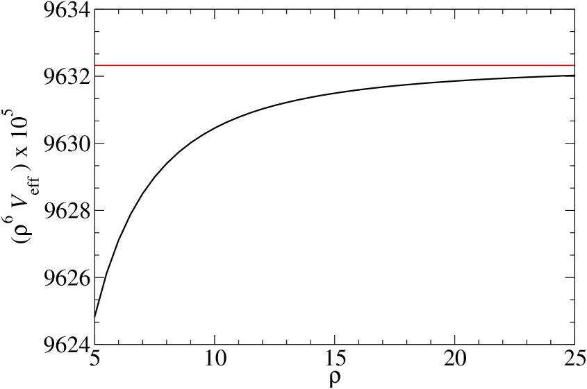
(b) This figure shows the exact effective potential $V_{{\rm exact}}$ (black curve) , for $\ell_{1}=2$ and $\ell_{2}=0=\ell$, approaching its inverse-power asymptotic behaviour given by Eq. (30), as $\rho$ increases. In this case, Eq. (31), gives a value for $q=0.096323$ (straight red curve).

Figure 3: Asymptotic effective potentials for $\ell_{1}$ not equal to zero.

Phase shifts

In reference [7] it is shown that when $V_{{\rm eff}}$ behaves as $1/(\rho^{2}{\cal B}\ln\rho)$, the long-range part of the potential dominates the behaviour of the phase shift, and the latter goes to zero when $k\rightarrow 0$ as

$$\delta\rightarrow\left(\frac{\pi}{4}\right)\,\frac{1}{{\cal B}\ln\,k}.$$ (32)

It is notable that this inverse logarithmic behaviour occurs when $\ell_{1}$ equals zero, not $\ell_{2}$. I.e., it is when the interacting pair, of particles, has zero angular momentum. We are then drawn to the 2-body problem, in 2 dimensions, of interacting hard discs, where we find, for zero angular momentum, precisely the same result.

Indeed, for hard discs, and a potential of radius $\sigma$, the wave function $\psi$, in terms of Bessel and Neumann functions, and for angular momentum $L$, reads:

$$\psi\propto N_{L}(k\sigma)J_{L}(kr)-J_{L}(k\sigma)N_{L}(kr)$$

and thus

$$\tan(\delta_{L}(k))=\frac{J_{L}(k\sigma)}{N_{L}(k\sigma)}$$

At low energies, we therefore find that for hard discs, as for our step functions, that $\delta_{0}(k)\rightarrow(\pi/2)(1/\ln k\sigma)$, and $\delta_{L}(k)\propto(k\sigma)^{2L}$, when $L\neq 0$. .

We now wish to address the case of $\ell_{1}\neq 0$.

For $\ell_{1}=0$, we have argued that the ‘tail’ of the effective potential dominates the small $k$ behaviour of the phase shift. We do so again when $\ell_{1}\neq 0$.

For a two-body problem with a radial potential that falls off as $r^{-s}$ for large $r$, Mott and Massey [8] obtain a behaviour for the phase shift $\eta_{L}$ ,at low energies, of the form

$${\displaystyle\lim_{k\rightarrow 0}\,k^{s-2}\,\cot\,\delta_{L}={\rm constant,}}$$

when the angular momentum $L+\frac{1}{2}>(s-2)/2$. In our adiabatic hyperspherical approach, the role of $L+1/2$, in the two-body system, is played by $N+1$, and therefore the criterion for tail-dominant behaviour is that $N+1$ be greater than $\left(s-2\right)/2$. For $|\ell_{1}|$ in general (not zero), we see that the minimum value of $N$ is $|\ell_{1}|$, and that the value of $s$ equals $2|\ell_{1}|+2$. The inequality is always satisfied $(|\ell_{1}|+1)>|\ell_{1}|$ , and the tail always dominates.

As a result, we see that, given our asymptotic result of

$$\rho^{2}V_{\mbox{eff}}(\rho)\simeq\frac{q}{\rho^{2\left|\ell_{1}\right|}}$$ (33)

and the expression of Mott and Massey, our adiabatic phase shift result for $\ell_{1}$ is proportional to $(k\sigma)^{2|\ell_{1}|}$, and therefore in agreement with the hard disc result.

Symmetry considerations

As representations of the permutational groups, the case $\overline{\delta}$ divides into 4 separate classes: symmetric and antisymmetric under the permutation of the 2 interacting particles, and even and odd (gerade and ungerade) under inversion of an additional operator.

In terms of the KL basis, the inverse logarithmic behaviour arises exclusively with the class of 2-body permutational symmetry, and $n$ even. We find also that upon expansion of the elements of the KL basis, in terms of the new basis, an element $Y^{\ell_{1},\ell_{2}}_{\ell}$ with $\ell_{1}=0$ always appears. In contrast, such a term never appears in the other classes. In such cases $\ell_{1}$ is always different from zero.

(As an aside, we note that whenever $\ell_{1}$ is even, the element of the new basis will be symmetric under the 2-particle interchange.)

From another point of view, the potential matrix elements, calculated with the KL basis, always form polynomials in $1/\rho^{2}$. However, in only one of the classes, the symmetric one with $n$ even, does the leading $1/\rho^{2}$ term appear. In all of the others, the leading term is of higher order, which implies a stronger decay of the effective potential for large $\rho$.

Fully interacting system

Here, perhaps, we can offer at least an intuitive insight into the inverse logarithmic behaviour of the fully interacting system.

When all particles interact, $\ell_{1}$ and $\ell_{2}$ are no longer good quantum numbers, but the physical situation of close approach of particles $1$ and $2$, associated with $\ell_{1}=0$, and now replicated in the other pairs, must still take place, in the most symmetric wave function, and part of the wave function must reflect this 2-body situation.

Conclusion

We can now draw several important conclusions.

The first, and very important, is that, at least in the ($2+1$) case, the vast effort in establishing a hyperspherical basis, calculating matrix elements, writing and perfecting complex numerical programs, seems to be correct.
It is now clear that the extensive numerical calculations of Zhen [5], and other authors [1], using the truncated matrix approach, provided good estimates of the eigenvalues, the effective potentials, and the $2+1$ phase shifts of the third cluster. The results are consistent for the entire range of values of $\rho$, taking into consideration the requirement for larger $N_{{\rm max}}$ at larger values of $\rho$.

We were also able to demonstrate the all important logarithmic behaviour in the asymptotic form of some of the effective potentials, which so caught our eye, and which we tried to characterize in [1]. This insures that the corresponding phase shifts (dominant at low energies) go to zero, as the wave number goes to zero. For the other $2+1$ phase shifts, characterized by other group classifications of the harmonics, we can demonstrate by explicit calculations that both the asymptotic form of the effective potentials and the phase shifts go to zero in a stronger manner.

In fact, we were able to offer very complete and beautiful asymptotic expressions for all the cases involved in $\overline{\delta}$, and present accurate numerical calculations for all the effective potentials, and for all desired values of $\rho$.

We would love to obtain similar asymptotic expressions for the effective potentials of the fully interacting problem. If we were able to do this, it would simplify enormously the cluster calculations, as well as increase their accuracy.

1 Appendix

This Appendix is devoted to the asymptotical ($\rho$ infinite) behaviour of the effective potential $V_{{\rm eff}}(\rho)$. We recall that the effective potential $V_{{\rm eff}}(\rho)$ is obtained by matching, at the points $z=-1+\rho^{-2}$, the logarithmic derivatives of the functions (R) and (L), given in the expressions [The Adiabatic Differential Equation, 22] . Also that the derivative of a hypergeometrical function reads :

$$\frac{d}{dy}\,\left[{}_{2}F_{1}(a,b;c;y)\right]=\frac{ab}{c}\,{}_{2}F_{1}(a+1,b+1;c+1;y)\,\quad c\neq 0\,.$$ (34)

We note that, for our effective potentials, our $\nu_{1}$ and $\nu_{2}$ take the following form:

$$\nu_{1} = -\frac{1+|\ell_{1}|+|\ell_{2}|}{2}+\sqrt{\frac{(1+2\ell+|\ell_{1}|+|\ell_{2}|)^{2}}{4}+\frac{\rho^{2}V_{{\rm eff}}(\rho)}{4}}$$

and

$$\nu_{2} = -\frac{1+|\ell_{1}|+|\ell_{2}|}{2}+\sqrt{\frac{(1+2\ell+|\ell_{1}|+|\ell_{2}|)^{2}}{4}+\frac{\rho^{2}V_{{\rm eff}}(\rho)}{4}-\frac{\rho^{2}V_{0}}{4}}\,.$$ (36)

1.1 Asymptotic expression for the Logarithmic derivative of the lefthand part (L)

At the matching point $z=-1+1/\rho^{2}$, the hypergeometric series ${}_{2}F_{1}(-\nu_{2},\nu_{2}+|\ell_{1}|+|\ell_{2}|+1;|\ell_{1}|+1;\frac{1}{2}(1+z))$ has two arguments expected to be infinite as $\rho\to\infty$, since $\nu_{2}\simeq\imath\,\rho\sqrt{V_{0}}/2$. Also, the argument $z$ is close to $-1$, at $\rho$ large. Following the argument developed in the Ref. [9] we write :

$${}_{2}F_{1}(-\nu_{2},\nu_{2}+|\ell_{1}|+|\ell_{2}|+1;|\ell_{1}|+1;\frac{1}{2}(1+z))\simeq\sum_{n=0}^{\infty}\left(\frac{-\nu_{2}^{2}(1+z)}{2}\right)^{n}\frac{1}{(|\ell_{1}|+1)_{n}n!}|_{z=-1+1/\rho^{2}}\,.$$ (37)

When $\rho\to\infty$ the latter hypergeometric becomes :

$$\lim_{\rho\to\infty}\left[{}_{2}F_{1}\left(-\nu_{2},\nu_{2}+|\ell_{1}|+|\ell_{2}|+1;|\ell_{1}|+1;\frac{1}{2\rho^{2}}\right)\right] = \sum_{n=0}^{\infty}\left(\frac{V_{0}}{8}\right)^{n}\frac{1}{(|\ell_{1}|+1)_{n}n!}$$

$$= |\ell_{1}|!\left(\frac{8}{V_{0}}\right)^{|\ell_{1}|/2}I_{|\ell_{1}|}\left(\sqrt{\frac{V_{0}}{2}}\right)\ .$$

We then again follow [9] and, using (34), when $\rho\rightarrow\infty$, we write :

$$\rho^{-2}\frac{d}{dz}\left[{}_{2}F_{1}(-\nu_{2},\nu_{2}+|\ell_{1}|+|\ell_{2}|+1;|\ell_{1}|+1;\frac{1}{2}(1+z))\right]$$ (38)

$$\simeq \frac{-\nu_{2}(\nu_{2}+|\ell_{1}|+|\ell_{2}|+1)}{2(|\ell_{1}|+1)}\sum_{n=0}^{\infty}\left(\frac{-\nu_{2}^{2}(1+z)}{2}\right)^{n}\frac{1}{(|\ell_{1}|+2)_{n}n!}|_{z=-1+1/\rho^{2}}$$

$$\underset{\rho\to\infty}{\longrightarrow} \sqrt{\frac{V_{0}}{8}\ }|\ell_{1}|!\left(\frac{8}{V_{0}}\right)^{|\ell_{1}|/2}I_{|\ell_{1}|+1}\left(\sqrt{\frac{V_{0}}{2}}\right)\,.$$

We conclude that the logarithmic derivative of the function ${}_{2}F_{1}$, with respect to $z$, satisfies, at the matching point $z=-1+1/\rho^{2}$,

$$\lim_{\rho\to\infty}\rho^{-2}\frac{d}{dz}\ln({}_{2}F_{1}(-\nu_{2},\nu_{2}+|\ell_{1}|+|\ell_{2}|+1;|\ell_{1}|+1;1/(2\rho^{2})))=\sqrt{\frac{V_{0}}{8}}I_{|\ell_{1}|+1}\left(\sqrt{\frac{V_{0}}{2}}\right)/I_{|\ell_{1}|}\left(\sqrt{\frac{V_{0}}{2}}\right)\,.$$ (39)

1.2 Asymptotic expressions of the righthand part (R)

We now consider the equations (The Adiabatic Differential Equation, 1), concerning the part (R), and identify the hypergeometric series ${}_{2}F_{1}(-\nu_{1},\nu_{1}+|\ell_{1}|+|\ell_{2}|+1;|\ell_{2}|+1;\frac{1}{2}(1-z))$ with ${}_{2}F_{1}(a,b,a+b-m,z^{*})$ of [10]. We then have :

$${}_{2}F_{1}(-\nu_{1},\nu_{1}+|\ell_{1}|+|\ell_{2}|+1;|\ell_{2}|+1;\frac{1}{2}(1-z))={}_{2}F_{1}(a,b,a+b-m,z^{*})$$

$$a=-\nu_{1}\ ,\qquad\quad b=\nu_{1}+|\ell_{1}|+|\ell_{2}|+1$$

$$a+b-m=|\ell_{2}|+1=-\nu_{1}+\nu_{1}+|\ell_{1}|+|\ell_{2}|+1-m=|\ell_{1}|+|\ell_{2}|+1-m\ ,$$

$$z^{*}=\frac{1-z}{2}\ .$$ (40)

The above equations imply that $m=|\ell_{1}|$. For values of $z^{*}$ close to unity, the leading terms of Eq.(40) are given by (see [10])

$${}_{2}F_{1}(a,b,a+b-m,z^{*}) \simeq \frac{\Gamma[a+b-m]\ \Gamma[m]}{\Gamma[a]\,\Gamma[b]}(1-z^{*})^{-m}$$ (41)

$$+ \frac{(-1)^{m}\ \Gamma[a+b-m]\ }{\Gamma[a-m]\ \Gamma[b-m]m!}(h_{0}-\ln(1-z^{*}))$$

$$\qquad\qquad\qquad\qquad\qquad a,b\neq 0,-1,-2,-3,...$$

in terms of the function $\psi(z)=\frac{d\ln(\Gamma(z)}{dz}$, and as $\rho$ goes to $\infty$. In Eq. (41) $h_{0}$ denotes

$$h_{0}=\psi(1)+\psi(1+m)-\psi(a)-\psi(b)\ .$$ (42)

Guided by Eqs. (41) we have

$${}_{2}F_{1}(-\nu_{1},\nu_{1}+|\ell_{1}|+|\ell_{2}|+1;|\ell_{2}|+1;\frac{1}{2}(1-z)) \simeq \frac{\Gamma[|\ell_{2}|+1]\Gamma[|\ell_{1}|]}{\Gamma[-\nu_{1}]\Gamma[\nu_{1}+|\ell_{1}|+|\ell_{2}|+1]}\left(\frac{1}{2}+\frac{z}{2}\right)^{-\left|\ell_{1}\right|}$$ (43)

$$+ \frac{(-1)^{|\ell_{1}|}\ \Gamma[|\ell_{2}|+1]}{\Gamma[-\nu_{1}-|\ell_{1}|]\Gamma[\nu_{1}+|\ell_{2}|+1]|\ell_{1}|!}\left(h_{0}-\ln\left(\frac{1+z}{2}\right)\right)$$

$$\qquad\qquad\qquad\quad\nu_{1}\neq 0,1,2,...$$

and

$$h_{0}=\psi(1)+\psi(1+|\ell_{1}|)-\psi(-\nu_{1})-\psi(\nu_{1}+|\ell_{1}|+|\ell_{2}|+1)\ .$$ (44)

The r.h.s. of each expression in Eq. (43) involve $\Gamma[-\nu_{1}]$ or $\Gamma[-\nu_{1}+|\ell_{1}|]$, which are singular for every value of the argument equal to an integer. For $\nu_{1}$ close to $\ell$, we can write [11]

$$\Gamma[-\nu_{1}-|\ell_{1}|] = -\frac{\pi}{\Gamma[\ell+|\ell_{1}|](\ell+|\ell_{1}|)\sin(\pi(\nu_{1}+|\ell_{1}|))}|_{\nu_{1}=\ell+\nu_{1}-\ell}$$ (45)

$$= (-)^{\ell+|\ell_{1}|+1}\frac{\pi}{\Gamma[\ell+|\ell_{1}|+1]\sin\pi(\nu_{1}-\ell)}$$

$$\simeq (-1)^{\ell+|\ell_{1}|+1}\frac{1}{\Gamma[\ell+|\ell_{1}|+1]}\frac{1}{\nu_{1}-\ell}\ +{\cal O}(\nu_{1}-\ell)\,.$$

which is also valid when $|\ell_{1}|$ equals zero.

1.3 Case $\ell_{1}=0$.

We first analyze this case because the corresponding asymptotic behaviour differs from that when $\ell_{1}$ is different from zero, and displays the inverse logarithmic behaviour which first attracted our attention.

1.3.1 Logarithmic derivative of the part (R)

Taking into account equation (34) and the second term of (43) we evaluate the inverse of the logarithmic derivative of part (R), Eq. (The Adiabatic Differential Equation).

$$\rho^{2}\left[\frac{d}{dz}\ln{}(_{2}F_{1}(-\nu_{1},\nu_{1}+|\ell_{1}|+|\ell_{2}|+1;|\ell_{2}|+1;\frac{1}{2}(1-z)))|_{z=-1+1/\rho^{2}}\right]^{-1}$$ (46)

$$\simeq -h_{0}-\ln(2)-2\ln(\rho)\,.$$

When $\rho$ is large, $\rho^{2}V_{\rm eff}\left(\rho\right)$ is expected to be small [1] and $\nu_{1}$ to be in the vicinity of $\nu_{1}=\ell$, $\ell$ integer. We then have :

$$h_{0}=-2\gamma-\psi(-\nu_{1})-\psi(\nu_{1}+|\ell_{2}|+1) \simeq -\frac{1}{\nu_{1}-\ell}-H_{\ell}-H_{\ell+|\ell_{2}|}+{\cal O}(\nu_{1}-\ell)\,,$$ (47)

where $\gamma$ is the Euler’s constant. In Eq. (47) $H_{n}$ denotes :

$$H_{n}=\sum_{p=1}^{n}\frac{1}{p},\qquad n\geq 1,\qquad H_{0}=0\ .$$ (48)

1.3.2 Matching parts (R) and (L) for $\rho$ large.

The logarithmic derivative of part (L) is given by Eq. (39). For $\ell_{1}=0$, we then have:

$$\lim_{\rho\to\infty}\rho^{2}\left[\frac{d}{dz}\ln{}(_{2}F_{1}(-\nu_{2},\nu_{2}+|\ell_{1}|+|\ell_{2}|+1;|\ell_{1}|+1;1/(2\rho^{2})))\right]^{-1}=I_{0}\left(\sqrt{\frac{V_{0}}{2}}\right)\sqrt{\frac{8}{V_{0}}}/I_{1}\left(\sqrt{\frac{V_{0}}{2}}\right)\,.$$ (49)

Taking into account the results of section (1.2), we finally have, from the matching of the left and righthand parts, the following expression:

$$\frac{\sqrt{8}\ I_{0}\left(\sqrt{\frac{V_{0}}{2}}\right)}{\sqrt{V_{0}}\ I_{1}\left(\sqrt{\frac{V_{0}}{2}}\right)}\simeq\frac{1}{\nu_{1}-\ell}+H_{\ell}+H_{\ell+|\ell_{2}|}-\ln(2)-2\ln(\rho)\ .$$ (50)

We solve the above, to obtain an asymptotic expression for $\nu_{1}$, i.e., for $\nu_{1}\simeq\nu_{1}^{a}$, where

$$\nu_{1}^{a}=\ell+\frac{1}{\frac{\sqrt{8}\ I_{0}\left(\sqrt{\frac{V_{0}}{2}}\right)}{\sqrt{V_{0}}\ I_{1}\left(\sqrt{\frac{V_{0}}{2}}\right)}-H_{\ell}-H_{\ell+|\ell_{2}|}+\ln(2)+2\ln(\rho))},$$ (51)

and consequently

$$\nu_{1}^{a}-\ell = \frac{1}{\tilde{A}+\tilde{B}\ln(\rho)}$$ (52)

$$\tilde{A} = \frac{\sqrt{8}\ I_{0}\left(\sqrt{\frac{V_{0}}{2}}\right)}{\sqrt{V_{0}}\ I_{1}\left(\sqrt{\frac{V_{0}}{2}}\right)}-H_{\ell}-H_{\ell+|\ell_{2}|}+\ln(2)\ ,\quad\tilde{B}=2\ .$$ (53)

1.3.3 Effective potential.

The solution of Eq. (1) for the potential $V_{{\rm eff}}(\rho)$ is given by :

$$\frac{\rho^{2}V_{{\rm eff}}(\rho)}{4}=(\nu_{1}-\ell)^{2}+(1+N)(\nu_{1}-\ell),\ \ N=2\ell+|\ell_{2}|\,.$$ (54)

If we take into account the fact that $\nu_{1}\simeq\nu_{1}^{a}$ and that $\rho^{2}V_{{\rm eff}}(\rho)$ is small, and neglect the quadratic term, we can then write

$$\nu_{1}^{a}-\ell\simeq\frac{\rho^{2}V_{{\rm eff}}(\rho)}{4(1+N)}+{\cal O}(\rho^{2}V_{{\rm eff}}(\rho))\,,$$ (55)

Using Eqs. (52, 53) we obtain the result found by Klemm and Larsen [6]:

$$\rho^{2}V_{{\rm eff}}(\rho)\simeq\rho^{2}V_{{\rm KL}}(\rho)=\frac{1}{A+B\ln(\rho)}\,,$$ (56)

where :

$$A=\frac{\tilde{A}}{4(N+1)},\qquad\qquad B=\frac{\tilde{B}}{4(N+1)}$$ (57)

To arrive at this expression we neglected a term in $1/(\ln(\rho)^{2}$. We obtain a more accurate expression for the effective potential, for a wider range of $\rho$ large, by including the term. Using (54), we obtain:

$$\rho^{2}V_{\rm best}(\rho) = \frac{1}{4(N+1)^{2}(A+B\ln(\rho))^{2}}+\frac{1}{A+B\ln(\rho)}\,.$$ (58)

This asymptotic expression provides the best representation of our accurate numerical data.

We now show that we can partially include the quadratic term in an equation similar to Eq. (56), with an inverse linear logarithmic behaviour for the potential, but with a parameter $A^{*}$ smaller than the parameter $A$ found above, and in ref. [6], and giving a better fit for lower values of $\rho$. We proceed as follows:

$$\rho^{2}V_{\mbox{eff}}(\rho) = \frac{1}{A+B\ln\rho}\,\left[1+\frac{1}{4\left(N+1\right)^{2}\left(A+B\ln\rho\right)}\right]$$

$$= \frac{1}{A+B\ln\rho}\,\left[\frac{1}{1-\left(1/\left[1+4\left(N+1\right)^{2}\left(A+B\ln\rho\right)\right]\right)}\right]$$

$$\simeq \frac{1}{\left(A+B\ln\rho-\frac{1}{4(N+1)^{2}}\right)}.$$

Thus, the effective potential can be approximated by the equation,

$$\rho^{2}V_{\mbox{eff}}(\rho)\sim\frac{1}{A^{*}+B^{*}\ln\varrho},$$ (59)

where

$$A^{*}=A-\frac{1}{4(N+1)^{2}}\,,\qquad{\cal\qquad}B^{*}=B.$$ (60)

We note that the ultimate term, in $1/(B\ln(\rho))$, always stays the same.

1.4 Case $\ell_{1}\neq 0$

1.4.1 Inverse powers of $\rho$

For this case, we will need to consider both terms occurring in Eq. (43).
The first term is divergent approaching $z=-1$ ( or $\rho$ infinite), for fixed $\nu_{1}$, since it behaves like $\rho^{|2\ell_{1}|}$ as $\rho$ $\to$ $\infty$. We compensate for this by adjusting $\nu_{1}$. Since we expect the potential $\rho^{2}\,V_{{\rm eff}}(\rho)$ to tend to zero for $\rho$ infinite [1], $\nu_{1}$ will be close to an integer $\ell$. To keep the term $\rho^{2|\ell_{1}|}/\Gamma(-\nu_{1})$ (and therefore $\rho^{2|\ell_{1}|}(\nu_{1}-\ell)$) finite, we set

$$\nu_{1}\simeq\ell+\frac{q}{4(1+N)}\ \rho^{-2|\ell_{1}|}\ +{\cal O}(\rho^{-2|\ell_{1}|-2})\ ,$$ (61)

where the parameter $q$ is expected to be a constant to be determined. Taking into account Eq. (55), we find

$$\nu_{1}-\ell\simeq\frac{\rho^{2}V_{{\rm eff}}(\rho)}{4(1+N)},\quad N=2\ell+|\ell_{1}|+|\ell_{2}|\,.$$ (62)

and therefore:

$$\rho^{2}V_{{\rm eff}}(\rho)\simeq\frac{q}{\rho^{2|\ell_{1}|}}\ .$$ (63)

1.4.2 Case $\ell=0$. Derivative of part (R)

Let us first consider the case where $\ell=0$ for the sake of simplicity.
We will need to evaluate both terms of Eq. (43).

Knowing the result (!), we start with the second term.

The important contribution in the numerator comes from $-\psi(-\nu_{1})$ in $h_{0}$. In the denominator, it is $\Gamma(-\nu_{1}-|\ell_{1}|)$ that prevails. Both functions give contributions that behave as $\rho^{2|\ell_{1}|}/q$. Taking the ratio, and account of the various factors, we obtain a total result of $1$ for the second term.

Proceeding with the first term, we evaluate it, as we have outlined above. We then have:

$${}_{2}F_{1}(-\nu_{1},\nu_{1}+|\ell_{1}|+|\ell_{2}|+1;|\ell_{2}|+1;1-1/(2\rho^{2})) \simeq 1-\nu_{1}\frac{\Gamma[|\ell_{2}|+1]\Gamma[|\ell_{1}|]}{\Gamma[|\ell_{1}|+|\ell_{2}|+1]}\left(2\rho^{2}\right)^{|\ell_{1}|}$$ (64)

$$\underset{\rho\to\infty}{\longrightarrow} 1-\frac{a_{|\ell_{1}|,|\ell_{2}|,0}}{|\ell_{1}|}q\ ,$$

where

$$a_{|\ell_{1}|,|\ell_{2}|,0}=2^{|\ell_{1}|-2}((1+N)C_{N}^{|\ell_{1}|})^{-1}\ ,$$ (65)

where $C_{n}^{p}$ denotes the binomial coefficient $C_{n}^{p}=n!/(p!(n-p)!)$. Higher order terms start with order $\ln(\rho)/\rho^{2}$.

We now evaluate the derivative, with respect to z, of our hypergeometrical function. This is given by equation (34), together with equation (41), but taking care that $m=|\ell_{1}|+1$. This time our second term will not contribute, and we will have:

$$\frac{d}{dz}\left[{}_{2}F_{1}(-\nu_{1},\nu_{1}+|\ell_{1}|+|\ell_{2}|+1;|\ell_{2}|+1;\frac{1}{2}(1-z))\right]_{z=-1+1/\rho^{2}}$$ (66)

$$\simeq \nu_{1}\frac{(1+|\ell_{1}|+|\ell_{2}|)}{2(1+|\ell_{2}|)}\frac{\Gamma[|\ell_{2}|+2]\Gamma[|\ell_{1}|+1]}{\Gamma[|\ell_{1}|+|\ell_{2}|+2]}\left(\frac{1}{2\rho^{2}}\right)^{-|\ell_{1}|-1}$$

$$\simeq \rho^{2}q\ a_{|\ell_{1}|,|\ell_{2}|,0}\ .$$

1.4.3 Case $\ell\neq 0$. Derivative of part (R)

For $\ell\neq 0$, we now proceed in exactly the same fashion, as we did for $\ell=0$. The second term in our evaluation of ${}_{2}F_{1}$ again gives us a constant, and the first term gives us a term in $q$. For $\rho$ large and $\nu_{1}$ close to $\ell$, we then find:

$${}_{2}F_{1}(-\nu_{1},\nu_{1}+|\ell_{1}|+|\ell_{2}|+1;|\ell_{2}|+1;1-1/(2\rho^{2})) \simeq (-)^{\ell}\frac{(|\ell_{1}|+\ell)!|\ell_{2}|!}{(|\ell_{2}|+\ell)!|\ell_{1}|!}$$ (67)

$$+ (-)^{\ell+1}(\nu_{1}-\ell)\frac{\Gamma[\ell+1]\Gamma[|\ell_{2}|+1]\Gamma[|\ell_{1}|]}{\Gamma[|\ell_{1}|+|\ell_{2}|+\ell+1]}\left(2\rho^{2}\right)^{|\ell_{1}|}$$

$$\underset{\rho\to\infty}{\longrightarrow} (-)^{\ell}\frac{(|\ell_{1}|+\ell)!|\ell_{2}|!}{(|\ell_{2}|+\ell)!|\ell_{1}|!}\left(1-\frac{a_{|\ell_{1}|,|\ell_{2}|,\ell}}{|\ell_{1}|}q\right))\ .$$

The coefficient $a_{|\ell_{1}|,|\ell_{2}|,\ell}$ is given by :

$$a_{|\ell_{1}|,|\ell_{2}|,\ell}=2^{|\ell_{1}|-2}((1+N)\ C_{N-\ell}^{|\ell_{1}|}\ C_{|\ell_{1}|+\ell}^{|\ell_{1}|})^{-1}\ .$$

Again, and for the same reasons, we obtain:

$$\frac{d}{dz}\left[{}_{2}F_{1}(-\nu_{1},\nu_{1}+|\ell_{1}|+|\ell_{2}|+1;|\ell_{2}|+1;\frac{1}{2}(1-z))\right]_{z=-1+1/(2\rho^{2})}=\frac{\nu_{1}(1+|\ell_{1}|+|\ell_{2}|+\ell)}{2(1+|\ell_{2}|)}$$

$$\times{}_{2}F_{1}(1-\nu_{1},\nu_{1}+|\ell_{1}|+|\ell_{2}|+2;|\ell_{2}|+2;1-1/(2\rho^{2}))$$

$$\simeq(-)^{\ell}(\nu_{1}-\ell)\Gamma[\ell+1]\frac{(1+|\ell_{1}|+|\ell_{2}|+\ell)}{2(1+|\ell_{2}|)}\frac{\Gamma[|\ell_{2}|+2]\Gamma[|\ell_{1}|+1]}{\Gamma[\ell+|\ell_{1}|+|\ell_{2}|+2]}\left(\frac{1}{2\rho^{2}}\right)^{-|\ell_{1}|-1}$$

$$\simeq\rho^{2}q\ (-)^{\ell}\frac{(|\ell_{1}|+\ell)!|\ell_{2}|!}{(|\ell_{2}|+\ell)!|\ell_{1}|!}\ a_{|\ell_{1}|,|\ell_{2}|,\ell}$$ (68)

1.4.4 Matching (R) and (L), and our asymptotic result for the effective potential.

We obtain, for the logarithmic derivative of the righthand side:

$$\lim_{\rho\to\infty}\rho^{-2}\frac{d}{dz}\left[\ln[{}_{2}F_{1}(-\nu_{1},\nu_{1}+|\ell_{1}|+|\ell_{2}|+1;|\ell_{2}|+1;\frac{1}{2}(1-z))]\right]_{z=-1+1/\rho^{2}}=\frac{a_{|\ell_{1}|,|\ell_{2}|,\ell}\ q}{1-\frac{a_{|\ell_{1}|,|\ell_{2}|,\ell}}{|\ell_{1}|}\ q}\,.$$ (69)

Matching this result with the corresponding result (39) for the lefthand side, we obtain the analytical value of $q$.

$$\frac{1}{q}=\frac{2^{|\ell_{1}|-2}}{(1+N)C_{N-\ell}^{|\ell_{1}|}C_{|\ell_{1}|+\ell}^{|\ell_{1}|}}\left(\frac{1}{|\ell_{1}|}+\frac{2\sqrt{2}I_{|\ell_{1}|}\left(\sqrt{\frac{V_{0}}{2}}\right)}{\sqrt{V_{0}}\ I_{|\ell_{1}|+1}\left(\sqrt{\frac{V_{0}}{2}}\right)}\right)$$ (70)

and therefore the analytic expression for the asymptotic behaviour of the effective potential:

$$V_{{\rm eff}}(\rho)=\frac{q}{\rho^{2|\ell_{1}|+2}}\,.$$ (71)

References

- [1] A. D. Klemm and S. Y. Larsen, Few-Body Systems 9, 123 (1990).
- [2] Sigurd Y. Larsen and Jei Zhen, Mol. Phys. 65, 237 (1988).
- [3] J. E. Kilpatrick and S. Y. Larsen, Few-Body Systems 3, 75 (1987).
- [4] A. Erdelyi, W. Magnus, F. Oberhettinger, F.G. Tricomi, Higher Transcendental Functions, McGraw-Hill (1953), vol. I, page 144, Eq. (14).
- [5] Jei Zhen, PhD Dissertation, Temple University (1987).
- [6] A. D. Klemm and S. Y. Larsen, arXiv:physics/0105041v1[physics.chem-ph].
- [7] S. Y. Larsen and J. Zhen, Mol. Phys. 63, 581 (1988).
- [8] Mott and Massey [N. F. Mott and H. S. W. Massey, 1965, The theory of atomic collisions (Oxford University Press, 3rd Edition) pp. 43,89.
- [9] A. Erdelyi, W. Magnus, F. Oberhettinger, F.G. Tricomi, Higher Transcendental Functions, McGraw-Hill (1953), vol.I, page 77, Eq. (13).
- [10] Ibidem, page 110, Eq. (14).
- [11] Ibidem, page 3, Eq. (5).