Incremental Class Discovery for Semantic Segmentation with RGBD Sensing

Abstract

This work addresses the task of open world semantic segmentation using RGBD sensing to discover new semantic classes over time. Although there are many types of objects in the real-word, current semantic segmentation methods make a closed world assumption and are trained only to segment a limited number of object classes. Towards a more open world approach, we propose a novel method that incrementally learns new classes for image segmentation. The proposed system first segments each RGBD frame using both color and geometric information, and then aggregates that information to build a single segmented dense 3D map of the environment. The segmented 3D map representation is a key component of our approach as it is used to discover new object classes by identifying coherent regions in the 3D map that have no semantic label. The use of coherent region in the 3D map as a primitive element, rather than traditional elements such as surfels or voxels, also significantly reduces the computational complexity and memory use of our method. It thus leads to semi-real-time performance at 10.7Hz when incrementally updating the dense 3D map at every frame. Through experiments on the NYUDv2 dataset, we demonstrate that the proposed method is able to correctly cluster objects of both known and unseen classes. We also show the quantitative comparison with the state-of-the-art supervised methods, the processing time of each step, and the influences of each component.

1 Introduction

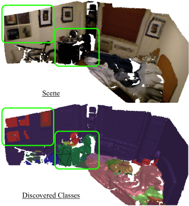
Figure 1: Proposed method incrementally discovers new classes (e.g., pictures) in the reconstructed 3D map.

Building a semantically annotated 3D map (i.e., semantic mapping) has become a vital research topic in computer vision and robotics communities since it provides 3D location information as well as object/scene category information. It is naturally very useful in a wide range of applications including robot navigation, mixed/virtual reality, and remote robot control. In most of these applications, it is important to achieve both high accuracy and efficiency. Considering robot navigation, robots need to recognize objects accurately and efficiently to navigate actively changing environments without any accident. In mixed reality systems, accuracy and efficiency are important to achieve more natural interactions without delay. When controlling surgical robots remotely, they are even more essential.

Consequently, many researches have been conducted to develop an accurate and efficient system for semantic mapping [15, 10, 20, 21, 29, 38, 41, 16, 18]. Most of the recent semantic mapping systems consist of two principal components, building a 3D map from RGBD images and processing semantic segmentation on either images or the built 3D maps [15, 10, 20, 21]. Since the introduction of RGBD sensors such as Microsoft Kinect [42], many approaches have been presented for building a 3D map from RGBD images [22, 12, 14, 17]. Regarding semantic segmentation, as semantic segmentation algorithms for images have been studied in many literatures, most semantic mapping systems have adapted these algorithms. Recently, since convolutional neural networks (CNNs) improve the performance of semantic segmentation further [19, 31, 4], CNNs have been incorporated to enhance the accuracy of semantic mapping [20, 21].

While these advancements improved the accuracy and efficiency of the overall system, the methods have limitations in the objects that the system can recognize. As previous semantic mapping systems recognize objects and scenes by training a pixel-level classifier (e.g., random forest or CNNs) using a training dataset, the systems are only able to recognize categories in the training dataset. This is a huge limitation for autonomous systems considering real-world consists of numerous objects/stuffs. Hence, we propose a novel system that can properly cluster both known objects and unseen things to enable discovering new categories. The proposed method first generates object-level segments in 3D. It then performs clustering of the object-level segments to associate objects of the same class and to discover new object classes.

The contributions of this paper are as follow: (1) We present, to the best of our knowledge, the first semantic mapping system that can properly discover clusters of both known objects and unseen objects in a 3D map (see Figure 1); (2) To effectively handle deep features and geometric cues in clustering, we propose to estimate the reliability of the deep features from CNNs using the entropy of the probability distribution from CNNs. We then use the estimated confidence for weighting the two types of features; (3) We propose to utilize segments instead of elements (i.e., surfel and voxel) in assigning/updating features and in clustering to efficiently reduce computational cost and space complexity. It enables the overall framework to run in semi-real-time; (4) We improve object proposals in a 3D map by utilizing both geometric and color information. It is especially important for the regions with poor geometric characteristics (e.g., pictures on a wall) ; (5) We demonstrate the effectiveness and efficiency of the proposed system by training CNNs on a subset of classes in a dataset and by discovering the other subset of classes by using the proposed method.

2 Related Work

Semantic Scene Reconstruction Koppula et al. presented one of the earliest works on semantic scene reconstruction using RGBD images [15]. Given multiple RGBD images, they first stitched the images to a single 3D point cloud. They then over-segmented the point cloud and labeled each segment using a graphical model.

As many 2D semantic segmentation approaches achieved impressive results [19, 31, 4], Hermans et al. proposed to use 2D semantic segmentation for 3D semantic reconstruction instead of segmenting 3D point clouds [10]. They first processed 2D semantic segmentation using randomized decision forests (RDF) and refined the result using a dense Conditional Random Fields (CRF). They then transferred class labels to 3D maps. Since, recently, convolutional neural networks (CNNs) further improved 2D semantic segmentation, McCormac et al. presented a system that utilizes CNNs for 2D semantic segmentation instead of RDF [20]. While we focus on semantic scene reconstruction methods using RGBD images, there are methods using stereo image pairs [29, 38, 41] and using a monocular camera [16, 18].

While all the previous works [15, 10, 20, 29, 38, 41, 16, 18] can recognize only learned object classes, we propose, to the best of our knowledge, the first semantic scene reconstruction system that can segment unseen object classes as well as trained classes.

Image Segmentation Image segmentation has been studied in many literatures [26, 32, 3, 7, 5, 8, 11, 9, 1, 2]. Relatively recently, Pont-Tuset et al. proposed an approach for bottom-up hierarchical image segmentation [24]. They developed a fast normalized cuts algorithm and also proposed a hierarchical segmenter that uses multiscale information. They then employed a grouping strategy that combines multiscale regions into highly-accurate object proposals. As convolutional neural networks (CNNs) have become a popular approach in semantic segmentation, Xia et al. proposed a CNN-based method for unsupervised image segmentation [39]. They segmented images by learning autoencoders with the consideration of the normalized cut and smoothed the segmentation outputs using a conditional random field. They then processed hierarchical segmentation that first converts over-segmented partitions into weighted boundary maps and then merges the most similar regions iteratively.

Considering RGBD data, Yang et al. proposed a two-stage segmentation method that consists of over-segmentation using 3-D geometry enhanced superpixels and graph-based merging [40]. They first applied a K-means-like clustering method to the RGBD data for over-segmentation using an 8-D distance metric constructed from both color and 3-D geometrical information. They then employed a graph-based model to relabel the superpixels into segments considering RGBD proximity, texture similarity, boundary continuity, and the number of labels.

Comparing to the previous works [26, 32, 3, 7, 5, 8, 11, 9, 1, 2, 24, 39, 40], this work differs from them in two aspects. First, we propose a segmentation algorithm for 3D reconstructed scenes rather than images. Second, we aim to group pixels with the same semantic meaning to a cluster even if they are distant or separated by another segment.

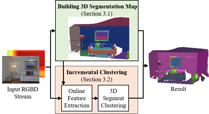
Figure 2: Overview of the proposed framework.

3 Class Discovery for Semantic Segmentation

In order to discover new classes of semantic segments, we need a method for aggregating and clustering unknown segments (i.e., segments of the image which cannot be classified into a known class). A central component of our proposed approach is the segmentation of a dense 3D reconstruction of the scene, which we call the 3D segmentation map, which is used to aggregate information about each 2D image segment and that information is used to perform the 3D segment clustering to discover new ‘semantic’ (a nameless category) classes.

To incrementally discover object classes using RGBD sensing, we first propose to build a 3D segmentation map for object-level segmentation in 3D. Second, we perform clustering of the object-level segments to associate objects of the same class and to discover new object classes. Figure 2 shows the overview of the proposed framework. Given an input RGBD stream, we build a 3D segmentation map (Section 3.1) and process incremental clustering (Section 3.2). The incremental clustering consists of extracting features for each frame (Section 3.2.1) and clustering using the features (Section 3.2.2). The output of the proposed method is the visualization of clustering membership on a reconstructed 3D map.

3.1 Building the 3D Segmentation Map

As mentioned above, the 3D segmentation map is the key data structure which is used to aggregate information about 2D image segmentation to discover new semantic classes. Building the 3D segmentation map is an incremental process, which consists of the following four processes applied to each frame: (1) SLAM for dense 3D map reconstruction; (2) SLIC for superpixel segmentation; (3) Agglomerative clustering; and (4) Updating the 3D segmentation map. We describe the details of each processing step below.

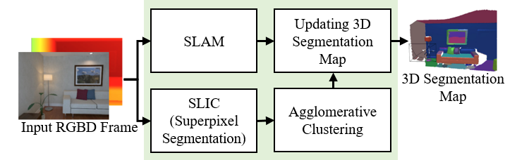
Figure 3: Building 3D Segmentation Map. The output of this processing is object-level segments in 3D. We build the 3D map by propagating 2D segmentation to the existing 3D segmentation map. (Section 3.1).

Dense SLAM. In order to estimate camera poses and incrementally build a 3D map, we employ the dense SLAM method, InfiniTAM v3 [25]. The method builds 3D maps using an efficient and scalable representation method which was proposed by Keller et al. [14]. The representation is a point-based description with normal information and is referred to as surfel. We denote surfels using $s_{k}$.

The surfel is a fundamental element in our reconstructed 3D map (like pixels on an image). Given a new depth frame, we generate surfels and fuse them into the existing reconstructed 3D map. Hence, building the 3D segmentation map includes building a reconstructed 3D map using SLAM and grouping surfels in the reconstructed 3D map.

RGBD SLIC. For every RGBD frame, we first implement a modified SLIC superpixel segmentation algorithm to generate roughly 250 superpixels (small image regions) for each frame. To use both color information and geometric cues, we define a new distance metric $D_{s}$ that uses the color image $\mathcal{I}^{lab}_{t}(\bm{u})\in\mathbb{R}^{3}$ in the CIELAB color space, the normal map $\mathcal{N}_{t}(\bm{u})\in\mathbb{R}^{3}$, and the image coordinates $\bm{u}=(x,y)\in\mathbb{Z}^{2}$. The distance $D_{s}$ between pixels $\bm{u}$ and $\bm{v}$ is computed as follows:

$$\begin{split}&D_{s}=d_{lab}+\alpha d_{n}+\beta d_{xy},\\ &d_{lab}=||\mathcal{I}^{lab}_{t}(\bm{u})-\mathcal{I}^{lab}_{t}(\bm{v})||_{2},\\ &d_{n}=||\mathcal{N}_{t}(\bm{u})-\mathcal{N}_{t}(\bm{v})||_{2},\\ &d_{xy}=||\bm{u}-\bm{v}||_{2},\end{split}$$ (1)

where $\alpha$ and $\beta$ are constants for weighting $d_{n}$ and $d_{xy}$. Given the set of superpixels from the SLIC segmentation, we compute the averaged color $\bm{c}^{lab}\in\mathbb{R}^{3}$, vertex $\bm{v}\in\mathbb{R}^{3}$, and normal $\bm{n}\in\mathbb{R}^{3}$ of each superpixel $r$, which will be used to further merge superpixels into bigger 2D regions.

Agglomerative Clustering. Since the SLIC superpixel segmentation tends to generate a grid of segments with similar sizes, we perform agglomerative clustering and merging to produce object-level segments. The clustering and merging are based on the similarity in $\bm{c}^{lab}$, $\bm{v}$, and $\bm{n}$ between superpixels. Specifically, we compute the similarity $\Lambda$ in color space, the geometric distance $\Psi$ in 3D space, and convexity $\Phi$ in shape. We then merge the superpixels if all the measured similarity/distances meet the following conditions.

Consider two neighboring superpixels $(r_{a},r_{b})$. The $\Lambda$, $\Psi$, and $\Phi$ are computed as follow:

$$\begin{split}&\Lambda(r_{a},r_{b})=||\bm{c}_{a}-\bm{c}_{b}||_{2},\\ &\Psi(r_{a},r_{b})=||(\bm{v}_{b}-\bm{v}_{a})\cdot\bm{n}_{a}||_{2},\\ &\Phi(r_{a},r_{b})=\left\{\begin{array}[]{ll}1&\text{if }(\bm{v}_{b}-\bm{v}_{a})\cdot\bm{n}_{a}>0,\\ \bm{n}_{a}\cdot\bm{n}_{b}&\mbox{otherwise.}\end{array}\right.\end{split}$$ (2)

Given $\Lambda$, $\Psi$, and $\Phi$, the pair of superpixels $(r_{a},r_{b})$ are merged only when they satisfy the predetermined criteria:

$$\Lambda<\sigma_{\Lambda}\text{ and }\Psi<\sigma_{\Psi}\text{ and }\Phi>\sigma_{\Phi},$$ (3)

where $\sigma_{\Lambda}$, $\sigma_{\Psi}$, and $\sigma_{\Phi}$ denote the corresponding thresholds for $\Lambda$, $\Psi$, and $\Phi$, respectively. Regarding convexity criteria, it is based on the observation that objects on captured images usually have convex shapes [36]. Consequently, we penalize merging regions with concave shapes. $\sigma_{\Psi}$ is computed using the noise model in [23], which presented the relationship between noise and distance from a sensor.

3D Segmentation Map Update. Given the 2D segmentation result of current frame, we update the 3D segmentation map. We employ the efficient and scalable segment propagation method in [36] to assign/update a segment label $l_{i}$ to each surfel $s_{k}$.

3.2 Incremental Clustering

In the previous section, we generate object-level segments by clustering and merging superpixels. The object-level segments are then used to update the 3D segmentation map. Given the object-level segments in the 3D segmentation map, incremental clustering aims to discover new object classes by clustering the object-level segments. To cluster the segments, we first extract features using an input RGBD frame and the 3D segmentation map. We then cluster by computing weighted similarity between the segments. We describe the details of online feature extraction in Section 3.2.1 and those of 3D segment clustering in Section 3.2.2 (also, see Figure 4).

3.2.1 Online Feature Extraction

In order to accurately associate objects of the same class or to discover new object classes, we need a method for estimating similarity between object segments in the 3D segmentation map. While measuring similarity can be as simple as computing distance in color space, more meaningful measurement is required to accurately determine object classes. Moreover, as objects often appear on multiple frames in a consecutive video, we can improve the similarity measurement by utilizing previous frames. Lastly, as record-keeping all the information from previous frames is expensive, we need an efficient method to store the past information.

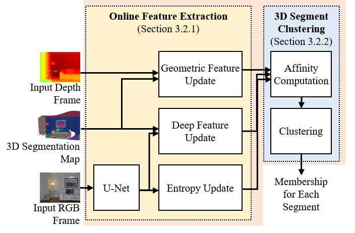
Figure 4: Incremental 3D Segment Clustering. This clustering is to associates objects of the same class or to discover new classes using object-level segments in the 3D segmentation map. (Section 3.2).

To estimate more meaningful similarity, we utilize both features from color images and geometric features as they are often complementary. Especially, as convolutional neural networks have achieved impressive results in per-pixel classification tasks [19, 31, 4], we extract features from color images using CNNs. The extracted deep features and geometric features for each frame are then used to update the features for each segment in the 3D segmentation map. By aggregating the features from all the previous frames, we improve the robustness of the features in the 3D segmentation map. Moreover, storing/updating the features for each segment is a very effective strategy for both saving memory usage and reducing computations for 3D segment clustering. Considering the number of segments is much smaller than that of surfels in the 3D map, the reduction in memory usages is very significant. Specifically, the memory usage is reduced from $O(N_{s}\textperiodcentered(S+G+1))$ to $O(N_{l}\textperiodcentered(S+G+1))$ where $N_{s}$ and $N_{l}$ denote the number of surfels and that of object-level segments in the 3D segmentation map, respectively; $S$ and $G$ represent the dimension of the deep features and that of the geometric features, respectively.

While CNNs have shown impressive results, the reliability of deep features can vary depending on the region of the input image. We hypothesize that the regions that CNNs can predict a class with high confidence, can be clustered accurately using deep features. Hence, we estimate the reliability of deep features using predicted probability distribution from CNNs. Specifically, we compute the confidence by calculating the entropy of the predicted probability distribution. We then, based on the estimated reliability, compute weighted affinity using the similarity of geometric feature and that of deep features between object-level segments in the 3D segmentation map.

For deep features and entropy, we employ the U-Net architecture [27] since our target applications (e.g. robot navigation) often demand short processing time. The network takes only $36ms$ to process an input image of $320\times 240$ resolution. Also, by using the same network for both processing, we can save computations.

Geometric Feature Extraction/Update. To extract translation/rotation-invariant and noise-robust geometric features, we first estimate a Local Reference Frame (LRF) for each segment. We then extract geometric features for each segment using a fast and unique geometric feature descriptor, Global Orthographic Object Descriptor (GOOD) [13].

Given a depth map, to estimate LRF for each segment, we need the 3D segmentation map on the current image plane. Hence, we first render the segmentation map to the current image plane and obtain the rendered segmentation map $\mathcal{R}$ with segment labels $l_{i}$. We then compute the LRF by processing the Principal Component Analysis (PCA) for each segment. In more details about processing the PCA, we first compute the normalized covariance matrix and then perform eigenvalue decomposition. The normalized covariance matrix $\bm{C}_{l_{i}}$ of each segment $l_{i}$ is computed using the vertex map $\mathcal{V}_{t}$ and the rendered segmentation map $\mathcal{R}$ as follows:

$$\begin{split}\bm{C}_{l_{i}}&=\frac{1}{|\mathcal{U}_{l_{i}}|}\sum_{\bm{v}\in\mathcal{U}_{l_{i}}}(\bm{v}-\bm{o}_{l_{i}})(\bm{v}-\bm{o}_{l_{i}})^{T},\\ \bm{o}_{l_{i}}&=\frac{1}{|\mathcal{U}_{l_{i}}|}\sum_{\bm{v}\in\mathcal{U}_{l_{i}}}\bm{v},\\ \mathcal{U}_{l_{i}}&=\{\mathcal{V}_{t}(\bm{u})|\mathcal{R}(\bm{u})=l_{i}\},\end{split}$$ (4)

where $\bm{o}_{l_{i}}$ represents the geometric center of the segment $l_{i}$; $\mathcal{U}_{l_{i}}$ denotes the set of vertices that belong to the segment $l_{i}$ on the current frame; $|\cdot|$ represents the number of elements in the set. We then perform eigenvalue decomposition on $\bm{C}_{l_{i}}$ as follows:

$$\bm{C}_{l_{i}}\bm{X}_{l_{i}}=\bm{E}_{l_{i}}\bm{X}_{l_{i}},$$ (5)

where $\bm{X}_{l_{i}}$ is a matrix with three eigenvectors; $\bm{E}_{l_{i}}=diag(\lambda_{1},\lambda_{2},\lambda_{3})$ is a diagonal matrix with the corresponding eigenvalues. $\bm{X}_{l_{i}}$ is directly utilized as the LRF.

Lastly, we employ a fast and unique geometric feature descriptor, GOOD [13]. For each $l_{i}$, we transform the set of vertices $\mathcal{U}_{l_{i}}$ using the LRF. We then fed the transformed vertices into the descriptor to obtain the frame-wise geometric feature $\mathcal{F}^{\text{GEO}}_{t}(l_{i})\in\mathbb{R}^{75}$.

After computing $\mathcal{F}^{\text{GEO}}_{t}(l_{i})$ using the current depth map, the geometric features $\bm{f}^{\text{GEO}}_{l_{i}}$ in the 3D segmentation map are updated as follows:

$$\begin{split}&\bm{f}^{\text{GEO}}_{l_{i}}\leftarrow\frac{1}{Z^{\text{GEO}}_{l_{i}}}\cdot\frac{\Omega\bm{f}^{\text{GEO}}_{l_{i}}+\mathcal{F}^{\text{GEO}}_{t}(l_{i})}{\Omega+1},\\ &\Omega\leftarrow\Omega+1.\end{split}$$ (6)

This updates are applied to all segments $l_{i}$ on the rendered segmentation map $\mathcal{R}$. $Z^{\text{GEO}}_{l_{i}}$ denotes the constant for normalizing the feature vector $\bm{f}^{\text{GEO}}_{l_{i}}$.

Deep Feature Extraction/Update. We utilize the output of the layer just before the last classification layer for deep feature map. The per-frame deep feature map is denoted as $\mathcal{F}^{\text{CNN}}_{t}(\bm{u})\in\mathbb{R}^{S}$. The size of $\mathcal{F}^{\text{CNN}}_{t}$ is $W\times H\times S$ where $W$ and $H$ represent the width and height of an input image, respectively; and $S$ denotes the number of channels (i.e. the dimension of the features) which is $64$.

We update the deep features $\bm{f}^{\text{CNN}}_{l_{i}}$ for each segment $l_{i}$ in the 3D segmentation map by employing incremental averaging approach and by using the per-frame deep features. Since deep features and entropy are extracted for each pixel while geometric features are obtained for each segment $l_{i}$, the procedures for updating are slightly different. The deep features $\bm{f}^{\text{CNN}}_{l_{i}}$ are updated as follows:

$$\begin{split}&\bm{f}^{\text{CNN}}_{l_{i}=\mathcal{R}(\bm{u})}\leftarrow\frac{1}{Z^{\text{CNN}}_{l_{i}}}\cdot\frac{\Gamma\bm{f}^{\text{CNN}}_{l_{i}=\mathcal{R}(\bm{u})}+\mathcal{F}^{\text{CNN}}_{t}(\bm{u})}{\Gamma+1},\\ &\Gamma\leftarrow\Gamma+1,\end{split}$$ (7)

where $Z^{\text{CNN}}_{l_{i}}$ is the normalizing constant for $\bm{f}^{\text{CNN}}_{l_{i}}$; $\bm{u}$ is all the coordinates on $\mathcal{F}^{\text{CNN}}_{t}$.

Entropy Computation/Update. The entropy is computed by first estimating the probability distribution for each class and by measuring the Shannon entropy [30] using the probability distribution. As the network is trained for semantic segmentation, the probability distribution is obtained by the output of the softmax layer of the network. The entropy $\mathcal{E}(\bm{u})\in\mathbb{R}$ is computed at each pixel $\bm{u}$ as follows:

$$\mathcal{E}(\bm{u})=-\sum_{c}P_{c}(\bm{u})\log P_{c}(\bm{u}),$$ (8)

where $P_{c}(\bm{u})\in\mathbb{R}$ is the probability for the class $c$ at the pixel $\bm{u}$. Then, $\mathcal{E}(\bm{u})$ is used for updating the entropy $e_{l_{i}}$ for each segment $l_{i}$ in the 3D segmentation map as follows:

$$\begin{split}&e_{l_{i}=\mathcal{R}(\bm{u})}\leftarrow\frac{\Gamma e_{l_{i}=\mathcal{R}(\bm{u})}+\mathcal{E}(\bm{u})}{\Gamma+1},\\ &\Gamma\leftarrow\Gamma+1,\end{split}$$ (9)

where $\bm{u}$ is all the coordinates on $\mathcal{E}$.

Table 1: Quantitative comparison on the NYUDv2 dataset [33]. Supervised methods versus unsupervised methods (ours).

Method	classes in training dataset									novel classes				mean
	bed	book	chair	floor	furn.	obj.	sofa	table	wall	ceil.	pict.	tv	wind.	IoU
U-Net [27]	50.32	22.42	36.55	55.62	36.85	27.27	48.44	33.78	55.14	-	-	-	-	-
Nakajima et al. [21]	62.82	27.27	42.56	68.43	44.62	24.63	45.04	42.30	26.82	-	-	-	-	-
Ours + 3D Map  [36]	62.80	23.96	33.10	63.41	50.58	27.28	58.68	40.23	54.53	31.42	19.37	43.98	31.30	41.59
Ours	64.22	22.28	41.79	67.38	56.15	28.61	49.31	40.95	63.18	29.30	28.69	52.20	53.92	46.05

3.2.2 3D Segment Clustering

Given semantic and geometric features in the 3D segmentation map from the feature updating stage, we apply a graph-based unsupervised clustering algorithm to cluster regions in the 3D segmentation map. We specifically employ the Markov clustering algorithm (MCL) [37] because of the flexible number of clusters and computational cost. Since we aim to be able to handle unknown objects in a scene, we need the number of clusters (class categories) to be flexible, like the MCL. Furthermore, since the computational cost $O(M^{3})$ of the MCL comes from the multiplication of two matrices with the size $M\times M$, where $M$ denotes the number of nodes in the graph, the cost can be turned into $O(M)$ by parallelizing the processing in a GPU. Accordingly, it reduces processing time and makes more appropriate for an online system.

We define the similarity $s(i,j)$ between nodes (i.e. regions $l_{i}$ and $l_{j}$ in the 3D segmentation map). The weight values $w_{i}$ and $w_{j}$ are first computed using the entropy $e$ and the number $N$ of classes in the training dataset for the U-Net as follows:

$$w_{i}=\frac{e_{l_{i}}}{\log N},\ w_{j}=\frac{e_{l_{j}}}{\log N}.$$ (10)

The denominator $\log N$ is selected to make $w$ to be in [0,1] considering the maximum value of $e_{l_{i}}$ is $\log N$. The similarity $s(i,j)$ is then defined using $w_{i}$ and $w_{j}$ as follows:

$$\begin{split}s(i,j)&=e^{-\eta d(i,j)},\\ d(i,j)&=||(1-w_{i})\bm{f}^{\text{CNN}}_{l_{i}}-(1-w_{j})\bm{f}^{\text{CNN}}_{l_{j}}||_{2}\\ &+||w_{i}\bm{f}^{\text{GEO}}_{l_{i}}-w_{j}\bm{f}^{\text{GEO}}_{l_{j}}||_{2},\end{split}$$ (11)

where $\eta$ is a predefined constant. Based on the assumption that the entropies of regions belonging to unknown object categories are high, the similarity measurement between these regions is more relying on geometric features than deep features. We calculate the similarity $s(i,j)$ for each pair of region $(i,j)$ and feed the similarities to the MCL to update clusters.

4 Experiments and Results

Table 2: Ablation study on effects of deep features and geometric features for clustering.

o 1.22X[l,m]—ccccccccc—cccc—c   Method	classes in training dataset									novel classes
	bed	book	chair	floor	furn.	obj.	sofa	table	wall	ceil.	pict.	tv	wind.	mean IoU
Ours GEO-only	51.95	21.47	35.99	64.75	50.28	28.36	48.98	39.14	55.80	29.76	25.38	44.88	52.43	42.24
Ours CNN-only	60.07	28.23	37.55	63.53	49.48	30.16	51.21	43.59	59.94	20.82	22.60	39.41	42.30	42.22
Ours	64.22	22.28	41.79	67.38	56.15	28.61	49.31	40.95	63.18	29.30	28.69	52.20	53.92	46.05

To demonstrate the ability of discovering new object classes using RGBD sensing, we experiment on a publicly available RGBD dataset [33]. We first train a semantic segmentation network using only a subset of object classes. We then apply the proposed method to discover both the trained clases and unseen classes. We demonstrate the effectiveness of the proposed method by measuring accuracy, processing time, and memory footprint on a test dataset. All accuracy evaluations are performed at 320 $\times$ 240 resolution. Processing time is measured using a machine with an Intel Core i7-5557U 3.1GHz CPU, GeForce GTX 1080 GPU, and 16GB RAM. We use the following thresholds and constant for all the experiments: $\sigma_{\Lambda}=7.0,\sigma_{\Phi}=0.8,\eta=6.0,\alpha=110.0,\beta=0.5$.

Dataset. We experiment our system using the publicly available NYUDv2 dataset [33] which consists of 206 test video sequences. Since many of the videos have significant drops in frame-rate, they are inappropriate for tracking and reconstruction. Accordingly, previous works [10, 20, 21] have used only 140 test sequences that have at least 2 frames per second. This results in 360 labeled test images from the 654 images in the original test set.

U-Net Training. To evaluate the proposed system’s ability of class discovering, we train the U-Net using a subset of classes and evaluate the system using entire classes. This enables the quantitative analysis of both trained classes and unseen classes. We train the U-Net using the SUN RGBD training dataset [35] which consists of 5,285 RGBD images. We first initialize the weights of the U-Net using the VGG model [34] trained on the ILSVRC dataset [28]. We then finetune the model using pre-selected 9 classes among the 13 classes defined in [6]. The selected classes and the entire classes are shown in Table 1. The same trained model is used for both the proposed method and comparing methods [27, 21] in Section 4.1.

4.1 Results

We experimentally demonstrate the performance of the proposed method quantitatively and qualitatively. For quantitative comparison, we measure the Intersection over Union (IoU) using the test set of the NYUDv2 dataset [33] and present on Table 1 and Table 4. In Table 1, we compare the proposed method with two fully supervised methods and our methods with a different incremental 3D segmentation method [36]. For the supervised methods, we selected one state-of-the-art semantic mapping method [21] and one semantic segmentation method [27] for 2D images. Obviously, these methods can only predict for the 9 classes in the training dataset. As we propose a novel method for building a geometric 3D map using an RGBD SLIC-based segmentation method, we compare the proposed method with the method with the previous incremental 3D segmentation method of [36]. Since [36] uses only depth maps excluding color information, our method outperforms largely for the classes with poor geometric characteristics (e.g., picture and window). Hence, it verifies the effectiveness of the proposed SLIC-based incremental segmentation approach. Overall, the proposed method achieves competitive accuracy comparing to the state-of-the-art supervised method [21] and is able to successfully discover novel categories for unseen objects. Also, the proposed method outperforms the method with [36] by 4.46 in mean IoU.

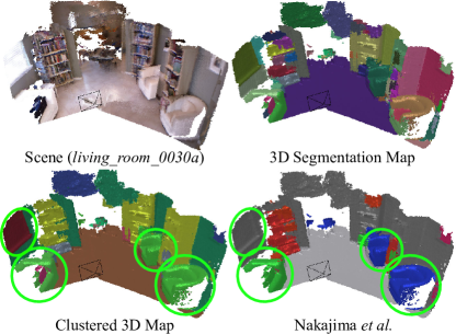
Figure 5: Qualitative results of dense 3D incremental semantic mapping. The proposed method discovers various classes including both unseen classes and the classes in the training dataset of the U-Net. For the geometric 3D map and the clustered 3D map, a distinctive color is used for each segment and each cluster, respectively. For the results of Nakajima et al. [21], which is a fully supervised method, a specific color is used for each category as shown in Table 1.

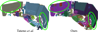
Figure 6: Qualitative results of the 3D segmentation map. The proposed method successfully segments pictures and the headboard of a bed which have poor geometric characteristics while [36] has limitation.

In Table 4, we compare the results of the proposed method to those using only geometric features (Ours GEO-only) and those using only deep features (Ours CNN-only) to demonstrate the effectiveness of properly utilizing both features for measuring the similarity in (11). By comparing “Ours GEO-only” and “Ours CNN-only”, we can observe that “Ours CNN-only” achieves higher or similar accuracy comparing to “Ours GEO-only” in the trained classes and “Ours GEO-only” outperforms “Ours CNN-only” for all the unseen classes. It consequently demonstrates the importance of effectively utilizing both CNN features and geometric features to achieve high accuracy in both trained classes and unseen classes. By applying the proposed confidence estimation, the proposed method achieves higher accuracy comparing to “Ours GEO-only” and “Ours CNN-only” in most of the classes. It verifies the effectiveness of weighting deep features and geometric features based on the estimated confidence using the entropy. The proposed method achieves 3.81 and 3.83 higher mean IoU comparing to “Ours GEO-only” and “Ours CNN-only”, respectively.

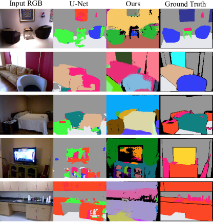
Figure 7: Qualitative comparison on the NYUDv2 dataset [33]. To visualize the results of the proposed method, we use a different color for each cluster. The results of the U-Net and the ground truth labels are visualized using a specific color for each category as shown in Table 1.

Figures 1, 5, 6, and 7 show qualitative results of the proposed method and comparing methods. The figures demonstrate that the proposed method properly clusters objects of both trained classes (for U-Net) and unseen classes. Distinctive trained objects include the chair in Figure 5 and the desk on Figure 1. Characteristic unseen objects include the window in Figure 5 and the pictures in Figure 1. Moreover, Figure 6 shows the comparison between the proposed method and [36] in building 3D segmentation map for object proposal generation. It shows that the proposed method can segment the regions even with poor geometric characteristics (e.g., pictures on the wall) by utilizing both depth and color cues while [36] has limitations.

The bottom two rows of Figure 7 show the failure cases of the proposed method. On the fourth row, while the proposed method successfully segments and makes a cluster for the TV (unseen object), the furniture under the TV is segmented and grouped into multiple clusters because of the glasses on the furniture. On the fifth row, the small objects on the countertop are not segmented accurately. These kinds of objects are challenging since they are distant from the depth sensor and are small size, which often leads to less accurate depth sensing.

4.2 Run-time Performance and Memory Footprint

We demonstrate the efficiency of the proposed method by measuring processing time and memory footprint. The average processing time for each stage is shown in Table 3. The total processing time is 93.2 ms (10.7Hz) on average. By the strategy of clustering segments instead of elements, we were able to effectively reduce the processing time of 3D segment clustering to 13.4 ms on average. The average number of segments in a 3D map was $253.7$. The two most expensive processing are forward-processing of the U-Net and the feature updating.

Table 3: Average processing time for each stage. Note that the processing with * and that with ** can be processed simultaneously.

Component	Processing time
Building 3D segmentation map *	18.2 ms
Deep feature extraction **	35.9 ms
Geometric feature extraction	8.2 ms
Entropy computation	2.3 ms
Feature/Entropy update	33.4 ms
3D segment clustering	13.4 ms
Total	93.2 ms

We also present the processing time on Figure 8 and the memory footprint on Figure 9 for each frame in a sequence. Figure 8 shows that the processing time is quite stable even though the reconstructed 3D map increases. Figure 9 shows the memory footprint for storing deep features and geometric features. We compare the proposed method with the baseline method which assigns/updates features to each element similar to [10, 20]. The analysis verifies that storing features for each segment significantly suppressed memory usage comparing to storing feature for each element. As shown in Section 3.2.1, the space complexity of the proposed method is $O(N_{l}\cdot(S+G+1))$ while that of the baseline method is $O(N_{s}\cdot(S+G+1))$. After reconstructing all the frames in the sequence bedroom_0018b, $N_{l}$ and $N_{s}$ are 196 and 900,478, respectively.

Figure 8: Processing time for each frame of the sequence bedroom_0018b in the NYUDv2 dataset [33].

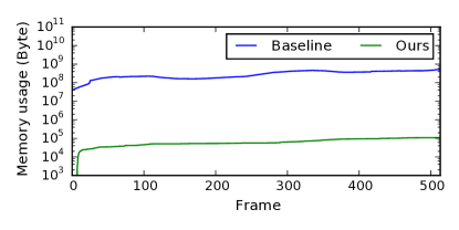
Figure 9: Comparison of memory usage for storing semantic and geometric features using the sequence bedroom_0018b in the NYUDv2 dataset [33]. While the proposed method assigns/updates features to each segment of the 3D map, the baseline method assigns/updates features to each element similar to [10, 20] which assign class probabilities to each element.

5 Conclusion

Towards open world semantic segmentation, we present a novel method that incrementally discovers new classes using RGBD sensing. We propose to discover new object classes by building a segmented dense 3D map and by identifying coherent regions in the 3D map. We demonstrate that the proposed method is able to successfully discover new object classes by experimenting on a public dataset. The experimental results also show that the proposed method achieves competitive accuracy for known classes comparing to the supervised methods. We further show that the proposed method is very efficient in computation and memory usage.

References

- [1] P. Arbelaez, M. Maire, C. Fowlkes, and J. Malik. From contours to regions: An empirical evaluation. In 2009 IEEE Conference on Computer Vision and Pattern Recognition, pages 2294–2301, June 2009.
- [2] P. Arbelaez, M. Maire, C. Fowlkes, and J. Malik. Contour detection and hierarchical image segmentation. IEEE Transactions on Pattern Analysis and Machine Intelligence, 33(5):898–916, May 2011.
- [3] Y. Boykov, O. Veksler, and R. Zabih. Fast approximate energy minimization via graph cuts. IEEE Transactions on Pattern Analysis and Machine Intelligence, 23(11):1222–1239, Nov 2001.
- [4] L. Chen, G. Papandreou, I. Kokkinos, K. Murphy, and A. L. Yuille. Deeplab: Semantic image segmentation with deep convolutional nets, atrous convolution, and fully connected crfs. IEEE Transactions on Pattern Analysis and Machine Intelligence, 40(4):834–848, April 2018.
- [5] D. Comaniciu and P. Meer. Mean shift: a robust approach toward feature space analysis. IEEE Transactions on Pattern Analysis and Machine Intelligence, 24(5):603–619, May 2002.
- [6] C. Couprie, C. Farabet, L. Najman, and Y. LeCun. Indoor semantic segmentation using depth information. In International Conference on Learning Representations, 2013.
- [7] Y. Deng and B. S. Manjunath. Unsupervised segmentation of color-texture regions in images and video. IEEE Transactions on Pattern Analysis and Machine Intelligence, 23(8):800–810, Aug 2001.
- [8] P. F. Felzenszwalb and D. P. Huttenlocher. Efficient graph-based image segmentation. International Journal of Computer Vision, 59(2):167–181, Sep 2004.
- [9] B. Fulkerson and S. Soatto. Really quick shift: Image segmentation on a gpu. In K. N. Kutulakos, editor, Trends and Topics in Computer Vision, pages 350–358, Berlin, Heidelberg, 2012. Springer Berlin Heidelberg.
- [10] A. Hermans, G. Floros, and B. Leibe. Dense 3d semantic mapping of indoor scenes from rgb-d images. In 2014 IEEE International Conference on Robotics and Automation (ICRA), pages 2631–2638, May 2014.
- [11] Y.-L. Huang and D.-R. Chen. Watershed segmentation for breast tumor in 2-d sonography. Ultrasound in Medicine and Biology, 30(5):625 – 632, 2004.
- [12] S. Izadi, D. Kim, O. Hilliges, D. Molyneaux, R. Newcombe, P. Kohli, J. Shotton, S. Hodges, D. Freeman, A. Davison, and A. Fitzgibbon. Kinectfusion: Real-time 3d reconstruction and interaction using a moving depth camera. In Proceedings of the 24th Annual ACM Symposium on User Interface Software and Technology, UIST ’11, pages 559–568, New York, NY, USA, 2011. ACM.
- [13] S. H. Kasaei, A. M. Tomé, L. S. Lopes, and M. Oliveira. Good: A global orthographic object descriptor for 3d object recognition and manipulation. Pattern Recognition Letters, 83:312–320, 2016.
- [14] M. Keller, D. Lefloch, M. Lambers, S. Izadi, T. Weyrich, and A. Kolb. Real-time 3d reconstruction in dynamic scenes using point-based fusion. In 2013 International Conference on 3D Vision - 3DV 2013, pages 1–8, June 2013.
- [15] H. S. Koppula, A. Anand, T. Joachims, and A. Saxena. Semantic labeling of 3d point clouds for indoor scenes. In J. Shawe-Taylor, R. S. Zemel, P. L. Bartlett, F. Pereira, and K. Q. Weinberger, editors, Advances in Neural Information Processing Systems 24, pages 244–252. Curran Associates, Inc., 2011.
- [16] A. Kundu, Y. Li, F. Dellaert, F. Li, and J. M. Rehg. Joint semantic segmentation and 3d reconstruction from monocular video. In D. Fleet, T. Pajdla, B. Schiele, and T. Tuytelaars, editors, Computer Vision – ECCV 2014, pages 703–718, Cham, 2014. Springer International Publishing.
- [17] K.-R. Lee and T. Nguyen. Realistic surface geometry reconstruction using a hand-held rgb-d camera. Machine Vision and Applications, 27(3):377–385, Apr 2016.
- [18] X. Li, H. Ao, R. Belaroussi, and D. Gruyer. Fast semi-dense 3d semantic mapping with monocular visual slam. In 2017 IEEE 20th International Conference on Intelligent Transportation Systems (ITSC), pages 385–390, Oct 2017.
- [19] J. Long, E. Shelhamer, and T. Darrell. Fully convolutional networks for semantic segmentation. In 2015 IEEE Conference on Computer Vision and Pattern Recognition (CVPR), pages 3431–3440, June 2015.
- [20] J. McCormac, A. Handa, A. Davison, and S. Leutenegger. Semanticfusion: Dense 3d semantic mapping with convolutional neural networks. In 2017 IEEE International Conference on Robotics and Automation (ICRA), pages 4628–4635, May 2017.
- [21] Y. Nakajima, K. Tateno, F. Tombari, and H. Saito. Fast and accurate semantic mapping through geometric-based incremental segmentation. In 2018 IEEE/RSJ International Conference on Intelligent Robots and Systems (IROS), pages 385–392, Oct 2018.
- [22] R. A. Newcombe, S. Izadi, O. Hilliges, D. Molyneaux, D. Kim, A. J. Davison, P. Kohi, J. Shotton, S. Hodges, and A. Fitzgibbon. Kinectfusion: Real-time dense surface mapping and tracking. In 2011 10th IEEE International Symposium on Mixed and Augmented Reality, pages 127–136, Oct 2011.
- [23] C. V. Nguyen, S. Izadi, and D. Lovell. Modeling kinect sensor noise for improved 3d reconstruction and tracking. In 2012 second international conference on 3D imaging, modeling, processing, visualization & transmission, pages 524–530. IEEE, 2012.
- [24] J. Pont-Tuset, P. Arbeláez, J. T. Barron, F. Marques, and J. Malik. Multiscale combinatorial grouping for image segmentation and object proposal generation. IEEE Transactions on Pattern Analysis and Machine Intelligence, 39(1):128–140, Jan 2017.
- [25] V. A. Prisacariu, O. Kähler, S. Golodetz, M. Sapienza, T. Cavallari, P. H. S. Torr, and D. W. Murray. Infinitam v3: A framework for large-scale 3d reconstruction with loop closure. CoRR, abs/1708.00783, 2017.
- [26] S. Ray and R. H. Turi. Determination of number of clusters in k-means clustering and application in colour segmentation. In The 4th International Conference on Advances in Pattern Recognition and Digital Techniques, pages 137–143, 1999.
- [27] O. Ronneberger, P. Fischer, and T. Brox. U-net: Convolutional networks for biomedical image segmentation. In N. Navab, J. Hornegger, W. M. Wells, and A. F. Frangi, editors, Medical Image Computing and Computer-Assisted Intervention – MICCAI 2015, pages 234–241, Cham, 2015. Springer International Publishing.
- [28] O. Russakovsky, J. Deng, H. Su, J. Krause, S. Satheesh, S. Ma, Z. Huang, A. Karpathy, A. Khosla, M. Bernstein, A. C. Berg, and L. Fei-Fei. Imagenet large scale visual recognition challenge. International Journal of Computer Vision, 115(3):211–252, Dec 2015.
- [29] S. Sengupta, E. Greveson, A. Shahrokni, and P. H. S. Torr. Urban 3d semantic modelling using stereo vision. In 2013 IEEE International Conference on Robotics and Automation, pages 580–585, May 2013.
- [30] C. E. Shannon. A mathematical theory of communication. Bell System Technical Journal, 27(3):379–423, 1948.
- [31] E. Shelhamer, J. Long, and T. Darrell. Fully convolutional networks for semantic segmentation. IEEE Transactions on Pattern Analysis and Machine Intelligence, 39(4):640–651, April 2017.
- [32] J. Shi and J. Malik. Normalized cuts and image segmentation. IEEE Transactions on Pattern Analysis and Machine Intelligence, 22(8):888–905, Aug 2000.
- [33] N. Silberman, D. Hoiem, P. Kohli, and R. Fergus. Indoor segmentation and support inference from rgbd images. In A. Fitzgibbon, S. Lazebnik, P. Perona, Y. Sato, and C. Schmid, editors, Computer Vision – ECCV 2012, pages 746–760, Berlin, Heidelberg, 2012. Springer Berlin Heidelberg.
- [34] K. Simonyan and A. Zisserman. Very deep convolutional networks for large-scale image recognition. In International Conference on Learning Representations, 2015.
- [35] S. Song, S. P. Lichtenberg, and J. Xiao. Sun rgb-d: A rgb-d scene understanding benchmark suite. In 2015 IEEE Conference on Computer Vision and Pattern Recognition (CVPR), pages 567–576, June 2015.
- [36] K. Tateno, F. Tombari, and N. Navab. Real-time and scalable incremental segmentation on dense slam. In 2015 IEEE/RSJ International Conference on Intelligent Robots and Systems (IROS), pages 4465–4472, Sep. 2015.
- [37] S. van Dongen. Graph clustering by flow simulation. University of Utrecht, 2000.
- [38] V. Vineet, O. Miksik, M. Lidegaard, M. Nießner, S. Golodetz, V. A. Prisacariu, O. Kähler, D. W. Murray, S. Izadi, P. Pérez, and P. H. S. Torr. Incremental dense semantic stereo fusion for large-scale semantic scene reconstruction. In 2015 IEEE International Conference on Robotics and Automation (ICRA), pages 75–82, May 2015.
- [39] X. Xia and B. Kulis. W-net: A deep model for fully unsupervised image segmentation. CoRR, abs/1711.08506, 2017.
- [40] J. Yang, Z. Gan, K. Li, and C. Hou. Graph-based segmentation for rgb-d data using 3-d geometry enhanced superpixels. IEEE Transactions on Cybernetics, 45(5):927–940, May 2015.
- [41] S. Yang, Y. Huang, and S. Scherer. Semantic 3d occupancy mapping through efficient high order crfs. In 2017 IEEE/RSJ International Conference on Intelligent Robots and Systems (IROS), pages 590–597, Sep. 2017.
- [42] Z. Zhang. Microsoft kinect sensor and its effect. IEEE MultiMedia, 19(2):4–10, Feb 2012.