EUROPEAN ORGANIZATION FOR NUCLEAR RESEARCH (CERN)

​​​ CERN-EP-2019-121 LHCb-PAPER-2019-019 23 July 2019

Measurement of $C\!P$ violation in the ${{B}^{0}_{s}}\!\rightarrow\phi\phi$ decay and search for the ${{B}^{0}}\rightarrow\phi\phi$ decay

LHCb collaboration

A measurement of the time-dependent $C\!P$-violating asymmetry in ${{B}^{0}_{s}}\rightarrow\phi\phi$ decays is presented. Using a sample of proton-proton collision data corresponding to an integrated luminosity of $5.0\text{\,fb}^{-1}$ collected by the LHCb experiment at centre-of-mass energies $\sqrt{s}=7$  TeV in 2011, 8  TeV in 2012 and 13  TeV in 2015 and 2016, a signal yield of around 9000 ${{B}^{0}_{s}}\!\rightarrow\phi\phi$ decays is obtained. The $C\!P$-violating phase $\phi_{s}^{s\bar{s}s}$ is measured to be $-0.073\pm 0.115\text{\,(stat)}\pm 0.027\text{\,(syst)}\text{\,rad}$, under the assumption it is independent of the helicity of the $\phi\phi$ decay. In addition, the $C\!P$-violating phases of the transverse polarisations under the assumption of $C\!P$ conservation of the longitudinal phase are measured. The helicity-independent direct $C\!P$-violation parameter is also measured, and is found to be $|\lambda|=0.99\pm 0.05\text{\,(stat)}\pm 0.01\text{\,(syst)}$. In addition, $T$-odd triple-product asymmetries are measured. The results obtained are consistent with the hypothesis of $C\!P$ conservation in ${\overline{b}}\rightarrow{\overline{s}}{{s}{\overline{s}}}$ transitions. Finally, a limit on the branching fraction of the ${{B}^{0}}\rightarrow\phi\phi$ decay is determined to be $\mathcal{B}({{B}^{0}}\rightarrow\phi\phi)<2.7\times 10^{-8}$ at 90 % confidence level.

Published in JHEP 12 (2019) 155

© 2024 CERN for the benefit of the LHCb collaboration. CC-BY-4.0 licence.

 

1 Introduction

In the Standard Model (SM) the ${{B}^{0}_{s}}\rightarrow\phi\phi$ decay, where the $\phi(1020)$ is implied throughout this paper, is forbidden at tree level and proceeds predominantly via a gluonic ${\overline{b}}\rightarrow{\overline{s}}{{s}{\overline{s}}}$ loop (penguin) process. Hence, this channel provides an excellent probe of new heavy particles entering the penguin quantum loops [1, 2, 3]. In the SM, $C\!P$ violation is governed by a single phase in the Cabibbo–Kobayashi–Maskawa quark mixing matrix [4, *Cabibbo:1963yz]. Interference caused by the resulting weak phase difference between the ${B}^{0}_{s}$-${\kern 1.79993pt\overline{\kern-1.79993ptB}}{}^{0}_{s}$ oscillation and decay amplitudes leads to a $C\!P$ asymmetry in the decay-time distributions of ${{B}^{0}_{s}}$ and ${{\kern 1.79993pt\overline{\kern-1.79993ptB}}{}^{0}_{s}}$ mesons. For ${{B}^{0}_{s}}\rightarrow{{J\mskip-3.0mu/\mskip-2.0mu\psi\mskip 2.0mu}}{{K}^{+}}{{K}^{-}}$ and ${{B}^{0}_{s}}\rightarrow{{J\mskip-3.0mu/\mskip-2.0mu\psi\mskip 2.0mu}}{{\pi}^{+}}{{\pi}^{-}}$ decays, which proceed via ${\overline{b}}\rightarrow{\overline{s}}{{c}{\overline{c}}}$ transitions, the SM prediction of the weak phase is $-2\arg\left(-V_{ts}V_{tb}^{*}/V_{cs}V_{cb}^{*}\right)=-0.0369^{+0.0010}_{-0.0007}\;\rm rad$ according to the CKMfitter group [6], and $-2\arg\left(-V_{ts}V_{tb}^{*}/V_{cs}V_{cb}^{*}\right)=-0.0370\pm 0.0010\;\rm rad$ according to the UTfit collaboration [7]. The LHCb collaboration has measured the weak phase in several decay processes: ${{B}^{0}_{s}}\rightarrow{{J\mskip-3.0mu/\mskip-2.0mu\psi\mskip 2.0mu}}{{K}^{+}}{{K}^{-}}$, ${{B}^{0}_{s}}\rightarrow{{J\mskip-3.0mu/\mskip-2.0mu\psi\mskip 2.0mu}}{{\pi}^{+}}{{\pi}^{-}}$, ${{B}^{0}_{s}}\rightarrow{{J\mskip-3.0mu/\mskip-2.0mu\psi\mskip 2.0mu}}{{K}^{+}}{{K}^{-}}$ for the ${{K}^{+}}{{K}^{-}}$ invariant mass region above 1.05 $\text{\,Ge\kern-1.00006ptV\!/}c$, ${{B}^{0}_{s}}\rightarrow\psi(2S)\phi$ and ${{B}^{0}_{s}}\rightarrow D_{s}^{+}D_{s}^{-}$, corresponding to the combined result of $-0.041\pm 0.025\text{\,rad}$ [8]. These measurements are consistent with the SM prediction and place stringent constraints on $C\!P$ violation in ${B}^{0}_{s}$-${\kern 1.79993pt\overline{\kern-1.79993ptB}}{}^{0}_{s}$ oscillations [9]. The $C\!P$-violating phase, $\phi_{{s}}^{{{s}{\overline{s}}}{s}}$, in the ${{B}^{0}_{s}}\!\rightarrow\phi\phi$ decay is expected to be small in the SM. Calculations using quantum chromodynamics factorisation (QCDf) provide an upper limit of $0.02\text{\,rad}$ for its absolute value [1, 2, 3]. The previous most accurate measurement is ${\phi_{{s}}^{{{s}{\overline{s}}}{s}}}=-0.17\pm 0.15\text{\,(stat)}\pm 0.03\text{\,(syst)}\text{\,rad}$ [10].

$C\!P$ violation can also be probed by time-integrated triple-product asymmetries. These are formed from $T$-odd combinations of the momenta of the final-state particles. These asymmetries complement the decay-time-dependent measurement [11] and are expected to be close to zero in the SM [12]. Previous measurements of the triple-product asymmetries in ${B}^{0}_{s}$ decays from the LHCb and CDF collaborations [10, 13] have shown no significant deviations from zero.

The ${{B}^{0}_{s}}\!\rightarrow\phi\phi$ decay is a $P\rightarrow VV$ decay, where $P$ denotes a pseudoscalar and $V$ a vector meson. This gives rise to longitudinal and transverse polarisation of the final states with respect to their direction of flight in the ${B}^{0}_{s}$ reference frame, the fractions of which are denoted by $f_{L}$ and $f_{T}$, respectively. In the heavy quark limit, $f_{L}$ is expected to be close to unity at tree level due to the vector-axial structure of charged weak currents [2]. This is found to be the case for tree-level $B$ decays measured at the $B$ Factories [14, 15, 16, 17, 18, 19]. However, the dynamics of penguin transitions are more complicated. Previously LHCb reported a value of $f_{L}\equiv|A_{0}|^{2}=0.364\pm 0.012$ in ${{B}^{0}_{s}}\!\rightarrow\phi\phi$ decays [10]. The measurement is in agreement with predictions from QCD factorisation [2, 3]. The observed value of $f_{L}$ is significantly larger than that seen in the ${{B}^{0}_{s}}\rightarrow{{K}^{*0}}{{\kern 1.79993pt\overline{\kern-1.79993ptK}}{}^{*0}}$ decay [20, 21].

In addition to the study of the ${{B}^{0}_{s}}\!\rightarrow\phi\phi$ decay, a search for the as yet unobserved decay ${{B}^{0}}\rightarrow\phi\phi$ is made. In the SM this is an OZI suppressed decay [22, *Iizuka:1966fk], with an expected branching fraction in the range $(0.1-3.0)\times 10^{-8}$ [24, 25, 2, 1]. However, the branching fraction can be enhanced, up to the $10^{-7}$ level, in extensions to the SM such as supersymmetry with R-parity violation [25]. The most recent experimental limit was determined to be $2.8\times 10^{-8}$ at 90 % confidence level [26].

Measurements presented in this paper are based on $pp$ collision data corresponding to an integrated luminosity of $5.0\text{\,fb}^{-1}$, collected with the LHCb experiment at centre-of-mass energies $\sqrt{s}=7\text{\,Te\kern-1.00006ptV}$ in 2011, 8 TeV in 2012, and 13 TeV from 2015 to 2016. This paper reports a time-dependent analysis of ${{B}^{0}_{s}}\!\rightarrow\phi\phi$ decays, where the $\phi$ meson is reconstructed in the ${{K}^{+}}{{K}^{-}}$ final state, that measures the $C\!P$-violating phase, $\phi_{s}^{s\bar{s}s}$, and the parameter $|\lambda|$, that is related to the direct $C\!P$ violation. Results on helicity-dependent weak phases are also presented, along with helicity amplitudes describing the $P\rightarrow VV$ transition and strong phases of the amplitudes. In addition, triple-product asymmetries for this decay are presented. The analysis also includes a search for the decay $B^{0}\rightarrow\phi\phi$. Results presented here supersede the previous measurements based on data collected in 2011 and 2012 [10].

2 Detector description

The LHCb detector [27, 28] is a single-arm forward spectrometer covering the pseudorapidity range $2<\eta<5$, designed for the study of particles containing $b$ or $c$ quarks. The detector includes a high-precision tracking system consisting of a silicon-strip vertex detector surrounding the $pp$ interaction region [29], a large-area silicon-strip detector located upstream of a dipole magnet with a bending power of about $4{\mathrm{\,Tm}}$, and three stations of silicon-strip detectors and straw drift tubes [30] placed downstream of the magnet. The tracking system provides a measurement of the momentum, $p$, of charged particles with a relative uncertainty that varies from 0.5% at low momentum to 1.0% at 200$\text{\,Ge\kern-1.00006ptV\!/}c$. The minimum distance of a track to a primary vertex (PV), the impact parameter (IP), is measured with a resolution of $(15+29/p_{\mathrm{T}})\,\upmu\text{m}$, where $p_{\mathrm{T}}$ is the component of the momentum transverse to the beam, in $\text{\,Ge\kern-1.00006ptV\!/}c$. Different types of charged hadrons are distinguished using information from two ring-imaging Cherenkov detectors [31]. Photons, electrons and hadrons are identified by a calorimeter system consisting of scintillating-pad and preshower detectors, an electromagnetic and a hadronic calorimeter. Muons are identified by a system composed of alternating layers of iron and multiwire proportional chambers [27].

The online event selection is performed by a trigger, which consists of a hardware stage, based on information from the calorimeter and muon systems, followed by a software stage, which applies a full event reconstruction. At the hardware trigger stage, events are required to contain a muon with high $p_{\mathrm{T}}$ or a hadron, photon or electron with high transverse energy in the calorimeters. In the software trigger, ${{B}^{0}_{s}}\!\rightarrow\phi\phi$ candidates are selected either by identifying events containing a pair of oppositely charged kaons with an invariant mass within 30$\text{\,Me\kern-1.00006ptV\!/}c^{2}$ of the known $\phi$ meson mass, $m_{\phi}=1019.5\text{\,Me\kern-1.00006ptV\!/}c^{2}$ [32], or by using a topological $b$-hadron trigger. This topological trigger requires a three-track secondary vertex with a large sum of the $p_{\mathrm{T}}$ of the charged particles and significant displacement from the PV. At least one charged particle should have $p_{\mathrm{T}}>1.7\text{\,Ge\kern-1.00006ptV\!/}c$ and $\chi^{2}_{\text{IP}}$ with respect to any primary vertex greater than 16, where $\chi^{2}_{\text{IP}}$ is defined as the difference in $\chi^{2}$ of a given PV fitted with and without the considered track. A multivariate algorithm [33] is used for the identification of secondary vertices consistent with the decay of a $b$ hadron.

Simulation samples are used to optimise the signal candidate selection, to derive the angular acceptance and the correction to the decay-time acceptance. In the simulation, $pp$ collisions are generated using Pythia [34, *Sjostrand:2007gs] with a specific LHCb configuration [36]. Decays of hadronic particles are described by EvtGen [37], in which final-state radiation is generated using Photos [38]. The interaction of the generated particles with the detector and its response are implemented using the Geant4 toolkit [39, *Agostinelli:2002hh], as described in Ref. [36].

3 Selection and mass model

For decay-time-dependent measurements and the $T$-odd asymmetries presented in this paper, the previously analysed data collected in 2011 and 2012 [10] is supplemented with the additional data taken in 2015 and 2016, to which the selection described below is applied. For the case of the ${{B}^{0}}\rightarrow\phi\phi$ search, a wider invariant-mass window is required, along with more stringent background rejection requirements.

Events passing the trigger are required to satisfy loose criteria on the fit quality of the four-kaon vertex, the $\chi^{2}_{\text{IP}}$ of each track, the transverse momentum of each particle, and the product of the transverse momenta of the two $\phi$ candidates. In addition, the reconstructed mass of the $\phi$ candidates is required to be within 25$\text{\,Me\kern-1.00006ptV\!/}c^{2}$ of the known $\phi$ mass [32].

In order to separate further the ${{B}^{0}_{s}}\!\rightarrow\phi\phi$ signal candidates from the background, a multilayer perceptron (MLP) [41] is used. To train the MLP, simulated ${{B}^{0}_{s}}\!\rightarrow\phi\phi$ candidates satisfying the same requirements as the data candidates are used as a proxy for signal, whereas the four-kaon invariant-mass sidebands from data are used as a proxy for background. The invariant-mass sidebands are defined to be inside the region $120<|m_{{{K}^{+}}{{K}^{-}}{{K}^{+}}{{K}^{-}}}-m_{{{B}^{0}_{s}}}|<180\text{\,Me\kern-1.00006ptV\!/}c^{2}$, where $m_{{{K}^{+}}{{K}^{-}}{{K}^{+}}{{K}^{-}}}$ is the four-kaon invariant mass. Separate MLP classifiers are trained for each data taking period. The variables used in the MLP comprise the minimum and the maximum $p_{\mathrm{T}}$ and $\eta$ of the kaon and $\phi$ candidates, the $p_{\mathrm{T}}$ and $\eta$ of the ${B}^{0}_{s}$ candidate, the quality of the four-kaon vertex fit, and the cosine of the angle between the momentum of the ${B}^{0}_{s}$ and the direction of flight from the PV to the ${B}^{0}_{s}$ decay vertex, where the PV is chosen as that with the smallest impact parameter $\chi^{2}$ with respect to the ${B}^{0}_{s}$ candidate. For measurements of $C\!P$ violation, the requirement on each MLP is chosen to maximise $N_{\rm S}/\sqrt{N_{\rm S}+N_{\rm B}}$, where ${N_{\rm S}\,(N_{\rm B})}$ represents the expected signal and background yields in the signal region, defined as $m_{{{B}^{0}_{s}}}\pm 3\sigma$, where $m_{{{B}^{0}_{s}}}$ is the known ${B}^{0}_{s}$ mass [32]. The signal yield is estimated using simulation, whereas the number of background candidates is estimated from the data sidebands. For the search of the ${{B}^{0}}\rightarrow\phi\phi$ decay, the figure of merit is chosen to maximise $\varepsilon/(a/2+\sqrt{N_{\rm B}})$ [42], where $a=3$ corresponds to the desired significance, and $\varepsilon$ is the signal efficiency, determined from simulation. This figure of merit does not depend on the unknown ${{B}^{0}}\rightarrow\phi\phi$ decay rate.

The presence of peaking backgrounds is studied using simulation. The decay modes considered include ${{B}^{0}}\rightarrow\phi{{K}^{*0}}$, ${{\mathchar 28931\relax}^{0}_{b}}\rightarrow\phi{p}{{K}^{-}}$, ${{B}^{0}}\rightarrow\phi{{\pi}^{+}}{{\pi}^{-}}$ and ${{{B}^{+}}}\rightarrow\phi{{K}^{+}}$, where the last decay mode could contribute if an extra kaon track is added. The ${{B}^{0}}\rightarrow\phi{{\pi}^{+}}{{\pi}^{-}}$ and ${{{B}^{+}}}\rightarrow\phi{{K}^{+}}$ decays do not contribute significantly. The ${{B}^{0}}\rightarrow\phi{{K}^{*0}}$ decay, resulting from a misidentification of a pion as a kaon, is vetoed by rejecting candidates which simultaneously have ${{K}^{+}}{{\pi}^{-}}$(${{K}^{+}}{{K}^{-}}{{K}^{+}}{{\pi}^{-}}$) invariant masses within 50 (30)$\text{\,Me\kern-1.00006ptV\!/}c^{2}$ of the known ${K}^{*0}$ (${B}^{0}$) masses. The ${{K}^{+}}{{\pi}^{-}}$ and ${{K}^{+}}{{K}^{-}}{{K}^{+}}{{\pi}^{-}}$ invariant masses are computed by taking the kaon with the highest probability of being misidentified as a pion and assigning it the pion mass. These vetoes reduce the number of ${{B}^{0}}\rightarrow\phi{{K}^{*0}}$ candidates to a negligible level. Similarly, the number of ${{\mathchar 28931\relax}^{0}_{b}}\rightarrow\phi{p}{{K}^{-}}$ decays, resulting from a misidentification of a proton as a kaon, is estimated from data by assigning the proton mass to the final-state particle that has the largest probability to be a misidentified proton based on the particle-identification information. This method yields $241\pm 30$ ${{\mathchar 28931\relax}^{0}_{b}}\rightarrow\phi{p}{{K}^{-}}$ decays in the total data set.

In order to determine the ${{B}^{0}_{s}}\!\rightarrow\phi\phi$ yield in the final data sample, the four-kaon invariant-mass distributions are fitted with the sum of the following components: a ${{B}^{0}_{s}}\!\rightarrow\phi\phi$ signal model, which comprises the sum of a Crystal Ball [43] and a Student’s t-function; the peaking background contribution modelled by a Crystal Ball function, with the shape parameters fixed to the values obtained from a fit to simulated events, and the combinatorial background component, described using an exponential function. The yield of the ${{\mathchar 28931\relax}^{0}_{b}}\rightarrow\phi{p}{{K}^{-}}$ peaking background contribution is fixed to the number previously stated. Once the MLP requirements are imposed, an unbinned extended maximum-likelihood fit to the four-kaon invariant mass gives a total yield of $8843\pm 102$ ${{B}^{0}_{s}}\!\rightarrow\phi\phi$ decays and $2813\pm 67$ combinatorial background candidates in the total data set. The fits to the four-kaon invariant-mass distributions, after the selection optimised for the $C\!P$-violation measurement, separately for each data taking year, are shown in Fig. 1.

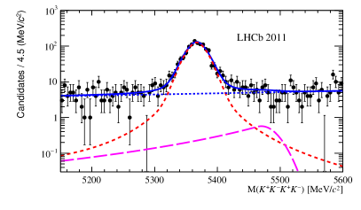
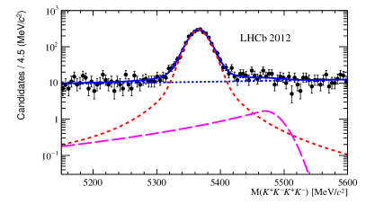
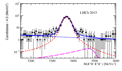
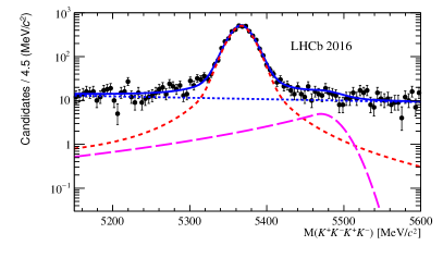
Figure 1: A fit to the four-kaon mass for the (top left) 2011, (top right) 2012, (bottom left) 2015 and (bottom right) 2016 data sets, which are represented by the black points. Also shown are the results of the total fit (blue solid line), with the ${{B}^{0}_{s}}\!\rightarrow\phi\phi$ (red dashed), the ${{\mathchar 28931\relax}^{0}_{b}}\rightarrow\phi{p}{{K}^{-}}$ (magenta long dashed), and the combinatorial (blue short dashed) fit components.

4 Formalism

The final state of the ${{B}^{0}_{s}}\!\rightarrow\phi\phi$ decay comprises a mixture of $C\!P$ eigenstates, which are disentangled by means of an angular analysis in the helicity basis. In this basis, the decay is described by three angles, $\theta_{1}$, $\theta_{2}$ and $\phi$, defined in Fig. 2.

Figure 2: Decay angles for the ${{B}^{0}_{s}}\rightarrow\phi\phi$ decay, where $\theta_{1,2}$ is the angle between the $K^{+}$ momentum in the $\phi_{1,2}$ meson rest frame and the $\phi_{1,2}$ momentum in the ${B}^{0}_{s}$ rest frame, $\Phi$ is the angle between the two $\phi$ meson decay planes and $\hat{n}_{V_{1,2}}$ is the unit vector normal to the decay plane of the $\phi_{1,2}$ meson.

4.1 Decay-time-dependent model

As discussed in Sec. 1, the ${{B}^{0}_{s}}\!\rightarrow\phi\phi$ decay is a $P\rightarrow VV$ decay. However, due to the proximity of the $\phi$ resonance to the scalar $f_{0}(980)$ resonance, there are irreducible contributions to the four-kaon mass spectrum from $P\rightarrow V\kern-1.00006ptS$ ($S$-wave) and $P\rightarrow S\kern-1.00006ptS$ (double $S$-wave) processes, where $S$ denotes a scalar meson, or a nonresonant pair of kaons. Thus, the total amplitude is a coherent sum of $P$-, $S$-, and double $S$-wave processes, and is modelled by making use of the different dependence on the helicity angles associated with these terms, where the helicity angles are defined in Fig. 2. A randomised choice is made for which $\phi$ meson is used to determine $\theta_{1}$ and which is used to determine $\theta_{2}$. The total amplitude ($\mathcal{A}$) containing the $P$-, $S$-, and double $S$-wave components as a function of time, $t$, can be written as [44]

$$\mathcal{A}(t,\theta_{1},\theta_{2},\Phi) =A_{0}(t)\cos\theta_{1}\cos\theta_{2}+\frac{A_{\parallel}(t)}{\sqrt{2}}\sin\theta_{1}\sin\theta_{2}\cos\Phi$$

$$+i\frac{A_{\perp}(t)}{\sqrt{2}}\sin\theta_{1}\sin\theta_{2}\sin\Phi+\frac{A_{S}(t)}{\sqrt{3}}(\cos\theta_{1}+\cos\theta_{2})+\frac{A_{SS}(t)}{3},$$ (1)

where $A_{0}$, $A_{\parallel}$, and $A_{\perp}$ are the $C\!P$-even longitudinal, $C\!P$-even parallel, and $C\!P$-odd perpendicular polarisations of the ${{B}^{0}_{s}}\!\rightarrow\phi\phi$ decay. The $P\rightarrow V\kern-1.00006ptS$ and $P\rightarrow S\kern-1.00006ptS$ processes are described by the $A_{S}$ and $A_{SS}$ amplitudes, respectively, where $P\rightarrow V\kern-1.00006ptS$ is $C\!P$-odd and $P\rightarrow S\kern-1.00006ptS$ is $C\!P$-even. The resulting differential decay rate is proportional to the square of the total amplitude and consists of 15 terms [44]

$$\frac{\mathrm{d}\Gamma}{\mathrm{d}t\,\mathrm{d}\cos\theta_{1}\,\mathrm{d}\cos\theta_{2}\,\mathrm{d}\Phi}\propto|\mathcal{A}(t,\theta_{1},\theta_{2},\Phi)|^{2}=\frac{1}{4}\sum_{i=1}^{15}K_{i}(t)f_{i}(\theta_{1},\theta_{2},\Phi),$$ (2)

where the $f_{i}$ terms are functions of the angular variables and the time-dependence is contained in

$$K_{i}(t)=N_{i}e^{-{\Gamma_{{s}}}t}\left[a_{i}\cosh\left(\frac{1}{2}{\Delta\Gamma_{{s}}}t\right)+b_{i}\sinh\left(\frac{1}{2}{\Delta\Gamma_{{s}}}t\right)+c_{i}\cos({\Delta m_{{s}}}t)+d_{i}\sin({\Delta m_{{s}}}t)\right]\kern-2.5pt.$$ (3)

The coefficients $N_{i},a_{i},b_{i},c_{i}$ and $d_{i}$, which are functions of the $C\!P$ observables, are defined in Appendix A. ${\Delta\Gamma_{{s}}}\equiv\Gamma_{\rm L}-\Gamma_{\rm H}$ is the decay-width difference between the light and heavy ${B}^{0}_{s}$ mass eigenstates, ${\Gamma_{{s}}}\equiv(\Gamma_{\rm L}+\Gamma_{\rm H})/2$ is the average decay width, and ${\Delta m_{{s}}}$ is the ${B}^{0}_{s}$-${\kern 1.79993pt\overline{\kern-1.79993ptB}}{}^{0}_{s}$ oscillation frequency. The differential decay rate for a ${\kern 1.79993pt\overline{\kern-1.79993ptB}}{}^{0}_{s}$ meson produced at $t=0$ is obtained by changing the sign of the $c_{i}$ and $d_{i}$ coefficients. The amplitudes of helicity state $k$ are expressed as

$$A_{k}(t)=|A_{k}|e^{i\delta_{k}}\left(g_{+}(t)+\eta_{k}|\lambda_{k}|e^{-i\phi_{s,k}}g_{-}(t)\right),$$ (4)

where $g_{+}(t)$ and $g_{-}(t)$ describe the time evolution of ${B}^{0}_{s}$ and ${\kern 1.79993pt\overline{\kern-1.79993ptB}}{}^{0}_{s}$ mesons, respectively. $C\!P$ violation is parameterised through

$$\frac{q}{p}\frac{\bar{A}_{k}}{A_{k}}=\eta_{k}|\lambda_{k}|e^{-i\phi_{s,k}}.$$ (5)

where, $q$ and $p$ relate the light and heavy mass eigenstates to the flavour eigenstates and $\eta_{k}$ is the $C\!P$ eigenvalue of the polarisation being considered. Defining the amplitude in this way leads to the forms of $N_{i},a_{i},b_{i},c_{i}$ and $d_{i}$, listed in Table 7 (Appendix A). The $C\!P$-violating asymmetry in ${B}^{0}_{s}$ mixing, which can be characterised by the semileptonic asymmetry, $a_{\mathrm{sl}}^{s}$ is small [45]. Thus, to good approximation $|q/p|=1$, and $|\lambda_{k}|$ quantifies the level of $C\!P$ violation in the decay. 
 Two different fit configurations are performed, one in which the $C\!P$-violation parameters are assumed to be helicity independent and the other in which $C\!P$-violation parameters are allowed to differ as a function of helicity. The helicity independent fit assumes one $C\!P$-violating phase, $\phi_{{s}}^{{{s}{\overline{s}}}{s}}$, which takes the place of all $\phi_{s,k}$ contained in the coefficients of Appendix A, and likewise one parameter that describes direct $C\!P$ violation, $|\lambda|$, which takes the place of all $\lambda_{k}$ coefficients. Due to the small sample size, the number of degrees of freedom is reduced for the case of the helicity-dependent $C\!P$-violation fit. This involves assuming $C\!P$ conservation for the case of the direct $C\!P$-violation parameters, $\lambda=1$, and also for the phase of the longitudinal polarisation, $\phi_{s,0}^{s\bar{s}s}=0$. The longitudinal polarisation has been theoretically calculated as close to zero in the ${{B}^{0}_{s}}\!\rightarrow\phi\phi$ decay [1].

The $\phi_{{s}}^{{{s}{\overline{s}}}{s}}$ and $|\lambda|$ parameters are measured with respect to contributions with the same flavour content as the $\phi$ meson, i.e. ${s}{\overline{s}}$. Regarding the $S$-wave and double $S$-wave terms, the impact of the non-${s}{\overline{s}}$ component of the $\phi$ wavefunction is negligible in this analysis.

4.2 Triple-product asymmetries

Scalar triple products of three-momentum or spin vectors are odd under time reversal,  $T$. Nonzero asymmetries for these observables can either be due to a CP-violating phase or from CP-conserving strong final-state interactions. Four-body final states give rise to three independent momentum vectors in the rest frame of the decaying ${B}^{0}_{s}$ meson. For a detailed review of the phenomenology the reader is referred to Ref. [11].

Two triple products can be defined:

$$\sin\Phi=(\hat{n}_{V_{1}}\times\hat{n}_{V_{2}})\cdot\hat{p}_{V_{1}},$$ (6)

$$\sin 2\Phi=2(\hat{n}_{V_{1}}\cdot\hat{n}_{V_{2}})(\hat{n}_{V_{1}}\times\hat{n}_{V_{2}})\cdot\hat{p}_{V_{1}},$$ (7)

where $\hat{n}_{V_{i}}$ ($i=1,2$) is a unit vector perpendicular to the vector meson ($V_{i}$) decay plane and $\hat{p}_{V_{1}}$ is a unit vector in the direction of $V_{1}$ in the ${B}^{0}_{s}$ rest frame, defined in Fig. 2. This then provides a method of probing $C\!P$ violation without the need to measure the decay time or the initial flavour of the ${B}^{0}_{s}$ meson. It should be noted, that while the observation of nonzero triple-product asymmetries implies $C\!P$ violation or final-state interactions (in the case of ${B}^{0}_{s}$ meson decays), measurements of triple-product asymmetries consistent with zero do not rule out the presence of $C\!P$-violating effects, as the size of the asymmetry also depends on the differences between the strong phases [11].

In the ${{B}^{0}_{s}}\!\rightarrow\phi\phi$ decay, two triple products are defined as $U\equiv\sin\Phi\cos\Phi$ and $V\equiv\sin(\pm\Phi)$ where the positive sign is taken if $\cos\theta_{1}\cos\theta_{2}\geq 0$ and the negative sign otherwise [11]. The $T$-odd asymmetry corresponding to the $U$ observable, $A_{U}$, is defined as the normalised difference between the number of decays with positive and negative values of $\sin\Phi\cos\Phi$,

$$A_{U}\equiv\frac{\Gamma(U>0)-\Gamma(U<0)}{\Gamma(U>0)+\Gamma(U<0)}\propto\int^{\infty}_{0}\Im\left(A_{\perp}(t)A_{\parallel}^{*}(t)+\bar{A}_{\perp}(t)\bar{A}_{\parallel}^{*}(t)\right)\mathrm{d}t.$$ (8)

Similarly, $A_{V}$ is defined as

$$A_{V}\equiv\frac{\Gamma(V>0)-\Gamma(V<0)}{\Gamma(V>0)+\Gamma(V<0)}\propto\int^{\infty}_{0}{\Im}\left(A_{\perp}(t)A_{0}^{*}(t)+\bar{A}_{\perp}(t)\bar{A}_{0}^{*}(t)\right)\mathrm{d}t.$$ (9)

Here, $A_{\perp}$, $A_{\parallel}$ and $A_{0}$ correspond to the three transversity amplitudes. The determination of the triple-product asymmetries is then reduced to a simple counting experiment. Comparing these formulae with Eq. 3 and Appendix A it can be seen that the triple products are related to the $K_{4}(t)$ and $K_{6}(t)$ terms in the decay amplitude.

5 Decay-time resolution

The sensitivity to $\phi_{{s}}^{{{s}{\overline{s}}}{s}}$ is affected by the accuracy of the measured decay time. In order to resolve the fast ${B}^{0}_{s}$-${\kern 1.79993pt\overline{\kern-1.79993ptB}}{}^{0}_{s}$ oscillations, it is necessary to have a decay-time resolution that is much smaller than the oscillation period. To account for the resolution of the measured decay-time distribution, all decay-time-dependent terms are convolved with a Gaussian function, with width $\sigma^{t}_{i}$ that is estimated for each candidate, $i$, based upon the uncertainty obtained from the vertex and kinematic fit [46].

In order to apply a candidate-dependent resolution model during fitting, the estimated per-event decay time uncertainty is needed. This is calibrated using the fact the decay time resolution for the ${{B}^{0}_{s}}\!\rightarrow\phi\phi$ mode is dominated by the secondary vertex resolution. A sample of good-quality tracks, which originate from the primary interaction vertex is selected. Due to the small opening angle of the kaons in the decay of a $\phi$ meson, it is sufficient to use a single prompt track and assign it the mass of a $\phi$ meson. When combining this with another pair of tracks, the invariant mass of the three-body combination is required to be within 250 $\text{\,Me\kern-1.00006ptV\!/}c^{2}$ of the known ${B}^{0}_{s}$ mass. That the decay-time resolution of the signal ${B}^{0}_{s}$ decays can be described well using three tracks has been validated using simulation.

A linear function is then fitted to the distribution of $\sigma^{t}_{i}$ versus $\sigma_{\rm true}^{t}$, with parameters $q_{0}$ and $q_{1}$. Here, $\sigma_{\rm true}^{t}$ denotes the difference between reconstructed decay time and the exact decay time of simulated signal. The per-event decay-time uncertainty used in the decay-time-dependent fit is then calculated as $\sigma^{\rm cal}_{i}=q_{0}+q_{1}\sigma^{t}_{i}$. Gaussian constraints are used to account for the uncertainties on the calibration parameters in the decay-time-dependent fit. The effective single-Gaussian decay-time resolution is found to be between 41 and 44 fs, depending on the data-taking year, in agreement with the expectation from the simulation.

6 Acceptances

The ${{B}^{0}_{s}}\!\rightarrow\phi\phi$ differential decay rate depends on the decay time and three helicity angles as shown in Eq. 2. Good understanding of the efficiencies in these variables is required. The decay-time and angular acceptances are assumed to factorise. Control channels show this assumption has a negligible systematic uncertainty on the physics parameters.

6.1 Angular acceptance

The geometry of the LHCb detector and the momentum requirements imposed on the final-state particles introduce distortions of the helicity angles, giving rise to acceptance effects. Simulated signal events, selected with the same criteria as those applied to data are used to determine these efficiency corrections. The angular acceptances as a function of the three helicity angles are shown in Fig. 3.

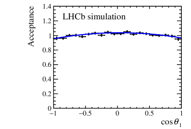
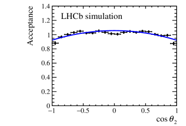
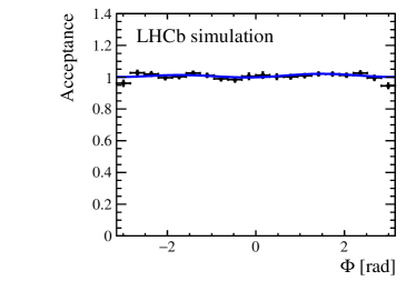
Figure 3: Angular acceptance normalised to the average obtained using simulated ${{B}^{0}_{s}}\!\rightarrow\phi\phi$ decays (top-left) integrated over $\cos\theta_{2}$ and $\Phi$ as a function of $\cos\theta_{1}$, (top-right) integrated over $\cos\theta_{1}$ and $\Phi$ as a function of $\cos\theta_{2}$, and (bottom) integrated over $\cos\theta_{1}$ and $\cos\theta_{2}$ as a function of $\Phi$. Each figure includes the resulting fit curve.

The efficiency is parameterised in terms of the decay angles as

$$\epsilon(\Omega)=\sum_{i,j,k}c_{ijk}P_{i}(\cos\theta_{1})Y_{jk}(\cos\theta_{2},\Phi),$$ (10)

where $\Omega$ depends on the decay angles, $\cos\theta_{1}$, $\cos\theta_{2}$ and $\phi$, the $c_{ijk}$ are coefficients, $P_{i}(\cos\theta_{1})$ are Legendre polynomials, and $Y_{jk}(\cos\theta_{2},\Phi)$ are spherical harmonics. The procedure followed to calculate the coefficients is described in detail in Ref. [47] and exploits the orthogonality of Legendre polynomials. The coefficients are given by

$$c_{ijk}\equiv(j+1/2)\int d\Omega P_{i}(\cos\theta_{1})Y_{jk}(\cos\theta_{2},\Phi)\epsilon(\Omega).$$ (11)

This integral is calculated by means of a Monte Carlo technique, which reduces the integral to a sum over the number of accepted simulated events ($N^{\rm obs}$)

$$c_{ijk}\propto(j+1/2)\frac{1}{N^{\rm obs}}\sum_{e=1}^{N^{\rm obs}}\frac{P_{i}(\cos\theta_{1,e})Y_{jk}(\cos\theta_{2,e},\Phi_{e})}{P^{\rm gen}(\Omega_{e}|t_{e})},$$ (12)

where $P^{\rm gen}$ is the probability density function (PDF) without acceptance where the parameters are set to values used in the Monte Carlo generation. In order to easily incorporate the angular acceptance, it is convenient to write angular functions of Eq. 2 in the same basis as the efficiency parameterisation, i.e.

$$f_{a}(\cos\theta_{1},\cos\theta_{2},\Phi)=\sum_{ijkl}\kappa_{ijkl,a}P_{ij}(\cos\theta_{1})Y_{kl}(\cos\theta_{2},\Phi),$$ (13)

where $P_{ij}(\cos\theta_{1})$ are the associated Legendre polynomials, $\kappa_{ijkl,a}$ are coefficients and $a$ numerates the 15 terms outlined earlier. The parameterisation for each angular function is given in Table 1.

The normalisation of the angular component in the decay-time dependent fit occurs through the 15 integrals $\zeta_{k}=\int\epsilon(\Omega)f_{k}(\Omega)\mathrm{d}\Omega$, where $\epsilon(\Omega)$ is the efficiency as a function of the helicity angles as shown in Eq. 10 and $f_{k}(\Omega)$ are the angular functions as defined in Eq. 13.

Table 1: Angular coefficients, written in the same basis as the efficiency parameterisation.

$\scriptsize\begin{array}[]{c|c|c}i&f_{i}\,\mathrm{in}P_{i\,j}Y_{k\,l}\,{\rm basis}&f_{i}\\ \hline\cr 1&8/9P_{00}Y_{00}+16/9/\sqrt{5}P_{00}Y_{20}+16/9P_{20}Y_{00}+32/(9\sqrt{5})P_{20}Y_{20}&4\cos^{2}\theta_{1}\cos^{2}\theta_{2}\\ \hline\cr 2&8/9P_{00}Y_{00}-8/9P_{00}Y_{20}-8/9\sqrt{5}P_{20}Y_{00}+8/(9\sqrt{5})P_{20}Y_{20}+(2/9)\sqrt{12/5}P_{22}Y_{22}&\sin^{2}\theta_{1}\sin^{2}\theta_{2}(1{+}\cos 2\Phi)\\ \hline\cr 3&8/9P_{00}Y_{00}-8/9P_{00}Y_{20}-8/9\sqrt{5}P_{20}Y_{00}+8/(9\sqrt{5})P_{20}Y_{20}-(2/9)\sqrt{12/5}P_{22}Y_{22}&\sin^{2}\theta_{1}\sin^{2}\theta_{2}(1{-}\cos 2\Phi)\\ \hline\cr 4&-8/9\sqrt{3/5}P_{2,2}Y_{2,-2}&-2\sin^{2}\theta_{1}\sin^{2}\theta_{2}\sin 2\Phi\\ \hline\cr 5&8/9\sqrt{6/5}P_{2,1}Y_{2,1}&\sqrt{2}\sin 2\theta_{1}\sin 2\theta_{2}\cos\Phi\\ \hline\cr 6&-8/9\sqrt{6/5}P_{2,1}Y_{2,1}&-\sqrt{2}\sin 2\theta_{1}\sin 2\theta_{2}\sin\Phi\\ \hline\cr 7&(8/9)P_{00}Y_{00}&\frac{4}{9}\\ \hline\cr 8&16/9P_{00}Y_{00}+16/9/\sqrt{5}P_{00}Y_{20}+16/9P_{20}Y{00}+16\sqrt{3}/9P_{10}Y_{10}&\frac{4}{3}(\cos\theta_{1}+\cos\theta_{2})^{2}\\ \hline\cr 9&16\sqrt{3}/2P_{10}Y_{00}+16/9P_{00}Y_{10}&\frac{8}{3\sqrt{3}}(\cos\theta_{1}+\cos\theta_{2})\\ \hline\cr 10&16/(3\sqrt{3})P_{10}Y_{10}&\frac{8}{3}\cos\theta_{1}\cos\theta_{2}\\ \hline\cr 11&(8/9)\sqrt{6}P_{11}Y_{11}&\frac{4\sqrt{2}}{3}\sin\theta_{1}\sin\theta_{2}\cos\Phi\\ \hline\cr 12&(8/9)\sqrt{6}P_{11}Y_{1-1}&-\frac{4\sqrt{2}}{3}\sin\theta_{1}\sin\theta_{2}\sin\Phi\\ \hline\cr 13&16\sqrt{3}/9P_{10}Y_{00}+16/9P_{00}Y_{10}+32/9P_{20}Y{10}+32/(9\sqrt{5})P_{20}Y_{20}&\begin{array}[]{c}\frac{8}{\sqrt{3}}\cos\theta_{1}\cos\theta_{2}\\ \times(\cos\theta_{1}+\cos\theta_{2})\end{array}\\ \hline\cr 14&(8/9)\sqrt{2/3}P_{21}Y_{11}+(24/9)\sqrt{2/15}P_{11}Y_{21}&\begin{array}[]{c}\frac{4\sqrt{2}}{\sqrt{3}}\sin\theta_{1}\sin\theta_{2}\\ \times(\cos\theta_{1}+\cos\theta_{2})\cos\Phi\end{array}\\ \hline\cr 15&-(8/9)\sqrt{2/3}P_{21}Y_{1-1}-(24/9)\sqrt{2/15}P_{11}Y_{2-1}&\begin{array}[]{c}-\frac{4\sqrt{2}}{3}\sin\theta_{1}\sin\theta_{2}\\ \times(\cos\theta_{1}+\cos\theta_{2})\sin\Phi\end{array}\\ \end{array}$

The angular acceptance is calculated correcting for the differences in kinematic variables between data and simulation. This includes differences in the MLP training variables that can affect acceptance corrections through correlations with the helicity angles.

The fit to determine the triple-product asymmetries assumes that the $U$ and $V$ observables are symmetric in the acceptance corrections. Simulation is used to assign a systematic uncertainty related to this assumption.

6.2 Decay-time acceptance

The impact-parameter requirements on the final-state particles efficiently suppress the background from the numerous pions and kaons originating from the PV, but introduce a decay-time dependence in the selection efficiency.

The efficiency as a function of the decay time is taken from the ${{B}^{0}_{s}}\rightarrow{{D}^{-}_{s}}(\rightarrow{{K}^{+}}{{K}^{-}}{{\pi}^{-}}){{\pi}^{+}}$ decay, in the case of data taken between 2011 and 2012, and from the ${{B}^{0}}\rightarrow{{J\mskip-3.0mu/\mskip-2.0mu\psi\mskip 2.0mu}}(\rightarrow{\mu^{+}}{\mu^{-}}){{K}^{*0}}(\rightarrow{{K}^{+}}{{\pi}^{-}})$ decay in the case of data taken between 2015 and 2016. The reason for the change in control channel is related to changes to the software-trigger selection between the two data-taking periods. The decay-time acceptances of the control modes are weighted by a multivariate algorithm based on simulated kinematic and topological information, in order to match more closely those of the signal ${{B}^{0}_{s}}\!\rightarrow\phi\phi$ decay.

Cubic splines are used to model the acceptance as a function of decay time in the PDF. The PDF can then be computed analytically with the inclusion of the decay-time acceptance following Ref. [48]. Example decay-time acceptances are shown for the case of the ${{B}^{0}_{s}}\rightarrow{{D}^{-}_{s}}{{\pi}^{+}}$ and ${{B}^{0}}\rightarrow{{J\mskip-3.0mu/\mskip-2.0mu\psi\mskip 2.0mu}}{{K}^{*0}}$ decays in Fig. 4.

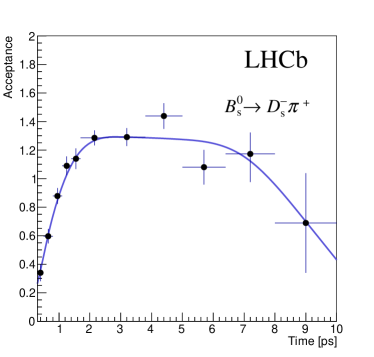
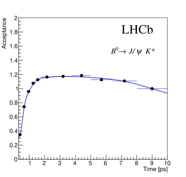
Figure 4: Decay-time acceptances calculated from (left) ${{B}^{0}_{s}}\rightarrow{{D}^{-}_{s}}{{\pi}^{+}}$ decays to match Run 1 data and (right) ${{B}^{0}}\rightarrow{{J\mskip-3.0mu/\mskip-2.0mu\psi\mskip 2.0mu}}{{K}^{*0}}$ decays to match Run 2 data. Superimposed is a parameterisation using cubic splines..

To simplify the measurement of the triple-product asymmetries, the decay-time acceptance is not applied in the fit to determine the triple-product asymmetries. The time acceptance correction has an impact on the asymmetry of 0.3$\%$ and is treated as a source of systematic uncertainty, as further described in Sec. 9.3.

7 Flavour tagging

To obtain sensitivity to $\phi_{{s}}^{{{s}{\overline{s}}}{s}}$, the flavour of the ${B}^{0}_{s}$ meson at production must be determined. At LHCb, tagging is achieved through the use of various algorithms described in Refs.[49, 50]. With these algorithms, the flavour-tagging power, defined as $\epsilon_{\rm tag}\mathcal{D}^{2}$ can be evaluated. Here, $\epsilon_{\rm tag}$ is the flavour-tagging efficiency defined as the fraction of candidates with a flavour tag with respect to the total, and $\mathcal{D}\equiv(1-2\omega)$ is the dilution, where $\omega$ is the average fraction of candidates with an incorrect flavour assignment. This analysis uses opposite-side (OS) and same-side kaon (SSK) flavour taggers.

The OS flavour-tagging algorithm [49] makes use of the $\overline{b}$ ($b$) hadron produced in association with the signal $b$ ($\overline{b}$) hadron. In this analysis, the predicted probability of an incorrect flavour assignment, $\omega$, is determined for each candidate by a neural network that is calibrated using ${{B}^{+}}\rightarrow{{J\mskip-3.0mu/\mskip-2.0mu\psi\mskip 2.0mu}}{{K}^{+}}$, ${{B}^{+}}\rightarrow{{\kern 1.79993pt\overline{\kern-1.79993ptD}}{}^{0}}{{\pi}^{+}}$, ${{B}^{0}}\rightarrow{{J\mskip-3.0mu/\mskip-2.0mu\psi\mskip 2.0mu}}{{K}^{*0}}$, ${{B}^{0}}\rightarrow{{D}^{*-}}{\mu^{+}}{{\nu}_{\mu}}$, and ${{B}^{0}_{s}}\rightarrow{{D}^{-}_{s}}{{\pi}^{+}}$ data as control modes. Details of the calibration procedure can be found in Ref. [51].

When a signal ${B}^{0}_{s}$ meson is formed, there is an associated $\overline{s}$ quark formed in the first branches of the fragmentation that about 50 % of the time forms a charged kaon, which is likely to originate close to the ${B}^{0}_{s}$ meson production point. The kaon charge therefore allows for the identification of the flavour of the signal ${B}^{0}_{s}$ meson. This principle is exploited by the SSK flavour-tagging algorithm [50], which is calibrated with the ${{B}^{0}_{s}}\rightarrow{{D}^{-}_{s}}{{\pi}^{+}}$ decay mode. A neural network is used to select fragmentation particles, improving the flavour-tagging power quoted in the previous decay-time-dependent measurement [10].

Table 2 shows the tagging power for the candidates tagged by only one of the algorithms and those tagged by both. Uncertainties due to the calibration of the flavour tagging algorithms are applied as Gaussian constraints in the decay-time-dependent fit. The initial flavour of the ${B}^{0}_{s}$ meson established from flavour tagging is accounted for during fitting.

Table 2: Tagging performance of the opposite-side (OS) and same-side kaon (SSK) flavour taggers for the ${{B}^{0}_{s}}\!\rightarrow\phi\phi$ decay.

Category	$\varepsilon$ (%)	$\mathcal{D}^{2}$	$\varepsilon\mathcal{D}^{2}$ (%)
OS-only	$12.5$	$0.10$	$1.24\pm 0.10$
SSK-only	$41.0$	$0.04$	$1.74\pm 0.36$
OS&SSK	$23.3$	$0.12$	$2.76\pm 0.20$
Total	$76.8$	$0.08$	$5.74\pm 0.43$

8 Decay-time-dependent measurement

8.1 Likelihood fit

The fit parameters in the polarisation-independent fit are the $C\!P$ violation parameters, ${\phi_{{s}}^{{{s}{\overline{s}}}{s}}}$ and $|\lambda|$, the squared amplitudes, $|A_{0}|^{2}$, $|A_{\perp}|^{2}$, $|A_{S}|^{2}$, and $|A_{SS}|^{2}$, and the strong phases, $\delta_{\perp}$, $\delta_{\parallel}$, $\delta_{0}$, $\delta_{S}$, and $\delta_{SS}$, as defined in Sec. 4.1. The $P$-wave amplitudes are defined such that $|A_{0}|^{2}+|A_{\perp}|^{2}+|A_{\parallel}|^{2}=1$, hence only two of the three amplitudes are free parameters. This normalisation effectively means the $S$ and $SS$ components are measured relative to the $P$-wave. The polarisation-dependent fit allows for a perpendicular, parallel and longitudinal component of $\phi_{{s}}^{{{s}{\overline{s}}}{s}}$ and $|\lambda|$.

The measurement of the parameters of interest is performed through an unbinned negative log likelihood minimisation. The log-likelihood, $\mathcal{L}$, of each candidate is weighted using the sPlot method [52, 53], to remove partly reconstructed and combinatorial background. The negative log-likelihood then takes the form

$$-\ln\mathcal{L}=-\alpha\sum_{e\in{\rm candidates}}W_{e}\ln(S^{e}_{\rm TD}),$$ (14)

where $W_{e}$ are the signal sPlot weights calculated using the four-kaon invariant mass as the discriminating variable. The correlations between the angular and decay-time variables used in the fit with the four-kaon mass are small enough for this technique to be appropriate. The factor $\alpha=\sum_{e}W_{e}/\sum_{e}W_{e}^{2}$ accounts for the sPlot weights in the determination of the statistical uncertainties. The parameter $S^{e}_{\rm TD}$ is the differential decay rate of Eq. 2, modified to the effects of decay-time and angular acceptance, in addition to the probability of an incorrect flavour tag. Explicitly, this can be written as

$$S^{e}_{\rm TD}=\frac{\sum_{i}s^{e}_{i}(t_{e})f_{i}(\Omega_{e})\epsilon(t_{e})}{\sum_{k}\zeta_{k}\int s_{k}(t)f_{k}(\Omega)\epsilon(t)\mathrm{d}t\,\mathrm{d}\Omega},$$ (15)

where $\zeta_{k}$ are the normalisation integrals used to describe the angular acceptance described in Sec. 6.1 and

$$s^{e}_{i}(t) =N_{i}e^{-{\Gamma_{{s}}}t_{e}}\left[c_{i}q_{e}(1-2\omega_{e})\cos({\Delta m_{{s}}}t_{e})+d_{i}q_{e}(1-2\omega_{e})\sin({\Delta m_{{s}}}t_{e})\right.$$

$$\qquad\left.+a_{i}\cosh\left(\frac{1}{2}{\Delta\Gamma_{{s}}}t_{e}\right)+b_{i}\sinh\left(\frac{1}{2}{\Delta\Gamma_{{s}}}t_{e}\right)\right]\otimes R(\sigma^{\rm cal}_{e},t_{e}).$$ (16)

The calibrated probability of an incorrect flavour assignment is given by $\omega_{e}$, $R$ denotes the Gaussian time-resolution function, and the $\otimes$ denotes a convolution operation. In Eq. 16, $q_{e}=1$ $(-1)$ for a ${B}^{0}_{s}$ (${\kern 1.79993pt\overline{\kern-1.79993ptB}}{}^{0}_{s}$) meson at $t=0$ or $q_{e}=0$ where no flavour-tagging information is assigned. The data samples corresponding to the different years of data taking are assigned independent signal weights, decay-time and angular acceptances, and separate Gaussian constraints are applied to the decay-time resolution parameters, as defined in Sec. 5. The ${B}^{0}_{s}$-${\kern 1.79993pt\overline{\kern-1.79993ptB}}{}^{0}_{s}$ oscillation frequency is constrained to the value measured by LHCb of ${\Delta m_{{s}}}=17.768\pm 0.023\text{\,(stat)}\pm 0.006\text{\,(syst)}\text{\,ps}^{-1}$ [54], with the assumption that the systematic uncertainties are uncorrelated with those of the current measurement. The values of the decay width and decay-width difference are constrained to the current best known values of $\Gamma_{s}=0.6646\pm 0.0020$$\text{\,ps}^{-1}$ and $\Delta\Gamma_{s}=0.086\pm 0.006$$\text{\,ps}^{-1}$ [55].

Correction factors must be applied to each of the $S$-wave and double $S$-wave interference terms in the differential decay width. These factors modulate the sizes of the contributions of the interference terms in the angular PDF due to the different line-shapes of kaon pairs originating from spin-1 and spin-0 configurations. This takes the form of a multiplicative factor for each time a $S$-wave pair of kaons interferes with a $P$-wave pair. Their $K^{+}K^{-}$ invariant-mass parameterisations are denoted by $g(m_{{{K}^{+}}{{K}^{-}}})$ and $h(m_{{{K}^{+}}{{K}^{-}}})$, respectively. The $P$-wave configuration is described by a Breit–Wigner function and the $S$-wave configuration is assumed to be uniform. The correction factors, denoted by $C_{SP}$, are defined in Ref. [51]

$$C_{SP}=\int^{m_{\rm h}}_{m_{\rm l}}g^{*}(m_{{{K}^{+}}{{K}^{-}}})h(m_{{{K}^{+}}{{K}^{-}}})\mathrm{d}m_{{{K}^{+}}{{K}^{-}}},$$ (17)

where $m_{\rm h}$ and $m_{\rm l}$ are the upper and lower edges of the $m_{{{K}^{+}}{{K}^{-}}}$ window and the phase of $C_{SP}$ is absorbed in the measurements of $\delta_{S}-\delta_{\perp}$. The factor $|C_{SP}|$, is calculated to be 0.36. In order to determine systematic uncertainties due to the model dependence of the S-wave, $C_{SP}$ factors are recalculated based on the $S$-wave originating from an $f_{0}(980)$ resonance and incorporating the effects of the $m_{K^{+}K^{-}}$ resolution. These alternative assumptions on the $P$-wave and $S$-wave lineshapes yield a $|C_{SP}|$ value of 0.34, which is found to have a negligible effect on the parameter estimation.

8.2 Results

The resulting parameters are given in Table 3. A polarisation-independent fit is performed to calculate values for ${\phi_{{s}}^{{{s}{\overline{s}}}{s}}}$ and $|\lambda|$. A negligible fraction of $S$-wave and double $S$-wave is observed.

Table 3: Results of the decay-time-dependent, polarisation-independent fit for the $C\!P$-violation fit. Uncertainties shown do not include systematic contributions.

Parameter	Fit result
$\phi_{{s}}^{{{s}{\overline{s}}}{s}}$ [rad]	$-0.073\pm 0.115~{}~{}$
$|\lambda|$	$0.99\pm 0.05$
$|A_{0}|^{2}$	$0.381\pm 0.007$
$|A_{\perp}|^{2}$	$0.290\pm 0.008$
$\delta_{\perp}$ [rad]	$2.82\pm 0.18$
$\delta_{\parallel}$ [rad]	$2.56\pm 0.05$

In addition, the $C\!P$-violating phases are also determined in a polarisation-dependent manner. Due to limited size of data samples, the phases $\phi_{s,\parallel}$ and $\phi_{s,\perp}$ are measured under the assumptions that the longitudinal weak phase is $C\!P$-conserving and that there is no direct $C\!P$ violation. In addition, all $S$-wave and double $S$-wave components of the fit are set to zero. The results of the polarisation dependent fit are shown in Table 4. The results for $|A_{0}|^{2}$, $|A_{\perp}|^{2}$, $\delta_{\perp}$ and $\delta_{\parallel}$ are not shown but are in agreement with the results reported in Table 3.

Table 4: Results of the polarisation-dependent fit for the $C\!P$ violation fit. Uncertainties shown do not include systematic contributions.

Parameter	Fit result
$\phi_{s,\parallel}$ [rad]	$0.014\pm 0.055$
$\phi_{s,\perp}$ [rad]	$0.044\pm 0.059$

The correlation matrices for the two fit configurations are provided in Appendix B. Correlations with such decay-time-dependent measurements depend on the central values of the parameters. No large correlation is expected between the $C\!P$-violating parameters when the central values are consistent with $C\!P$ conservation. The largest correlations are found to be between the different decay amplitudes. Cross-checks are performed on simulated data sets generated with the same yield as observed in data, and with the same physics parameters, to establish that the generated values are recovered without biases.

Figure 5 shows the distributions of the ${B}^{0}_{s}$ decay time and the three helicity angles. Superimposed are the projections of the fit result. The projections include corrections for acceptance effects. Pseudoexperiments were used to confirm that the deviation of the data around $\cos\theta_{2}=\pm 0.5$ from the resulting distribution of the fit is compatible with a statistical fluctuation.

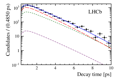
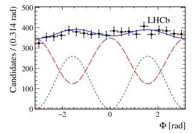
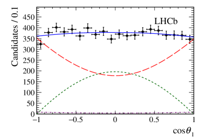
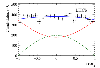
Figure 5: One-dimensional projections of the ${{B}^{0}_{s}}\rightarrow\phi\phi$ fit for (top-left) decay time with binned acceptance, (top-right) helicity angle $\Phi$ and (bottom-left and bottom-right) cosine of the helicity angles $\theta_{1}$ and $\theta_{2}$. The background-subtracted data are marked as black points, while the blue solid lines represent the projections of the fit. The $C\!P$-even $P$-wave, the $C\!P$-odd $P$-wave and the combined $S$-wave and double $S$-wave components are shown by the red long dashed, green short dashed and purple dot-dashed lines, respectively. Fitted components are plotted taking into account efficiencies in the time and angular observables.

8.3 Systematic uncertainties

Various sources of systematic uncertainty are considered in addition to those applied as Gaussian constraints in the fit. These arise from the angular and decay-time acceptances, the mass model used to describe the mass distribution, the determination of the time resolution calibration, and the fit bias. A summary of the systematic uncertainties is given in Table 5.

An uncertainty due to the angular acceptance arises from the choice of weighting scheme described in Sec. 6. This is accounted for by performing multiple alternative weighting schemes for the weighting procedure, based on different kinematic variables in the decay. The largest variation is then assigned as the uncertainty. Further checks are performed to verify that the angular acceptance does not depend on the way in which the event was triggered.

Two sources of systematic uncertainty are considered concerning the decay-time acceptance. These are the statistical uncertainty from the spline coefficients, and also the residual disagreement between the weighted control mode and the signal decay acceptances (see Sec. 6.2). The former is evaluated through fitting the signal data set with 30 different spline functions, whose coefficients are varied according to the corresponding uncertainties. This study is performed with the three different choices of the knot points. The RMS of the fitted parameters is then assigned as the uncertainty. The residual disagreement between the control mode and the signal mode is accounted for with a simulation-based correction. Simplified simulation is used with the corrected acceptance and then fitted with the nominal acceptance. This process is repeated and the resulting bias on the fitted parameters is used as an estimate of the systematic uncertainty.

The uncertainty on the mass model is found by refitting the data with various alternative signal models, consisting of the sum of two Crystal Ball models, the sum of a double-sided Crystal Ball and a Gaussian model. In addition, a Chebyshev polynomial is used to describe the combinatorial background. The signal weights are recalculated and the largest deviation from the nominal fit results is used as the corresponding uncertainty.

Fit biases can arise in maximum-likelihood fits where the number of candidates is small compared to the number of free parameters. The effect of such a bias is taken as a systematic uncertainty which is evaluated by generating and fitting simulated data sets and taking the resulting bias as the uncertainty.

The uncertainties of the effective flavour-tagging power are included in the statistical uncertainty through Gaussian constraints on the calibration parameters, and amount to 10 % of the statistical uncertainty on the $C\!P$-violating phases.

Table 5: Summary of systematic uncertainties (in units of $10^{-2}$) for parameters of interest in the decay-time-dependent measurement.

Parameter	Mass	Angular	Decay-time	Time	Fit	Total
	model	acceptance	acceptance	resolution	bias
$|A_{0}|^{2}$	0.4	1.1	0.1	-	0.2	1.2
$|A_{\perp}|^{2}$	-	0.5	-	-	0.1	0.5
$\delta_{\parallel}$ [rad]	2.7	0.2	0.5	0.1	1.7	3.3
$\delta_{\perp}$ [rad]	3.8	0.3	0.8	1.4	6.0	7.3
$\phi_{{s}}^{{{s}{\overline{s}}}{s}}$ [rad]	1.2	0.5	0.6	2.0	1.1	2.7
$\lambda$	0.5	0.5	0.2	0.3	0.9	1.2
$\phi_{s,\parallel}$ [rad]	0.2	0.2	0.4	0.2	1.0	1.1
$\phi_{s,\perp}$ [rad]	1.4	0.3	0.4	0.3	0.4	1.9

9 Triple-product asymmetries

9.1 Likelihood

To determine the triple-product asymmetries, the data sets are divided according to the sign of the observables $U$ and $V$. Simultaneous likelihood fits to the four-kaon mass distributions are preformed for the $U$ and $V$ variables separately. The set of free parameters in the fits to determine the $U$ and $V$ observables consists of their total yields and the asymmetries $A_{U(V)}$. The mass model is the same as that described in Sec. 3. The total PDF, $D_{\rm TP}$, is then of the form

$$D_{\rm TP}=\sum_{i\in\{+,-\}}\left(f_{i}^{S}G^{S}(m_{{{K}^{+}}{{K}^{-}}{{K}^{+}}{{K}^{-}}})+\sum_{k}f^{k}_{i}P^{k}(m_{{{K}^{+}}{{K}^{-}}{{K}^{+}}{{K}^{-}}})\right),$$ (18)

where $k$ indicates the sum over the background components with corresponding PDFs, $P^{j}$, and $G^{S}$ is the signal PDF, as described in Sec. 3. The parameters $f^{S}_{i}$ found in Eq. 18 are related to the asymmetry, $A_{U(V)}^{S}$, through

$$f_{U(V),+}^{S}=\frac{1}{2}(1+A^{S}_{U(V)}),$$ (19)

$$f_{U(V),-}^{S}=\frac{1}{2}(1-A^{S}_{U(V)}),$$ (20)

where $S$ denotes the signal component of the four-kaon mass fit, as described in Sec. 3. Peaking backgrounds are assumed to be symmetric in $U$ and $V$.

9.2 Results

The triple-product asymmetries found from the simultaneous fit described in Sec. 9.1 are measured separately for the 2015 and 2016 data. The results are combined by performing likelihood scans of the asymmetry parameters and summing the two years. This gives

$A_{U}$ $~{}=~{}$	$-$0.003$\,\,\pm\,$	0.015 ,
$A_{V}$ $~{}=~{}$	$-$0.012$\,\,\pm\,$	0.015 ,

where the uncertainties are statistical only.

9.3 Systematic uncertainties

As for the case of the decay-time-dependent fit, significant contributions to the systematic uncertainty arise from the decay-time and angular acceptances. Minor uncertainties also result from the knowledge of the mass model of the signal and the composition of peaking backgrounds.

The effect of the decay-time acceptance is determined through the generation of simulated samples including the decay-time acceptance and fitted with the method described in Sec. 9.1. The resulting deviation from the nominal fit results is used to assign a systematic uncertainty. The effect of the angular acceptance is evaluated by generating simulated data sets with and without the inclusion of the angular acceptance. The difference between the nominal fit results and the results obtained using the simulated samples including the decay-time acceptance is then used as a systematic uncertainty.

Uncertainties related to the mass model are evaluated using a similar approach to that described in Sec. 8.3. Additional uncertainties arise from the assumption that the peaking background is symmetric in $U$ and $V$. The deviation observed without this assumption is then added as a systematic uncertainty. Similarly, the assumption that the combinatorial background has no asymmetry yields an identical uncertainty. The systematic uncertainties are summarised in Table 6.

Table 6: Summary of systematic uncertainties on $A_{U}$ and $A_{V}$.

Source	Uncertainty
Time acceptance	0.003
Angular acceptance	0.003
Mass model	0.001
Combinatorial background	0.001
Peaking background	0.001
Total	0.005

9.4 Combination of Run 1 and Run 2 results

The Run 2 (2015–2016) values for the triple product asymmetries are

$A_{U}$ $~{}=~{}$	$-$0.003 $\,\,\pm\,$	0.015  (stat) $\pm\,$	0.005  (syst)	,
$A_{V}$ $~{}=~{}$	$-$0.012 $\,\,\pm\,$	0.015  (stat) $\pm\,$	0.005  (syst)	,

whilst the Run 1 (2011–2012) values from Ref. [10] are

$A_{U}$ $~{}=~{}$	$-$0.003 $\,\,\pm\,$	0.017  (stat) $\pm\,$	0.006  (syst)	,
$A_{V}$ $~{}=~{}$	$-$0.017 $\,\,\pm\,$	0.017  (stat) $\pm\,$	0.006  (syst)	.

The Run 1 and Run 2 results are combined by calculating a weighted average. In this procedure the decay-time and angular acceptance systematic uncertainties and peaking backgrounds are assumed to be fully correlated. All other systematic uncertainties are assumed to be uncorrelated. This gives a final result of

$A_{U}$ $~{}=~{}$	$-$0.003$\,\,\pm\,$	0.011 (stat)$\,\,\pm\,$	0.004 (syst),
$A_{V}$ $~{}=~{}$	$-$0.014$\,\,\pm\,$	0.011 (stat)$\,\,\pm\,$	0.004 (syst).

The Run 1 and Run 2 results are compatible with each other, and the asymmetries are consistent with zero. No evidence for $C\!P$ violation is found.

10 Search for the $B^{0}\rightarrow\phi\phi$ decay

The selection criteria for the $B^{0}\rightarrow\phi\phi$ mode are based on the ${{B}^{0}_{s}}\!\rightarrow\phi\phi$ selection, with some modifications. The Punzi figure of merit [42] is used for the ${{B}^{0}}\rightarrow\phi\phi$ search, resulting in a more stringent MLP requirement. Furthermore, the uncertainty on the four-kaon mass is required to be less than 25$\text{\,Me\kern-1.00006ptV\!/}c^{2}$, corresponding to roughly $3\sigma$ separation between the ${{B}^{0}_{s}}$ and $B^{0}$ mass peaks. The ${{B}^{0}_{s}}\!\rightarrow\phi\phi$ decay is used as normalisation decay mode. The signal PDF for the mass of the ${B}^{0}$ meson is assumed to be the same as that of the ${B}^{0}_{s}$ decay, with the modification of the resolution according to a scaling factor, which is defined as

$$\alpha=\frac{m_{B^{0}}-4m_{K}}{m_{B^{0}_{s}}-4m_{K}}=0.974,$$ (21)

where $m_{K}$ is the known ${K}^{+}$ mass.

Figure 6 shows the fit to the full data set. The ${{\mathchar 28931\relax}^{0}_{b}}\rightarrow\phi pK$ contribution is fixed to 109 candidates, following the same method described in Sec. 3. The fit returns a yield of $4.9\pm 9.2$ ${{B}^{0}}\rightarrow\phi\phi$ decays.

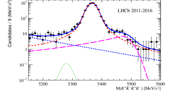
Figure 6: Fit to the four-kaon invariant mass. The total PDF as described in the text is shown as a blue solid line, ${{B}^{0}_{s}}\!\rightarrow\phi\phi$ as a red dashed line, ${{B}^{0}}\rightarrow\phi\phi$ as a green dotted line, the ${{\mathchar 28931\relax}^{0}_{b}}\rightarrow\phi pK$ contribution as a magenta long-dashed line and the combinatorial background as a blue short-dashed line.

The Confidence Levels (${\rm CL}_{s}$) method [56] is used to set a limit on the $B^{0}\rightarrow\phi\phi$ branching fraction. A total of 10,000 pseudoexperiments are used to calculate each point of the scan.

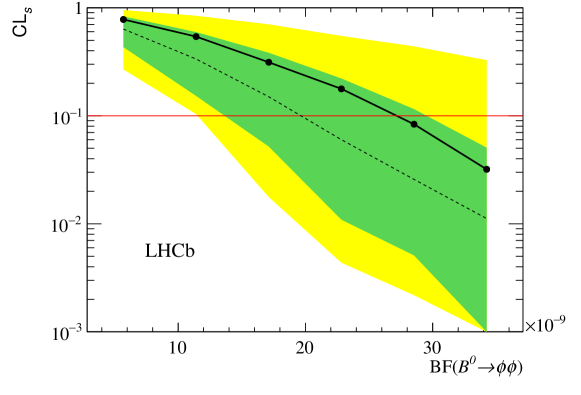
Figure 7: Results of the ${\rm CL}_{s}$ scan as a function of the ${{B}^{0}}\rightarrow\phi\phi$ yield. The solid black line shows the observed ${\rm CL}_{s}$ distribution, while the dotted black line indicates the expected distribution. The green (yellow) band marks the $1\sigma$ ($2\sigma$) confidence region on the expected ${\rm CL}_{s}$. The $90\,\%$ CL limit is shown as a red line.

Figure 7 shows the results of the ${\rm CL}_{s}$ scan. At $90\,\%$ CL, $N_{{{B}^{0}}}<23.7$. These limits are converted to a branching fraction using

$$\mathcal{B}(B^{0}\rightarrow\phi\phi)=N_{B^{0}}\times\frac{\epsilon_{B^{0}\rightarrow\phi\phi}}{\epsilon_{{{B}^{0}_{s}}\!\rightarrow\phi\phi}}\times\frac{\mathcal{B}(B_{s}^{0}\rightarrow\phi\phi)\times f_{s}/f_{d}}{N_{B_{s}^{0}\rightarrow\phi\phi}},$$ (22)

where $N_{{{B}^{0}}}$ is the limit on the $B^{0}\rightarrow\phi\phi$ yield, and $N_{{{B}^{0}_{s}}\!\rightarrow\phi\phi}$ is the $B_{s}^{0}$ yield from the fit displayed in Fig. 6. The relative reconstruction and selection efficiency of the ${{B}^{0}_{s}}\!\rightarrow\phi\phi$ and $B^{0}\rightarrow\phi\phi$ decays, $\epsilon_{B^{0}\rightarrow\phi\phi}/\epsilon_{{{B}^{0}_{s}}\!\rightarrow\phi\phi}$, is determined to be 0.986 using simulation. The ratio of the fragmentation functions has been measured at 7 and 8  TeV to be $f_{s}/f_{d}=0.259\pm 0.015$ within the LHCb acceptance [57]. The production fraction at 13  TeV has been shown to be consistent with that of the 7 and 8  TeV data [58]. The $\mathcal{B}({{B}^{0}_{s}}\!\rightarrow\phi\phi)=(1.84\pm 0.05\text{\,(stat)}\pm 0.07\text{\,(syst)}\pm 0.11(f_{s}/f_{d})\pm 0.12\,(\rm norm))\times 10^{-5}$ branching fraction is an external input taken from Ref. [26]. To set the limit, the uncertainties on the ${{B}^{0}_{s}}\!\rightarrow\phi\phi$ branching fraction are propagated to the limit, where the uncertainty on the ${{B}^{0}_{s}}\!\rightarrow\phi\phi$ branching fraction arising from $f_{s}/f_{d}$ is already included in the uncertainty on the normalisation mode, ${{B}^{0}}\rightarrow\phi{{K}^{*}}$. The maximum value of $\mathcal{B}({{B}^{0}_{s}}\!\rightarrow\phi\phi)$ including the systematic contribution is found to be $1.99\times 10^{-5}$ and is used in Eq. 22. This therefore translates to a limit of

$$\mathcal{B}(B^{0}\rightarrow\phi\phi)<2.7\,(3.0)\times 10^{-8}\,\mathrm{at}\,90\,\%\,(95\,\%)\,{\rm CL},$$

which supersedes the previous best limit.

11 Summary and conclusions

Measurements of $C\!P$ violation in the ${{B}^{0}_{s}}\!\rightarrow\phi\phi$ decay are presented, based on a sample of proton-proton collision data corresponding to an integrated luminosity of 5.0$\text{\,fb}^{-1}$ collected with the LHCb detector. The $C\!P$-violating phase, $\phi_{{s}}^{{{s}{\overline{s}}}{s}}$, and $C\!P$ violation parameter, $|\lambda|$, are determined in a helicity-independent manner to be

$\phi_{{s}}^{{{s}{\overline{s}}}{s}}$ $~{}=~{}$	$-$0.073$\,\,\pm\,$	0.115 (stat)$\,\,\pm\,$	0.027 (syst) $\text{\,rad},$
$|\lambda|$ $~{}=~{}$	0.99$\,\,\pm\,$	0.05 (stat)$\,\,\pm\,$	0.01 (syst) .

The $C\!P$-violating phases are also measured in a polarisation-dependent manner, with the assumption that the longitudinal weak phase is $C\!P$-conserving ($\phi_{s,0}=0$) and that no direct $C\!P$ violation is present ($|\lambda|=1$). The $C\!P$ phases corresponding to the parallel, $\phi_{s,\parallel}$, and perpendicular, $\phi_{s,\perp}$, polarisations are determined to be

$\phi_{s,\parallel}$ $~{}=~{}$	0.014$\,\,\pm\,$	0.055 (stat)$\,\,\pm\,$	0.011 (syst) $\text{\,rad},$
$\phi_{s,\perp}$ $~{}=~{}$	0.044$\,\,\pm\,$	0.059 (stat)$\,\,\pm\,$	0.019 (syst) $\text{\,rad}.$

The results are in agreement with SM predictions [1, 2, 3]. The uncertainties have been validated with simulation. When compared with the $C\!P$-violating phase measured in ${{{B}^{0}_{s}}\rightarrow{{J\mskip-3.0mu/\mskip-2.0mu\psi\mskip 2.0mu}}{{K}^{+}}{{K}^{-}}}$ and ${{{B}^{0}_{s}}\rightarrow{{J\mskip-3.0mu/\mskip-2.0mu\psi\mskip 2.0mu}}{{\pi}^{+}}{{\pi}^{-}}}$ decays [51], these results show that no significant $C\!P$ violation is present either in ${B}^{0}_{s}$-${\kern 1.79993pt\overline{\kern-1.79993ptB}}{}^{0}_{s}$ mixing or in the ${\overline{b}}\rightarrow{\overline{s}}{{s}{\overline{s}}}$ decay amplitude, though the increased precision of the measurement presented in Ref. [51] leads to more stringent constraints on $C\!P$ violation in ${B}^{0}_{s}$-${\kern 1.79993pt\overline{\kern-1.79993ptB}}{}^{0}_{s}$ mixing.

The polarisation amplitudes and strong phases are measured independently of polarisation to be

$|A_{0}|^{2}$ $~{}=~{}$	$0.381$  ±	0.007 (stat) $\,\,\pm\,$	0.012 (syst) ,
$|A_{\perp}|^{2}$ $~{}=~{}$	$0.290$  ±	0.008 (stat) $\,\,\pm\,$	0.007 (syst) ,
$\delta_{\perp}$ $~{}=~{}$	$2.818$  ±	0.178 (stat) $\,\,\pm\,$	0.073 (syst) $\text{\,rad},$
$\delta_{\parallel}$ $~{}=~{}$	$2.559$  ±	0.045 (stat) $\,\,\pm\,$	0.033 (syst) $\text{\,rad}.$

The polarisation amplitudes and strong phases measured in the polarisation-dependent fit are in agreement with the results listed here. In addition, values of the polarisation amplitudes are found to agree well with previous measurements [59, 60, 13, 10] and with predictions from QCD factorisation [2, 3].

The most precise measurements to date of the triple-product asymmetries are determined from a separate time-integrated fit to be

$A_{U}$ $~{}=~{}$	$-$0.003$\,\,\pm\,$	0.011 (stat)$\,\,\pm\,$	0.004 (syst) ,
$A_{V}$ $~{}=~{}$	$-$0.014$\,\,\pm\,$	0.011 (stat)$\,\,\pm\,$	0.004 (syst) ,

in agreement with previous measurements [59, 13, 10]. The measured values of the $C\!P$-violating phase and triple-product asymmetries are consistent with the hypothesis of $C\!P$ conservation in ${\overline{b}}\rightarrow{\overline{s}}{{s}{\overline{s}}}$ transitions.

In addition, the most stringent limit on the branching fraction of the ${{B}^{0}}\rightarrow\phi\phi$ decay is presented and it is found to be

$$\mathcal{B}(B^{0}\rightarrow\phi\phi)<2.7\times 10^{-8}\,\mathrm{at}\,90\,\%\,{\rm CL}.$$

Appendix A Time-dependent terms

In Table 7, $\delta_{S}$ and $\delta_{SS}$ are the strong phases of the $P\rightarrow V\kern-1.00006ptS$ and $P\rightarrow S\kern-1.00006ptS$ processes, respectively. The $P$-wave strong phases are dependent on $\delta_{\parallel}$ and $\delta_{0}$.

Table 7: Coefficients of the time-dependent terms and angular functions used in Eq. 2. Amplitudes are defined at $t=0$.

$i$	$N_{i}$	$a_{i}$	$b_{i}$	$c_{i}$	$d_{i}$	$f_{i}$
$1$	$|A_{0}|^{2}$	$1+|\lambda_{0}|^{2}$	$-2|\lambda_{0}|\cos(\phi)$	$1-|\lambda_{0}|^{2}$	$2|\lambda_{0}|\sin(\phi)$	$4\cos^{2}\theta_{1}\cos^{2}\theta_{2}$
$2$	$|A_{\parallel}|^{2}$	$1+|\lambda_{\parallel}|^{2}$	$-2|\lambda_{\parallel}|\cos(\phi_{s,\parallel})$	$1-|\lambda_{\parallel}|^{2}$	$2|\lambda_{\parallel}|\sin(\phi_{s,\parallel})$	$\sin^{2}\theta_{1}\sin^{2}\theta_{2}(1{+}\cos 2\Phi)$
$3$	$|A_{\perp}|^{2}$	$1+|\lambda_{\perp}|^{2}$	$2|\lambda_{\perp}|\cos(\phi_{s,\perp})$	$1-|\lambda_{\perp}|^{2}$	$-2|\lambda_{\parallel}|\sin(\phi_{s,\perp})$	$\sin^{2}\theta_{1}\sin^{2}\theta_{2}(1{-}\cos 2\Phi)$
$4$	$\frac{|A_{\parallel}||A_{\perp}|}{2}$	$\begin{array}[]{c}\sin(\delta_{\parallel}-\delta_{\perp})-|\lambda_{\parallel}||\lambda_{\perp}|\cdot\\ \sin(\delta_{\parallel}-\delta_{\perp}-\phi_{s,\parallel}+\phi_{s,\perp})\end{array}$	$\begin{array}[]{c}-|\lambda_{\parallel}|\sin(\delta_{\parallel}-\delta_{\perp}-\phi_{s,\parallel})\\ +|\lambda_{\perp}|\sin(\delta_{\parallel}-\delta_{\perp}+\phi_{s,\perp})\end{array}$	$\begin{array}[]{c}\sin(\delta_{\parallel}-\delta_{\perp})+|\lambda_{\parallel}||\lambda_{\perp}|\cdot\\ \sin(\delta_{\parallel}-\delta_{\perp}-\phi_{s,\parallel}+\phi_{s,\perp})\end{array}$	$\begin{array}[]{c}|\lambda_{\parallel}|\cos(\delta_{\parallel}-\delta_{\perp}-\phi_{s,\parallel})\\ +|\lambda_{\perp}|\cos(\delta_{\parallel}-\delta_{\perp}+\phi_{s,\perp})\end{array}$	$-2\sin^{2}\theta_{1}\sin^{2}\theta_{2}\sin 2\Phi$
$5$	$\frac{|A_{\parallel}||A_{0}|}{2}$	$\begin{array}[]{c}\cos(\delta_{\parallel}-\delta_{0})+|\lambda_{\parallel}||\lambda_{0}|\cdot\\ \cos(\delta_{\parallel}-\delta_{0}-\phi_{s,\parallel}+\phi)\end{array}$	$\begin{array}[]{c}-|\lambda_{\parallel}|\cos(\delta_{\parallel}-\delta_{0}-\phi_{s,\parallel})\\ +|\lambda_{0}|\cos(\delta_{\parallel}-\delta_{0}+\phi)\end{array}$	$\begin{array}[]{c}\cos(\delta_{\parallel}-\delta_{0})-|\lambda_{\parallel}||\lambda_{0}|\cdot\\ \sin(\delta_{\parallel}-\delta_{0}-\phi_{s,\parallel}+\phi)\end{array}$	$\begin{array}[]{c}-|\lambda_{\parallel}|\sin(\delta_{\parallel}-\delta_{0}-\phi_{s,\parallel})\\ +|\lambda_{0}|\sin(\delta_{\parallel}-\delta_{0}+\phi)\end{array}$	$\sqrt{2}\sin 2\theta_{1}\sin 2\theta_{2}\cos\Phi$
$6$	$\frac{|A_{0}||A_{\perp}|}{2}$	$\begin{array}[]{c}\sin(\delta_{0}-\delta_{\perp})-|\lambda_{0}||\lambda_{\perp}|\cdot\\ \sin(\delta_{0}-\delta_{\perp}-\phi+\phi_{s,\perp})\end{array}$	$\begin{array}[]{c}-|\lambda_{0}|\sin(\delta_{0}-\delta_{\perp}-\phi)\\ +|\lambda_{\perp}|\sin(\delta_{0}-\delta_{\perp}+\phi_{s,\perp})\end{array}$	$\begin{array}[]{c}\sin(\delta_{0}-\delta_{\perp})+|\lambda_{0}||\lambda_{\perp}|\cdot\\ \sin(\delta_{0}-\delta_{\perp}-\phi+\phi_{s,\perp})\end{array}$	$\begin{array}[]{c}|\lambda_{0}|\cos(\delta_{0}-\delta_{\perp}-\phi)\\ +|\lambda_{\perp}|\cos(\delta_{0}-\delta_{\perp}+\phi_{s,\perp})\end{array}$	$-\sqrt{2}\sin 2\theta_{1}\sin 2\theta_{2}\sin\Phi$
$7$	$|A_{SS}|^{2}$	$1+|\lambda_{ss}|^{2}$	$-2|\lambda_{ss}|\cos(\phi_{s,ss})$	$1-|\lambda_{ss}|^{2}$	$2|\lambda_{ss}|\sin(\phi_{s,ss})$	$\frac{4}{9}$
$8$	$|A_{S}|^{2}$	$1+|\lambda_{s}|^{2}$	$2|\lambda_{s}|\cos(\phi_{s,s})$	$1-|\lambda_{s}|^{2}$	$-2|\lambda_{s}|\sin(\phi_{s,s})$	$\frac{4}{3}(\cos\theta_{1}+\cos\theta_{2})^{2}$
$9$	$\frac{|A_{S}||A_{SS}|}{2}$	$\begin{array}[]{c}\cos(\delta_{s}-\delta_{ss})-|\lambda_{s}||\lambda_{ss}|\cdot\\ \cos(\delta_{s}-\delta_{ss}-\phi_{s,s}+\phi_{s,ss})\end{array}$	$\begin{array}[]{c}|\lambda_{s}|\cos(\delta_{s}-\delta_{ss}-\phi_{s,s})\\ +|\lambda_{ss}|\cos(\delta_{s}-\delta_{ss}+\phi_{s,ss})\end{array}$	$\begin{array}[]{c}\cos(\delta_{s}-\delta_{ss})+|\lambda_{s}||\lambda_{ss}|\cdot\\ \sin(\delta_{s}-\delta_{ss}-\phi_{s,s}+\phi_{s,ss})\end{array}$	$\begin{array}[]{c}|\lambda_{s}|\sin(\delta_{s}-\delta_{ss}-\phi_{s,s})\\ +|\lambda_{ss}|\sin(\delta_{s}-\delta_{ss}+\phi_{s,ss})\end{array}$	$\frac{8}{3\sqrt{3}}(\cos\theta_{1}+\cos\theta_{2})$
$10$	$\frac{|A_{0}||A_{SS}|}{2}$	$\begin{array}[]{c}\cos(\delta_{0}-\delta_{ss})+|\lambda_{0}||\lambda_{ss}|\cdot\\ \cos(\delta_{0}-\delta_{ss}-\phi+\phi_{s,ss})\end{array}$	$\begin{array}[]{c}-|\lambda_{0}|\cos(\delta_{0}-\delta_{ss}-\phi)\\ +|\lambda_{ss}|\cos(\delta_{0}-\delta_{ss}+\phi_{s,ss})\end{array}$	$\begin{array}[]{c}\cos(\delta_{0}-\delta_{ss})-|\lambda_{0}||\lambda_{ss}|\cdot\\ \sin(\delta_{0}-\delta_{ss}-\phi+\phi_{s,ss})\end{array}$	$\begin{array}[]{c}-|\lambda_{0}|\sin(\delta_{0}-\delta_{ss}-\phi)\\ +|\lambda_{ss}|\sin(\delta_{0}-\delta_{ss}+\phi_{s,ss})\end{array}$	$\frac{8}{3}\cos\theta_{1}\cos\theta_{2}$
$11$	$\frac{|A_{\parallel}||A_{SS}|}{2}$	$\begin{array}[]{c}\cos(\delta_{\parallel}-\delta_{ss})+|\lambda_{\parallel}||\lambda_{ss}|\cdot\\ \cos(\delta_{\parallel}-\delta_{ss}-\phi_{s,\parallel}+\phi_{s,ss})\end{array}$	$\begin{array}[]{c}-|\lambda_{\parallel}|\cos(\delta_{\parallel}-\delta_{ss}-\phi_{s,\parallel})\\ +|\lambda_{ss}|\cos(\delta_{\parallel}-\delta_{ss}+\phi_{s,ss})\end{array}$	$\begin{array}[]{c}\cos(\delta_{\parallel}-\delta_{ss})-|\lambda_{\parallel}||\lambda_{ss}|\cdot\\ \sin(\delta_{\parallel}-\delta_{ss}-\phi_{s,\parallel}+\phi_{s,ss})\end{array}$	$\begin{array}[]{c}-|\lambda_{0}|\sin(\delta_{\parallel}-\delta_{ss}-\phi_{s,\parallel})\\ +|\lambda_{ss}|\sin(\delta_{\parallel}-\delta_{ss}+\phi_{s,ss})\end{array}$	$\frac{4\sqrt{2}}{3}\sin\theta_{1}\sin\theta_{2}\cos\Phi$
$12$	$\frac{|A_{\perp}||A_{SS}|}{2}$	$\begin{array}[]{c}\sin(\delta_{\perp}-\delta_{ss})-|\lambda_{\perp}||\lambda_{ss}|\cdot\\ \sin(\delta_{\perp}-\delta_{ss}-\phi_{s,\perp}+\phi_{s,ss})\end{array}$	$\begin{array}[]{c}|\lambda_{\perp}|\sin(\delta_{\perp}-\delta_{ss}-\phi_{s,\perp})\\ -|\lambda_{ss}|\sin(\delta_{\perp}-\delta_{ss}+\phi_{s,ss})\end{array}$	$\begin{array}[]{c}\sin(\delta_{\perp}-\delta_{ss})+|\lambda_{\perp}||\lambda_{ss}|\cdot\\ \sin(\delta_{\perp}-\delta_{ss}-\phi_{s,\perp}+\phi_{s,ss})\end{array}$	$\begin{array}[]{c}-|\lambda_{\perp}|\cos(\delta_{\perp}-\delta_{ss}-\phi_{s,\perp})\\ -|\lambda_{ss}|\cos(\delta_{\perp}-\delta_{ss}+\phi_{s,ss})\end{array}$	$-\frac{4\sqrt{2}}{3}\sin\theta_{1}\sin\theta_{2}\sin\Phi$
$13$	$\frac{|A_{0}||A_{S}|}{2}$	$\begin{array}[]{c}\cos(\delta_{0}-\delta_{s})-|\lambda_{0}||\lambda_{s}|\cdot\\ \cos(\delta_{0}-\delta_{s}-\phi+\phi_{s,s})\end{array}$	$\begin{array}[]{c}-|\lambda_{0}|\cos(\delta_{0}-\delta_{s}-\phi)\\ -|\lambda_{s}|\cos(\delta_{0}-\delta_{s}+\phi_{s,s})\end{array}$	$\begin{array}[]{c}\cos(\delta_{0}-\delta_{s})+|\lambda_{0}||\lambda_{s}|\cdot\\ \sin(\delta_{0}-\delta_{s}-\phi+\phi_{s,s})\end{array}$	$\begin{array}[]{c}-|\lambda_{0}|\sin(\delta_{0}-\delta_{s}-\phi)\\ -|\lambda_{s}|\sin(\delta_{0}-\delta_{ss}+\phi_{s,s})\end{array}$	$\begin{array}[]{c}\frac{8}{\sqrt{3}}\cos\theta_{1}\cos\theta_{2}\\ \times(\cos\theta_{1}+\cos\theta_{2})\end{array}$
$14$	$\frac{|A_{\parallel}||A_{S}|}{2}$	$\begin{array}[]{c}\cos(\delta_{\parallel}-\delta_{s})-|\lambda_{\parallel}||\lambda_{s}|\cdot\\ \cos(\delta_{\parallel}-\delta_{s}-\phi_{s,\parallel}+\phi_{s,s})\end{array}$	$\begin{array}[]{c}-|\lambda_{\parallel}|\cos(\delta_{\parallel}-\delta_{s}-\phi_{s,\parallel})\\ -|\lambda_{s}|\cos(\delta_{\parallel}-\delta_{s}+\phi_{s,s})\end{array}$	$\begin{array}[]{c}\cos(\delta_{\parallel}-\delta_{s})+|\lambda_{\parallel}||\lambda_{s}|\cdot\\ \sin(\delta_{\parallel}-\delta_{s}-\phi_{s,\parallel}+\phi_{s,s})\end{array}$	$\begin{array}[]{c}-|\lambda_{\parallel}|\sin(\delta_{\parallel}-\delta_{s}-\phi_{s,\parallel})\\ -|\lambda_{s}|\sin(\delta_{\parallel}-\delta_{ss}+\phi_{s,s})\end{array}$	$\begin{array}[]{c}\frac{4\sqrt{2}}{\sqrt{3}}\sin\theta_{1}\sin\theta_{2}\\ \times(\cos\theta_{1}+\cos\theta_{2})\cos\Phi\end{array}$
$15$	$\frac{|A_{\perp}||A_{S}|}{2}$	$\begin{array}[]{c}\sin(\delta_{\perp}-\delta_{s})+|\lambda_{\perp}||\lambda_{s}|\cdot\\ \sin(\delta_{\perp}-\delta_{s}-\phi_{s,\perp}+\phi_{s,s})\end{array}$	$\begin{array}[]{c}|\lambda_{\perp}|\sin(\delta_{\perp}-\delta_{s}-\phi_{s,\perp})\\ +|\lambda_{s}|\sin(\delta_{\perp}-\delta_{s}+\phi_{s,s})\end{array}$	$\begin{array}[]{c}\sin(\delta_{\perp}-\delta_{s})-|\lambda_{\perp}||\lambda_{s}|\cdot\\ \sin(\delta_{\perp}-\delta_{s}-\phi_{s,\perp}+\phi_{s,s})\end{array}$	$\begin{array}[]{c}-|\lambda_{\perp}|\cos(\delta_{\perp}-\delta_{s}-\phi_{s,\perp})\\ +|\lambda_{s}|\cos(\delta_{\perp}-\delta_{s}+\phi_{s,s})\end{array}$	$\begin{array}[]{c}-\frac{4\sqrt{2}}{3}\sin\theta_{1}\sin\theta_{2}\\ \times(\cos\theta_{1}+\cos\theta_{2})\sin\Phi\end{array}$

Appendix B Correlation matrices for the time-dependent fits

Table 8: Statistical correlation matrix of the time-dependent fit.

	$\delta_{\parallel}$	$|A_{\perp}|^{2}$	$\delta_{\perp}$	$|A_{0}|^{2}$	$|\lambda|$	$\phi_{{s}}^{{{s}{\overline{s}}}{s}}$
$\delta_{\parallel}$	1.00	0.14	0.13	$-0.03$	$0.02$	$0.01$
$|A_{\perp}|^{2}$		1.00	0.01	$-0.45$	$0.00$	$-0.03$
$\delta_{\perp}$			1.00	$0.00$	$-0.26$	$-0.15$
$|A_{0}|^{2}$				$1.00$	$-0.01$	$0.01$
$|\lambda|$					$1.00$	$-0.05$
${\phi_{{s}}^{{{s}{\overline{s}}}{s}}}$						$1.00$

Table 9: Statistical correlation matrix of the time-dependent fit in which $C\!P$ violation is polarisation dependent.

	$\delta_{\parallel}$	$|A_{\perp}|^{2}$	$\delta_{\perp}$	$|A_{0}|^{2}$	$\phi_{s,\parallel}$	$\phi_{s,\perp}$
$\delta_{\parallel}$	1.00	0.13	0.13	$-0.02$	$0.58$	$0.41$
$|A_{\perp}|^{2}$		1.00	0.03	$-0.45$	$0.00$	$0.01$
$\delta_{\perp}$			1.00	$0.00$	$0.08$	$0.13$
$|A_{0}|^{2}$				$1.00$	$0.00$	$0.01$
$|\lambda|$					$1.00$	$0.71$
${\phi_{{s}}^{{{s}{\overline{s}}}{s}}}$						$1.00$

LHCb collaboration

R. Aaij³⁰, C. Abellán Beteta⁴⁷, B. Adeva⁴⁴, M. Adinolfi⁵¹, C.A. Aidala⁷⁸, Z. Ajaltouni⁸, S. Akar⁶², P. Albicocco²¹, J. Albrecht¹³, F. Alessio⁴⁵, M. Alexander⁵⁶, A. Alfonso Albero⁴³, G. Alkhazov³⁶, P. Alvarez Cartelle⁵⁸, A.A. Alves Jr⁴⁴, S. Amato², Y. Amhis¹⁰, L. An²⁰, L. Anderlini²⁰, G. Andreassi⁴⁶, M. Andreotti¹⁹, J.E. Andrews⁶³, F. Archilli²¹, J. Arnau Romeu⁹, A. Artamonov⁴², M. Artuso⁶⁵, K. Arzymatov⁴⁰, E. Aslanides⁹, M. Atzeni⁴⁷, B. Audurier²⁵, S. Bachmann¹⁵, J.J. Back⁵³, S. Baker⁵⁸, V. Balagura^10,b, W. Baldini^19,45, A. Baranov⁴⁰, R.J. Barlow⁵⁹, S. Barsuk¹⁰, W. Barter⁵⁸, M. Bartolini²², F. Baryshnikov⁷⁴, V. Batozskaya³⁴, B. Batsukh⁶⁵, A. Battig¹³, V. Battista⁴⁶, A. Bay⁴⁶, F. Bedeschi²⁷, I. Bediaga¹, A. Beiter⁶⁵, L.J. Bel³⁰, V. Belavin⁴⁰, S. Belin²⁵, N. Beliy⁴, V. Bellee⁴⁶, K. Belous⁴², I. Belyaev³⁷, G. Bencivenni²¹, E. Ben-Haim¹¹, S. Benson³⁰, S. Beranek¹², A. Berezhnoy³⁸, R. Bernet⁴⁷, D. Berninghoff¹⁵, E. Bertholet¹¹, A. Bertolin²⁶, C. Betancourt⁴⁷, F. Betti^18,e, M.O. Bettler⁵², Ia. Bezshyiko⁴⁷, S. Bhasin⁵¹, J. Bhom³², M.S. Bieker¹³, S. Bifani⁵⁰, P. Billoir¹¹, A. Birnkraut¹³, A. Bizzeti^20,u, M. Bjørn⁶⁰, M.P. Blago⁴⁵, T. Blake⁵³, F. Blanc⁴⁶, S. Blusk⁶⁵, D. Bobulska⁵⁶, V. Bocci²⁹, O. Boente Garcia⁴⁴, T. Boettcher⁶¹, A. Boldyrev⁷⁵, A. Bondar^41,w, N. Bondar³⁶, S. Borghi^59,45, M. Borisyak⁴⁰, M. Borsato¹⁵, M. Boubdir¹², T.J.V. Bowcock⁵⁷, C. Bozzi^19,45, S. Braun¹⁵, A. Brea Rodriguez⁴⁴, M. Brodski⁴⁵, J. Brodzicka³², A. Brossa Gonzalo⁵³, D. Brundu^25,45, E. Buchanan⁵¹, A. Buonaura⁴⁷, C. Burr⁵⁹, A. Bursche²⁵, J.S. Butter³⁰, J. Buytaert⁴⁵, W. Byczynski⁴⁵, S. Cadeddu²⁵, H. Cai⁶⁹, R. Calabrese^19,g, S. Cali²¹, R. Calladine⁵⁰, M. Calvi^23,i, M. Calvo Gomez^43,m, A. Camboni^43,m, P. Campana²¹, D.H. Campora Perez⁴⁵, L. Capriotti^18,e, A. Carbone^18,e, G. Carboni²⁸, R. Cardinale²², A. Cardini²⁵, P. Carniti^23,i, K. Carvalho Akiba², A. Casais Vidal⁴⁴, G. Casse⁵⁷, M. Cattaneo⁴⁵, G. Cavallero²², R. Cenci^27,p, M.G. Chapman⁵¹, M. Charles^11,45, Ph. Charpentier⁴⁵, G. Chatzikonstantinidis⁵⁰, M. Chefdeville⁷, V. Chekalina⁴⁰, C. Chen³, S. Chen²⁵, S.-G. Chitic⁴⁵, V. Chobanova⁴⁴, M. Chrzaszcz⁴⁵, A. Chubykin³⁶, P. Ciambrone²¹, X. Cid Vidal⁴⁴, G. Ciezarek⁴⁵, F. Cindolo¹⁸, P.E.L. Clarke⁵⁵, M. Clemencic⁴⁵, H.V. Cliff⁵², J. Closier⁴⁵, J.L. Cobbledick⁵⁹, V. Coco⁴⁵, J.A.B. Coelho¹⁰, J. Cogan⁹, E. Cogneras⁸, L. Cojocariu³⁵, P. Collins⁴⁵, T. Colombo⁴⁵, A. Comerma-Montells¹⁵, A. Contu²⁵, G. Coombs⁴⁵, S. Coquereau⁴³, G. Corti⁴⁵, C.M. Costa Sobral⁵³, B. Couturier⁴⁵, G.A. Cowan⁵⁵, D.C. Craik⁶¹, A. Crocombe⁵³, M. Cruz Torres¹, R. Currie⁵⁵, C.L. Da Silva⁶⁴, E. Dall’Occo³⁰, J. Dalseno^44,51, C. D’Ambrosio⁴⁵, A. Danilina³⁷, P. d’Argent¹⁵, A. Davis⁵⁹, O. De Aguiar Francisco⁴⁵, K. De Bruyn⁴⁵, S. De Capua⁵⁹, M. De Cian⁴⁶, J.M. De Miranda¹, L. De Paula², M. De Serio^17,d, P. De Simone²¹, J.A. de Vries³⁰, C.T. Dean⁵⁶, W. Dean⁷⁸, D. Decamp⁷, L. Del Buono¹¹, B. Delaney⁵², H.-P. Dembinski¹⁴, M. Demmer¹³, A. Dendek³³, D. Derkach⁷⁵, O. Deschamps⁸, F. Desse¹⁰, F. Dettori²⁵, B. Dey⁶, A. Di Canto⁴⁵, P. Di Nezza²¹, S. Didenko⁷⁴, H. Dijkstra⁴⁵, F. Dordei²⁵, M. Dorigo^27,x, A.C. dos Reis¹, A. Dosil Suárez⁴⁴, L. Douglas⁵⁶, A. Dovbnya⁴⁸, K. Dreimanis⁵⁷, L. Dufour⁴⁵, G. Dujany¹¹, P. Durante⁴⁵, J.M. Durham⁶⁴, D. Dutta⁵⁹, R. Dzhelyadin^42,†, M. Dziewiecki¹⁵, A. Dziurda³², A. Dzyuba³⁶, S. Easo⁵⁴, U. Egede⁵⁸, V. Egorychev³⁷, S. Eidelman^41,w, S. Eisenhardt⁵⁵, U. Eitschberger¹³, R. Ekelhof¹³, S. Ek-In⁴⁶, L. Eklund⁵⁶, S. Ely⁶⁵, A. Ene³⁵, S. Escher¹², S. Esen³⁰, T. Evans⁶², A. Falabella¹⁸, C. Färber⁴⁵, N. Farley⁵⁰, S. Farry⁵⁷, D. Fazzini¹⁰, M. Féo⁴⁵, P. Fernandez Declara⁴⁵, A. Fernandez Prieto⁴⁴, F. Ferrari^18,e, L. Ferreira Lopes⁴⁶, F. Ferreira Rodrigues², S. Ferreres Sole³⁰, M. Ferro-Luzzi⁴⁵, S. Filippov³⁹, R.A. Fini¹⁷, M. Fiorini^19,g, M. Firlej³³, C. Fitzpatrick⁴⁵, T. Fiutowski³³, F. Fleuret^10,b, M. Fontana⁴⁵, F. Fontanelli^22,h, R. Forty⁴⁵, V. Franco Lima⁵⁷, M. Franco Sevilla⁶³, M. Frank⁴⁵, C. Frei⁴⁵, J. Fu^24,q, W. Funk⁴⁵, E. Gabriel⁵⁵, A. Gallas Torreira⁴⁴, D. Galli^18,e, S. Gallorini²⁶, S. Gambetta⁵⁵, Y. Gan³, M. Gandelman², P. Gandini²⁴, Y. Gao³, L.M. Garcia Martin⁷⁷, J. García Pardiñas⁴⁷, B. Garcia Plana⁴⁴, J. Garra Tico⁵², L. Garrido⁴³, D. Gascon⁴³, C. Gaspar⁴⁵, G. Gazzoni⁸, D. Gerick¹⁵, E. Gersabeck⁵⁹, M. Gersabeck⁵⁹, T. Gershon⁵³, D. Gerstel⁹, Ph. Ghez⁷, V. Gibson⁵², A. Gioventù⁴⁴, O.G. Girard⁴⁶, P. Gironella Gironell⁴³, L. Giubega³⁵, K. Gizdov⁵⁵, V.V. Gligorov¹¹, C. Göbel⁶⁷, D. Golubkov³⁷, A. Golutvin^58,74, A. Gomes^1,a, I.V. Gorelov³⁸, C. Gotti^23,i, E. Govorkova³⁰, J.P. Grabowski¹⁵, R. Graciani Diaz⁴³, L.A. Granado Cardoso⁴⁵, E. Graugés⁴³, E. Graverini⁴⁶, G. Graziani²⁰, A. Grecu³⁵, R. Greim³⁰, P. Griffith²⁵, L. Grillo⁵⁹, L. Gruber⁴⁵, B.R. Gruberg Cazon⁶⁰, C. Gu³, E. Gushchin³⁹, A. Guth¹², Yu. Guz^42,45, T. Gys⁴⁵, T. Hadavizadeh⁶⁰, C. Hadjivasiliou⁸, G. Haefeli⁴⁶, C. Haen⁴⁵, S.C. Haines⁵², P.M. Hamilton⁶³, Q. Han⁶, X. Han¹⁵, T.H. Hancock⁶⁰, S. Hansmann-Menzemer¹⁵, N. Harnew⁶⁰, T. Harrison⁵⁷, C. Hasse⁴⁵, M. Hatch⁴⁵, J. He⁴, M. Hecker⁵⁸, K. Heijhoff³⁰, K. Heinicke¹³, A. Heister¹³, K. Hennessy⁵⁷, L. Henry⁷⁷, M. Heß⁷¹, J. Heuel¹², A. Hicheur⁶⁶, R. Hidalgo Charman⁵⁹, D. Hill⁶⁰, M. Hilton⁵⁹, P.H. Hopchev⁴⁶, J. Hu¹⁵, W. Hu⁶, W. Huang⁴, Z.C. Huard⁶², W. Hulsbergen³⁰, T. Humair⁵⁸, M. Hushchyn⁷⁵, D. Hutchcroft⁵⁷, D. Hynds³⁰, P. Ibis¹³, M. Idzik³³, P. Ilten⁵⁰, A. Inglessi³⁶, A. Inyakin⁴², K. Ivshin³⁶, R. Jacobsson⁴⁵, S. Jakobsen⁴⁵, J. Jalocha⁶⁰, E. Jans³⁰, B.K. Jashal⁷⁷, A. Jawahery⁶³, F. Jiang³, M. John⁶⁰, D. Johnson⁴⁵, C.R. Jones⁵², C. Joram⁴⁵, B. Jost⁴⁵, N. Jurik⁶⁰, S. Kandybei⁴⁸, M. Karacson⁴⁵, J.M. Kariuki⁵¹, S. Karodia⁵⁶, N. Kazeev⁷⁵, M. Kecke¹⁵, F. Keizer⁵², M. Kelsey⁶⁵, M. Kenzie⁵², T. Ketel³¹, B. Khanji⁴⁵, A. Kharisova⁷⁶, C. Khurewathanakul⁴⁶, K.E. Kim⁶⁵, T. Kirn¹², V.S. Kirsebom⁴⁶, S. Klaver²¹, K. Klimaszewski³⁴, S. Koliiev⁴⁹, M. Kolpin¹⁵, A. Kondybayeva⁷⁴, A. Konoplyannikov³⁷, P. Kopciewicz³³, R. Kopecna¹⁵, P. Koppenburg³⁰, I. Kostiuk^30,49, O. Kot⁴⁹, S. Kotriakhova³⁶, M. Kozeiha⁸, L. Kravchuk³⁹, M. Kreps⁵³, F. Kress⁵⁸, S. Kretzschmar¹², P. Krokovny^41,w, W. Krupa³³, W. Krzemien³⁴, W. Kucewicz^32,l, M. Kucharczyk³², V. Kudryavtsev^41,w, G.J. Kunde⁶⁴, A.K. Kuonen⁴⁶, T. Kvaratskheliya³⁷, D. Lacarrere⁴⁵, G. Lafferty⁵⁹, A. Lai²⁵, D. Lancierini⁴⁷, G. Lanfranchi²¹, C. Langenbruch¹², T. Latham⁵³, C. Lazzeroni⁵⁰, R. Le Gac⁹, R. Lefèvre⁸, A. Leflat³⁸, F. Lemaitre⁴⁵, O. Leroy⁹, T. Lesiak³², B. Leverington¹⁵, H. Li⁶⁸, P.-R. Li^4,aa, X. Li⁶⁴, Y. Li⁵, Z. Li⁶⁵, X. Liang⁶⁵, T. Likhomanenko⁷³, R. Lindner⁴⁵, F. Lionetto⁴⁷, V. Lisovskyi¹⁰, G. Liu⁶⁸, X. Liu³, D. Loh⁵³, A. Loi²⁵, J. Lomba Castro⁴⁴, I. Longstaff⁵⁶, J.H. Lopes², G. Loustau⁴⁷, G.H. Lovell⁵², D. Lucchesi^26,o, M. Lucio Martinez⁴⁴, Y. Luo³, A. Lupato²⁶, E. Luppi^19,g, O. Lupton⁵³, A. Lusiani²⁷, X. Lyu⁴, F. Machefert¹⁰, F. Maciuc³⁵, V. Macko⁴⁶, P. Mackowiak¹³, S. Maddrell-Mander⁵¹, O. Maev^36,45, A. Maevskiy⁷⁵, K. Maguire⁵⁹, D. Maisuzenko³⁶, M.W. Majewski³³, S. Malde⁶⁰, B. Malecki⁴⁵, A. Malinin⁷³, T. Maltsev^41,w, H. Malygina¹⁵, G. Manca^25,f, G. Mancinelli⁹, D. Marangotto^24,q, J. Maratas^8,v, J.F. Marchand⁷, U. Marconi¹⁸, C. Marin Benito¹⁰, M. Marinangeli⁴⁶, P. Marino⁴⁶, J. Marks¹⁵, P.J. Marshall⁵⁷, G. Martellotti²⁹, L. Martinazzoli⁴⁵, M. Martinelli^45,23,i, D. Martinez Santos⁴⁴, F. Martinez Vidal⁷⁷, A. Massafferri¹, M. Materok¹², R. Matev⁴⁵, A. Mathad⁴⁷, Z. Mathe⁴⁵, V. Matiunin³⁷, C. Matteuzzi²³, K.R. Mattioli⁷⁸, A. Mauri⁴⁷, E. Maurice^10,b, B. Maurin⁴⁶, M. McCann^58,45, L. Mcconnell¹⁶, A. McNab⁵⁹, R. McNulty¹⁶, J.V. Mead⁵⁷, B. Meadows⁶², C. Meaux⁹, N. Meinert⁷¹, D. Melnychuk³⁴, M. Merk³⁰, A. Merli^24,q, E. Michielin²⁶, D.A. Milanes⁷⁰, E. Millard⁵³, M.-N. Minard⁷, O. Mineev³⁷, L. Minzoni^19,g, D.S. Mitzel¹⁵, A. Mödden¹³, A. Mogini¹¹, R.D. Moise⁵⁸, T. Mombächer¹³, I.A. Monroy⁷⁰, S. Monteil⁸, M. Morandin²⁶, G. Morello²¹, M.J. Morello^27,t, J. Moron³³, A.B. Morris⁹, R. Mountain⁶⁵, H. Mu³, F. Muheim⁵⁵, M. Mukherjee⁶, M. Mulder³⁰, D. Müller⁴⁵, J. Müller¹³, K. Müller⁴⁷, V. Müller¹³, C.H. Murphy⁶⁰, D. Murray⁵⁹, P. Naik⁵¹, T. Nakada⁴⁶, R. Nandakumar⁵⁴, A. Nandi⁶⁰, T. Nanut⁴⁶, I. Nasteva², M. Needham⁵⁵, N. Neri^24,q, S. Neubert¹⁵, N. Neufeld⁴⁵, R. Newcombe⁵⁸, T.D. Nguyen⁴⁶, C. Nguyen-Mau^46,n, S. Nieswand¹², R. Niet¹³, N. Nikitin³⁸, N.S. Nolte⁴⁵, A. Oblakowska-Mucha³³, V. Obraztsov⁴², S. Ogilvy⁵⁶, D.P. O’Hanlon¹⁸, R. Oldeman^25,f, C.J.G. Onderwater⁷², J. D. Osborn⁷⁸, A. Ossowska³², J.M. Otalora Goicochea², T. Ovsiannikova³⁷, P. Owen⁴⁷, A. Oyanguren⁷⁷, P.R. Pais⁴⁶, T. Pajero^27,t, A. Palano¹⁷, M. Palutan²¹, G. Panshin⁷⁶, A. Papanestis⁵⁴, M. Pappagallo⁵⁵, L.L. Pappalardo^19,g, W. Parker⁶³, C. Parkes^59,45, G. Passaleva^20,45, A. Pastore¹⁷, M. Patel⁵⁸, C. Patrignani^18,e, A. Pearce⁴⁵, A. Pellegrino³⁰, G. Penso²⁹, M. Pepe Altarelli⁴⁵, S. Perazzini¹⁸, D. Pereima³⁷, P. Perret⁸, L. Pescatore⁴⁶, K. Petridis⁵¹, A. Petrolini^22,h, A. Petrov⁷³, S. Petrucci⁵⁵, M. Petruzzo^24,q, B. Pietrzyk⁷, G. Pietrzyk⁴⁶, M. Pikies³², M. Pili⁶⁰, D. Pinci²⁹, J. Pinzino⁴⁵, F. Pisani⁴⁵, A. Piucci¹⁵, V. Placinta³⁵, S. Playfer⁵⁵, J. Plews⁵⁰, M. Plo Casasus⁴⁴, F. Polci¹¹, M. Poli Lener²¹, M. Poliakova⁶⁵, A. Poluektov⁹, N. Polukhina^74,c, I. Polyakov⁶⁵, E. Polycarpo², G.J. Pomery⁵¹, S. Ponce⁴⁵, A. Popov⁴², D. Popov⁵⁰, S. Poslavskii⁴², K. Prasanth³², E. Price⁵¹, C. Prouve⁴⁴, V. Pugatch⁴⁹, A. Puig Navarro⁴⁷, H. Pullen⁶⁰, G. Punzi^27,p, W. Qian⁴, J. Qin⁴, R. Quagliani¹¹, B. Quintana⁸, N.V. Raab¹⁶, B. Rachwal³³, J.H. Rademacker⁵¹, M. Rama²⁷, M. Ramos Pernas⁴⁴, M.S. Rangel², F. Ratnikov^40,75, G. Raven³¹, M. Ravonel Salzgeber⁴⁵, M. Reboud⁷, F. Redi⁴⁶, S. Reichert¹³, F. Reiss¹¹, C. Remon Alepuz⁷⁷, Z. Ren³, V. Renaudin⁶⁰, S. Ricciardi⁵⁴, S. Richards⁵¹, K. Rinnert⁵⁷, P. Robbe¹⁰, A. Robert¹¹, A.B. Rodrigues⁴⁶, E. Rodrigues⁶², J.A. Rodriguez Lopez⁷⁰, M. Roehrken⁴⁵, S. Roiser⁴⁵, A. Rollings⁶⁰, V. Romanovskiy⁴², A. Romero Vidal⁴⁴, J.D. Roth⁷⁸, M. Rotondo²¹, M.S. Rudolph⁶⁵, T. Ruf⁴⁵, J. Ruiz Vidal⁷⁷, J.J. Saborido Silva⁴⁴, N. Sagidova³⁶, B. Saitta^25,f, V. Salustino Guimaraes⁶⁷, C. Sanchez Gras³⁰, C. Sanchez Mayordomo⁷⁷, B. Sanmartin Sedes⁴⁴, R. Santacesaria²⁹, C. Santamarina Rios⁴⁴, M. Santimaria^21,45, E. Santovetti^28,j, G. Sarpis⁵⁹, A. Sarti^21,k, C. Satriano^29,s, A. Satta²⁸, M. Saur⁴, D. Savrina^37,38, S. Schael¹², M. Schellenberg¹³, M. Schiller⁵⁶, H. Schindler⁴⁵, M. Schmelling¹⁴, T. Schmelzer¹³, B. Schmidt⁴⁵, O. Schneider⁴⁶, A. Schopper⁴⁵, H.F. Schreiner⁶², M. Schubiger³⁰, S. Schulte⁴⁶, M.H. Schune¹⁰, R. Schwemmer⁴⁵, B. Sciascia²¹, A. Sciubba^29,k, A. Semennikov³⁷, E.S. Sepulveda¹¹, A. Sergi^50,45, N. Serra⁴⁷, J. Serrano⁹, L. Sestini²⁶, A. Seuthe¹³, P. Seyfert⁴⁵, M. Shapkin⁴², T. Shears⁵⁷, L. Shekhtman^41,w, V. Shevchenko⁷³, E. Shmanin⁷⁴, B.G. Siddi¹⁹, R. Silva Coutinho⁴⁷, L. Silva de Oliveira², G. Simi^26,o, S. Simone^17,d, I. Skiba¹⁹, N. Skidmore¹⁵, T. Skwarnicki⁶⁵, M.W. Slater⁵⁰, J.G. Smeaton⁵², E. Smith¹², I.T. Smith⁵⁵, M. Smith⁵⁸, M. Soares¹⁸, l. Soares Lavra¹, M.D. Sokoloff⁶², F.J.P. Soler⁵⁶, B. Souza De Paula², B. Spaan¹³, E. Spadaro Norella^24,q, P. Spradlin⁵⁶, F. Stagni⁴⁵, M. Stahl¹⁵, S. Stahl⁴⁵, P. Stefko⁴⁶, S. Stefkova⁵⁸, O. Steinkamp⁴⁷, S. Stemmle¹⁵, O. Stenyakin⁴², M. Stepanova³⁶, H. Stevens¹³, A. Stocchi¹⁰, S. Stone⁶⁵, S. Stracka²⁷, M.E. Stramaglia⁴⁶, M. Straticiuc³⁵, U. Straumann⁴⁷, S. Strokov⁷⁶, J. Sun³, L. Sun⁶⁹, Y. Sun⁶³, K. Swientek³³, A. Szabelski³⁴, T. Szumlak³³, M. Szymanski⁴, Z. Tang³, T. Tekampe¹³, G. Tellarini¹⁹, F. Teubert⁴⁵, E. Thomas⁴⁵, M.J. Tilley⁵⁸, V. Tisserand⁸, S. T’Jampens⁷, M. Tobin⁵, S. Tolk⁴⁵, L. Tomassetti^19,g, D. Tonelli²⁷, D.Y. Tou¹¹, E. Tournefier⁷, M. Traill⁵⁶, M.T. Tran⁴⁶, A. Trisovic⁵², A. Tsaregorodtsev⁹, G. Tuci^27,45,p, A. Tully⁵², N. Tuning³⁰, A. Ukleja³⁴, A. Usachov¹⁰, A. Ustyuzhanin^40,75, U. Uwer¹⁵, A. Vagner⁷⁶, V. Vagnoni¹⁸, A. Valassi⁴⁵, S. Valat⁴⁵, G. Valenti¹⁸, M. van Beuzekom³⁰, H. Van Hecke⁶⁴, E. van Herwijnen⁴⁵, C.B. Van Hulse¹⁶, J. van Tilburg³⁰, M. van Veghel³⁰, R. Vazquez Gomez⁴⁵, P. Vazquez Regueiro⁴⁴, C. Vázquez Sierra³⁰, S. Vecchi¹⁹, J.J. Velthuis⁵¹, M. Veltri^20,r, A. Venkateswaran⁶⁵, M. Vernet⁸, M. Veronesi³⁰, M. Vesterinen⁵³, J.V. Viana Barbosa⁴⁵, D. Vieira⁴, M. Vieites Diaz⁴⁴, H. Viemann⁷¹, X. Vilasis-Cardona^43,m, A. Vitkovskiy³⁰, M. Vitti⁵², V. Volkov³⁸, A. Vollhardt⁴⁷, D. Vom Bruch¹¹, B. Voneki⁴⁵, A. Vorobyev³⁶, V. Vorobyev^41,w, N. Voropaev³⁶, R. Waldi⁷¹, J. Walsh²⁷, J. Wang³, J. Wang⁵, M. Wang³, Y. Wang⁶, Z. Wang⁴⁷, D.R. Ward⁵², H.M. Wark⁵⁷, N.K. Watson⁵⁰, D. Websdale⁵⁸, A. Weiden⁴⁷, C. Weisser⁶¹, M. Whitehead¹², G. Wilkinson⁶⁰, M. Wilkinson⁶⁵, I. Williams⁵², M. Williams⁶¹, M.R.J. Williams⁵⁹, T. Williams⁵⁰, F.F. Wilson⁵⁴, M. Winn¹⁰, W. Wislicki³⁴, M. Witek³², G. Wormser¹⁰, S.A. Wotton⁵², K. Wyllie⁴⁵, Z. Xiang⁴, D. Xiao⁶, Y. Xie⁶, H. Xing⁶⁸, A. Xu³, L. Xu³, M. Xu⁶, Q. Xu⁴, Z. Xu⁷, Z. Xu³, Z. Yang³, Z. Yang⁶³, Y. Yao⁶⁵, L.E. Yeomans⁵⁷, H. Yin⁶, J. Yu^6,z, X. Yuan⁶⁵, O. Yushchenko⁴², K.A. Zarebski⁵⁰, M. Zavertyaev^14,c, M. Zeng³, D. Zhang⁶, L. Zhang³, S. Zhang³, W.C. Zhang^3,y, Y. Zhang⁴⁵, A. Zhelezov¹⁵, Y. Zheng⁴, Y. Zhou⁴, X. Zhu³, V. Zhukov^12,38, J.B. Zonneveld⁵⁵, S. Zucchelli^18,e.

¹Centro Brasileiro de Pesquisas Físicas (CBPF), Rio de Janeiro, Brazil
²Universidade Federal do Rio de Janeiro (UFRJ), Rio de Janeiro, Brazil
³Center for High Energy Physics, Tsinghua University, Beijing, China
⁴University of Chinese Academy of Sciences, Beijing, China
⁵Institute Of High Energy Physics (ihep), Beijing, China
⁶Institute of Particle Physics, Central China Normal University, Wuhan, Hubei, China
⁷Univ. Grenoble Alpes, Univ. Savoie Mont Blanc, CNRS, IN2P3-LAPP, Annecy, France
⁸Université Clermont Auvergne, CNRS/IN2P3, LPC, Clermont-Ferrand, France
⁹Aix Marseille Univ, CNRS/IN2P3, CPPM, Marseille, France
¹⁰LAL, Univ. Paris-Sud, CNRS/IN2P3, Université Paris-Saclay, Orsay, France
¹¹LPNHE, Sorbonne Université, Paris Diderot Sorbonne Paris Cité, CNRS/IN2P3, Paris, France
¹²I. Physikalisches Institut, RWTH Aachen University, Aachen, Germany
¹³Fakultät Physik, Technische Universität Dortmund, Dortmund, Germany
¹⁴Max-Planck-Institut für Kernphysik (MPIK), Heidelberg, Germany
¹⁵Physikalisches Institut, Ruprecht-Karls-Universität Heidelberg, Heidelberg, Germany
¹⁶School of Physics, University College Dublin, Dublin, Ireland
¹⁷INFN Sezione di Bari, Bari, Italy
¹⁸INFN Sezione di Bologna, Bologna, Italy
¹⁹INFN Sezione di Ferrara, Ferrara, Italy
²⁰INFN Sezione di Firenze, Firenze, Italy
²¹INFN Laboratori Nazionali di Frascati, Frascati, Italy
²²INFN Sezione di Genova, Genova, Italy
²³INFN Sezione di Milano-Bicocca, Milano, Italy
²⁴INFN Sezione di Milano, Milano, Italy
²⁵INFN Sezione di Cagliari, Monserrato, Italy
²⁶INFN Sezione di Padova, Padova, Italy
²⁷INFN Sezione di Pisa, Pisa, Italy
²⁸INFN Sezione di Roma Tor Vergata, Roma, Italy
²⁹INFN Sezione di Roma La Sapienza, Roma, Italy
³⁰Nikhef National Institute for Subatomic Physics, Amsterdam, Netherlands
³¹Nikhef National Institute for Subatomic Physics and VU University Amsterdam, Amsterdam, Netherlands
³²Henryk Niewodniczanski Institute of Nuclear Physics Polish Academy of Sciences, Kraków, Poland
³³AGH - University of Science and Technology, Faculty of Physics and Applied Computer Science, Kraków, Poland
³⁴National Center for Nuclear Research (NCBJ), Warsaw, Poland
³⁵Horia Hulubei National Institute of Physics and Nuclear Engineering, Bucharest-Magurele, Romania
³⁶Petersburg Nuclear Physics Institute NRC Kurchatov Institute (PNPI NRC KI), Gatchina, Russia
³⁷Institute of Theoretical and Experimental Physics NRC Kurchatov Institute (ITEP NRC KI), Moscow, Russia, Moscow, Russia
³⁸Institute of Nuclear Physics, Moscow State University (SINP MSU), Moscow, Russia
³⁹Institute for Nuclear Research of the Russian Academy of Sciences (INR RAS), Moscow, Russia
⁴⁰Yandex School of Data Analysis, Moscow, Russia
⁴¹Budker Institute of Nuclear Physics (SB RAS), Novosibirsk, Russia
⁴²Institute for High Energy Physics NRC Kurchatov Institute (IHEP NRC KI), Protvino, Russia, Protvino, Russia
⁴³ICCUB, Universitat de Barcelona, Barcelona, Spain
⁴⁴Instituto Galego de Física de Altas Enerxías (IGFAE), Universidade de Santiago de Compostela, Santiago de Compostela, Spain
⁴⁵European Organization for Nuclear Research (CERN), Geneva, Switzerland
⁴⁶Institute of Physics, Ecole Polytechnique Fédérale de Lausanne (EPFL), Lausanne, Switzerland
⁴⁷Physik-Institut, Universität Zürich, Zürich, Switzerland
⁴⁸NSC Kharkiv Institute of Physics and Technology (NSC KIPT), Kharkiv, Ukraine
⁴⁹Institute for Nuclear Research of the National Academy of Sciences (KINR), Kyiv, Ukraine
⁵⁰University of Birmingham, Birmingham, United Kingdom
⁵¹H.H. Wills Physics Laboratory, University of Bristol, Bristol, United Kingdom
⁵²Cavendish Laboratory, University of Cambridge, Cambridge, United Kingdom
⁵³Department of Physics, University of Warwick, Coventry, United Kingdom
⁵⁴STFC Rutherford Appleton Laboratory, Didcot, United Kingdom
⁵⁵School of Physics and Astronomy, University of Edinburgh, Edinburgh, United Kingdom
⁵⁶School of Physics and Astronomy, University of Glasgow, Glasgow, United Kingdom
⁵⁷Oliver Lodge Laboratory, University of Liverpool, Liverpool, United Kingdom
⁵⁸Imperial College London, London, United Kingdom
⁵⁹School of Physics and Astronomy, University of Manchester, Manchester, United Kingdom
⁶⁰Department of Physics, University of Oxford, Oxford, United Kingdom
⁶¹Massachusetts Institute of Technology, Cambridge, MA, United States
⁶²University of Cincinnati, Cincinnati, OH, United States
⁶³University of Maryland, College Park, MD, United States
⁶⁴Los Alamos National Laboratory (LANL), Los Alamos, United States
⁶⁵Syracuse University, Syracuse, NY, United States
⁶⁶Laboratory of Mathematical and Subatomic Physics , Constantine, Algeria, associated to ^2
67Pontifícia Universidade Católica do Rio de Janeiro (PUC-Rio), Rio de Janeiro, Brazil, associated to ^2
68South China Normal University, Guangzhou, China, associated to ^3
69School of Physics and Technology, Wuhan University, Wuhan, China, associated to ^3
70Departamento de Fisica , Universidad Nacional de Colombia, Bogota, Colombia, associated to ^11
71Institut für Physik, Universität Rostock, Rostock, Germany, associated to ^15
72Van Swinderen Institute, University of Groningen, Groningen, Netherlands, associated to ^30
73National Research Centre Kurchatov Institute, Moscow, Russia, associated to ^37
74National University of Science and Technology “MISIS”, Moscow, Russia, associated to ^37
75National Research University Higher School of Economics, Moscow, Russia, associated to ^40
76National Research Tomsk Polytechnic University, Tomsk, Russia, associated to ^37
77Instituto de Fisica Corpuscular, Centro Mixto Universidad de Valencia - CSIC, Valencia, Spain, associated to ^43
78University of Michigan, Ann Arbor, United States, associated to <sup>65

a</sup>Universidade Federal do Triângulo Mineiro (UFTM), Uberaba-MG, Brazil
^bLaboratoire Leprince-Ringuet, Palaiseau, France
^cP.N. Lebedev Physical Institute, Russian Academy of Science (LPI RAS), Moscow, Russia
^dUniversità di Bari, Bari, Italy
^eUniversità di Bologna, Bologna, Italy
^fUniversità di Cagliari, Cagliari, Italy
^gUniversità di Ferrara, Ferrara, Italy
^hUniversità di Genova, Genova, Italy
ⁱUniversità di Milano Bicocca, Milano, Italy
^jUniversità di Roma Tor Vergata, Roma, Italy
^kUniversità di Roma La Sapienza, Roma, Italy
^lAGH - University of Science and Technology, Faculty of Computer Science, Electronics and Telecommunications, Kraków, Poland
^mLIFAELS, La Salle, Universitat Ramon Llull, Barcelona, Spain
ⁿHanoi University of Science, Hanoi, Vietnam
^oUniversità di Padova, Padova, Italy
^pUniversità di Pisa, Pisa, Italy
^qUniversità degli Studi di Milano, Milano, Italy
^rUniversità di Urbino, Urbino, Italy
^sUniversità della Basilicata, Potenza, Italy
^tScuola Normale Superiore, Pisa, Italy
^uUniversità di Modena e Reggio Emilia, Modena, Italy
^vMSU - Iligan Institute of Technology (MSU-IIT), Iligan, Philippines
^wNovosibirsk State University, Novosibirsk, Russia
^xSezione INFN di Trieste, Trieste, Italy
^ySchool of Physics and Information Technology, Shaanxi Normal University (SNNU), Xi’an, China
^zPhysics and Micro Electronic College, Hunan University, Changsha City, China
^aaLanzhou University, Lanzhou, China
^†Deceased

References

- [1] M. Bartsch, G. Buchalla, and C. Kraus, decays at next-to-leading order in QCD, arXiv:0810.0249
- [2] M. Beneke, J. Rohrer, and D. Yang, Branching fractions, polarisation and asymmetries of decays, Nucl. Phys. B774 (2007) 64, arXiv:hep-ph/0612290
- [3] H.-Y. Cheng and C.-K. Chua, QCD factorization for charmless hadronic decays revisited, Phys. Rev. D80 (2009) 114026, arXiv:0910.5237
- [4] M. Kobayashi and T. Maskawa, -violation in the renormalizable theory of weak interaction, Prog. Theor. Phys. 49 (1973) 652
- [5] N. Cabibbo, Unitary symmetry and leptonic decays, Phys. Rev. Lett. 10 (1963) 531
- [6] CKMfitter group, J. Charles et al., Current status of the standard model CKM fit and constraints on new physics, Phys. Rev. D91 (2015) 073007, arXiv:1501.05013, updated results and plots available at http://ckmfitter.in2p3.fr/
- [7] UTfit collaboration, M. Bona et al., The unitarity triangle fit in the standard model and hadronic parameters from lattice QCD: A reappraisal after the measurements of and , JHEP 10 (2006) 081, arXiv:hep-ph/0606167, updated results and plots available at http://www.utfit.org/
- [8] LHCb collaboration, R. Aaij et al., Updated measurement of time-dependent -violating observables in decays, arXiv:1906.08356, submitted to EPJC
- [9] LHCb collaboration, R. Aaij et al. , and A. Bharucha et al., Implications of LHCb measurements and future prospects, Eur. Phys. J. C73 (2013) 2373, arXiv:1208.3355
- [10] LHCb collaboration, R. Aaij et al., Measurement of violation in decays, Phys. Rev. D90 (2014) 052011, arXiv:1407.2222
- [11] M. Gronau and J. L. Rosner, Triple product asymmetries in , and decays, Phys. Rev. D84 (2011) 096013, arXiv:1107.1232
- [12] A. Datta, M. Duraisamy, and D. London, New physics in transitions and the angular analysis, Phys. Rev. D86 (2012) 076011, arXiv:1207.4495
- [13] CDF collaboration, T. Aaltonen et al., Measurement of polarization and search for CP-violation in decays, Phys. Rev. Lett. 107 (2011) 261802, arXiv:1107.4999
- [14] Belle collaboration, K.-F. Chen et al., Measurement of polarization and triple-product correlations in decays, Phys. Rev. Lett. 94 (2005) 221804, arXiv:hep-ex/0503013
- [15] BaBar collaboration, B. Aubert et al., Vector-tensor and vector-vector decay amplitude analysis of , Phys. Rev. Lett. 98 (2007) 051801, arXiv:hep-ex/0610073
- [16] BaBar collaboration, B. Aubert et al., Time-dependent and time-integrated angular analysis of and , Phys. Rev. D78 (2008) 092008, arXiv:0808.3586
- [17] BaBar collaboration, P. del Amo Sanchez et al., Measurements of branching fractions, polarizations, and direct CP-violation asymmetries in and decays, Phys. Rev. D83 (2011) 051101, arXiv:1012.4044
- [18] Belle collaboration, J. Zhang et al., Measurements of branching fractions and polarization in decays, Phys. Rev. Lett. 95 (2005) 141801, arXiv:hep-ex/0408102
- [19] BaBar collaboration, B. Aubert et al., Measurements of branching fractions, polarizations, and direct CP-violation asymmetries in and decays, Phys. Rev. Lett. 97 (2006) 201801, arXiv:hep-ex/0607057
- [20] LHCb collaboration, R. Aaij et al., Measurement of asymmetries and polarisation fractions in decays, JHEP 07 (2015) 166, arXiv:1503.05362
- [21] LHCb collaboration, R. Aaij et al., First measurement of the -violating phase in decays, JHEP 03 (2018) 140, arXiv:1712.08683
- [22] S. Okubo, Phi meson and unitary symmetry model, Phys. Lett. 5 (1963) 165
- [23] J. Iizuka, Systematics and phenomenology of meson family, Prog. Theor. Phys. Suppl. 37 (1966) 21
- [24] C.-D. Lu, Y.-l. Shen, and J. Zhu, decay in perturbative QCD approach, Eur. Phys. J. C41 (2005) 311, arXiv:hep-ph/0501269
- [25] S. Bar-Shalom, G. Eilam, and Y.-D. Yang, and in the standard model and new bounds on R parity violation, Phys. Rev. D67 (2003) 014007, arXiv:hep-ph/0201244
- [26] LHCb collaboration, R. Aaij et al., Measurement of the branching fraction and search for the decay , JHEP 10 (2015) 053, arXiv:1508.00788
- [27] A. A. Alves Jr. et al., Performance of the LHCb muon system, JINST 8 (2013) P02022, arXiv:1211.1346
- [28] LHCb collaboration, R. Aaij et al., LHCb detector performance, Int. J. Mod. Phys. A30 (2015) 1530022, arXiv:1412.6352
- [29] R. Aaij et al., Performance of the LHCb Vertex Locator, JINST 9 (2014) P09007, arXiv:1405.7808
- [30] P. d’Argent et al., Improved performance of the LHCb Outer Tracker in LHC Run 2, JINST 12 (2017) P11016, arXiv:1708.00819
- [31] M. Adinolfi et al., Performance of the LHCb RICH detector at the LHC, Eur. Phys. J. C73 (2013) 2431, arXiv:1211.6759
- [32] Particle Data Group, M. Tanabashi et al., Review of particle physics, Phys. Rev. D98 (2018) 030001
- [33] V. V. Gligorov and M. Williams, Efficient, reliable and fast high-level triggering using a bonsai boosted decision tree, JINST 8 (2013) P02013, arXiv:1210.6861
- [34] T. Sjöstrand, S. Mrenna, and P. Skands, PYTHIA 6.4 physics and manual, JHEP 05 (2006) 026, arXiv:hep-ph/0603175
- [35] T. Sjöstrand, S. Mrenna, and P. Skands, A brief introduction to PYTHIA 8.1, Comput. Phys. Commun. 178 (2008) 852, arXiv:0710.3820
- [36] M. Clemencic et al., The LHCb simulation application, Gauss: Design, evolution and experience, J. Phys. Conf. Ser. 331 (2011) 032023
- [37] D. J. Lange, The EvtGen particle decay simulation package, Nucl. Instrum. Meth. A462 (2001) 152
- [38] P. Golonka and Z. Was, PHOTOS Monte Carlo: A precision tool for QED corrections in and decays, Eur. Phys. J. C45 (2006) 97, arXiv:hep-ph/0506026
- [39] Geant4 collaboration, J. Allison et al., Geant4 developments and applications, IEEE Trans. Nucl. Sci. 53 (2006) 270
- [40] Geant4 collaboration, S. Agostinelli et al., Geant4: A simulation toolkit, Nucl. Instrum. Meth. A506 (2003) 250
- [41] T. Hastie, R. Tibshirani, and J. Friedman, The Elements of Statistical Learning, Springer Series in Statistics, Springer New York Inc., New York, NY, USA, 2001
- [42] G. Punzi, Sensitivity of searches for new signals and its optimization, eConf C030908 (2003) MODT002, arXiv:physics/0308063
- [43] T. Skwarnicki, A study of the radiative cascade transitions between the Upsilon-prime and Upsilon resonances, PhD thesis, Institute of Nuclear Physics, Krakow, 1986, DESY-F31-86-02
- [44] B. Bhattacharya, A. Datta, M. Duraisamy, and D. London, Searching for new physics with penguin decays, Phys. Rev. D88 (2013) 016007, arXiv:1306.1911
- [45] LHCb collaboration, R. Aaij et al., Measurement of the asymmetry in – mixing, Phys. Rev. Lett. 117 (2016) 061803, arXiv:1605.09768
- [46] W. D. Hulsbergen, Decay chain fitting with a Kalman filter, Nucl. Instrum. Meth. A552 (2005) 566, arXiv:physics/0503191
- [47] J. van Leerdam, Measurement of CP violation in mixing and decay of strange beauty mesons, PhD thesis, Nikhef, Amsterdam, 2016
- [48] T. M. Karbach, G. Raven, and M. Schiller, Decay time integrals in neutral meson mixing and their efficient evaluation, arXiv:1407.0748
- [49] LHCb collaboration, R. Aaij et al., Opposite-side flavour tagging of mesons at the LHCb experiment, Eur. Phys. J. C72 (2012) 2022, arXiv:1202.4979
- [50] LHCb collaboration, R. Aaij et al., A new algorithm for identifying the flavour of mesons at LHCb, JINST 11 (2016) P05010, arXiv:1602.07252
- [51] LHCb collaboration, R. Aaij et al., Precision measurement of violation in decays, Phys. Rev. Lett. 114 (2015) 041801, arXiv:1411.3104
- [52] M. Pivk and F. R. Le Diberder, sPlot: A statistical tool to unfold data distributions, Nucl. Instrum. Meth. A555 (2005) 356, arXiv:physics/0402083
- [53] Y. Xie, sFit: a method for background subtraction in maximum likelihood fit, arXiv:0905.0724
- [54] LHCb collaboration, R. Aaij et al., Precision measurement of the – oscillation frequency in the decay , New J. Phys. 15 (2013) 053021, arXiv:1304.4741
- [55] Heavy Flavor Averaging Group, Y. Amhis et al., Averages of -hadron, -hadron, and -lepton properties as of summer 2016, Eur. Phys. J. C77 (2017) 895, arXiv:1612.07233, updated results and plots available at https://hflav.web.cern.ch
- [56] A. L. Read, Presentation of search results: The CLs technique, J. Phys. G28 (2002) 2693
- [57] LHCb collaboration, R. Aaij et al., Measurement of the fragmentation fraction ratio and its dependence on meson kinematics, JHEP 04 (2013) 001, arXiv:1301.5286, value updated in LHCb-CONF-2013-011
- [58] LHCb collaboration, R. Aaij et al., Measurement of the branching fraction and effective lifetime and search for decays, Phys. Rev. Lett. 118 (2017) 191801, arXiv:1703.05747
- [59] LHCb collaboration, R. Aaij et al., Measurement of the polarization amplitudes and triple product asymmetries in the decay, Phys. Lett. B713 (2012) 369, arXiv:1204.2813
- [60] LHCb collaboration, R. Aaij et al., First measurement of the -violating phase in decays, Phys. Rev. Lett. 110 (2013) 241802, arXiv:1303.7125