See MainManuscript.pdf

Optimal Wave Fields for Micro-manipulation
in Complex Scattering Environments: supplementary material

1 Generalised Wigner-Smith Operators in One Dimension

To illustrate how our concept based on the generalised Wigner Smith operator works in a very simple context, we consider here the problem of scattering at a one-dimensional refractive index barrier (see Fig. S1) of refractive index $n>1$ ranging from $x=-L$ to $x=L$ (the refractive index in the asymptotic regions is $n_{0}=1$). For this simple problem we can explicitly calculate the scattering matrix $S$ and all the possible GWS-operators $Q_{\alpha}$ fully analytically. Specifically, the elements of the scattering matrix $S$ for this setup read as follows

$$S_{11} =S_{22}=-\frac{e^{-2\mathrm{i}kL}\left(-1+e^{4\mathrm{i}kLn}\right)\left(n^{2}-1\right)}{e^{4\mathrm{i}kLn}(n-1)^{2}-(n+1)^{2}},$$ (1)

$$S_{12} =S_{21}=-\frac{4e^{2\mathrm{i}kL(n-1)}n}{e^{4\mathrm{i}kLn}(n-1)^{2}-(n+1)^{2}},$$ (2)

where $k$ is the wavenumber of the incident field. Note that in contrast to the main text all formulas here are written in terms of the refractive index $n=\sqrt{\varepsilon}$ instead of the dielectric function $\varepsilon$ in order to simplify the notation.

1.1 $Q_{n}$ for Refractive Index Variation (in 1D)

To better understand $Q_{\varepsilon}$, the GWS-operator associated to the total intensity inside a target, we first consider the GWS-operator we get when taking the derivative of the scattering matrix with respect to the refractive index $n$ of the barrier. At the end of this section we also show the results for $\alpha=\varepsilon$. The components of $Q_{n}=-\mathrm{i}S^{-1}\mathrm{d}S/\mathrm{d}n$ are

$$Q_{n,11} =Q_{n,22}=\frac{-8kL\left(n^{3}+n\right)-2\left(n^{2}-1\right)\sin(4kLn)}{-\left(n^{2}+6\right)n^{2}+\left(n^{2}-1\right)^{2}\cos(4kLn)-1},$$ (3)

$$Q_{n,12} =Q_{n,21}=\frac{-8kLn\left(n^{2}-1\right)\cos(2kLn)-4\left(n^{2}+1\right)\sin(2kLn)}{-\left(n^{2}+6\right)n^{2}+\left(n^{2}-1\right)^{2}\cos(4kLn)-1}.$$ (4)

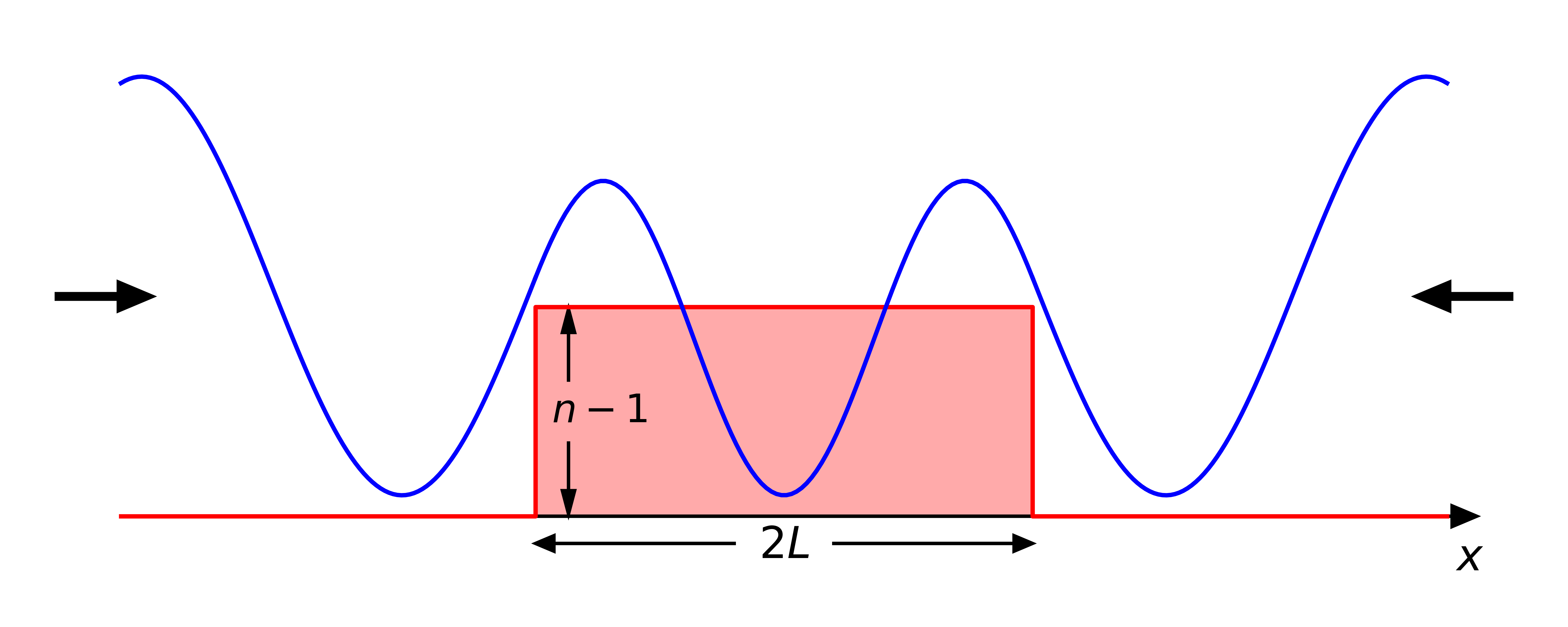
Figure S1: Sketch of the refractive index barrier (red line) of width $2L$ and a constant height of $n-1$. The blue line shows the intensity distribution of the second $Q_{n}$-eigenstate, $\vec{u}^{2}_{n}$, for a wavelength of $\lambda=2\pi$, refractive index $n=1.44$ and a length $L=1.5$. The black arrows indicate that plane waves injected from both sides construct the scattering state.

The corresponding eigenvalues $\theta_{n}^{1,2}$ and eigenstates $\vec{u}_{n}^{1,2}$ then follow as

$$\theta^{1}_{n} =\frac{-4kLn-2\sin(2kLn)}{\left(n^{2}-1\right)\cos(2kLn)-n^{2}-1}, \vec{u}^{1}_{n} =\frac{1}{\sqrt{2}}\left(\begin{array}[]{cc}1\\ 1\end{array}\right),$$ (7)

$$\theta^{2}_{n} =\frac{4kLn-2\sin(2kLn)}{\left(n^{2}-1\right)\cos(2kLn)+n^{2}+1}, \vec{u}^{2}_{n} =\frac{1}{\sqrt{2}}\left(\begin{array}[]{cc}-1\\ 1\end{array}\right).$$ (10)

The integrated intensities of the scattering states inside the barrier read as

$$I_{1} \equiv\int_{-L}^{L}\left|\psi\left(\vec{u}^{1}_{n}\right)\right|^{2}\mathrm{d}x=\frac{-4kLn-2\sin(2kLn)}{kn\left[\left(n^{2}-1\right)\cos(2kLn)-n^{2}-1\right]}=\frac{\theta^{1}_{n}}{kn},$$ (11)

$$I_{2} \equiv\int_{-L}^{L}\left|\psi\left(\vec{u}^{2}_{n}\right)\right|^{2}\mathrm{d}x=\frac{4kLn-2\sin(2kLn)}{kn\left[\left(n^{2}-1\right)\cos(2kLn)+n^{2}+1\right]}=\frac{\theta^{2}_{n}}{kn}.$$ (12)

This result shows that there is a strict linear relation between the stored intensity in the designated scattering region and the eigenvalues of $Q_{n}$ which enables us to tune the intensity inside the scatterer based on the choice of $Q_{n}$-eigenstates (or a superposition of such eigenstates). Taking eigenstates with large eigenvalues results in scattering states that focus into the target region.
To calculate $Q_{\varepsilon}$ we make use of $\mathrm{d}/\mathrm{d}n=\mathrm{d}/\mathrm{d}\varepsilon\cdot\mathrm{d}\varepsilon/\mathrm{d}n=2n\mathrm{d}/\mathrm{d}\varepsilon$, which directly leads to the following expression

$$\frac{I_{1}}{\theta^{1}_{\varepsilon}}=\frac{I_{2}}{\theta^{2}_{\varepsilon}}=\frac{2}{k}.$$ (13)

1.2 $Q_{x}$ for Target Displacement (in 1D)

To construct $Q_{x}$ we take the derivative of the scattering matrix with respect to the position of the barrier. To obtain the eigenvalues associated to the momentum-transfer onto the target we make use of $Q_{x}=k_{\mathrm{in}}-S^{\dagger}k_{\mathrm{out}}S$ [1]. This formula comes from the fact that for only one scatterer (or if we move all scatterers) $Q_{x}$ measures the momentum difference between incoming and outgoing waves. The matrices $k_{\mathrm{in}}$ and $k_{\mathrm{out}}$ read as follows

$$k_{\mathrm{in}}=\left(\begin{array}[]{cc}k&0\\ 0&-k\end{array}\right)=-k_{\mathrm{out}}.$$ (14)

The components of $Q_{x}$ then read

$$-Q_{x,11} =Q_{x,22}=\frac{1}{\Gamma}\left[4k\left(n^{2}-1\right)^{2}\sin^{2}\left(2kLn\right)\right],$$ (15)

$$-Q_{x,12} =Q_{x,21}=\frac{1}{\Gamma}\left[8\mathrm{i}kn\left(n^{2}-1\right)\sin\left(2kLn\right)\right],$$ (16)

with $\Gamma\equiv-\left(n^{2}-1\right)^{2}\cos\left(4kLn\right)+n^{2}\left(n^{2}+6\right)+1>0\enskip\forall n,k,L$. The solution of the eigenproblem associated with $Q_{x}$ is

$$\theta^{1,2}_{x} =\pm\frac{\sqrt{8}k\left(n^{2}-1\right)\sin\left(2kLn\right)}{\sqrt{\Gamma}},$$ (17)

$$\vec{u}^{1,2}_{x} =\mp\frac{1}{N_{1,2}}\left(\frac{-\mathrm{i}}{4n}\left[\sqrt{2\Gamma}\pm 2\left(n^{2}-1\right)\sin\left(2kLn\right)\right],1\right)^{T},$$ (18)

where $N_{1,2}=|\vec{u}^{1,2}_{x}|$ is the norm of the eigenvectors. We then calculate the quantity $F_{1,2}$, which we will show to be proportional to the momentum transfer onto the target:

$$F_{1,2} \equiv\left|\psi\left(\vec{u}^{1,2}_{x},x=-L\right)\right|^{2}-\left|\psi\left(\vec{u}^{1,2}_{x},x=+L\right)\right|^{2}$$

$$=\mp\frac{4\sqrt{2}\sin\left(2kLn\right)}{\sqrt{\Gamma}},$$ (19)

where the first argument in the parentheses tells us which eigenvector of $Q_{x}$ is used in the calculation. We then compare these two quantities with the eigenvalues $\theta_{x}^{1,2}$ of $Q_{x}$ and see that

$$\frac{\theta_{x}^{1}}{F_{1}}=\frac{\theta_{x}^{2}}{F_{2}}=-\frac{k\left(n^{2}-1\right)}{2}.$$ (20)

This result tells us that there is a strict linear relation between the eigenvalues of $Q_{x}$ and the difference in intensities at the left and right boundary of the barrier, $F_{i}$. The eigenvalues $\theta^{1,2}_{x}$ are equal to the momentum difference between incoming and outgoing waves, i.e., $\Delta k=\theta_{x}$ [1]. Conservation of momentum then tells us that a momentum of $\Delta k$ is transferred to the target. We work in the stationary case, thus this momentum transfer onto the target is the same at all times. The average force, $F$, experienced by the target is the momentum transfer per unit time interval and since the momentum transfer is stationary, it is equal to the force. This implies that the quantities $F_{i}$ we have defined above are proportional to the force the target experiences from the scattering of the wave. This enables us to tune the degree of force exerted onto the target and even control the direction of it.

1.3 $Q_{R}$ for Radial Change (in 1D)

The one-dimensional analogue to the radius $R$ of a circle is the length $L$ of a region with raised refractive index. We therefore investigate the behaviour of $Q_{L}=-\mathrm{i}S^{-1}\mathrm{d}S/\mathrm{d}L$, whose elements are given by

$$Q_{L,11} =Q_{L,22}=-\frac{2k\left(n^{2}-1\right)\left[3n^{2}+\left(n^{2}-1\right)\cos(4kLn)+1\right]}{-\left(n^{2}+6\right)n^{2}+\left(n^{2}-1\right)^{2}\cos(4kLn)-1},$$ (21)

$$Q_{L,12} =Q_{L,21}=-\frac{8kn^{2}\left(n^{2}-1\right)\cos(2kLn)}{-\left(n^{2}+6\right)n^{2}+\left(n^{2}-1\right)^{2}\cos(4kLn)-1}.$$ (22)

The solution of the corresponding eigenproblem yields

$$\theta^{1}_{L} =\frac{-4k\left(n^{2}-1\right)\cos^{2}(kLn)}{\left(n^{2}-1\right)\cos(2kLn)-n^{2}-1}, \vec{u}^{1}_{L} =\frac{1}{\sqrt{2}}\left(\begin{array}[]{cc}1\\ 1\end{array}\right),$$ (25)

$$\theta^{2}_{L} =\frac{4k\left(n^{2}-1\right)\sin^{2}(kLn)}{\left(n^{2}-1\right)\cos(2kLn)+n^{2}+1}, \vec{u}^{2}_{L} =\frac{1}{\sqrt{2}}\left(\begin{array}[]{cc}-1\\ 1\end{array}\right).$$ (28)

The intensities at the boundaries of the barrier are

$$P_{1} \equiv 2\left|\psi\left(\vec{u}^{1}_{L},x=\pm L\right)\right|^{2}=\frac{-8\cos^{2}(kLn)}{\left(n^{2}-1\right)\cos(2kLn)-n^{2}-1}=\frac{2\theta_{L}^{1}}{k\left(n^{2}-1\right)},$$ (29)

$$P_{2} \equiv 2\left|\psi\left(\vec{u}^{2}_{L},x=\pm L\right)\right|^{2}=\frac{8\sin^{2}(kLn)}{\left(n^{2}-1\right)\cos(2kLn)+n^{2}+1}=\frac{2\theta_{L}^{2}}{k\left(n^{2}-1\right)},$$ (30)

for each eigenstate of $Q_{L}$. In contrast to $Q_{n}$ whose eigenvalues represent the integrated intensity over the target region, the above result shows that the eigenvalues of $Q_{L}$ correspond to the intensities at the target’s boundary which can be again tuned by choosing a certain $Q_{L}$-eigenstate (or a superposition of such eigenstates).

2 Derivation of Eq. 2

In the following we will sketch the derivation of Eq. 2 from the main text involving the expectation value of the generalised Wigner-Smith (GWS) operator with respect to some arbitrary input vector $\ket{\chi}$. All conventions are taken from [2] (see also [3, 4]). The scattering matrix $S$ for a system described by the Helmholtz equation can be written as

$$S=-\mathbbm{1}+2\mathrm{i}V^{\dagger}GV,\enskip\mathrm{where}\enskip G=\left(\Delta+U(\vec{x})+\mathrm{i}VV^{\dagger}\right)^{-1}\enskip\mathrm{and}\enskip U(\vec{x})=k^{2}\varepsilon(\vec{x}),$$ (31)

where $G$ is the system’s Green’s function, $\Delta$ is the Laplacian, $U$ determines the scattering environment and $V$ describes the coupling to the leads. The derivative of the scattering matrix can then be written as,

$$\frac{\mathrm{d}S}{\mathrm{d}\alpha} =-2\mathrm{i}V^{\dagger}G\frac{\mathrm{d}U}{\mathrm{d}\alpha}GV,$$ (32)

where we have assumed that only the scattering environment $U$ depends on $\alpha$, but not the coupling matrix $V$. Under the further assumption of a unitary $S$-matrix the following useful identity was derived in [2] for the Green’s function $G$,

$$-2\mathrm{i}G^{\dagger}VV^{\dagger}G=G-G^{\dagger}.$$ (33)

With a unitary scattering matrix we can then write $Q_{\alpha}=-\mathrm{i}S^{-1}\frac{\mathrm{d}S}{\mathrm{d}\alpha}$ as,

$$Q_{\alpha} =-2S^{\dagger}V^{\dagger}G\frac{\mathrm{d}U}{\mathrm{d}\alpha}GV$$ (34)

$$=2\left(\mathbbm{1}+2\mathrm{i}V^{\dagger}G^{\dagger}V\right)V^{\dagger}G\frac{\mathrm{d}U}{\mathrm{d}\alpha}GV=2V^{\dagger}\left(G-G+G^{\dagger}\right)\frac{\mathrm{d}U}{\mathrm{d}\alpha}GV$$ (35)

$$Q_{\alpha} =2V^{\dagger}G^{\dagger}\frac{\mathrm{d}U}{\mathrm{d}\alpha}GV.$$ (36)

The wavefunction inside the scattering system for an arbitrary input vector $\ket{\chi}$ can be written as [2],

$$\ket{\psi_{\chi}}=2\mathrm{i}GV\ket{\chi},$$ (37)

resulting in the following expression for the expectation value of $Q_{\alpha}$,

$$\bra{\chi}Q_{\alpha}\ket{\chi}=\frac{1}{2}\bra{\psi_{\chi}}\frac{\mathrm{d}U}{\mathrm{d}\alpha}\ket{\psi_{\chi}}.$$ (38)

This novel result now allows us to extract information about the local wave intensity inside the scattering medium out of the asymptotic information encoded in the scattering matrix $S$.
As a simple test of the above relation, we take the derivative of $U$ with respect to $k$ and we get

$$Q_{k}=4kV^{\dagger}G^{\dagger}\varepsilon GV\equiv Q_{d},$$ (39)

which is exactly the result for the dwell-time operator as given in [2, 4]. Keeping in mind that the dwell time operator and the Wigner-Smith time-delay operator are the same for a vanishing $k$-dependence of $V$ [2, 4], we have thus shown that our new relation is perfectly consistent with this established case.

3 Linear Relations in Two Dimensions

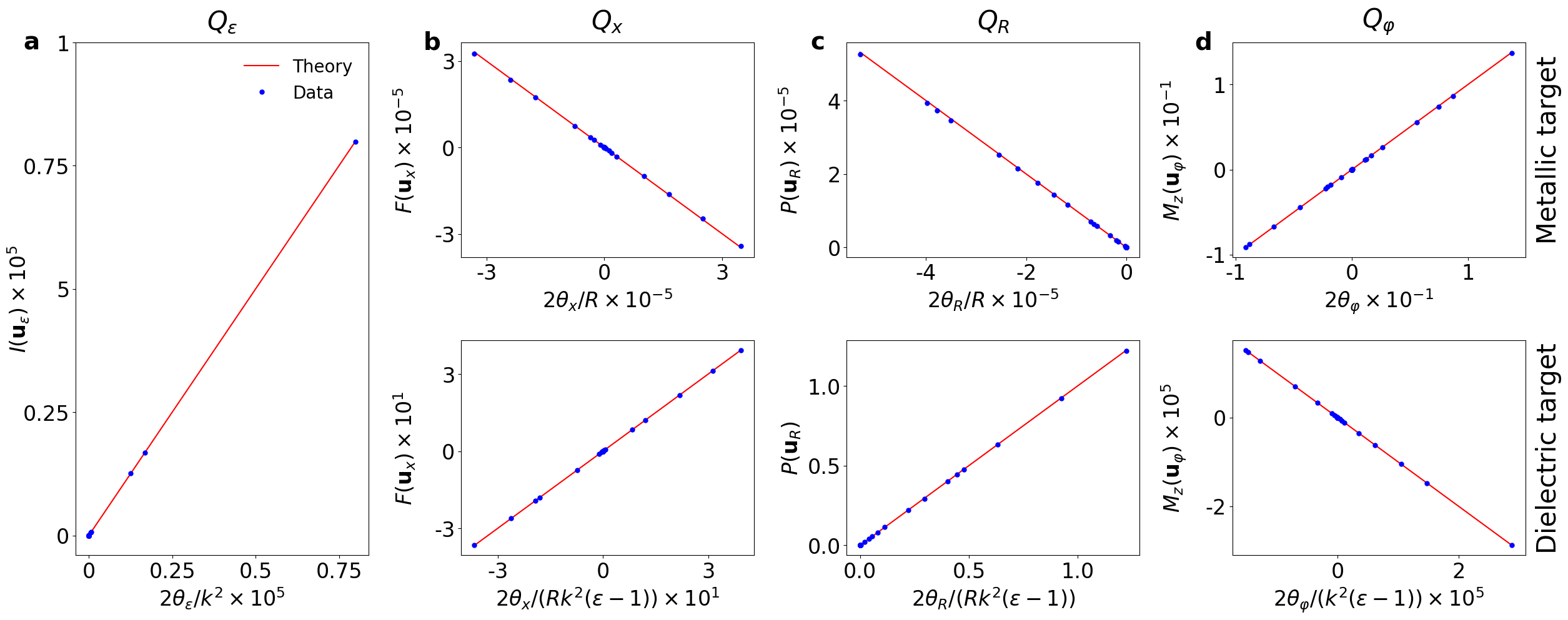
Figure S2: Linear relations of the GWS-eigenvalues with the quantities defined in Eqs. (40)-(53), for $N=20$ propagating modes and a wavelength of $\lambda\approx 0.1W$, where $W$ is the width of the waveguide. The simulation is carried out in the waveguide geometry depicted in Fig. 1 of the main text. The simulated data is depicted by the blue dots and shows an excellent agreement with the theoretical predictions (red line) for all cases (without any free parameters). a, Linear relation between $\theta_{\varepsilon}$ and the stored intensity $I$ for a Teflon ($\varepsilon=2.0736$) target (radius $R=0.0165W$). b, Upper (lower) plot shows the linear relation between $\theta_{x}$ and $F$ for a metallic (Teflon) target ($R=0.0825W$). c, Upper (lower) plot shows the linear relation between $\theta_{R}$ and $P$ for a metallic (Teflon) target. d, Upper (lower) plot shows the linear relation between $\theta_{\varphi}$ and $M_{z}$ for a metallic (Teflon) square target (side length $0.165W$).

Building up on the insights gained in the previous section, we can now prove the linear relations written down in Eqs. (3) and (4) of the main text. We start by proving the relation between $\theta_{\varepsilon}$ and the intensity integrated over the target’s area. Taking the derivative of the scattering environment with respect to the dielectric constant of a single scatterer results in $\mathrm{d}U/\mathrm{d}\varepsilon=k^{2}A_{\mathrm{scat}}\left(\vec{r}\right)$, where $A_{\mathrm{scat}}$ parameterises the area of the scatterer and is equal to one inside the target and zero outside. This then gives

$$I\left(\ket{u_{\varepsilon}^{i}}\right)\equiv\int\lvert\psi\left(\ket{u_{\varepsilon}^{i}}\right)\rvert^{2}\mathrm{d}A=\frac{2\theta_{\varepsilon}^{i}}{k^{2}},$$ (40)

where the integral is performed over the area $A$ of the target scatterer. This equation is numerically confirmed in Fig. S2a and equips us with a tool to control the wave intensity inside a target’s area – ranging from no intensity to the theoretical maximum.
Next, we derive in detail the linear relation between the eigenvalues of $Q_{R}$ and the pressure, $P\left(\ket{u_{R}^{i}}\right)\equiv\int_{0}^{2\pi}\left|\psi\left(\rho=R\right)\right|^{2}\mathrm{d}\varphi$, applied to the target. We start by considering a dielectric target, for which $\mathrm{d}U/\mathrm{d}R=k^{2}(\varepsilon-1)\delta\left(\rho-R\right)$. This leads us to

$$\frac{1}{2}\braket{\psi}{\frac{\mathrm{d}U}{\mathrm{d}R}}{\psi} =\frac{k^{2}\left(\varepsilon-1\right)}{2}\int_{0}^{2\pi}\int_{0}^{\infty}\left|\psi\left(\rho,\varphi\right)\right|^{2}\rho\,\delta\left(\rho-R\right)\mathrm{d}\rho\mathrm{d}\varphi$$ (41)

$$=\frac{k^{2}\left(\varepsilon-1\right)R}{2}\int_{0}^{2\pi}\left|\psi\left(\rho=R,\varphi\right)\right|^{2}\mathrm{d}\varphi$$ (42)

$$=\frac{k^{2}\left(\varepsilon-1\right)R}{2}P\left(\ket{u_{R}^{i}}\right).$$ (43)

This derivation provides us with the final result that the pressure is in a linear relation to the eigenvalues of $Q_{R}$

$$P\left(\ket{u_{R}^{i}}\right)\equiv\int_{0}^{2\pi}\left|\psi\left(\rho=R\right)\right|^{2}\mathrm{d}\varphi=\frac{2\theta_{R}^{i}}{Rk^{2}(\varepsilon-1)}.$$ (44)

We confirm this equation numerically in Fig. S2c. To prove a linear relation between the eigenvalues of $Q_{R}$ and the transferred pressure in the case of a metallic target with perfect conductance we first consider the simple example of an infinitely long metallic rod of circular cross-section in vacuum. Effectively this configuration can be reduced to a two-dimensional problem. Due to the simplicity of the geometry, different incoming cylindrical wave modes do not mix, therefore the scattering matrix $S$, which in this case is just a unitary diagonal reflection matrix $r$, reads

$$\left[r\right]_{nn}=-\frac{\mathrm{H}_{n}^{(2)}\left(kR\right)}{\mathrm{H}_{n}^{(1)}\left(kR\right)},$$ (45)

where $\mathrm{H}_{n}^{(1)}$ and $\mathrm{H}_{n}^{(2)}$ are the Hankel functions of the first and second kind, respectively. The knowledge of the reflection matrix then allows us to compute the GWS-operator $Q_{R}$, whose elements on the diagonal read

$$\left[Q_{R}\right]_{nn}=-\frac{4}{\pi R\left[\mathrm{J}_{n}\left(kR\right)^{2}+\mathrm{Y}_{n}\left(kR\right)^{2}\right]},$$ (46)

where $J_{n}$ and $Y_{n}$ are the Bessel functions of the first and second kind, respectively. The wavefunction around the metallic rod comprised of the incident and scattered wave is

$$\psi\left(\rho,\varphi\right)=\frac{1}{2}\sum_{n=-\infty}^{\infty}b_{n}e^{\mathrm{i}n\varphi}\left[\mathrm{H}_{n}^{(2)}\left(k\rho\right)+\left[r\right]_{nn}\mathrm{H}_{n}^{(1)}\left(k\rho\right)\right],$$ (47)

where $b_{n}$ are the components of the input vector. This leads to the following expression in the case when $b_{n}=1$ for only one $n$ and zero for all other

$$P\equiv\int_{0}^{2\pi}\left|\partial_{\rho}\psi\left(\rho=R\right)\right|^{2}\mathrm{d}\varphi=\frac{8}{\pi R^{2}\left[\mathrm{J}_{n}\left(kR\right)^{2}+\mathrm{Y}_{n}\left(kR\right)^{2}\right]}.$$ (48)

We thus find

$$P\left(\ket{u_{R}^{i}}\right)=-\frac{2\theta_{R}^{i}}{R},$$ (49)

which we confirm numerically in Fig. S2c for a circular metallic target inside a waveguide featuring the same disorder as in Fig. 1 of the main manuscript. The reason why our derivation of the proportionality constant also works for an arbitrary environment as wells as an arbitrary cross-section, is that the proof of the GWS-operator tells us that its eigenvalues $\theta_{\alpha}$ are in a linear relation with the local wave intensity around the target, irrespectively of the surrounding scattering environment and whether these are waveguide walls or a disordered medium.
Next we consider the eigenvalues of $Q_{x}$, the GWS-operator we get when the parameter $\alpha$ considered is the longitudinal position $x$ of a target. This problem was originally considered in [1], although a proof was only given for the case of longitudinally moving the entire scattering system. Here we close this gap and prove a linear relation between the eigenvalues and the momentum transferred also for a single target inside a disordered medium, using the same strategy as in the preceding paragraph. For a dielectric circular target with radius $R$, the result reads

$$F\left(\ket{u^{i}_{\hat{\vec{n}}}}\right)\equiv\hat{\vec{n}}\cdot\int_{0}^{2\pi}\left(\begin{array}[]{cc}\cos\varphi\\ \sin\varphi\end{array}\right)\left|\psi\left(\rho=R\right)\right|^{2}\mathrm{d}\varphi=\frac{2\theta^{i}_{\hat{\vec{n}}}}{Rk^{2}(\varepsilon-1)},$$ (50)

where the direction of the shift and the corresponding momentum transfer is generalised to an arbitrary direction, which is parametrised by the unit vector $\hat{\vec{n}}$ and the integral is performed along the boundary of the circular target (a generalization to arbitrary target shapes is also possible). In the presence of a metallic target the result is

$$F\left(\ket{u_{\hat{\vec{n}}}^{i}}\right)\equiv\hat{\vec{n}}\cdot\int_{0}^{2\pi}\left(\begin{array}[]{cc}\cos\varphi\\ \sin\varphi\end{array}\right)\left|\partial_{\rho}\psi\left(\rho=R\right)\right|^{2}\mathrm{d}\varphi=-\frac{2\theta_{\hat{\vec{n}}}^{i}}{R}.$$ (51)

Numerical results confirming these relations for $\hat{\vec{n}}=(1,0)^{T}$ can be found in Fig. S2b.
The same approach also works when considering the eigenvalues of $Q_{\varphi}$ that are in a linear relation with the torque transferred to the target. In the case of a dielectric target this relation reads

$$M_{z}\left(\ket{u_{\varphi}^{i}}\right)\equiv\int_{\mathcal{C}}\left[\vec{m}_{\perp}\left(\vec{c}\right)\times\vec{n}\left(\vec{c}\right)\left|\psi\left(\vec{c}\right)\right|^{2}\right]_{z}\mathrm{d}s=-\frac{2\theta^{i}_{\varphi}}{k^{2}(\varepsilon-1)},$$ (52)

where the integral is taken along the target’s boundary described by the curve $\mathcal{C}$ and parametrised by $\vec{c}$. The expression $\vec{n}\left(\vec{c}\right)\left|\psi\left(\vec{c}\right)\right|^{2}$ denotes the normal force at every point of the boundary excised by the electric field and $\vec{m}_{\perp}\left(\vec{c}\right)$ is the part of the distance from the boundary to the target’s center of mass that is normal to $\vec{n}$, i.e., the lever. We find that in the presence of a metallic target, the eigenvalues $Q_{\varphi}$ are proportional to

$$M_{z}\left(\ket{u_{\varphi}^{i}}\right)\equiv\int_{\mathcal{C}}\left[\vec{m}_{\perp}\left(\vec{c}\right)\times\vec{n}\left(\vec{c}\right)\left|\partial_{\vec{n}}\psi\left(\vec{c}\right)\right|^{2}\right]_{z}\mathrm{d}s=2\theta^{i}_{\varphi},$$ (53)

where $\vec{n}\left(\vec{c}\right)\left|\partial_{\vec{n}}\psi\left(\vec{c}\right)\right|^{2}$ denotes the normal force at every point of the boundary excised by the electric field. These two equations are numerically verified in Fig. S2d for the case of a square target.

4 Applying Pressure with the GWS-Operator

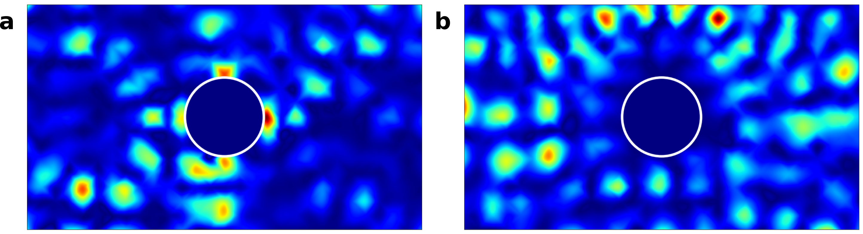
Figure S3: a, Measured spatial intensity distribution for the scattering state created by the eigenvector $\ket{u_{R}^{\mathrm{max}}}$ of $Q_{R}$ corresponding to the largest eigenvalue $|\theta_{R}^{\mathrm{max}}|\approx 709$. A strong focus on the metallic target’s boundary (radius $R=14$ mm) can clearly be observed in the experimental data, verifying our prediction that these states control the applied pressure. b, To contrast this we show here the experimentally obtained intensity distribution for a state corresponding to a small eigenvalue $|\theta_{R}^{\mathrm{small}}|\approx 86$.

In this section we look at the GWS-operator $Q_{R}=-\mathrm{i}S^{-1}\mathrm{d}S/\mathrm{d}R$, where $R$ is the radius of a metallic circular scatterer (our approach also works for more complicated target shapes). For the corresponding eigenvectors $\ket{u_{R}^{i}}$ we analytically showed in the preceding section that there exists a linear relation between the radiation pressure applied to such a metallic target and the corresponding eigenvalue $\theta_{R}^{i}$ of the following form:

$$P\left(\ket{u_{R}^{i}}\right)\equiv\int_{0}^{2\pi}\left|\partial_{\rho}\psi\left(\rho=R\right)\right|^{2}\mathrm{d}\varphi=-2\theta_{R}^{i}/R,$$ (54)

where the integral is along the boundary of the circular scatterer with radius $R$ and $\psi$ is the electric field distribution of the corresponding eigenstate $\ket{u_{R}^{i}}$. In other words, the eigenstates $\ket{u_{R}^{i}}$ of $Q_{R}$ are characterised by a well-defined radiation pressure $P$ that they apply to the dielectric target scatterer. The pressure applied to a chosen target can thus be maximised by injecting eigenstates $\ket{u_{R}^{\mathrm{max}}}$ corresponding to the largest eigenvalues $\theta_{R}^{\mathrm{max}}$. The experimentally measured scattering state of the eigenstate associated to the largest eigenvalue can be seen in Fig. S3a, where the experiment was carried out in a waveguide featuring a disorder (see Fig. 1). We can clearly see that the state has a strong intensity build-up on all sides of the boundary of the chosen scatterer. Constructing $Q_{R}$ with a dielectric scatterer (rather than a metallic one) as a target yields the following linear relation between the radiation pressure $P$ and the eigenvalues $\theta_{R}^{i}$,

$$P\left(\ket{u_{R}^{i}}\right)\equiv\int_{0}^{2\pi}\left|\psi\left(\rho=R\right)\right|^{2}\mathrm{d}\varphi=\frac{2\theta_{R}^{i}}{Rk^{2}\left(\varepsilon-1\right)}.$$ (55)

5 Comparing the GWS-Method and the Field Matrix Method

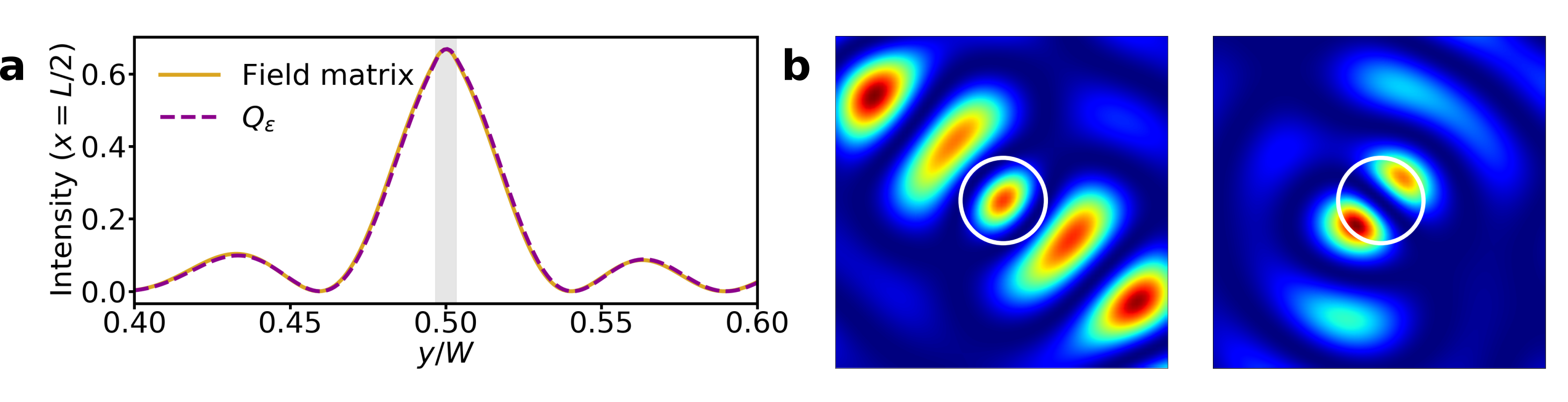
Figure S4: a, Simulated intensity of the state calculated with the field matrix method [5], which produces an optimal focus in a single point, and the highest $Q_{\varepsilon}$-eigenstate at the center of the target ($x=L/2$) as a function of the transverse coordinate $y$ (the grey-shaded region marks the extension of the target scatterer). In these simulations we use the same geometry as in the experiment, featuring a disorder, but with a frequency of 30 GHz resulting in 20 propagating modes and a wavelength of 1 cm. The diameter of the target is 0.69 mm which corresponds to 10% of the wavelength inside the target. The resulting state is identical to the highest $Q_{\varepsilon}$-eigenstate, confirming our prediction that we are able to achieve optimal focus. b, Comparison of the field matrix result (left) with a focus point in the middle of the target to the highest $Q_{\varepsilon}$-eigenstate (right) when $\varepsilon$ is varied inside the entire target with radius 10.4 mm. The two peaks produced by the GWS-method results in a two-fold increase of the integrated intensity in the target as compared to the one peak produced by the field matrix method.

Here we verify explicitly that our micro-manipulation protocol is indeed optimal by comparing it to a procedure proposed in [5]. There the authors achieve a focus onto a point inside a scattering medium by utilizing the field matrix $e(x)$, which relates the field at a depth $x$ inside the scattering medium to the incident field in the waveguide’s leads. The components of the field matrix $e_{ab}(x)$ connect the field in channel $b$ at depth $x$ with the field in channel $a$ at the waveguide’s leads, i.e., $E_{b}(x)=e_{ba}(x)E_{a}$, where $E_{a}$ and $E_{b}(x)$ are the fields in channels $a$ and $b$. Optimal focus, i.e., maximizing $\lvert E_{\beta}(x)\rvert$, at a target point $\beta$ can now be achieved by shaping the incident wavefront as

$$E_{a}^{\mathrm{opt}}=e^{*}_{\beta a}(x)I_{\beta}^{-1/2}(x),$$ (56)

with $I_{\beta}(x)=\sum_{a}\lvert e_{\beta a}(x)\rvert^{2}$ (for a proof see [6]). In Fig. S4a we compare the focus achieved by the field matrix method with the one achieved with the highest $Q_{\varepsilon}$-eigenstate for a circular target scatterer with a very small diameter $D$ (a very small target allows us to converge to the limit of focusing on a point, as considered in the field-matrix method). Our comparison, indeed, shows that the highest $Q_{\varepsilon}$-eigenstate is indistinguishable from the one constructed by the field matrix method, i.e., they both deliver the optimal focus in form of a single peak in the center of the scatterer. In contrast to the field matrix method which, however, can only focus onto a single point, the GWS-concept also enables optimal focusing into an extended area of arbitrary size. Focusing into an extended area requires more than one peak such that the field matrix method would then already have to know where exactly all these peaks have to lie, which is equivalent to already knowing the state that leads to optimal focus in the first place. To demonstrate that the GWS-concept is able to focus in an extended area we show in Fig. S4b the spatial intensity distribution of the highest $Q_{\varepsilon}$-eigenstate around a target scatterer with a larger area. In order to maximise the stored intensity, $Q_{\varepsilon}$ constructs the highest eigenstate such that two peaks fit inside the scatterer, resulting in a two-fold increase of the stored intensity as compared to the field-matrix solution with just one peak in the center of the target.

6 Incomplete Access to Scattering Channels

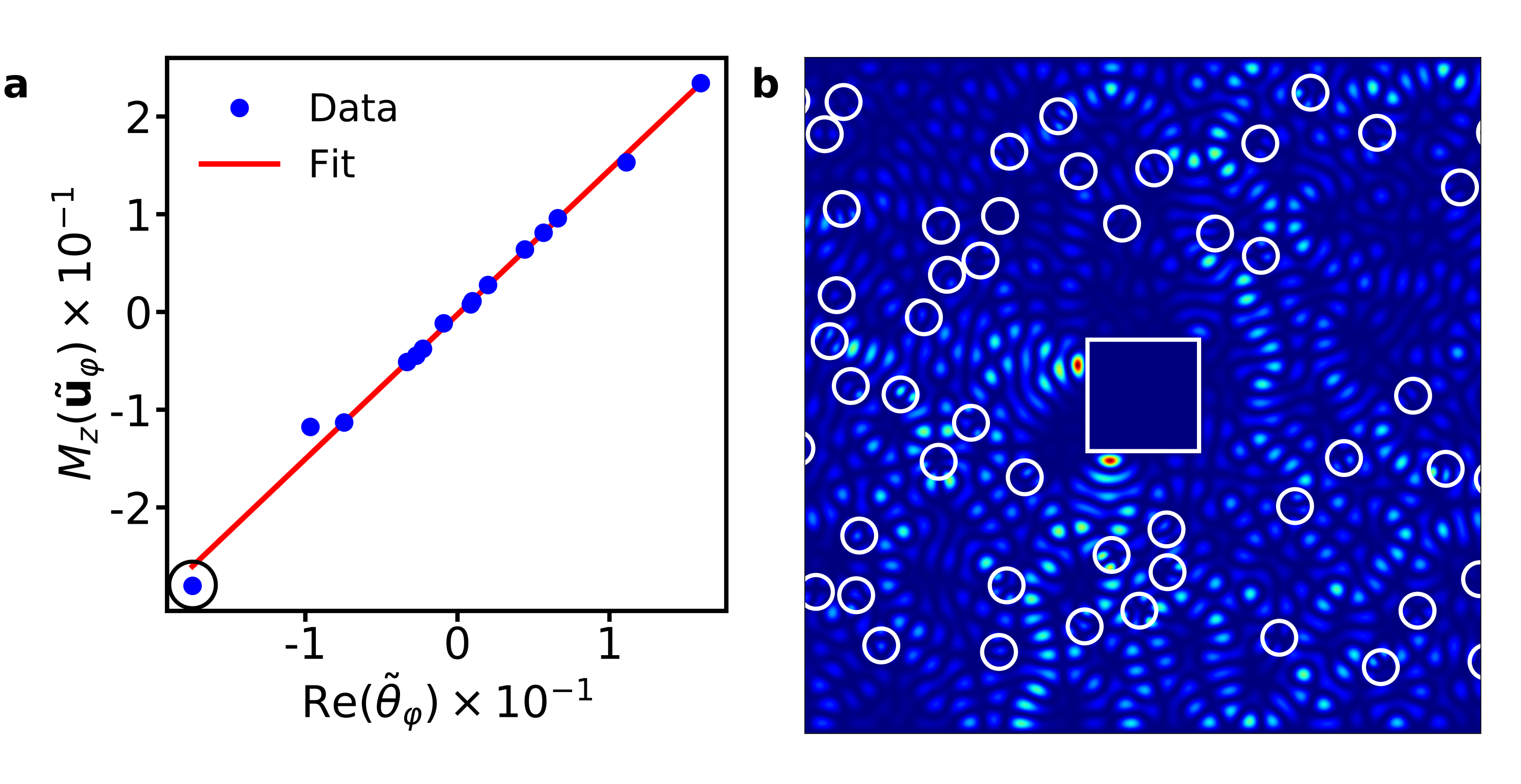
Figure S5: a, Linear relation between the torque $M_{z}\left(\ket{\tilde{u}_{\varphi}}\right)$ and the real part of $\tilde{q}_{\varphi}$ - eigenvalues $\mathrm{Re}\left(\tilde{\theta}_{\varphi}\right)$ in the case of incomplete access to scattering channels. The target here is a metallic square embedded into a disorder of 300 randomly distributed Teflon scatterers, where the whole system has a reflectivity of $R\approx 0.87$. Despite the limitations an approximately linear behaviour can be clearly seen. Here, $N=40$ propagating modes were used, where the $M=10$ highest ones are neglected in the calculation of $\tilde{q}_{\varphi}$ to simulate a low numerical aperture. In the SVD-procedure, we project onto the 15 highest reflecting states, which results in a correlation coefficient of $r=0.997$. The black circle marks the eigenvalue with the largest absolute value of $\mathrm{Re}\left(\tilde{\theta}_{\varphi}\right)$ whose corresponding eigenstate is shown in b. b, Spatial intensity distribution of the $\tilde{q}_{\varphi}$-eigenstate corresponding to the largest absolute value of $\mathrm{Re}\left(\tilde{\theta}_{\varphi}\right)$ which focuses onto the edges of the square target in order to maximise the transferred torque.

In the main document we explore different realisations of GWS-operators for the ideal case where we have access to the full scattering matrix, $S$. Since it is experimentally challenging to measure the entire scattering matrix, we numerically show that our approach also works in the regime of a sub-unitary $S$-matrix. For this case we consider the same waveguide ($L=6W$) as in the main document but fill it with $300$ randomly distributed Teflon scatterers ($R=0.025W$, $n=1.44$) and a square metallic target (side length $0.165W$) at $x$-position $L/6$. Instead of the full scattering matrix, we now take only the reflection matrix $r$ for the calculation of the GWS-operator, since in the experiment both transmission and reflection measurements are not always possible. Experiments also suffer from a low numerical aperture (LNA), which we take into account in our simulation by removing the $M$ highest modes from $r$ such that we are left with a $(N-M)\times(N-M)$ matrix $r_{\mathrm{LNA}}$, where $N$ is the number of modes. When we use only the reflection matrix to construct an operator $q_{\varphi}=-\mathrm{i}r^{-1}\mathrm{d}r/\mathrm{d}\varphi$ its eigenvalues turn out to be $\theta_{\varphi}^{i}=\left(M_{z}(\vec{u}_{\varphi}^{i})+\mathrm{i}\vec{u}_{\varphi}^{i,\dagger}t^{\dagger}\mathrm{d}t/\mathrm{d}\varphi\vec{u}_{\varphi}^{i}\right)/(2\langle r^{\dagger}r\rangle)$ [1], where $\langle r^{\dagger}r\rangle$ is the global reflectance of the eigenstate and the loss of information manifests itself in complex eigenvalues caused by the second term containing the transmission matrix $t$. From this expression we may thus conclude that our procedure based on the reflection matrix only will work better for higher total reflection and for the case that the target is placed at the beginning of the waveguide (placing it on the end would result in far less intensity reaching it). In order to still maintain a correlation between the eigenvalues of $q_{\varphi}$ and the total torque acting on the target scatterer, we also have to restrict ourselves to channels that are strongly reflecting to minimise the term with the transmission matrix $t$. We achieve this by using a singular-value decomposition of $r_{\mathrm{LNA}}=U\Sigma V^{\dagger}$, where the matrices $U$ and $V$ contain the column wise the left and right singular vectors (not to be confused with the scattering environment and the coupling matrix, respectively) and the matrix $\Sigma=\mathrm{diag}\left(\left\{\sigma_{n}\right\}\right)$ contains the singular values on its diagonal. In order to project on the highly reflecting channels we pick a certain subset of large singular values $\tilde{\Sigma}=\mathrm{diag}\left(\left\{\tilde{\sigma}_{n}\right\}\right)$ as well as the associated left and right singular vectors $\tilde{U}$ and $\tilde{V}$. Equipped with these matrices we can construct an effective inverse $r_{\mathrm{LNA}}^{-1}=\tilde{V}\left(\tilde{U}^{\dagger}r_{\mathrm{LNA}}\tilde{V}\right)^{-1}\tilde{U}^{\dagger}$ and also project the derivative of $r_{\mathrm{LNA}}$ onto this subspace with the proper projection operators $P_{\tilde{U}}=\tilde{U}\tilde{U}^{\dagger}$ and $P_{\tilde{V}}=\tilde{V}\tilde{V}^{\dagger}$ [1]. As a final result we obtain:

$$\tilde{q}_{\varphi}=-\mathrm{i}\tilde{V}(\tilde{U}^{\dagger}r_{\mathrm{LNA}}\tilde{V})^{-1}\tilde{U}^{\dagger}\tilde{U}\tilde{U}^{\dagger}\frac{\mathrm{d}r_{\mathrm{LNA}}}{\mathrm{d}\varphi}\tilde{V}\tilde{V}^{\dagger}.$$ (57)

In Fig. S5a one can see that Eq. (53) is almost perfectly fulfilled, i.e., our protocol works even for the case where only parts of the scattering matrix are available. This, however, comes with the caveat that the system needs to be highly reflecting (transmitting) when we work only with the reflection (transmission) matrix. Fig. S5b shows the spatial intensity distribution of the $\tilde{q}_{\varphi}$-eigenstate which transfers the maximal amount of torque.

References

- [1] P. Ambichl, A. Brandstötter, J. Böhm, M. Kühmayer, U. Kuhl, and S. Rotter, “Focusing inside Disordered Media with the Generalized Wigner-Smith Operator,” Physical Review Letters, vol. 119, July 2017.
- [2] P. Ambichl, Coherent Wave Transport: Time Delay and Beyond. PhD thesis, TU Wien, 2016.
- [3] Y. V. Fyodorov and H.-J. Sommers, “Statistics of resonance poles, phase shifts and time delays in quantum chaotic scattering: Random matrix approach for systems with broken time-reversal invariance,” Journal of Mathematical Physics, vol. 38, pp. 1918–1981, Apr. 1997.
- [4] S. Rotter and S. Gigan, “Light fields in complex media: Mesoscopic scattering meets wave control,” Reviews of Modern Physics, vol. 89, Mar. 2017.
- [5] X. Cheng and A. Z. Genack, “Focusing and energy deposition inside random media,” Opt. Lett., vol. 39, pp. 6324–6327, Nov 2014.
- [6] I. M. Vellekoop and A. P. Mosk, “Universal optimal transmission of light through disordered materials,” Phys. Rev. Lett., vol. 101, p. 120601, Sep 2008.