On Critical Point for Functions with Bounded Parameters

Abstract

Selection of descent direction at a point plays an important role in numerical optimization for minimizing a real valued function. In this article, a descent sequence is generated for the functions with bounded parameters to obtain a critical point. First, sufficient condition for the existence of descent direction is studied for this function and then a set of descent directions at a point is determined using linear expansion. Using these results a descent sequence of intervals is generated and critical point is characterized. This theoretical development is justified with numerical example.

keywords Line search technique, Markov difference, Interval ordering, Descent direction, Critical point.

1 Introduction

In most of the mathematical models, the parameters vary in some bounds which can be estimated from historical data. These uncertain parameters can be considered as intervals. In that case, the functions involved in the model here known as functions with bounded parameters as intervals. Interval analysis plays an important role to handle these functions. This article has studied some properties of these type functions, $\breve{F}$ from $\mathbf{R}^{n}$ to the set of closed intervals, whose parameters are intervals. An example of such type function is
$\breve{F}(x,y)=e^{[-3,3]x^{3}}\oplus[4,5]xy^{5}$. In the literature of interval analysis, Markov is the pioneer who has studied different areas of modern mathematics using interval analysis ( see [5], [6], [10], [11], [12], [13] etc. ). Markov has introduced nonstandard substraction between two closed intervals( known as Markov difference, $\ominus_{M}$), which has explored calculus of functions with bounded parameters and its application in several areas in recent times (see [1], [2], [9], [15], [16] etc.). Another nonstandard difference, known as gH-difference, in the set of intervals is introduced in [18] and further developed in [4], [7],[17] etc. . It is justified in [3] that gH difference coincides with Markov difference in case of compact intervals. Markov difference is more comfortable for use in numerical computations. Hence in this article we have accepted Markov difference and proceed to develop an iterative process for generating a descent sequence of intervals. This concept may be extended further to develop a descent sequence of points which may converge to a local minimum point of a function with interval parameters under reasonable conditions. This can explore a new area of numerical optimization, which may be considered as the possible scope of the present contribution. At this present stage we focus on characterizing descent direction, generating descent sequence of intervals for a function with interval parameters, which provides the critical point of the function.

Some prerequisites on interval analysis are discussed in Section 2. In Section 3, Markov difference is used to derive the linear expansion of $\breve{F}$ and existence of descent direction of $\breve{F}$ at a point $x$ is studied. Section 4 is devoted for generating descent sequence of intervals which determines the critical point of $\breve{F}$. Section 5 provides concluding remarks with future scope.

2 Prerequisites

$K(\textbf{R})$ denotes the set of all compact intervals on R throughout this article . $\breve{\alpha}\in K(\mathbf{R})$ is the closed interval of the form $[\underline{\alpha},\overline{\alpha}]$ where $\underline{\alpha}\leq\overline{\alpha}$. For two points $\alpha_{1}$ and $\alpha_{2}$,(not necessarily $\alpha_{1}\leq\alpha_{2}$), $\breve{\alpha}$ can be written as $\breve{\alpha}=[\alpha_{1}\vee\alpha_{2}]$. A real number $r$ can be represented as a degenerate interval denoted by $\breve{r}$ as $\breve{r}=[r,r]$ or $r.\breve{I}$, where $\breve{I}=[1,1]$. The null interval is $\breve{0}=[0,0]=0$.
In $K(\mathbf{R})$, the norm $(\|.\|)$ of an interval $\breve{\alpha}$ is defined as $\|\breve{\alpha}\|=\max\left\{|\underline{\alpha}|,|\overline{\alpha}|\right\}$ ([8] ) which is associated with the metric $d(\breve{\alpha},0)=\|\breve{\alpha}\|$ and $d(\breve{\alpha},\breve{\beta})=\max\left\{|\underline{\alpha}-\underline{\beta}|,\leavevmode\nobreak\ |\overline{\alpha}-\overline{\beta}|\right\}$.
$K(\mathbf{R})$ is not a complete ordered set. Following interval ordering is used throughout the article..
For $\breve{\alpha}$, $\breve{\beta}\in K(\mathbf{R})$, $\breve{\alpha}\preceq\breve{\beta}\Leftrightarrow\underline{\alpha}\leq\underline{\beta}$, $\overline{\alpha}\leq\overline{\beta}$ and $\breve{\alpha}\neq\breve{\beta}$; $\breve{\alpha}\prec\breve{\beta}\Leftrightarrow\underline{\alpha}<\underline{\beta}$ and $\overline{\alpha}<\overline{\beta}$.

The other interval order relations $`\succeq^{\prime}$ and ${}^{\prime}\succ^{\prime}$ can be defined in a similar way.

Additive inverse in $\left\langle K(\mathbf{R}),\oplus,\odot\right\rangle$ may not exist, that is, $\breve{\alpha}\ominus\breve{\alpha}$ is not necessarily $\breve{0}$ according to this approach. The non-standard subtraction due to [9], denoted by $\ominus_{M}$, provides additive inverse, which is

$$\breve{\alpha}\ominus_{M}\breve{\beta}=\left[\min\left\{\underline{\alpha}-\underline{\beta},\overline{\alpha}-\overline{\beta}\right\},\max\left\{\underline{\alpha}-\underline{\beta},\overline{\alpha}-\overline{\beta}\right\}\right]$$ (1)

Following properties of $\ominus_{M}$ due to [5] and [9] are used throughout the article.
(i) $\breve{\alpha}\ominus_{M}\breve{\alpha}=\breve{0}$ ; (ii) $\ominus_{M}\breve{\alpha}=(-1)\breve{\alpha}=[-\overline{\alpha},-\underline{\alpha}]$

Limit and continuity of $\breve{F}$ are understood in the sense of $\parallel.\parallel$ due to [9]. Following results due to [9] are summarized for $\breve{F}:\mathbf{R}\rightarrow K(\mathbf{R})$, $\breve{F}(x)=[\underline{F}(x),\overline{F}(x)]$, where $\underline{F},\overline{F}:\mathbf{R}\rightarrow\mathbf{R}$, $\underline{F}(x)\leq\overline{F}(x)$ $\forall\leavevmode\nobreak\ \leavevmode\nobreak\ x\in\mathbf{R}$.

Definition 1 (Definition 2, [9]).

$\breve{F}:\mathbf{R}\rightarrow K(\mathbf{R})$ is differentiable at $x_{0}$ if $\displaystyle\lim_{h\rightarrow 0}\frac{\breve{F}(x_{0}+h)\ominus_{M}\breve{F}(x_{0})}{h}$ exists. The limiting value is the derivative of $\breve{F}$ at $x_{0}$, denoted by $\breve{F}^{\prime}(x_{0})$.
Alternatively if $\exists\breve{F}^{\prime}(x_{0})\in K(\mathbf{R})$ and an error function
$\breve{E}_{x_{0}}:\mathbf{R}\rightarrow K(\mathbf{R})$ at $x$ such that

$$\breve{F}(x_{0}+h)\ominus_{M}\breve{F}(x_{0})=h\odot\breve{F}^{\prime}(x_{0})\oplus\breve{E}_{x_{0}}(h)$$ (2)

$$\text{ where }\lim_{h\rightarrow 0}\breve{E}_{x_{0}}(h)=\breve{0}$$

Theorem 2.1 (Theorem 9, [9]).

If $\breve{F}:\mathbf{R}\rightarrow I(\mathbf{R})$ is
continuous in $\Delta$, where $\Delta=\left[p,q\right]$ and differentiable in $(p,q)$,then $\breve{F}(q)\ominus_{M}\breve{F}(p)\subset\breve{F}^{\prime}(\Delta)(q-p)$, where
$\displaystyle\breve{F}^{\prime}(\Delta)=\cup_{\xi\in\Delta}\breve{F}^{\prime}(\xi)$.

Above results discuss the calculus of interval function on $\mathbf{R}$. In next section some of these results are extended to develop calculus of interval functions on $\mathbf{R}^{n}$.

3 Descent direction for interval function over $\mathbf{R}^{n}$

Definition 2.

For $\breve{F}:\mathbf{R}^{n}\rightarrow K(\mathbf{R})$, the partial derivative
of $\breve{F}$ with respect to $x_{i}$ at ‘$x$ ’ exists if $\underset{h_{i}\rightarrow 0}{\lim}\dfrac{\breve{F}(x_{1},\cdots,x_{i-1},x_{i}+h_{i},x_{i+1},\cdots x_{n})\ominus_{M}\breve{F}(x)}{h_{i}}$ exists. The limiting value is denoted by $\frac{\partial\breve{F}(x)}{\partial x_{i}}$.

In the light of concept of differentiability in (2) of Definition 1, the following can be stated as follows.

Definition 3.

$\breve{F}:\mathbf{R}^{n}\rightarrow K(\mathbf{R})$ is called differentiable at $x_{0}$ if $\frac{\partial\breve{F}(x_{0})}{\partial x_{i}}$ exists $\forall\leavevmode\nobreak\ i$ and an interval function
$\breve{E}_{x_{0}}(h):\mathbf{R}^{n}\rightarrow K(\mathbf{R})$ such that

$$\breve{F}(x_{0}+h)\ominus_{M}\breve{F}(x_{0})=\sum\limits_{i=1}^{n}\left(\oplus h_{i}\odot\frac{\partial\breve{F}(x_{0})}{\partial x_{i}}\right)\oplus\|h\|\odot\breve{E}_{x_{0}}(h)$$

for $\|h\|<\delta$ for some $\delta>0$, where $\lim_{\|h\|\rightarrow 0}\breve{E}_{x_{0}}(h)=\breve{0}$.

Gradient of $\breve{F}$ at $x$ is $(\frac{\partial\breve{F}(x)}{\partial x_{1}},\frac{\partial\breve{F}(x)}{\partial x_{2}},\cdots,\frac{\partial\breve{F}(x)}{\partial x_{n}})^{\prime}$ and denoted by $\nabla\breve{F}(x)$.

Following result is about linear expansion of $\breve{F}$ in inclusion form which will be used further to derive descent direction.

Theorem 3.1.

Let $\Omega$ be an open convex subset of $\mathbf{R}^{n}$ and $\breve{F}:\Omega\rightarrow K(\mathbf{R})$ be differentiable on $\Omega$. Then for any $u,\leavevmode\nobreak\ v\in\Omega$,

$$\breve{F}(v)\ominus_{M}\breve{F}(u)\subset\underset{c\in L.S\{u,v\}}{\cup}\sum_{i=1}^{n}(v_{i}-u_{i})\odot\frac{\partial\breve{F}(c)}{\partial\gamma_{i}}$$ (3)

where $\gamma(t)=u+t(v-u)$, $t\in[0,1]$ and $L.S\{u,v\}$ denotes the line segment joining $u$ and $v$.

Proof.

Since $\Omega$ is convex subset of $\mathbf{R}^{n}$, for $u,v\in\Omega$, $u+t(v-u)$ with $t\in[0,1]$ must belongs to $\Omega$.
Let $\breve{\phi}:[0,1]\rightarrow K(\mathbf{R})$ is defined by
$\breve{\phi}(t)=\breve{F}(\gamma_{1}(t),\gamma_{2}(t),\cdots\gamma_{n}(t))$. Since $\breve{F}(\gamma)$ and $\gamma(t)$ are differentiable, using Definition 3 and first order Taylor expansion of $\gamma$ it can be shown that their composite function $\breve{\phi}$ is differentiable and
$\breve{\phi}^{\prime}(t)=\displaystyle\sum_{i=1}^{n}\gamma_{i}^{\prime}(t)\odot\frac{\partial\breve{F}(\gamma(t))}{\partial\gamma_{i}}=\displaystyle\sum_{i=1}^{n}(v_{i}-u_{i})\odot\frac{\partial\breve{F}(\gamma(t))}{\partial\gamma_{i}}$.

From Theorem 2.1, $\breve{\phi}(1)\ominus_{M}\breve{\phi}(0)\subset\underset{\theta\in[0,1]}{\cup}\breve{\phi}^{\prime}(\theta)$. Here $\breve{\phi}(1)=\breve{F}(v)$ and $\breve{\phi}(0)=\breve{F}(u)$. Hence (3) follows, where $c=a+\theta(b-a)$ for some $\theta$ and $\breve{\phi}^{\prime}(\theta)=\displaystyle\sum_{i=1}^{n}(v_{i}-u_{i})\odot\frac{\partial\breve{F}(c)}{\partial\gamma_{i}}$. ∎

Proposition 1.

Let $\breve{\alpha},\breve{\beta}\in K(\mathbf{R})$. Then $\breve{\alpha}\prec\breve{\beta}$ holds if and only if $\breve{\alpha}\ominus_{M}\breve{\beta}\prec\breve{0}$.

Proof of this result is straight forward from the definition of $\ominus_{M}$.

Definition 4.

$d\in\mathbf{R}^{n}$ is called a descent direction of $\breve{F}$ at $x$ if $\exists$ some $\delta>0$ so that $\breve{F}(x+\alpha d)\prec\breve{F}(x)\leavevmode\nobreak\ \leavevmode\nobreak\ \forall\alpha\in(0,\delta)$.

Notation 1.

Denote $\nabla\breve{F}(x)$ by $\breve{g}(x)$ where
$\breve{g}(x)=\begin{pmatrix}\breve{g}_{1}(x)&\breve{g}_{2}(x)&\cdots&\breve{g}_{n}(x)\end{pmatrix}^{\prime}$, with
$\breve{g}_{i}(x)=[\underline{g}_{i}(x),\overline{g}_{i}(x)]\leavevmode\nobreak\ \forall i=1,2,\cdots,n$ where
$\underline{g}_{i}(x)=\min\{\frac{\partial\underline{F}(x)}{\partial x_{i}},\frac{\partial\overline{F}(x)}{\partial x_{i}}\},\leavevmode\nobreak\ {\overline{g}_{i}(x)=\max\{\frac{\partial\overline{F}(x)}{\partial x_{i}},\frac{\partial\underline{F}(x)}{\partial x_{i}}\}}$.
Denote $\underline{g}(x)\triangleq\begin{pmatrix}\underline{g}_{1}(x)&\underline{g}_{2}(x),&\cdots,&\underline{g}_{n}(x)\end{pmatrix}^{\prime}$ and
$\overline{g}(x)\triangleq\begin{pmatrix}\overline{g}_{1}(x)&\overline{g}_{2}(x),&\cdots,&\overline{g}_{n}(x)\end{pmatrix}^{\prime}$.

Theorem 3.2.

Let $\breve{F}:\Omega\subseteq\mathbf{R}^{n}\rightarrow K(\mathbf{R})$ be continuously differentiable. If $\displaystyle\sum_{i=1}^{n}d_{i}\odot\breve{g}_{i}(x)\prec\breve{0}$, then $d$ is a descent direction of $\breve{F}$ at $x$.

Proof.

$\displaystyle\sum_{i=1}^{n}d_{i}\odot\breve{g}_{i}(x)$ is continuous since $\breve{g}$ is continuous. Since $\displaystyle\sum_{i=1}^{n}d_{i}\odot\breve{g}_{i}(x)\prec\breve{0}$, so $\displaystyle 0\notin\sum_{i=1}^{n}d_{i}\odot\breve{g}_{i}(x)$. Therefore $\exists\leavevmode\nobreak\ \leavevmode\nobreak\ \delta>0$ such that

$$\sum_{i=1}^{n}d_{i}\odot\breve{g}_{i}(x+\alpha d)\prec\breve{0}\leavevmode\nobreak\ \leavevmode\nobreak\ \forall\alpha\in(0,\delta).$$ (4)

Using Theorem 3.1,

$$\breve{F}(x+\alpha d)\ominus_{M}\breve{F}(x)\subset\underset{c\in\leavevmode\nobreak\ L.S\{x,x+\alpha d\}}{\cup}\alpha\sum_{i=1}^{n}d_{i}\odot\breve{g}_{i}(c)$$ (5)

From (4), $\displaystyle\sum_{i=1}^{n}d_{i}\odot\breve{g}_{i}(c)\prec\breve{0}$, for each $c\in L.S\left\{x,x+\alpha d\right\}$. Hence from (5), $\breve{F}(x+\alpha d)\ominus_{M}\breve{F}(x)\prec\breve{0}$.
$\breve{F}(x+\alpha d)\prec\breve{F}(x)$ follows from Proposition 1. Therefore $d$ is the descent direction at $x$. ∎

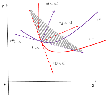
Figure 1: Shaded region indicates the set of descent directions

From the Theorem 3.2, one may conclude that the descent direction of $\breve{F}(x,y)=[\underline{F}(x,y),\overline{F}(x,y)]$ at point $(x_{0},y_{0})$ can be determined by solving $\sum_{i=1}^{n}d_{i}\odot\breve{g}_{i}(x_{0},y_{0})\prec\breve{0}$ i.e. $\breve{g}(x_{0},y_{0})^{\prime}\odot d\prec\breve{0}$. The set of descent directions is

$$\left\{d\in\mathbf{R}^{n}:\underline{g}(x_{0},y_{0})^{\prime}d<0;\overline{g}(x_{0},y_{0})^{\prime}d<0\right\}.$$

In Figure 1, $C\underline{F}$ and $C\overline{F}$ are the contours of lower and upper bound functions at levels $\underline{F}(x_{0},y_{0})$ and $\overline{F}(x_{0},y_{0})$ respectively. $T\underline{F}$ and $T\overline{F}$ are the tangent lines to the contours $C\underline{F}$ and $C\overline{F}$ at $(x_{0},y_{0})$ respectively. The set of descent directions at $(x_{0},y_{0})$ is the set of vectors in $R^{2}$, which make obtuse angle with both $\underline{g}(x_{0},y_{0})$ and $\overline{g}(x_{0},y_{0})$. This is the shaded region in Figure 1.

4 Descent direction and generating descent sequence

Selection of suitable descent direction plays an important role while developing an efficient numerical algorithm for minimizing a real valued function $f(x)$. Objective of this section is to develop a descent sequence $\breve{F}(x^{k})$ with respect to the interval ordering $\preceq$, staring at an initial point $x^{0}$. For the descent direction $d^{k}\in\mathbf{R}^{n}$ at $x^{k}$ of $\breve{F}(x)$, $\breve{F}(x^{k+1})\preceq\breve{F}(x^{k})$ holds causing reduction on lower and upper function simultaneously. Here $x^{k=1}=x^{k}+\alpha_{k}d^{k}$, where $\alpha_{k}>0$ is the step length at $x^{k}$ in the descent direction $d^{k}$, selected in such a way that $\breve{F}(x^{k+1})\preceq\breve{F}(x^{k})$ holds. This process terminates at a point $x^{*}$, when either $\alpha_{k}=0$ or no such descent direction exists. We say a point where no such descent direction exists as a critical point of $\breve{F}(x)$, which is defined below.

Definition 5.

A point $x^{*}$ is called a critical point of $\breve{F}$ if $\nexists\leavevmode\nobreak\ d\in\mathbf{R}^{n}\mbox{ such that}\leavevmode\nobreak\ \leavevmode\nobreak\ p^{T}d<0\leavevmode\nobreak\ \leavevmode\nobreak\ \forall\leavevmode\nobreak\ p\in\breve{g}(x^{*})$ .

Remark 1.

Weak efficient solution of the optimization problem $\min_{x\in R^{n}}\breve{F}(x)$ is a critical point of $\breve{F}(x)$. For a detailed study of weak efficient solution, the readers may see [2] and [14].

Following results are studied in this direction, which may be considered as a stepping stone for generating descent sequence.

Theorem 4.1.

Let $\breve{F}:\Omega\rightarrow K(\mathbf{R})$ be differentiable such that $0\notin int(\breve{g}_{i}(x))\leavevmode\nobreak\ \forall i=1,2,\cdots,n$. Then $\overline{d}$ is a descent direction at $x$ where $\overline{d}_{i}\in\ominus_{M}\breve{g}_{i}(x)$ for each $i=1,2,\cdots,n$ .

Proof.

Since $0\notin int(\breve{g}_{i}(x))\forall i=1,2,\cdots,n$, either $\frac{\partial\breve{F}}{\partial x_{i}}\succeq\breve{0}$ or $\frac{\partial\breve{F}}{\partial x_{i}}\preceq\breve{0}\forall i=1,2,\cdots,n$.
Since $\overline{d}_{i}\in\ominus_{M}\breve{g}_{i}(x)$ for each $i=1,2,\cdots,n$, so $d_{i}\geq 0$ if $\frac{\partial\breve{F}}{\partial x_{i}}\preceq\breve{0}$ and vice versa.
So, $\sum_{i=1}^{n}\overline{d}_{i}\odot\frac{\partial\breve{F}(x)}{\partial x_{i}}\prec\breve{0}$.
Therefore using Theorem 3.2, $\overline{d}$ is descent direction at $x$. ∎

Remark 2.

From the above theorem the following results can be concluded.

• For a descent direction $\overline{d}$, since $\overline{d}_{i}\in\ominus_{M}\breve{g}_{i}(x)=[-\overline{g}_{i}(x),-\underline{g}_{i}(x)]$ for each $i=1,2,\cdots,n$ , each $d_{i}$ can be written as $d_{i}=-\overline{g}_{i}(x)+t_{i}(\overline{g}_{i}(x)-\underline{g}_{i}(x))$ for each $t_{i}\in[0,1]$.

• If $\exists$ some $i$, for which $0\in int(\breve{g}_{i}(x))$, then it may not guarantee that $\overline{d}$ is a descent direction at $x$. In that case for preserving descent property one may choose $\overline{d}_{i}=0$ for those $i$.

Generating a descent sequence of interval function

For generating descent sequence of intervals $\{\breve{F}(x^{k})\}$ satisfying $\breve{F}(x^{k+1})\preceq\breve{F}(x^{k})$ and
$x^{k+1}=x^{k}+\alpha_{k}d^{k}$, selection of $\alpha_{k}$ and suitable stopping condition play important role. The iterative process will be stopped at critical point. Therefore a tolerance level $\epsilon>0$ can be fixed for $\parallel d^{k}\parallel$ as a breaking condition. Here exact line search technique for real valued functions is used for step-length selection in this iterative process, which is explained below.
Suppose $\underline{\alpha}_{k}=\arg\leavevmode\nobreak\ \underset{\alpha>0}{\min}\underline{F}(x^{k}+\alpha d^{k})$ and
$\overline{\alpha}_{k}=\arg\leavevmode\nobreak\ \underset{\alpha>0}{\min}\overline{F}(x^{k}+\alpha d^{k})$ . Choose

$$\alpha_{k}=\min\{\underline{\alpha}_{k},\overline{\alpha}_{k}\}$$ (6)

along the descent direction $\{d^{k}\}$. In particular if $\underline{F}(x^{k}+\alpha d^{k})$ and $\overline{F}(x^{k}+\alpha d^{k})$ are convex functions in $\alpha$ then $\underline{\alpha}_{k}=\min\{\alpha>0:\underline{g}(x^{k}+\alpha d^{k})^{\prime}d^{k}=0\}$ and
$\overline{\alpha}_{(k)}=\min\{\alpha>0:\overline{g}(x^{k}+\alpha d^{k})^{\prime}d^{k}=0\}$
The above theoretical development is summarized in following steps.

1. Fix tolerance level $\epsilon$, initialize $k=0$, $x^{0}$, $\alpha_{0}$, fix $t_{i}\in$ rand $[0,1]$.

2. Choose $\overline{d}_{i}(t)$ according to Remark 2.

3. Select suitable step length $\alpha_{k}$ according to (6).

4. $x^{k+1}=x^{k}+\alpha_{k}\overline{d}^{k}$.

5. Check if $\parallel\overline{d}^{k+1}\parallel<\epsilon$, stop. Otherwise $k:=k+1$.

The above steps can be verified with the following example. In this example a descent sequence is generated and critical point is verified.

Example 1.

Consider
$\breve{F}(x_{1},x_{2})=[2,4]x_{1}^{2}\oplus[2,3]x_{1}x_{2}\oplus[1,2]x_{2}^{2}\oplus[1,2]x_{1}\ominus_{M}[1,3]x_{2}$.

$\breve{F}(x_{1},x_{2})=\begin{cases}\left[2x_{1}^{2}+2x_{1}x_{2}+x_{2}^{2}+x_{1}-x_{2}\right.\vee\\ \left.4x_{1}^{2}+3x_{1}x_{2}+2x_{2}^{2}+2x_{1}-3x_{2}\right];\\ \text{ if }x_{1}\geq 0,x_{2}\geq 0\\ \left[2x_{1}^{2}+3x_{1}x_{2}+x_{2}^{2}+2x_{1}-x_{2}\right.\vee\\ \left.4x_{1}^{2}+2x_{1}x_{2}+2x_{2}^{2}+x_{1}-3x_{2}\right];\\ \text{ if }x_{1}\leq 0,x_{2}\geq 0\\ \left[2x_{1}^{2}+2x_{1}x_{2}+x_{2}^{2}+2x_{1}-3x_{2}\right.\vee\\ \left.4x_{1}^{2}+3x_{1}x_{2}+2x_{2}^{2}+x_{1}-x_{2}\right];\\ \text{ if }x_{1}\leq 0,x_{2}\leq 0\\ \left[2x_{1}^{2}+3x_{1}x_{2}+x_{2}^{2}+x_{1}-3x_{2}\right.\vee\\ \left.4x_{1}^{2}+2x_{1}x_{2}+2x_{2}^{2}+2x_{1}-x_{2}\right];\\ \text{ if }x_{1}\geq 0,x_{2}\geq 0\end{cases}$

$\nabla\breve{F}(x_{1},x_{2})=\begin{cases}\begin{pmatrix}[4x_{1}+2x_{2}+1\vee 8x_{1}+3x_{2}+2]\\ [2x_{1}+2x_{2}-1\vee 3x_{1}+4x_{2}-3]\end{pmatrix};\\ \text{ if }x_{1}\geq 0,x_{2}\geq 0\\ \begin{pmatrix}[4x_{1}+3x_{2}+2\vee 8x_{1}+2x_{2}+1]\\ [3x_{1}+2x_{2}-1\vee 2x_{1}+4x_{2}-3]\end{pmatrix};\\ \text{ if }x_{1}\leq 0,x_{2}\geq 0\\ \begin{pmatrix}[4x_{1}+2x_{2}+2\vee 8x_{1}+3x_{2}+1]\\ [2x_{1}+2x_{2}-3\vee 3x_{1}+4x_{2}-1]\end{pmatrix};\\ \text{ if }x_{1}\leq 0,x_{2}\leq 0\\ \begin{pmatrix}[4x_{1}+3x_{2}+1\vee 8x_{1}+2x_{2}+2]\\ [3x_{1}+2x_{2}-3\vee 2x_{1}+4x_{2}-1]\end{pmatrix};\\ \text{ if }x_{1}\geq 0,x_{2}\leq 0\\ \end{cases}$

Selection of descent direction at $(1,-1)$.
Here $\nabla\breve{F}(1,-1)=\begin{pmatrix}[2,8]&[-3,-2]\end{pmatrix}$.
$\overline{d_{1}}=-8+6t_{1}$, $\overline{d_{2}}=2+t_{2}$, with $t_{1},t_{2}\in[0,1]$. Choose $t_{1}=\dfrac{5}{6}$ and $t_{2}=0$. Therefore $\overline{d}=\begin{pmatrix}-3\\ 2\end{pmatrix}$. Then $\sum_{i=1}^{2}\overline{d}_{i}\odot\breve{g}_{i}(1.-1)=[-30,-10]\prec\breve{0}$. From Theorem 3.2, $\overline{d}$ is a descent direction at $(1,-1)$.

In this example a descent sequence of intervals $\{\breve{F}(x^{k})\}$ is generated starting with randomly chosen initial point. At every iteration, $\alpha_{k}$ is selected according to (6). $\overline{d}^{k}$ is determined using Remark 2. All the iterations are summarized in the following table.

Table 1: Iterations with $x^{0}=(1,1)^{\prime}$

$k$	$x^{k}$	$\breve{F}(x^{k})$	$\overline{d}^{k}$	$\alpha_{k}$
$0$	$(1.00000,1.00000)$	$[5.00000,8.00000]$	$(-13.00000,-4.00000)$	$0.10703$
$1$	$(-0.39141,0.57188)$	$[-1.90307,-0.77751]$	$(-0.58438,1.88672)$	$0.37676$
$2$	$(-0.61157,1.28271)$	$[-2.63791,-1.06984]$	$(-1.11913,-0.34227)$	$0.09160$
$3$	$(-0.71409,1.25136)$	$[-2.69151,-1.16687]$	$(-0.64637,-0.00000)$	$0.00801$
$4$	$(-0.71926,1.25136)$	$[-2.69162,-1.17016]$	$(-0.00000,-0.00000)$	$-$

From the Table 1, one may observe that $\breve{F}(x^{4})\preceq\breve{F}(x^{3})\preceq\breve{F}(x^{2})\preceq\breve{F}(x^{1})\preceq\breve{F}(x^{0})$. The iterative process terminates at $x^{4}$ since $\parallel\overline{d}^{k}\parallel<\epsilon$ where $\epsilon=10^{-5}$.

Justification of critical point:
To justify $x^{4}=(-0.71926,1.25136)$, generated in Table 1 as a critical point, from Definition 5, it is enough to show that $\sum_{i=1}^{2}d_{i}\odot\breve{g}_{i}(x^{4})\prec\breve{0}$ has no solution for any non zero $d\in\mathbf{R}^{2}$. $\breve{g}(x^{4})=\begin{pmatrix}[-2.25136,2.87704]&[-0.65506,0.56692]\end{pmatrix}$. Therefore the interval inequality will be

$$d_{1}\odot[-2.25136,2.87704]\oplus d_{2}\odot[-0.65506,0.56692]\prec\breve{0}.$$

The above inequality can be reduced to two different system of inequalities (in real form) for different signs of $d_{1}$ and $d_{2}$.
Case 1: $d_{1}$ and $d_{2}$ are of same sign.
Therefore either $d_{1}\geq 0$, $d_{2}\geq 0$ or $d_{1}\leq 0$, $d_{2}\leq 0$ with $(d_{1},d_{2})\neq(0,0)$. In that case the above interval inequality reduces to the following system of inequalities.

$$-2.25136d_{1}-0.65506d_{2}<0$$

$$2.87704d_{1}+0.56692d_{2}<0$$

For $d_{1}\geq 0$, $d_{2}\geq 0$, the first inequality holds but the second one doesn’t hold.
The second inequality satisfies the condition $d_{1}\leq 0$, $d_{2}\leq 0$ but the first one does not. Thus this system has no solution.

Case 2: $d_{1}$ and $d_{2}$ are of opposite sign.
Therefore either $d_{1}\geq 0$, $d_{2}\leq 0$ or $d_{1}\leq 0$, $d_{2}\geq 0$ with $(d_{1},d_{2})\neq(0,0)$. In that case the above interval inequality reduces to the following system of inequalities.

$$2.87704d_{1}-0.65506d_{2}<0$$

$$-2.25136d_{1}+0.56692d_{2}<0$$

Here the first inequality holds for $d_{1}\leq 0$, $d_{2}\geq 0$ but the second inequality doesn’t hold for the same condition. Similarly in case of $d_{1}\geq 0$, $d_{2}\leq 0$, second inequality holds but the second inequality cannot hold. Hence the above system has no solution.

From the above cases we can conclude that $\nexists$ non zero $d\in\mathbf{R}^{2}$ such that $\sum_{i=1}^{2}d_{i}\odot\breve{g}_{i}(x^{4})\prec\breve{0}$. Hence $x^{4}$ is a critical point of $\breve{F}$.

Since $\breve{F}(x)$ is a set valued mapping so critical point of $\breve{F}(x)$ is not unique. Starting with different initial points one may have different critical points.

5 Conclusion and future scope

The set of intervals is partially ordered. So it is not always easy to create a descent sequence for any general interval valued function. Objective of this article is to develop an iterative process to construct a descent sequence of intervals which provides a critical point of a function with bounded parameters as intervals. Some natural questions raise after the theoretical discussions of this article. Though $\{\breve{F}(x^{k})\}$ is a descent sequence of intervals, convergence of $\{x^{k}\}$ to the critical point can be guaranteed only with several assumptions on $\breve{F}$. This part is not studied here and kept for future research. The article focuses only on the iterative process. Exact line search technique is used to decide the step length. Determination of suitable step length satisfying conditions (6) is cumbersome for complex functions. There are several inexact line search methods for selection of step length, which may be used to justify the convergence, which remains the scope of the present contribution.

References

- Bhurjee and Padhan [2016] Ajay Kumar Bhurjee and Saroj Kumar Padhan. Optimality conditions and duality results for non-differentiable interval optimization problems. Journal of Applied Mathematics and Computing, 50(1-2):59–71, 2016.
- Bhurjee and Panda [2012] Ajay Kumar Bhurjee and Geetanjali Panda. Efficient solution of interval optimization problem. Mathematical Methods of Operations Research, 76(3):273–288, 2012.
- Chalco-Cano et al. [2011] Yurilev Chalco-Cano, Heriberto Román-Flores, and María-Dolores Jiménez-Gamero. Generalized derivative and -derivative for set-valued functions. Information Sciences, 181(11):2177–2188, 2011.
- Chalco-Cano et al. [2013] Yurilev Chalco-Cano, Antonio Rufián-Lizana, Heriberto Román-Flores, and María-Dolores Jiménez-Gamero. Calculus for interval-valued functions using generalized hukuhara derivative and applications. Fuzzy Sets and Systems, 219:49–67, 2013.
- Dimitrova et al. [1992] NS Dimitrova, SM Markov, and ED Popova. Extended interval arithmetics: new results and applications. Computer Arithmetics and Enclosure Methods, pages 225–232, 1992.
- Kyurkchiev and Markov [2016] Nikolay Kyurkchiev and Svetoslav Markov. On the hausdorff distance between the heaviside step function and verhulst logistic function. Journal of Mathematical Chemistry, 54(1):109–119, 2016.
- Lupulescu [2013] Vasile Lupulescu. Hukuhara differentiability of interval-valued functions and interval differential equations on time scales. Information Sciences, 248:50 – 67, 2013.
- Markov [1977] SM Markov. Extended interval arithmetic. CR Acad. Bulgare Sci, 30(9):1239–1242, 1977.
- Markov [1979] Svetoslav Markov. Calculus for interval functions of a real variable. Computing, 22(4):325–337, 1979.
- Markov [1999] Svetoslav Markov. An iterative method for algebraic solution to interval equations. Applied Numerical Mathematics, 30(2):225 – 239, 1999.
- Markov [2000] Svetoslav Markov. On the algebraic properties of convex bodies and some applications. Journal of Convex Analysis, 7:129–166, 2000.
- Markov [2004] Svetoslav Markov. On quasilinear spaces of convex bodies and intervals. Journal of Computational and Applied Mathematics, 162(1):93 – 112, 2004.
- Markov [2005] Svetoslav Markov. Quasilinear spaces and their relation to vector spaces. Electronic Journal on Mathematics of Computation, 2:1–21, 2005.
- Osuna-Gómez et al. [2015] R. Osuna-Gómez, Y. Chalco-Cano, B. Hernández-Jiménez, and G. Ruiz-Garzón. Optimality conditions for generalized differentiable interval-valued functions. Information Sciences, 321:136–146, 2015.
- Roumen Anguelov [2006] Blagovest Sendov Roumen Anguelov, Svetoslav Markov. The set of hausdorff continuous functions— the largest linear space of interval functions. Reliable Computing, 12:337–363, 2006.
- Roumen Anguelov [2016] Svetoslav Markov Roumen Anguelov. Hausdorff continuous interval functions and approximations. In Scientific Computing, Computer Arithmetic, and Validated Numeric, pages 3–13, Cham, 2016. Springer International Publishing.
- Stefanini and Bede [2009] Luciano Stefanini and Barnabas Bede. Generalized hukuhara differentiability of interval-valued functions and interval differential equations. Nonlinear Analysis: Theory, Methods & Applications, 71(3):1311–1328, 2009.
- Stefanini et al. [2008] Luciano Stefanini et al. A generalization of hukuhara difference for interval and fuzzy arithmetic. Soft Methods for Handling Variability and Imprecision, in: Series on Advances in Soft Computing, 48, 2008.