Log Complex Color for Visual Pattern Recognition of Total Sound

Abstract

While traditional audio visualization methods depict amplitude intensities vs. time, such as in a time-frequency spectrogram, and while some may use complex phase information to augment the amplitude representation, such as in a reassigned spectrogram, the phase data are not generally represented in their own right. By plotting amplitude intensity as brightness/saturation and phase-cycles as hue-variations, our complex spectrogram method displays both amplitude and phase information simultaneously, making such images canonical visual representations of the source wave. As a result, the original sound may be precisely reconstructed (down to the original phases) from an image, simply by reversing our process. This allows humans to apply our highly developed visual pattern recognition skills to complete audio data in new way. (Published after peer review in 2016 as Audio Engineering Society Convention 141 paper 9647; now the subject of US patent 10,341,795.)

I Introduction

While some current audio visualization methods use the complexFitz and Fulop (2009); Fulop and Fritz (2006); Xiao and Flandrin (2007); Flandrin and Borgnat (2010); Flandrin et al. (2003) fast Fourier transform (FFT) components to augment the accuracy of (real) amplitude readings, they tend to be highly application-specific, and do not appear concerned with the significance of generalized, total-sound analysis, by which simultaneous display of both amplitude and phase data in each pixel provides a canonical means of recording, analyzing, cataloguing, and displaying more sound than humans are generally considered capable of hearing. Our work has been to develop an efficient and robust real-time method of viewing total sound spectrographs that incorporates log-intensity (for improved dynamic range) amplitude-visualization combined with chroma-likeBartsch and Wakefield (2001); Cho et al. (2010); Harte and Sandler (2005) phase-visualization. By simultaneously displaying both real and imaginary FFT data-sets, we ensure that an image contains all the information of the original source, which means it is always possible to recover the original sound from any image generated with this method, down to the original phases. This opens the possibility of alternative data storage techniques, novel cataloguing methods such as visual sound field-guides (which, when combined with a mobile real-time visualization app could allow for live imitation-feedback), improved sound-availability for the hearing-impaired, and more. Additional modifications that include, e.g., Grand Staff musical overlay and/or stereo versions for wearable devices could help music readers without specific technical backgrounds and/or sensory capabilities to make sense of such total-sound visualizations. The ever-increasing capability of modern mobile devices can already support implementation of this visualization method, leveraging their wide distributionWu and Chen (2015) as well as their pre-installed microphones, color displays, and processing speedsUkidave et al. (2014).

II Methods

Our experience studying spatial periodicities in nanocrystalline solidsFraundorf (2004); Fraundorf et al. (2007, 2006); Cowtan has shown us the utility of representing both amplitude and phase with a single pixel, since condensed matter crystals contain periodicities in two and three spatial dimensions, and so require higher dimensional FFTs rather than the one time-dimension periodicities involved in audio analysis. By applying this visualization method to audio signals, we can display the complete, complex FFT of a given time-slice as a single column of pixels, allowing the horizontal axis to remain available for sequential slices in the time domain.

In contrast to current audio visualization methods like traditional spectrograms, reassigned spectrogramsFitz and Fulop (2009); Fulop and Fritz (2006); Xiao and Flandrin (2007); Flandrin and Borgnat (2010); Flandrin et al. (2003), constant-Q transforms (CQTs)Brown (1991, 1992); Velasco et al. (2011); Schorkhuber and Klapuri (2010), and chroma featuresBartsch and Wakefield (2001); Cho et al. (2010); Harte and Sandler (2005) which use various techniques to optimize amplitude visualization, we explore here only a simpler scheme based on complex FFTs that simultaneously displays the amplitude and phase information associated with each pixel. As in many other applicationsPucik et al. (2014); Bank (2011); Harma and Paatero (2001); Jin et al. (2012), not least of which is the traditional, Western musical notationMason (1960); Sundberg (1982); Cazden (1958), we optionally adopt logarithmic scaling of the frequency axis since on it octaves and harmonics are equally spaced. While techniques like reassigned spectrograms utilize the imaginary part of the Fourier transform to enhance accuracy of particular amplitude and harmonic representationsFitz and Fulop (2009); Fulop and Fritz (2006); Xiao and Flandrin (2007); Flandrin and Borgnat (2010); Flandrin et al. (2003), and chroma visualizations show periodic changes in tone as hue-variationsBartsch and Wakefield (2001); Cho et al. (2010); Harte and Sandler (2005), our method simultaneously displays both real and imaginary Fourier data to produce a canonical view of total sound. By showing Fourier coefficient amplitude as the brightness/saturation of the associated pixel, and Fourier phase as hue, each pixel simultaneously represents both real and imaginary components of a complex Fourier coefficient.

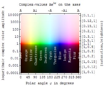
Figure 1: Logarithmic complex-color key in polar coordinates with amplitude on the logarithmic vertical axis and imaginary phase angle $\phi$ on the linear horizontal axis.

On a linear frequency scale, log-color phase representation begins with each complex Fourier coefficient being converted to a color according to Fig. 1. In such a representation, the hue is determined by the coefficient’s phase angle whereas the brightness/saturation is determined by the logarithm of the intensity of the coefficient. As seen in Fig. 1, Fourier-coefficient phase-shifts in one direction result in a red-to-green-to-blue (RGB) sequence, whereas movement in the opposite direction results in a red-to-blue-to-green (RBG) sequence. Since the frequency scale is linear, the only interpolation involved is that which maps the saturation and brightness from a linear to a logarithmic intensity scale (vertical axis of Fig. 1). By plotting the log of the intensity rather than only the intensity, some fine details are sacrificed in order to provide conventionalGiannoulis and Klapuri (2013) improvements in dynamic range. Hue, saturation, and brightness parameters between 0 and 1 are determined by equations (1), (2), and (3), respectively. This reversible mapping between complex-number absolute-value and pixel-color thereby trades contrast for dynamic range.

$$\text{hue}=\frac{\phi}{2\pi}$$ (1)

$$\text{saturation}=\begin{cases}1&\mbox{ if }A\leq 1\\ \frac{1}{1+\ln[A]}&\mbox{ if }A>1\end{cases}$$ (2)

$$\text{brightness}=\begin{cases}\frac{1}{1-\ln[A]}&\mbox{ if }A\leq 1\\ 1&\mbox{ if }A>1\end{cases}$$ (3)

In order to achieve the benefits of the log-frequency scale from equally spaced samples in the timedomain, the linear-frequency data must be transformed, limiting the retention of some detailed sound information in favor of a more robust visual representation. In particular, since the transformation from linear- to log-frequency expands the lowerfrequency coefficients and compresses the higherfrequency coefficients along the vertical axis, the lower-frequency coefficients (those below about 1200 Hz) require interpolation to sufficiently inform the brightness values for the multiple rows of a single coefficient. In contrast, the higher-frequency coefficients are under-sampled so that only coefficients closest to display-rows are represented. This optional nonlinear transformation of the frequency axis allows the discrete time-frequency spectrogram to be “warped” (different frequencies stretched or compressed differently, but frequencyorder preserved) without being “scrambled” (order of represented frequencies not preserved)Oppenheim and Johnson (1972), making it more amenable to visual pattern recognition techniquesPucik et al. (2014); Harma and Paatero (2001); Jin et al. (2012); Giannoulis and Klapuri (2013).

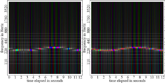
Figure 2: Rectangular (left) and polar (right) complex-color log-frequency interpolation of Fourier coefficients for a 10 percent frequency-modulated tone centered around 256 Hz.

The log-frequency display is then rendered by first completing the linear-frequency counterpart as described above and then by mapping the vertical axis to a log-frequency scale. At lower frequencies, this requires interpolation between complex-valued coefficients, for which there are two obvious methods. While both polar and rectangular interpolation routines were applied to this task, rectangular interpolation (Fig. 2a) was found to be preferable to polar interpolation (Fig. 2b). This is because the rectangular approach produces a plot that can be interpreted based on existing knowledge of phases and coefficient centers, whereas the polar approach contains an inherent ambiguity in phase assignment. The newly interpolated phase-angles are then represented as colors as shown in Fig. 1.

Since each Fourier coefficient corresponds to a frequency range determined by the FFT size, a coefficient “center” is where a linear coefficient index plots on the log-frequency scale. Since tiny changes in amplitude can be detected by examining more-sensitive phase-variations, mapping Fourier phase to hue allows frequency-variations well below the resolution allowed by a typical FFT size to be visualized from one time-slice to the next as colored stripes. In this way, rougher frequency data are shown with brightness/saturation, while the finer details are represented in color. Assuming a sampling rate of 44.1 kHz and a 2048 FFT size, the separation of coefficient centers is 44100/2048   21.533 Hz.

At various points between coefficient centers, rectangular interpolation results in zero-amplitude phase-inversions. During these transitions, the interpolated phases switch from being above the center of the lower coefficient to being below the center of the higher coefficient, or vice versa, at which point the Fourier phase undergoes an inversion. At these intersections, the interpolated amplitudes reach zero before immediately becoming positive again. The effect is that black lines appear between coefficient centers with alternating color rotations on either side. Such black lines are artifacts of the rectangular phase-interpolation routine, and, as an exception, do not actually correspond to zerointensities in the input signal. This effect can be seen in practice in Fig. 2a.

III Results

Realizations of this log-color visualization method in HTML5/JavaScriptFraundorf and Wedekind (2016) have been shown to process and render audio signals on a variety of hardware platforms in $\simeq\frac{1}{3}$ the time necessary to maintain real-time synchronization. Since this method for showing variation in phase among Fourier coefficients allows for the representation of a complex number by a single pixel, the entire FFT can be conveniently displayed as a vertical line of colored pixels with the brightness corresponding to the log of the intensity of the Fourier coefficient and the hue corresponding to the coefficient-phase. In the time direction, steady variations in Fouriercoefficient phase at the onset of each time-slice are seen as colored stripes, with stripes of opposing sequence (RGB vs. RBG) occupying opposite sides of the zero-amplitude lines. When the oscillation frequency is below the center of a coefficient, the hue alternates in the RBG direction, and when the oscillation frequency is above a Fourier-coefficient center, the hue alternates in the RGB direction, as seen in Fig. 2a. For a static tone, the frequency misalignment, in Hertz, with the Fourier-coefficient hardware-reference-frequency was found to be equal to the number of color-cycles in a one-second interval.

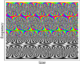
Figure 3: Composite beat-schematic, with 128 vertical time-slices arrayed across the horizontal axis, and 4 center-to-center frequency-coefficients on the vertical axis.

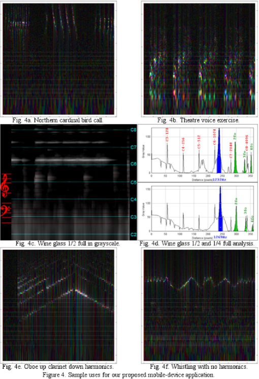
Figure 4: Sample uses for our proposed mobile-device application.

Whenever the phase is centered on the Fourier coefficient, the hue remains constant, which allows highly accurate, well-centered data points to be easily distinguished and isolated even in real-time. In fact, the color-oscillations have a period inversely proportional to the frequency offset from the coefficient center, just as do amplitude beats used to tune woodwind instruments (see Fig. 3). Each frequency-coefficient in Fig. 3 is divided into 25 lines with randomized phase-offsets to highlight beat-oscillations as a function of the frequencyoffset from the coefficient-center (solid color lines). The central dashed line in Fig. 3 marks the center of one frequency coefficient, with top and bottom boundaries 1/8th of the height away in each direction. The top 5/8ths of the plot show color phase-beats with respect to coefficient center, while the bottom 3/8ths shows monochrome amplitudebeats with respect to a coefficient-centered note.

IV Discussion

The connection of technologies like microphones, digital displays, and computing power with currently-existing, globally-interconnected, wireless networks of highly-portable devices provides a historically unique opportunity to drastically expand the scope of applications for visual audio analysis. In addition, versatile phase-sensitive audio-analysis applications incorporating both modern (logfrequency) and traditional (Grand Staff) optimizations for enhancing visual pattern recognition can provide a meaningful (or at least relatable) basis from which anyone with experience reading music can make interpretations of phasedetailed audio data.

Several examples of applications involving these features are illustrated in Fig. 4. In Figs. 4a-f the vertical axis is frequency and the horizontal axis is time.

The inclusion of relevant sound images in text- or print-based media (such as bird-sound field-guides as suggested by panel in Fig. 4a) would allow users without appropriate hardware to take advantage of this technology by applying independent patternrecognition analysis to existing sound-images. Moreover such printed images may be used in conjunction with, for example, a mobile-friendly analysis-app to visually compare and classify live captures with sound-visuals of known origin.

A real-time picture of incoming-sound (as in the theatre voice example of Fig. 4b) can empower voice imitators as well, even those who are hearingimpaired. Figs. 4c and 4d illustrate the utility for home experimenters in the spirit of Google’s Science Journal app, while Figs. 4e and 4f illustrate visual comparison of musical instrument harmonics.

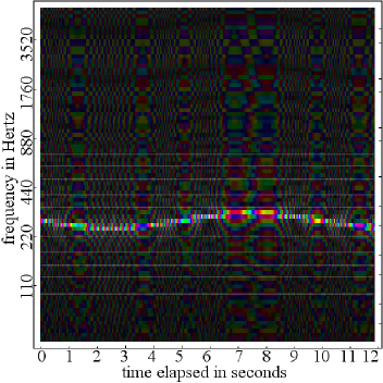
Figure 5: Half-note log-frequency rendition of a 10% frequency-modulated tone centered around 256 Hz.

In addition to displaying data on the complete sound wave, a generated image can be reverse-processed to recover the original signal, including the original phases imparted by the interference of the digital detector with the source wave, which contain information like relative angle to direction of sourcewave propagation, etc. While CQTs have also been shown to be invertibleVelasco et al. (2011), they do not display phase information explicitly and generally require additional computational resources compared to the discrete FFTSchorkhuber and Klapuri (2010). Since musical notation provides a practical reference, and since each pixel can be mapped back to the original sound, both human imitation and recovery to audio are also possible. Other modifications, such as adjustment of the frequency axis so Fourier coefficients match frequencies of particular tuning standards, could be used to readily display whether a note is in appropriate tune, or if not, whether it is sharp or flat and by precisely how much. Such note-specific applications would be completely accessible to anyone who reads music, and would incorporate a new class of potential users of technically sophisticated audio analysis software.

Finally, our browser implementations are only one facet of this development. More specialized implementations, e.g., in hardware instead of software will open the door to other uses. For instance, by doing a separate transform for each half-note in a log-frequency display, one can avoid all interpolation artifacts and put any sound into playable music notation (see Fig. 5). In fact, a single 12 second multi-octave chromatic scale could be used to quantify the tuning state of all notes on a piano.

V Summary

By enabling sound visualization that includes source-detector phase-interference in a convenient, familiar, and portable format, this combination of processing and display techniques opens the door for improved accuracy in sound measurement and analysis in a plethora of new and diverse environments and applications. With further development of robust audio visualization software in parallel with semiconductor technology, the general public will soon have access to a growing variety of specialized, phase-interferometric tools to record, analyze, and recreate sounds on an increasingly real-time basis. As software continues to be developed, applications which take advantage of traditional musical notation will always have the advantage of wider accessibility by the general public, as well as additional potential for musical reproduction and conceptual reference. Furthermore, the ability to record and analyze audio in a visual form that retains precise information regarding the physical orientation of the actual sound wave in space relative to the detector that recorded it marks an important step in detailed sound-feature analysis.