Dynamical complexity measure to distinguish organized from disorganized dynamics

Abstract

We propose a metric to characterize the complex behavior of a dynamical system and to distinguish between organized and disorganized complexity. The approach combines two quantities that separately assess the degree of unpredictability of the dynamics and the lack of describability of the structure in the Poincaré plane constructed from a given time series. As for the former, we use the permutation entropy $S_{\rm p}$, while for the later, we introduce an indicator, the structurality $\Delta$, which accounts for the fraction of visited points in the Poincaré plane. The complexity measure thus defined as the sum of those two components is validated by classifying in the ($S_{\rm p}$,$\Delta$) space the complexity of several benchmark dissipative and conservative dynamical systems. As an application, we show how the metric can be used as a powerful biomarker for different cardiac pathologies and to distinguish the dynamical complexity of two electrochemical dissolutions.

I Introduction

Recent decades have witnessed a considerable growth of the science of complexity, devoted to understanding the collective behavior of systems, regardless of their physical, biological, or social natureAdami et al. (2000); Perkiömäki et al. (2005); Regev (2006); Sabeti et al. (2009); Flack and Krakauer (2011); Aquino et al. (2017); Pozo et al. (2017). Much of the research has focused on defining multiple metrics to classify and quantify complex dynamics involving many variables Lloyd (2001). First attempts were made by extending information theory to dynamical systems Kolmogorov (1958); Sinai (1959) and adapting Shannon’s entropy Shannon (1948) to statistically estimate the apparent randomness present in deterministic chaotic dynamics. As long as the Jaynes’ principle of maximum entropy Jaynes (1957) is properly applied Skilling and Bryan (1984); Berger et al. (1996); Larivee and Brown (1992); Fresnel et al. (2015), the Shannon’s entropy informs about the rate at which information is produced and, consequently, it is a measure of a system’s predictability. However, as Weaver posited Weaver (1948), there are two classes of complexity: disorganized and organized. We will refer here to organized (disorganized) dynamics when its Poincaré section is describable (indescribable). While the former can be tackled using the methods of statistical mechanics and probability theory, the latter cannot be fully understood using statistics alone as it involves considerable large number of variables that are interrelated.

Entropic metrics work well as indicators of the level of unpredictability and randomness, but fail to correctly capture the existence of inter-dependencies or structure among the system’s components Huberman and Hogg (1986). This drawback is mostly due to the commonly accepted standard that both maximally random and perfectly ordered systems do not exhibit any degree of structural organization Huberman and Hogg (1986) and, therefore, a measure quantifying their degree of complexity should be minimal Feldman and Crutchfield (1998) without any distinction between the two cases. Among several approaches proposed for detecting an underlying structure, are those called statistical complexity measures, which account for the graph complexity of the representation of symbolic sequences as trees Huberman and Hogg (1986); Crutchfield and Young (1989), or in terms of disturbance from the equiprobable distribution of the accessible states of the system R. López-Ruiz and Calbet (1995); Martin et al. (2003). However, these strategies, although using combinations of different indicators, rely on the same background information: the probability of different symbolic sequences. Thus, for instance, they are not able to distinguish a fully developed chaos from a stochastic dynamics as in both cases the probabilities are uniformly distributed.

Here we provide a dynamical complexity measure $C_{\rm D}$ which is able to rank both the degree of unpredictability and indescribability of a structure present in a process. It combines the Shannon entropy as indicator of the unpredictability with the density of points in the Poincaré plane as an alternative metric of organization. Our measure is designed to be zero for a fully predictable and perfectly ordered dynamics, one for a nonpredictable but organized dynamics and a value of two for a nonpredictable disorganized one. We illustrate the capabilities of our measure introduced in Sec. II in several dissipative and conservative dynamical systems whose complex behavior can be accessed by tuning a system’s parameter (Sec. III). Finally, in Sec. IV, we show how it can be used to compare the complex dynamics of two electrochemical dissolutions and as a biomarker for different cardiac diseases directly obtained from electrocardiograms (ECGs).

II Dynamical complexity

Let us start by showing how the family of the extensively used entropy-based statistical complexity measures $C_{\rm S}$, first introduced by López-Ruiz et al. R. López-Ruiz and Calbet (1995) and later on improved by Martin et al Martin et al. (2003), fails to detect the organized complexity underlying the paradigmatic logistic map. $C_{\rm S}$ is usually defined as $C_{\rm S}=QH$, where $Q$ stands for the so-called disequilibrium, which quantifies how far is the probability distribution of a given process from the uniform one, and $H$ is the corresponding normalized Shannon entropy. Such a factorization ensures that $C_{\rm S}$ vanishes for perfect order ($H=0$) and maximal randomness ($Q=0$), and it is expected to capture a wide range of complex behaviors in between. However, when we compare a uniform white noise $\zeta_{n}\in[0;1]$ with the logistic map

$$x_{n+1}=\mu x_{n}(1-x_{n})$$ (1)

whose behavior $x_{n}\in[0;1]$ depends on the parameter $\mu$, we find a clear example where the statistical complexity measure $C_{\rm S}$ is not performing properly, in particular when the logistic map exhibits fully developed chaotic behavior for $\mu=4$. Figure 1 shows an illustrative characterization of the two dynamics by means of first-return maps (top panels) and time series (bottom panels). The time series of both dynamics look quite alike, actually characterized by an almost flat histogram for the symbolic sequences Letellier (2008), which yields to null values of $C_{\rm S}$. However, their respective first-return maps reveal a well-defined underlying structure for the chaotic dynamics [top panel in Fig. 1(a)] while the noise fills the whole available state space [top panel in Fig. 1(b)] with no signs of dynamical organization.

Figure 1: (Upper row) First-return maps for (a) logistic map with $\mu=4$ and (b) uniform white noise with the same amplitude. (Bottom row) Characteristic time series for the same both examples. For the logistic map, the first return map shows the generating partition $x_{\rm c}=\frac{1}{2}$ and the corresponding symbolic dynamics.

Therefore, we need a marker capable of discriminating the presence of a structured dynamics, easily describable. The Shannon entropy already quantifies how the structure — when it exists — is visited in the state space. It must be complemented by a second marker capable of measuring how the structure fills the state space, based on the principle that the more structured the attractor is, the smaller the volume it occupies. If we choose the Poincaré section as a more reliable source to compute the entropy than the time series itself Letellier (2006), then the argument can be reformulated by stating that the smaller the fraction of boxes visited by the Poincaré section, the more constrained and organized the dynamics. In general, we will be working in a two-dimensional projection of the Poincaré section independently of the system’s dimension. For the strongly dissipative systems we investigate, the Poincaré section can be safely reconstructed from a single variable by using delay coordinates and we will therefore use the first-return map to obtain it.

To assess how a dynamics is structured in the state space, we introduce the structurality $\Delta$ index, which accounts for the fraction of visited boxes from a pixelation of the Poincaré section into $N_{\rm b}\times N_{\rm b}$ boxes, that is,

$$\Delta={\sum^{N_{\rm b}}_{i,j=1}\displaystyle\frac{v_{ij}}{N_{\rm b}^{2}}}\in[0;1]\,,$$ (2)

where $v_{ij}=1$ if the box $(i,j)$ contains at least one crossing point and $v_{ij}=0$ otherwise. To implement this definition we need first to determine the frame in which the Poincaré section is investigated. The easiest way is to construct a domain from the visited range, that is, the minimum and maximum values along the two axis of the Poincaré plane. We will refer to this frame as the renormalized frame. In some cases, as when a bifurcation diagram is investigated, it is more efficient to use a fixed frame corresponding to the most developed Poincaré section: we will designate it as a relative frame. Let $[m_{i};M_{i}]$ be the range of the $i$ axis of the chosen frame. Then we need to specify the pixelation, that is, the number $N_{\rm b}^{2}$ of boxes, and their length $l_{\rm b}$. The former can be estimated as a function of the number $N_{\rm p}$ of points in the Poincaré section as

$$N_{\rm b}\gtrsim 10\,\log_{10}N_{\rm p}\,.$$ (3)

However, as long as $N_{\rm p}$ is large enough for properly sampling the dynamics, the dependence of $\Delta$ on the pixelation settings is not critical, as we show in the Appendix. The length of each box is determined according to

$$l_{\rm b}=\frac{\lVert M_{i}-m_{i}\rVert}{N_{\rm b}}\,,$$ (4)

A lack of describability of the structure of the dynamics will be manifested by a large value of $\Delta$, while a well ordered dynamics like a period-one behavior will have $\Delta=1/N_{\rm b}^{2}\sim 0$. See the Appendix for a more elaborated discussion on this issue.

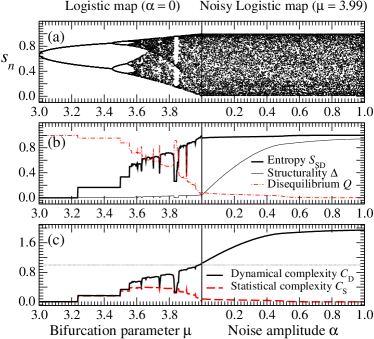
Figure 2: (a) Bifurcation diagram of the logistic map vs $\mu$ for $\alpha=0$ (left half) and vs $\alpha$ for $\mu=4$ as it is progressively replaced with noise (right half) according to Eq. (6). (b) Shannon entropy based on the symbolic dynamics $S_{\rm SD}$ (black thick line), relative structurality $\Delta$ (black thin line), and disequilibrium $Q$ (red dash-dotted line). (c) Dynamical complexity $C_{\rm D}=S_{\rm SD}+\Delta$ and statistical complexity $C_{\rm s}=S_{\rm SD}\cdot Q$. $N_{\rm p}=180,000$.

At this point, we combine into a single dynamical complexity measure $C_{\rm D}$ the two components characterizing the lack of predictability, the Shannon entropy $S_{\rm p}$, and the lack of describability, the structurality $\Delta$, as

$$C_{\rm D}=S_{\rm p}+\Delta\,,$$ (5)

where $S_{\rm p}$ is by default the permutation entropy Bandt and Pompe (2002), unless stated otherwise.

We evaluate now how $C_{\rm D}$ performs by first discussing its application to the logistic map $x_{n}$ dynamically coupled to a white uniform noise $\zeta_{n}$ as

$$s_{n}=(1-\alpha)x_{n}+\alpha\zeta_{n},$$ (6)

where $x_{n},\;\zeta_{n}\in[0;1]$ and $\alpha$ is a parameter ranging between $0$ ($s_{n}=x_{n}$, logistic map) and $1$ ($s_{n}=\zeta_{n}$, white noise). Here the Shannon entropy $S_{\rm SD}$ is based on the symbolic dynamics produced by the generating topological partition Letellier (2006) $\sigma_{i}=0$ if $s_{n}<\frac{1}{2}$ and $\sigma_{i}=1$ otherwise, which satisfies the maximum-entropy principle for the logistic map Jaynes (1957). The dynamics is thus reduced to sequences of $0$’s and $1$’s of length 6 whose frequencies of occurrence are calculated over $N_{\rm p}=180,000$.

The left half of Fig. 2(a) shows the bifurcation diagram of the noise free ($\alpha=0$) logistic map for $3\leq\mu\leq 4$, while in the right half $\mu$ is kept constant to $3.99$ and $0\leq\alpha\leq 1$, giving rise to a fully developed chaos increasingly contaminated by uniform noise of growing amplitude. In Fig. 2(b) we plot the Shannon entropy $S_{\rm SD}$, the structurality $\Delta$, and the generalized Jensen-Shannon disequilibrium $Q$ (red dash-dotted line) as proposed in Ref. Martin et al. (2003). $S_{\rm SD}$ initially increases in a stepwise form as the logistic map undergoes the period-doubling bifurcation up to a point where a much richer structure arises characterized by chaotic behavior intermingled with periodic windows in which the entropy drops accordingly to the periodicity. For $\mu=4$, the logistic map is fully chaotic, all its symbolic states are equally likely and, therefore, $S_{\rm SD}=1$, reaching the maximum lack of predictability of the system, which keeps bounded independently of the added noise intensity. However, the structurality $\Delta$ informs us about how organized is the state space: the Poincaré section of the noise-free logistic map changes from an isolated point for the period-1 cycle ($\mu=3$) to a smooth unimodal map in the unit square for the fully developed chaos [$\mu=4$, see Fig. 1(a)], yielding in every case to a very well structured dynamics with $\Delta\ll 1$, but still capturing the different degrees of chaotic behavior. When noise is added to the $\mu=4$ case [right half in Fig. 2(b)], $\Delta$ increases monotonously until it saturates when the lack of structure fills up completely the unit square and $\Delta\sim 1$. Note that, while the entropy barely changes, the relative structurality is clearly differentiating the increasing degree of disorganization of the dynamics. Regarding the disequilibrium, it behaves as expected as it is again a function of the probability of the different symbolic sequences: it is maximum for period-1 oscillations and vanishes indistinguishably for fully chaotic and stochastic dynamics. Finally, in Fig. 2(c) dynamical and statistical complexities are depicted together. While $C_{\rm S}$ exhibits the well-known behavior exclusively driven by the information contained in the entropy, $C_{\rm D}$ is able to discriminate between the different dynamical behaviors in increasing order of complexity, assigning the maximum value $C_{\rm D}=2$ to the fully unpredictable and indescribable dynamics featured by a white noise, the minimum value $C_{\rm D}=0$ to a fully predictable and describable periodic motion, and a value close to $1$ for a yet unpredictable but structured (describable) chaotic behavior.

III Benchmark systems

So far, we have illustrated the definition of our dynamical complexity measure $C_{\rm D}$ using a simple nonlinear map. To test it in a more general context of flows, we have chosen three dynamical systems whose state space range from finite to infinite dimensional and whose dynamical behavior can be varied with a parameter: (i) a 4D double-gyre conservative system Charó et al. (2019), (ii) two coupled Rössler oscillators Rössler and Ortoleva (1978), and (iii) the time delay-differential Mackey-Glass model Farmer (1982). Let us show the results before introducing each system and discuss the connection between the complexity measure and the dynamical interpretation. Figure 3 shows the evolution of the dynamical complexity and its two components, $S_{\rm p}$ and $\Delta$ versus the corresponding bifurcation parameter.

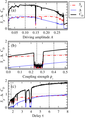
Figure 3: Evolution of the permutation entropy $S_{\rm p}$, relative structurality $\Delta$, and dynamical complexity $C_{\rm D}$ versus a bifurcation parameter for (a) the symmetrized double-gyre system, (b) a dyad of Rössler systems and (c) the delay-differential Mackey-Glass equation. Legend in (a) applies to all panels. Vertical dashed lines mark some parameter values whose dynamical regimes will be later analyzed more in detail.

The results of Figs. 2 and  3 are further explored in Fig. 4 plotting the evolution of $\Delta$ versus $S_{\rm p}$ of each system along their respective parameters. Remarkably, in this last representation the different dynamical regimes are almost exclusively distributed in three regions according to our complexity descriptor: lower-left region ($S_{\rm p},\Delta<0.5$), corresponding to a very structured and predictable behavior; lower-right region ($S_{\rm p}>0.5$, $\Delta<0.5$), structured but unpredictable behavior; and upper-right region ($S_{\rm p}$, $\Delta>0.5$) comprising unpredictable and indescribable dynamics.

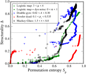
Figure 4: Permutation entropy $S_{\rm p}$ versus relative structurality $\Delta$ for the same systems and parameters as in Figs. 2 and 3.

III.1 Symmetrized double-gyre system

Conservative systems can produce chaotic as well as regular (periodic or quasi-periodic) behavior. According to the KAM theorem, only a finite fraction of the state space is visited by regular solutions which can be viewed as “islands” in a chaotic sea Hénon and Heiles (1964); Lichtenberg and Lieberman (1992). Typically, this chaotic sea is very difficult to describe and we expect to have a complexity measure ${\cal C}_{\rm D}$ close to 2 Couliette and Wiggins (2000). As an example of this class of systems, we used a recently introduced simplified model for the driven double-gyre, a typical phenomenon observed in the large-scale ocean circulation Couliette and Wiggins (2000); Shadden et al. (2005); Charó et al. (2019):

$$\begin{array}[]{l}\dot{x}=A\pi\sin[\pi(ux^{2}+x-u)]\sin(\pi y)\\[2.84544pt] \dot{y}=A\pi\cos[\pi(ux^{2}+x-u)]\cos(\pi y)\\[2.84544pt] \dot{u}=v\\[2.84544pt] \dot{v}=-\omega^{2}u\,.\end{array}$$ (7)

This is a four-dimensional conservative system where $x$ and $y$ are the variables spanning the physical space, $u$ and $v$ are variables related to the velocity field, and $A$ is the amplitude of a periodic forcing applied to the velocity field. The corresponding complexity markers are shown in Fig. 3(a) as a function of the driving amplitude $A$.

The solutions produced by this system are investigated using the Poincaré section

$${\cal P}_{\rm dg}\equiv\left\{(x_{n},y_{n})\in\mathbb{R}^{2}\leavevmode\nobreak\ |\leavevmode\nobreak\ u_{n}=0,v_{n}>0\right\}\,.$$ (8)

The main difference between a strongly dissipative system and a conservative one is that, in the former case, the Poincaré section is a uni-dimensional curve while, in the latter case it is at least a two-dimensional structure: As a consequence, the symmetrized driven double-gyre system must be investigated in a two-dimensional Poincaré section to correctly understand the organization of the chaotic sea around the regular islands. This is exhibited by the Poincaré section $\{x_{n},y_{n}\}$ in Fig. 5(a) where four large islands are observed. Since we are here concerned by the dynamical complexity computed for the chaotic sea, we selected initial conditions in the middle of the Poincaré section, a neighborhood which belongs to the chaotic sea (when it exists) for most of the parameter values used in this work.

Figure 5: Poincaré section of the symmetrized driven double-gyre system (7) for various initial conditions. The corresponding $A$ values are marked with vertical dashed lines in Fig. 3(a). Other parameter values: $\omega=\frac{\pi}{5}$.

Computations are performed with $N_{\rm p}=80,000$ and a relative frame $[-1;+1]\times[-0.5;+0.5]$. Notice that all chaotic sea would induce a renormalized frame equal to this relative frame. As shown in Fig. 3(a), this system presents high values of the Shannon entropy ($S_{\rm p}>0.7$) and structurality ($\Delta\geq 0.4$), revealing that the map is not 1D. The size of the regular islands strongly depends on the $A$-value: for instance, when $A$ increases beyond $0.1488$, the size of these islands grows with a consistent decay in the complexity, therefore reducing the visited region which results in a reduction of $\Delta$. This is well exemplified in Fig. 5(b), where the Poincaré section for $A=0.25$ shows two very large regular islands. In fact, the structurality quantifies the mixing properties of this flow: the larger $\Delta$, the greater the mixing.

III.2 A dyad of Rössler systems

The next example in Fig. 3(b) is a 6D system of two slightly mismatched chaotic Rössler oscillators — in a non phase-coherent regime — diffusively coupled through the $z$ variable. The equations are:

$$\begin{array}[]{l}\dot{x}_{1}=-y_{1}-z_{1}\\[2.84544pt] \dot{y}_{1}=x_{1}+a_{1}y_{1}\\[2.84544pt] \dot{z}_{1}=b+z_{1}(x_{1}-c)+\rho_{z}(z_{2}-z_{1})\\[2.84544pt] \dot{x}_{2}=-y_{2}-z_{2}\\[2.84544pt] \dot{y}_{2}=x_{2}+a_{2}y_{2}\\[2.84544pt] \dot{z}_{2}=b+z_{2}(x_{2}-c)+\rho_{z}(z_{1}-z_{2})\end{array}$$ (9)

with $a_{1}=0.492$, $a_{2}=0.480$, $b=2$, $c=4$ and initial conditions $x_{1}=y_{1}=z_{1}=y_{2}=z_{2}=0.2$, and $x_{2}=0.4$. The coupling through variable $z$ makes this system a class iii system Boccaletti et al. (2006), and therefore full synchronization can never be obtained Boccaletti et al. (2006); Sendiña-Nadal et al. (2016). Therefore, $S_{\rm p}$ keeps almost constant (Fig. 3(b)) and high within the entire coupling interval, except for a window of banded chaos where it drops.

The first-return map to the Poincaré section

$${\cal P}_{\rm Rd}\equiv\left\{\left(\displaystyle y_{k,i},z_{k,i}\right)\in\mathbb{R}^{2}\leavevmode\nobreak\ |\leavevmode\nobreak\ x_{k,i}=x_{k,{\rm p}},\dot{x}_{k,i}>0\right\}$$ (10)

where

$$x_{k,{\rm p}}=\frac{c-\sqrt{c^{2}-4a_{i}b}}{2}$$

is shown in Fig. 6 for the two oscillators when uncoupled [Fig. 6(a) and 6(b)] and for two values of the coupling $\rho_{z}$ [Fig. 6(c) and 6(d)], using $N_{\rm p}=10^{5}$ in all cases. The relative frame $[-8;0]^{2}$ was used. As expected, the relative structurality for the uncoupled maps is the same and very low. When coupled, the lack of synchronization affects $\Delta$, which slowly increases within the chosen coupling range. In other words, the dynamics does not become less predictable but more difficult to describe, as in the example in Fig. 6 (c). For $0.225<\rho_{z}<0.308$, the two Rössler systems produce very limited banded chaos (or intermittency) but they are not synchronized. This can be appreciated in Fig. 6(d) for a coupling within this region: $\Delta$ still remains well above the value for the single uncoupled units, signaling that the dyad is not synchronized.

Figure 6: First-return maps to the Poincaré section Eq. (10) produced by a dyad of Rössler systems when they are uncoupled (a, b) and for the two coupling values (c, d) marked with vertical dashed lines in Fig. 3(b).

III.3 Delay-differential Mackey-Glass equation

Finally, let us now consider the Mackey-Glass model whose attractor has an embedding dimension which scales with the delay Farmer (1982). The Mackey-Glass equation is a nonlinear delay differential equation Mackey and Glass (1977) which can be written in the form

$$\dot{x}=\mu\frac{x_{\tau}}{1+x_{\tau}^{n}}-x\,.$$ (11)

Simulations were performed with $\tau\in[1.5;8]$ and the corresponding complexity markers are shown in Fig. 3(c).

The Poincaré section was defined as:

$${\cal P}_{\rm MG}\equiv\left\{\displaystyle x_{n}\leavevmode\nobreak\ |\leavevmode\nobreak\ \dot{x}_{n}=0,\ddot{x}_{n}>0\right\}\,.$$ (12)

The relative frame was defined as $[0.06;1.44]^{2}$ and in all cases $N_{\rm p}=20,000$. Two typical first-return maps are shown in Fig. 7, for a low-dimensional case [Fig. 7(a)] and a very high dimensionality [Fig. 7(b)].

Figure 7: Dynamical regimes produced by the Mackey-Glass equation (11) for two delay values. The corresponding $\tau$ values are marked with vertical dashed lines in Fig. 3(c). Other parameter values: $\mu=2$, and $n=10$.

It can be observed [Fig. 3(c)] that, after an initial period-doubling cascade (not shown), $S_{\rm p}$ goes up to $0.5$ while $\Delta$ is very low, in agreement with the creation of a chaotic attractor with a nearly 1D first-return map [Fig. 7(a)]. Beyond $\tau=2$, the dynamics becomes more difficult to describe as shown in Fig. 7(b) for $\tau=6$, with a much faster growth of the relative structurality which converges to one.

IV Data from the real world

IV.1 Electrochemical dissolutions

We use our method to characterize the complex dynamics of experimental data coming from electrochemical dissolutions of copper and iron rods as described in Refs. Letellier et al. (1995, 2018). The experimental setup consisted of a rotating disk electrode in acid solution which had a copper or an iron rod embedded in a Teflon cylinder. A cylindrical platinum net band (much larger than the disc) was put around the disk as a counter electrode to get uniform potential and current distributions.

The dynamics is investigated from the measurements of the current $X=I$ flowing in the anode. A state space is reconstructed using the successive derivatives $Y=\dot{I}$ and $Z=\ddot{I}$. In Fig. 8 are shown the first-return maps to the Poincaré section of the two experiments, defined as

$${\cal P}_{\rm ED}\equiv\left\{\displaystyle(X_{n},Z_{n})\in\mathbb{R}^{2}\leavevmode\nobreak\ |\leavevmode\nobreak\ Y_{n}=0,\dot{Y}_{n}>0\right\}$$ (13)

For the copper electrodissolution (Fig. 8(a)), the first-return map is a smooth unimodal map corresponding to a chaotic regime compatible with a period-doubling cascade as a route to chaos. The copper attractor was shown to be topologically equivalent to the Rössler attractor Letellier et al. (1995) by extracting the unstable periodic orbits from the experimental data and finding that this chaotic regime was characterized by the kneading sequence (100110) as observed in the Rössler attractor for $a=0.424$, $b=2$, and $c=4$ Dutertre (1995). Typically, the permutation entropy should be the same in these two cases, and the renormalized structurality only slightly greater for the experimental data due to the noise contamination. Complexity values for the copper electrodissolution and the equivalent Rössler system are reported in Table 1 for $N_{\rm p}=1,708$, which is the sample size of the available experimental data. In the case of the Rössler system, we also computed the markers for $N_{\rm p}=10^{5}$, to check the possible effect of the reduced number of experimental points, and there are no significant differences between the complexity markers of the two deterministic time series. Therefore, we conclude that the reduced number of points in the experimental data is not having a strong influence. However, as expected, the renormalized structurality is clearly larger for the experimental data than for the Rössler attractor, mainly coming from noise contamination. Noise thus rends less describable the dynamics, and the structurality allows to quantify this difference that was undetectable by $S_{\rm p}$.

Table 1: Permutation entropy $S_{\rm p}$, renormalized structurality $\Delta$, and dynamical complexity $C_{\rm D}$ for the eletrochemical dissolutions of copper and iron and for the equivalent Rössler system to the copper electrochemical dissolution.

	$N_{\rm p}$	$S_{\rm p}$	$\Delta$	$C_{\rm D}$
Copper	1,708	0.57	0.11	0.69
Rössler	1,708	0.58	0.04	0.62
	$10^{5}$	0.57	0.03	0.60
Iron	3,180	0.62	0.30	0.93

The dynamics of the iron electrochemical dissolution (Fig. 8(b)) is known to be more complex than the copper one Letellier et al. (2018) with a correlation dimension about $2.4$ Wang and Hudson (1991) while it is about $2.0$ for the copper. The difficulty in this dynamics results from the thickness of the first-return map and the shape of its rightmost part where, most likely, different branches should have been distinguished since, as suggested in Ref. Letellier et al. (2018), a five strip template could be underlying the iron dynamics. The larger complexity, as revealed by the higher value of $C_{\rm D}$, cannot be explained by an increase of $S_{\rm p}$, whose value is equivalent to the one obtained in the copper experiment. However, the renormalized structurality $\Delta_{\rm iron}$ is twice $\Delta_{\rm copper}$, which correctly returns that the iron dynamics is less describable than the copper one (Table 1), in agreement with other analyses Letellier et al. (2018); Wang and Hudson (1991).

Figure 8: First-return maps built with the experimental data collected from two electrochemical dissolutions of (a) copper ($N_{\rm p}=1,708$) and (b) iron ($N_{\rm p}=3,180$) electrodes.

IV.2 Cardiac variability

The applicability of our measure is demonstrated here by using it as a discriminating biomarker for different cardiac dynamics and associated pathologies recorded through electrocardiograms (ECG). Most of the data are freely available at the PhysioNet website Goldberger et al. (2000), a research resource for complex physiologic signals. In an ECG, each beat is associated with a QRS complex corresponding to the ventricular systole. The letter “R” designates the associated large positive oscillation. The duration between two successive oscillations R are designated by the RR interval, and roughly corresponds to the duration of a cardiac beat. In the present case, heart rate variability is here investigated from the

$$\Delta\mbox{RR}_{n}=\mbox{RR}_{n}-\mbox{RR}_{n-1}$$

computed from two consecutive RR intervals.

According to a previous study Fresnel et al. (2015), a first-return map based on the $\Delta\mbox{RR}_{n}$ allows an efficient discrimination between different cardiac dynamics, using as markers the permutation entropy and an asymmetry coefficient measuring the occurrences of null, positive and negative $\Delta\mbox{RR}_{n}$. Here we replace the asymmetry coefficient by our relative structurality $\Delta$, which is a more general marker by definition. As a control group, we analyzed 18 long-term ECGs recorded in healthy subjects Goldberger et al. (2000). In Fig. 9(a) we plot a typical first-return map recorded from one individual in this group.

To better discriminate the often subtle differences between patients with various cardiac dynamics, we have to define a common reference frame to compute the structurality. We choose it to keep at least 85% of the data points for every patient, that is, $\mid\Delta\mbox{RR}_{n}\mid\,<120$ ms. This bound for the heart rate variability is large enough to take into account cardiac pathology as severe as atrial fibrillation Allessie et al. (1996), a disorganized activity within the atria which causes the contraction of the ventricles at seemingly-random intervals and which is associated with a strong stochastic component Goldstein and Barnett (1967); Meijler et al. (1968); Bootsma et al. (1970). Thus, the retained relative frame, marked with a dotted red line in Figs. 9, bounds a typical atrial fibrillation (AF) as the one shown in Fig. 9(d). Permutation are allowed when $\mid\Delta\mbox{RR}_{n+1}-\Delta\mbox{RR}_{n}\mid>5$ ms.

Figure 9 shows the first-return maps of the heart rate variability of subjects suffering from different cardiac pathologies and ages. A group of 15 patients with congestive heart failure (CHF) was investigated in Ref. Baim et al. (1986). Two typical examples are shown in Figs. 9(b) and 9(c). Patient 9 has only isolated extrasystoles [Fig. 9(b)] and patient 2 [Fig. 9(c)] has bursts of extrasystoles as evidenced by the additional (thick) segments. Another group of 15 long-term ECGs was recorded with subjects suffering from paroxysmal or persistent AF. Four different examples are shown in Figs. 9(d)-9(f). Patient 15 presents fully developed AF with a typical triangular shape [Fig. 9(d)]. AF and CHF can promote each other and can also be found combined in the same patient Burstein and Nattel (2008); Pellman and Sheikh (2015), as in patient number 5 [(Fig. 9(e)] whose first-return map displays a central triangular cloud like in AF around which there are some segments typically associated with CHF. We also investigated ECGs recorded from ten preterm infants Gee et al. (2017) [Figs. 9(g)-9(j)], and from infants with sudden-death risk (not shown) Yacoub (2011). This data set was also analyzed in a previous study where the first-return maps of $\Delta$RR_n were introduced Fresnel et al. (2015). AF can occur with intermittencies Camm et al. (2012).

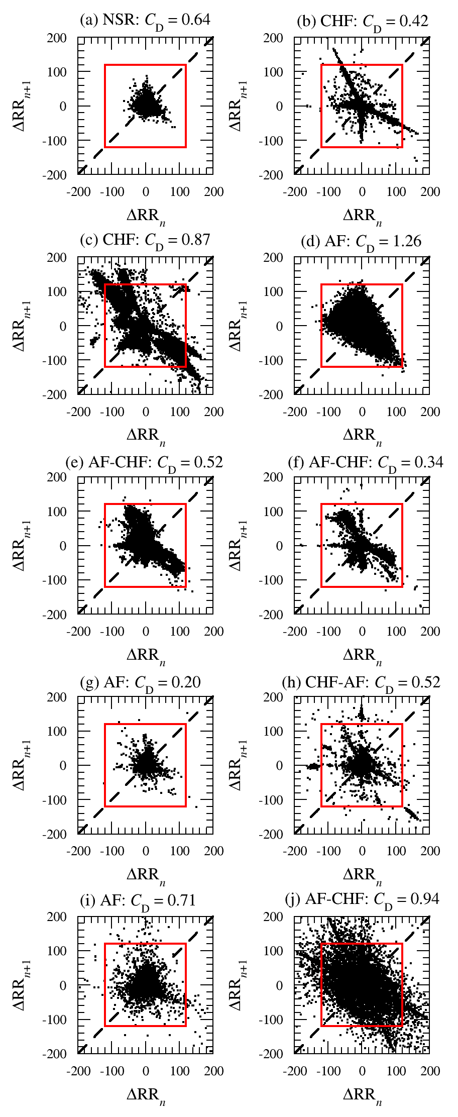
Figure 9: Examples of first-return maps built from the $\Delta$RR_n of patients diagnosed with normal sinus rhythm (a), congestive heart failure (b, c), atrial fibrillation (d, f), and preterm infants (g, j). While conditions reflected in (a f) are diagnosed cases, preterm infants were classified as AF and CHF-AF following our expertise.

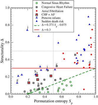
Figure 10: Permutation entropy $S_{\rm p}$ vs relative structurality $\Delta$ computed for cardiac dynamics data from various groups of patients. Each symbol corresponds to a given patient. See the legend to read the type of diagnosed cardiac dynamics. The equations of the continuous and dashed lines are also given in the legend. Symbols corresponding to the patients reported in Fig. 9 are here highlighted.

In Fig. 10 we present a general view of the analysis in the $S_{\rm p}$-$\Delta$ plane, where it can be observed how the different populations typically organize around specific areas. Healthy subjects are characterized by small structurality values bounded by $\Delta<0.375S_{\rm p}-0.075$ and $0.2<S_{\rm p}<0.7$, which is reflecting that a normal sinus rhythm is irregular due to the variability in the breathing rate and activity of the autonomic nervous system. However, abnormal rhythms like CHF and AF have also features clearly distinguishable with our dynamical complexity measure. Patients with CHF exhibit well marked segments in the RR sequence associated with ectopic beats characterized by $(S_{\rm p},\Delta)$ pairs above the straight line $\Delta>0.375S_{\rm p}-0.075$ and $S_{\rm p}<0.7$. AF induces relative structurality $\Delta>0.3$ and in most cases has an entropy $S_{\rm p}>0.6$ depending on how sustained is the AF. Some intermediate cases occur when patients present AF combined with ectopic beats. Finally, preterm infants distribute above the CHF patients but with slightly higher $\Delta$ values, while infants diagnosed with sudden death risk have, almost all of them, $S_{\rm p}>0.6$ and $\Delta>0.3$, compatible with an AF case, the exceptions corresponding to cases developing a mixture of CHF and AF or paroxysmal atrial fibrillation.

To assess the significance in the differences between the various groups of patients, we applied a $T$-test on the permutation entropy $S_{\rm p}$, the relative structurality $\Delta$, and the dynamical complexity $C_{\rm D}$, respectively. Results are reported in Tables 2 and 3. We retained five different groups of subjects for our statistical analysis: subjects with normal sinus rhythm (NSR), congestive heart failure (CHF), atrial fibrillation (AF), preterm newborns, and infants with sudden death risk (SDR). Permutation entropy $S_{\rm p}$ is significantly different among the five groups, but is not significantly different between NSR and CHF, as well as between SDR and AF (lower half of Table 2). The relative structurality $\Delta$ by itself allows to discriminate the five groups except preterm newborns from AF (upper half of Table 2). As a result of combining both markers, all the groups can be discriminated. Nevertheless, if the dynamical complexity is computed, it is not possible to distinguish NSF from CHF and preterm infants, CHF from preterm infants, and AF from SDR. These features result from some balance which can occur between the entropy $S_{\rm p}$ and the structurality $\Delta$. An accurate analysis is required in the $S_{\rm p}$-$\Delta$ plane to correctly characterize all the different groups.

Table 2: T-test to assess the significance in the difference of the permutation entropy $S_{\rm p}$ and the relative structurality $\Delta$ for the various groups of patients.

		NSR	CHF	AF	Preterm	SDR
	NSR	—	*	***	***	***	$\Delta$
	CHF	NS	—	***	**	***
	AF	***	***	—	NS	*
	Preterm	**	*	***	—	**
$S_{\rm p}$	SDR	***	***	NS	***	—
NSR $\equiv$ normal sinus rhythm, CHF $\equiv$ congestive heart failure, AF $\equiv$ atrial fibrillation, SDR $\equiv$ infant with sudden death risk, NS $\equiv$ Non-Significant, $*\equiv p<0.05$, $**\equiv p<5\cdot 10^{-3}$, $***\equiv p<5\cdot 10^{-4}$.

These results are partly recovered by using the sole dynamical complexity $C_{\rm D}$ as reported in Table 3. It clearly distinguishes NSR, CHF, and preterm from SDR and AF. These markers, whose computation cost is very reduced, allow therefore to correctly assess the complexity underlying the heart variability.

Table 3: $T$-test to assess the significance in the difference of the dynamical complexity $C_{\rm D}$ for the various groups of patients. Same terminology as described in the caption of Table 2.

		NSR	CHF	AF	Preterm	SDR
	NSR	—
	CHF	NS	—
	AF	***	***	—
	Preterm	NS	NS	***	—
	SDR	***	***	NS	***	—

V Conclusions

We have shown that to distinguish between organized and disorganized complexity, a marker capable of detecting a structured dynamics is needed independently of its degree of predictability. We propose a complexity measure combining these two notions of unpredictability, assessed with a permutation entropy, and that of structurality which quantifies, in a Poincaré section, how the structure underlying a dynamics can be described. The boundary conditions of our complexity measure are such that it vanishes for regular motion and whose upper limit reflects the disorganized dynamics of a stochastic signal, neither predictable nor easily describable in the Poincaré map. It thus provides a powerful measure for characterizing any stationary dynamics produced by either a map or a flow (as long as the time series can be investigated in a Poincaré plane), dissipative or conservative. It should be noted that our measure is not extensive and as such the upper limit can correspond to dynamics that can greatly differ in dimension. This problem can be addressed by using a Poincaré section whose dimension is greater than two but is out of the scope of the present work. As an illustration of its classifying power, we evidenced that this complexity measure can discriminate among various groups of common cardiac diseases from the sole measure of an ECG and we are confident that it will be useful for a reliable characterization of a large variety of real-world dynamics.

Appendix A Robustness of the dynamical complexity

In the following, we will provide an extensive analysis of the factors involved in the definition of the structurality $\Delta$ and how it behaves under the presence of different noise sources. The logistic map $x_{n}$ in Eq. (1) for $\mu=3.99$ was studied for different pixelation settings and lengths of the time series. In Fig. 11(left panel) we varied the number of boxes $N_{\rm b}^{2}$ in which is divided the renormalized frame of the first-return map for a time series of length $N_{\rm p}=10^{5}$. We observe (red curve) how the structurality converges to a very low value, as it should be for a well structured dynamics, when the number of boxes $N_{\rm b}>50$ (along one dimension). This points out to a possible parametrization of the number of boxes as a function of the number of points as $N_{\rm b}\sim 10\log_{10}N_{\rm p}$, as specified in the main text. This choice allows us to reduce the dependency of the results on the number of points $N_{\rm p}$ as it ensures that boxes are visited with a significant mean probability even when a small number of points ($N_{\rm p}<10^{4}$) is available. At the same time, the logarithmic dependence avoids the redundancy that could yield to underestimate $\Delta$. This is shown in the right column of the same Fig. 11, where both the permutation entropy $S_{\rm p}$ and the renormalized structurality $\Delta$ of the deterministic logistic map are almost independent of $N_{\rm p}$ when considering time series of lengths ranging from $N_{\rm p}=10^{3}$ up to $10^{5}$. Notice that the permutation entropy keeps a constant value when $N_{\rm p}>10^{4}$.

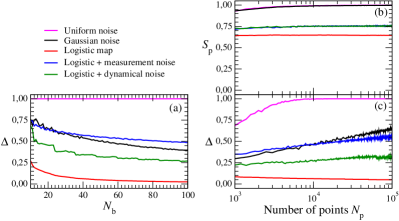
Figure 11: (a) Dependence of the renormalized structurality $\Delta$ on $N_{\rm b}$ (square root of the total number of boxes of the pixelation) for the deterministic logistic map for $\mu=3.99$ (red curve) and for the logistic map with Gaussian observational noise of standard deviation (std) $0.05$ ($B=0.2$) (blue curve), and with additive Gaussian dynamical noise of std $0.025$ ($B=0.1$) (green curve). As a reference, uniform noise (magenta) and Gaussian noise of std $0.25$ (black) are shown. In all cases, $N_{\rm p}=10^{5}$ are used. Dependence of the permutation entropy $S_{\rm p}$ (b) and structurality $\Delta$ (c) on the number of points $N_{\rm p}$ for the same cases indicated in the legend in the left panel. In all cases, $N_{\rm b}\sim 10\log_{10}N_{\rm p}$.

Regarding the effect of fluctuations present in the time series, we added a Gaussian noise $\xi_{n}$ (of zero mean and variance $0.0625$) to the deterministic time series simulating both observational ($q_{n}=x_{n}+B\xi_{n}$, blue curves) and dynamical ($x_{n+1}=\mu x_{n}(1-x_{n})+B\xi_{n}$, green curves) stochastic sources, with $B$ controlling the noise intensity. Again, Fig. 11 shows that the structurality obviously increases with respect to the pure deterministic case (red curve) but it is almost independent on the number of boxes as long $N_{\rm b}>50$. For comparison purposes, we also added the structurality of two pure stochastic processes, exhibiting intermediate values for the case of a Gaussian noise (black curve) and saturating at one for uniform noise (magenta curve) as it should be since the uniform noise is uniformly distributed in the renormalized frame. Looking at the right column of Fig. 11, it is worth noting how the structurality is able to distinguish the logistic map with added observational and dynamical noises (blue and green curves) while the permutation entropy is not. Another remark is that while the permutation entropy is maximum for both uniform and Gaussian noise (they have the same degree of unpredictability), the structurality (right column-bottom panel) only saturates for the uniform noise and linearly increases with the number of points in the case of the Gaussian noise. A final observation in this study, it is that it is safe to consider for both $S_{\rm p}$ and $\Delta$, $N_{\rm p}>10^{4}$, in agreement with what was already obtained with a Shannon entropy computed from recurrence plots Letellier (2006).

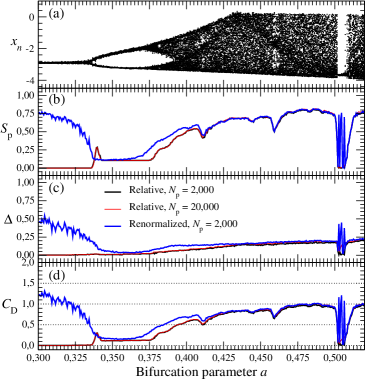
Figure 12: Dynamics of the Rössler system with added Gaussian dynamical noise of std $0.005$ ($B=0.02$) for varying bifurcation parameter $a$. (a) Bifurcation diagram, (b) permutation entropy $S_{\rm p}$, (c) structurality $\Delta$, and (d) dynamical complexity $C_{\rm D}$. From (b) to (c), each curve denotes the corresponding marker computed using relative ($N_{\rm p}=2,000$ in black and $N_{\rm p}=20,000$ in red) and renormalized frames ($N_{\rm p}=2,000$ in blue). Other parameter values: $b=2$ and $c=4$.

Another factor affecting our structurality measure is the framing of the Poincaré section. To show how the choice of a renormalized or relative frame is actually contributing to $\Delta$, we computed the bifurcation diagram of the Rössler system with the parameter $a$ [Eq. 9 with $\rho_{z}=0$ and $a_{1}=a$] and influenced by a Gaussian dynamical noise of zero mean and standard deviation $0.005$. Since the noise contamination is quite limited, the dynamical complexity is mainly driven by the permutation entropy while the relative structurality (red traces in both panels) slightly increases with the parameter $a$: the more the chaos develops, the thicker the first-return map and the larger the relative structurality. However, when considering a renormalized frame, huge discrepancies are clear between the two frames in the period-one windows. A renormalized frame is no longer able to correctly detect the deterministic part of the dynamics and over estimates the noise contribution. For instance the entropy as well as the structurality are arbitrarily large for $a<0.33$ and there is a large instability in the period-1 window at $0.502<a<0.508$. In these period-1 windows, a relative frame provides more stable results with the three markers, $S_{\rm p}$, $\Delta$ and $C_{\rm D}$ exhibiting low values despite the noise contamination.

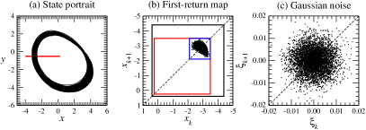
Figure 13: Dependence of the complexity markers on the chosen reference frame. (a) State portrait of a noisy period-one limit cycle produced by one of the Rössler systems (9) with a Gaussian dynamical noise of standard deviation $0.00375$. The center of the limit cycle is at $(0.25,-0.25)$ and the red line extending from $x=-3.46$ to $x=0.25$ is the projection of a Poincaré plane. (b) First-return map of the Poincaré section of (a) framed by the renormalized frame (blue square), and the relative frames of the largest chaotic attractor in the bifurcation diagram shown in Fig. 12(a) (black square) and of the period-one limit cycle (red square). (c) First-return map of the Gaussian noise injected in (a) and plotted in the renormalized frame.

The overestimation of the noise contribution to a period-one limit cycle is further illustrated in Fig. 13. The Poincaré plane is plotted as a red line in the state portrait of Fig. 13(a). The size of the corresponding Poincaré section (the crossings of the limit cycle with the Poincaré plane) defines the renormalized frame ($-3.4<x_{n}<-2.15$) shown as a blue square in Fig. 13(b). It is clear that the period-one limit cycle no longer appears as a structured dynamics with respect to the renormalized frame due to the noise contamination. However, when observing the Poincaré section using a relative frame as the one defined by the size of the largest chaotic attractor of the bifurcation diagram (black square) or by the period-one limit cycle (red square), the noise contribution to the structurality is damped and the dynamics reveals to be more structured. Just to compare, the first-return map of the Gaussian noise injected in the limit cycle is shown in Fig. 13(c) in a renormalized frame. The values of the three complexity markers for each one of the three frames shown in Fig. 13(b) are reported in Table 4. There it is clear the relevance of the frame definition, showing a significant difference between choosing a relative or a renormalized frame.

Finally, note that to avoid overestimating the entropy, permutations are performed only when $|x_{i}-x_{i+1}|>\epsilon$ with $\epsilon=5l_{\rm b}$. This kind of noise filter is in fact related to uncertainties inherent to measurements and allows to reduce the typical peaks appearing at the bifurcations in a period doubling cascade when observational noise is affecting the dynamical system (see Fig. 2e in Ref. Bandt and Pompe (2002)) or avoids to have large entropy in the case of a noisy period-one limit cycle (Fig. 12).

Table 4: Values of the complexity markers $S_{\rm p}$, $\Delta$, and $C_{\rm D}$ for the the noisy period-one limit cycle shown using the three different frames marked in Fig. 13(b).

Frame	$S_{\rm p}$	$\Delta$	$C_{\rm D}$
Relative (largest attractor)	0.06	0.04	0.10
Relative (limit cycle radius)	0.16	0.07	0.23
Renormalized	0.70	0.44	1.14

References

- Adami et al. (2000) C. Adami, C. Ofria, and T. C. Collier, Proceedings of the National Academy of Sciences 97, 4463 (2000).
- Perkiömäki et al. (2005) J. S. Perkiömäki, T. H. Mäkikallio, and H. V. Huikuri, Clinical and Experimental Hypertension 27, 149 (2005).
- Regev (2006) O. Regev, Chaos and Complexity in Astrophysics (Cambridge University Press, 2006).
- Sabeti et al. (2009) M. Sabeti, S. Katebi, and R. Boostani, Artificial Intelligence in Medicine 47, 263 (2009).
- Flack and Krakauer (2011) J. C. Flack and D. C. Krakauer, Chaos 21, 037108 (2011).
- Aquino et al. (2017) A. L. Aquino, H. S. Ramos, A. C. Frery, L. P. Viana, T. S. Cavalcante, and O. A. Rosso, Physica A 465, 277 (2017).
- Pozo et al. (2017) J. M. Pozo, A. J. Geers, M.-C. Villa-Uriol, and A. F. Frangi, Journal of Fluid Mechanics 825, 704 (2017).
- Lloyd (2001) S. Lloyd, IEEE Control Systems Magazine 21, 7 (2001).
- Kolmogorov (1958) A. N. Kolmogorov, Doklady Akademii Nauk SSSR 119, 861 (1958).
- Sinai (1959) G. Sinai, Doklady Akademii Nauk SSSR 124, 768 (1959).
- Shannon (1948) C. E. Shannon, Bell System Technical Journal 27, 379 (1948).
- Jaynes (1957) E. T. Jaynes, Physical Review 106, 620 (1957).
- Skilling and Bryan (1984) J. Skilling and R. K. Bryan, Monthly Notices of the Royal Astronomical Society 211, 111 (1984).
- Berger et al. (1996) A. L. Berger, S. A. D. Pietra, and V. J. D. Pietra, Computational Linguistics 22, 39 (1996).
- Larivee and Brown (1992) R. J. Larivee and S. D. Brown, Analytical Chemistry 64, 2057 (1992).
- Fresnel et al. (2015) E. Fresnel, E. Yacoub, U. Freitas, A. Kerfourn, V. Messager, E. Mallet, J.-F. Muir, and C. Letellier, Chaos 25, 083111 (2015).
- Weaver (1948) W. Weaver, American Scientist 36, 536 (1948).
- Huberman and Hogg (1986) B. A. Huberman and T. Hogg, Physica D 22, 376 (1986).
- Feldman and Crutchfield (1998) D. P. Feldman and J. P. Crutchfield, Physics Letters A 238, 244 (1998).
- Crutchfield and Young (1989) J. P. Crutchfield and K. Young, Physical Review Letters 63, 105 (1989).
- R. López-Ruiz and Calbet (1995) H. L. M. R. López-Ruiz and X. Calbet, Physics Letters A 209, 321 (1995).
- Martin et al. (2003) M. T. Martin, A. Plastino, and O. A. Rosso, Physics Letters A 311, 126 (2003).
- Letellier (2008) C. Letellier, Chaos, Solitons & Fractals 36, 32 (2008).
- Letellier (2006) C. Letellier, Physical Review Letters 96, 254102 (2006).
- Bandt and Pompe (2002) C. Bandt and B. Pompe, Physical Review Letters 88, 174102 (2002).
- Charó et al. (2019) G. D. Charó, D. Sciamarella, S. Mangiarotti, G. Artana, and C. Letellier, Chaos 29, 123126 (2019).
- Rössler and Ortoleva (1978) O. E. Rössler and P. J. Ortoleva, Lecture Notes in Biomathematics 21, 67 (1978).
- Farmer (1982) J. D. Farmer, Physica D 4, 366 (1982).
- Hénon and Heiles (1964) M. Hénon and C. Heiles, The astronomical Journal 69, 73 (1964).
- Lichtenberg and Lieberman (1992) A. Lichtenberg and M. Lieberman, Regular and chaotic dynamics, Applied Mathematical Sciences, Vol. 38 (Springer-Verlag, 1992).
- Couliette and Wiggins (2000) C. Couliette and S. Wiggins, Nonlinear Processes in Geophysics 7, 59 (2000).
- Shadden et al. (2005) S. C. Shadden, F. Lekien, and J. E. Marsden, Physica D 212, 271 (2005).
- Boccaletti et al. (2006) S. Boccaletti, V. Latora, Y. Moreno, M. Chavez, and D.-U. Hwang, Physics Reports 424, 175 (2006).
- Sendiña-Nadal et al. (2016) I. Sendiña-Nadal, S. Boccaletti, and C. Letellier, Physical Review E 94, 042205 (2016).
- Mackey and Glass (1977) M. C. Mackey and L. Glass, Science 197, 287 (1977).
- Letellier et al. (1995) C. Letellier, L. L. Sceller, P. Dutertre, G. Gouesbet, Z. Fei, and J. L. Hudson, Journal of Physical Chemistry 99, 7016 (1995).
- Letellier et al. (2018) C. Letellier, S. Mangiarotti, I. Sendiña-Nadal, and O. E. Rössler, Chaos 28, 045107 (2018).
- Dutertre (1995) P. Dutertre, Caractérisation des attracteurs étranges par la population d’orbites périodiques, Ph.D. thesis, Université de Rouen, France (1995).
- Wang and Hudson (1991) Y. Wang and J. L. Hudson, AIChE Journal 37, 1833 (1991).
- Goldberger et al. (2000) A. L. Goldberger, L. A. N. Amaral, L. Glass, J. M. Hausdorff, P. C. H. Ivanov, R. G. Mark, J. E. Mietus, G. B. Moody, C.-K. Peng, and H. E. Stanley, Circulation 101, e215 (2000).
- Allessie et al. (1996) M. A. Allessie, K. Konings, C. J. Kirchhof, and M. Wijffels, American Journal of Cardiology 77, 10A (1996).
- Goldstein and Barnett (1967) R. E. Goldstein and G. O. Barnett, Computers and Biomedical Research 1, 146 (1967).
- Meijler et al. (1968) F. L. Meijler, J. Strackee, F. J. L. van Cappelle, and J. C. du Perron, Circulation Research 22, 695 (1968).
- Bootsma et al. (1970) B. K. Bootsma, A. J. Hoelen, J. Strackee, and F. L. Meijler, Circulation 41, 783 (1970).
- Baim et al. (1986) D. S. Baim, W. S. Colucci, E. S. Monrad, H. S. Smith, R. F. Wright, A. Lanoue, D. F. Gauthier, B. J. Ransil, W. Grossman, and E. Braunwald, it Journal of the American College of Cardiology 7, 661 (1986).
- Burstein and Nattel (2008) B. Burstein and S. Nattel, Journal of the American College of Cardiology 51, 802 (2008).
- Pellman and Sheikh (2015) J. Pellman and F. Sheikh, Comprehensive Physiology 5, 649 (2015).
- Gee et al. (2017) A. H. Gee, R. Barbieri, D. Paydarfar, and P. Indic, IEEE Transactions on Biomedical Engineering 64, 2300 (2017).
- Yacoub (2011) E. Yacoub, Suivi cardio-respiratoire des nourrissons à risque, Ph.D. thesis, Normandie University, Rouen, France (2011).
- Camm et al. (2012) A. J. Camm, S. M. Al-Khatib, H. Calkins, J. L. Halperin, P. Kirchhof, G. Y. Lip, S. Nattel, J. Ruskin, A. Banerjee, D. Blendea, E. Guasch, M. Needleman, I. Savelieva, J. Viles-Gonzalez, and E. S. Williams, American Heart Journal 164, 292 (2012).