NPSA: Nonorthogonal Principal Skewness Analysis

Abstract

Principal skewness analysis (PSA) has been introduced for feature extraction in hyperspectral imagery. As a third-order generalization of principal component analysis (PCA), its solution of searching for the locally maximum skewness direction is transformed into the problem of calculating the eigenpairs (the eigenvalues and the corresponding eigenvectors) of a coskewness tensor. By combining a fixed-point method with an orthogonal constraint, it can prevent the new eigenpairs from converging to the same maxima that has been determined before. However, the eigenvectors of the supersymmetric tensor are not inherently orthogonal in general, which implies that the results obtained by the search strategy used in PSA may unavoidably deviate from the actual eigenpairs. In this paper, we propose a new nonorthogonal search strategy to solve this problem and the new algorithm is named nonorthogonal principal skewness analysis (NPSA). The contribution of NPSA lies in the finding that the search space of the eigenvector to be determined can be enlarged by using the orthogonal complement of the Kronecker product of the previous one, instead of its orthogonal complement space. We give a detailed theoretical proof to illustrate why the new strategy can result in the more accurate eigenpairs. In addition, after some algebraic derivations, the complexity of the presented algorithm is also greatly reduced. Experiments with both simulated data and real multi/hyperspectral imagery demonstrate its validity in feature extraction.

I Introduction

SINCE hyperspectral imagery consists of tens or hundreds of bands with a very high spectral resolution, it has drawn more attention from various applications in the past decades, such as spectral unmixing[1, 2], classification[3, 4], target detection[5, 6] and so on. However, high spectral dimensionality with strong intraband correlations also results in informantion redundancy and computational burden of data processing[7].Therefore, dimensionality reduction (DR) has become one of the most important techniques for addressing these problems. DR can be categorized into two classes: feature extraction and feature selection. In this paper, we mainly focus on the former.

The most commonly used feature extraction algorithm is principal component analysis (PCA)[8], which aims to search for the projection direction that maximizes the variance. Its solution corresponds to the eigenvectors of the image’s covariance matrix. Several techniques that originated from PCA have been developed, such as kernel PCA (KPCA)[9] and maximum noise fraction (MNF)[10]. KPCA is a nonlinear extension of PCA, which transforms the data into a higher dimensional space via a mapping function and then performs the PCA method. MNF is another popular method for feature extraction, which considers the image quality and selects the signal-to-noise ratio (SNR) as the measure index.

The methods mentioned above mainly focus on the second-order statistical characteristics of the data. However, the distribution of many real data sets usually does not satisfy the Gaussian distribution. Therefore, these methods may have a poor performance and cannot reveal the intrinsical structure of the data. In this case, many methods based on the higher-order statistics have been paid more attention in recent years and have been applied in many remote sensing fields, including anomaly detection[11, 12], endmember extraction[13], target detection[14, 15]. Independent component analysis (ICA) is one of the most successful feature extraction techniques. It was derived from the blind source separation (BSS) application, which attempts to find a linear representation of non-Gaussian data so that the components are statistically independent, or as independent as possible[16]. Several widely-used algorithms include joint approximate diagonalization of eigen-matrices (JADE)[17] and Fast Independent Component Analysis (FastICA)[18]. JADE utilizes the fourth-order culumant tensor of the data. Some algorithms that originated from JADE have been developed later. A third-order analogue called Skewness-based ICA via Eigenvectors of Cumulant Operator (EcoICA) is proposed[19]. Other joint diagonalization methods include subspace fitting method (SSF)[20], Distinctively Normalized Joint Diagonalization (DNJD)[21] and Alternating Columns-Diagonal Centers (ACDC)[22], etc.

FastICA can select skewness, negentropy or other indices as the non-Gaussian measurement. It can reach a cubic convergence rate and outperform most of the other commonly used ICA algorithms[23]. However, it requires all the pixels to be involved in each iteration for searching for the optimal projection direction, which is quite time-consuming, especially for the high dimensional data. To solve this problem, Geng et al. has proposed an efficient method called Principal Skewness Analysis (PSA)[24]. PSA can be viewed as a third-order generalization of PCA. Meanwhile, it is also equivalent to FastICA when selecting the skewness as a non-Gaussian index. Following this work, a momentum version (called MPSA) to alliviate the oscillation phenomenon of PSA [25] and a natural fourth-order extension method, i.e., Principal Kurtosis Analysis (PKA)[26] are also analyzed.

The solution of these PSA-derived methods can be transformed into the problem of calculating the eigenvalues and the corresponding eigenvectors of the tensor, which is similar to PCA. By adopting the fixed-point scheme, the solution can be obtained iteratively. To prevent the solution from converging to the same one that has been determined previously, an orthogonal complement operator is also introduced in these methods. Thus all of them can obtain an orthogonal transformation matrix eventually, since the search space of the eigenvector to be determined is always restricted in the orthogonal complement space of the previous one. However, theoretical analysis based on multi-linear algebra has shown that the eigenvectors of a supersymmetric tensor are not inherently orthogonal in general [27, 28], which is different from the situation for the real symmetric matrix. Thus the orthogonal constraint in PSA and the inherent nonorthogonality of the eigenvectors of supersymmetric tensor are a pair of irreconcilable contradictions. In this paper, we propose a more relaxed constraint, and based on this, a new algorithm, which is named nonorthogonal principal skewness analysis (NPSA), is presented to deal with this problem. It is expected that NPSA can have the following two attributes: 1) similar to PSA, it can also prevent the eigenvector to be determined from converging to the eigenvectors that have been determined previously; 2) it can obtain a more accurate solution than that of PSA meanwhile.

The rest of this paper is organized as follows. In Section II, we briefly review the original PSA algorithm and analyze its deficiencies with a simple example. In Section III, we present the new strategy in NPSA first and then obtain an improved version when taking the complexity into consideration. Two strategies are compared in the end of this section. In Section IV, we give some theoretical analysis to justify the validity of the algorithm. Some experimental results are given in Section V, and the conclusions are drawn in Section VI.

II Background

In this section, we first introduce some notations, basic definitions and important properties used throughout this paper, and then give a brief review of the formations and deficiencies of PSA.

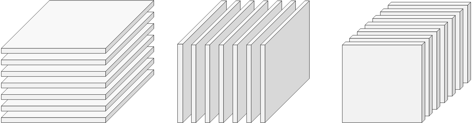
Figure 1:  Slices of a third-order tensor, i.e., horizontal slices $\mathbf{A}_{i::}$, lateral slices $\mathbf{A}_{:j:}$ and frontal slices $\mathbf{A}_{::k}$.

II-A Preliminaries

Following [29], in this paper, the high-order tensors are denoted by boldface Euler script letters, e.g., $\mathcal{A}$. A $N$th-order tensor is defined as $\mathcal{A}\in R^{I_{1}\times I_{2}\times\dots\times I_{N}}$, where $N$ is the order of $\mathcal{A}$, also called the way or mode. For $N$=$1$, it is a vector. For $N$=$2$, it is a matrix. The element of $\mathcal{A}$ is denoted by $a_{i_{1},i_{2},\dots,i_{N}},i_{n}\in\{{1,2,\dots,I_{n}}\},1\leq n\leq N$. Fibers, the higher-order analogue of matrix rows and columns, are defined by fixing every index except for one. Slices are two-dimensional sections of a tensor, defined by fixing all except for two indices. For a third-order tensor $\mathcal{A}\in R^{I_{1}\times I_{2}\times I_{3}}$, as shown in Fig. 1, its three different slices are called horizontal, lateral and frontal slices, which can be denoted by $\mathbf{A}_{i::},\mathbf{A}_{:j:},\mathbf{A}_{::k}$, respectively. Compactly, the $k$th frontal slice is also denoted as $\mathbf{A}_{k}$. A tensor is called supersymmetric if its elements remain invariant under any permutation of the indices[29].

Some important operations are illustrated as follows: $\circ$ denotes the outer product of two vectors. The operator $\rm vec$ is to reorder the elements of a matrix or a higher-order tensor into a vector and $\rm unvec$ is the opposite. The $n$-mode product of a tensor $\mathcal{A}\in R^{I_{1}\times I_{2}\dots\times I_{N}}$ with a matrix $\mathbf{U}\in R^{J\times I_{n}}$ is denoted by $\mathcal{A}\times_{n}\mathbf{U}\in R^{I_{1}\times\dots\times I_{n-1}\times J\times I_{n+1}\times\dots\times I_{N}}$, whose element is $(\mathcal{A}\times_{n}\mathbf{U})_{i_{1}\dots i_{n-1}ji_{n+1}\dots i_{N}}=\sum_{i_{n}=1}^{I_{n}}a_{i_{1},i_{2},\dots,i_{N}}u_{ji_{n}}$. The range of a matrix $\mathbf{A}\in R^{m\times n}$ is defined as $\rm R(\mathbf{A})=\{\mathbf{y}\in\it{R}^{m}|\mathbf{A}\mathbf{x}=\mathbf{y},\mathbf{x}\in\it{R}^{n}\}$ and its dimensionality is denoted by $\rm dim[\rm R(\mathbf{A})]$. $N^{+}$ denotes the set of all positive integers.

The Kronecker product of two matrices $\mathbf{A}\in R^{I\times J}$ and $\mathbf{B}\in R^{K\times L}$ is a matrix denoted as $\mathbf{A}\otimes\mathbf{B}\in R^{IK\times JL}$, which is defined as

$$\begin{split}\mathbf{A}\otimes\mathbf{B}&=\begin{bmatrix}a_{11}\mathbf{B}&\dots&a_{1J}\mathbf{B}\\ &\ddots&\vdots\\ a_{I1}\mathbf{B}&\dots&a_{IJ}\mathbf{B}\end{bmatrix}\end{split}.$$ (1)

For simplicity, we use $\mathbf{A}^{\otimes^{p}}$ and $\mathbf{a}^{\otimes^{p}}$ to denote the $p$-times Kronecker Product of the matrix $\mathbf{A}$ and the vector $\mathbf{a}$, respectively.

The properties that will be used later are presented here[30, 31],

$$(\mathbf{A}\otimes\mathbf{B})^{\mathrm{T}}=\mathbf{A}^{\mathrm{T}}\otimes\mathbf{B}^{\mathrm{T}},$$ (2)

$$(\mathbf{A}\otimes\mathbf{B})^{\mathrm{-1}}=\mathbf{A}^{\mathrm{-1}}\otimes\mathbf{B}^{\mathrm{-1}},$$ (3)

$$(\mathbf{A}\otimes\mathbf{C})(\mathbf{B}\otimes\mathbf{D})=(\mathbf{A}\mathbf{B})\otimes(\mathbf{C}\mathbf{D}),$$ (4)

$$\rm rank(\mathbf{A}\otimes\mathbf{B})=\rm rank(\mathbf{A})\rm rank(\mathbf{B}),$$ (5)

$$\rm vec(\mathbf{A}+\mathbf{B})=\rm vec(\mathbf{A})+\rm vec(\mathbf{B}),$$ (6)

$$\rm vec(\mathbf{A}\mathbf{B}\mathbf{C})=(\mathbf{C}^{\mathrm{T}}\otimes\mathbf{A})\rm vec(\mathbf{B}),$$ (7)

$$\begin{split}\rm vec(\mathcal{S}\times_{1}\mathbf{A}^{(1)}\times_{2}\mathbf{A}^{(2)}\dots\times_{n}\mathbf{A}^{(n)})=\\ (\mathbf{A}^{(n)}\otimes\mathbf{A}^{(n-1)}\otimes\dots\otimes\mathbf{A}^{(1)})^{\mathrm{T}}\rm vec(\mathcal{S}).\end{split}$$ (8)

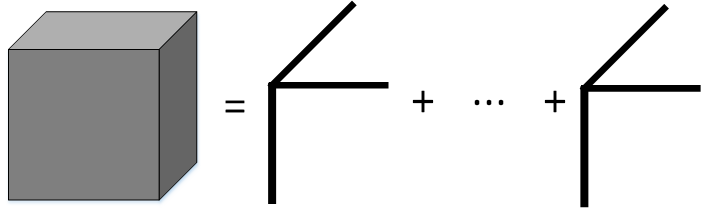
Figure 2:  Sktech map of the calculation of the coskewness tensor $\mathcal{S}$.

II-B PSA Algortithm

In PSA, the coskewness tensor, the analogue of the covariance matrix in PCA, is constructed to calculate the skewness of the image in the direction $\mathbf{u}$.

Assuming that the image data set is $\mathbf{X}=[\mathbf{x}_{1},\mathbf{x}_{2},\dots,\mathbf{x}_{N}]\in R^{L\times N}$, where $\mathbf{x}_{i}$ is the $L\times 1$ vector and $N$ is the number of pixels. The image should first be centralized and whitened by

$$\mathbf{R}=\mathbf{F}^{\mathrm{T}}(\mathbf{X}-\mathbf{m}),$$ (9)

where $\mathbf{m}=(1/N)\sum_{i=1}^{N}\mathbf{x}_{i}$ is the mean vector and $\mathbf{R}=[\mathbf{r}_{1},\mathbf{r}_{2},\dots,\mathbf{r}_{N}]$ is the whitened image. $\mathbf{F}=\mathbf{E}\mathbf{D}^{-\frac{1}{2}}$ is called the whitening operator, where $\mathbf{E}$ represents the eigenvector matrix of the covariance matrix and $\mathbf{D}$ is the corresponding eigenvalue diagonal matrix.

Then, the coskewness tensor is calculated by

$$\mathcal{S}=\frac{1}{N}\sum\limits_{i=1}^{N}\mathbf{r}_{i}\circ\mathbf{r}_{i}\circ\mathbf{r}_{i}.$$ (10)

Fig. 2 shows a sketch map of the calculation of $\mathcal{S}$. Obviously, $\mathcal{S}$ is a supersymmetric tensor with a size of $L\times L\times L$.

Then the skewness of an image in any direction $\mathbf{u}$ can be calculated by

$$\rm skew(\mathbf{u})=\mathcal{S}\times_{1}\mathbf{u}\times_{2}\mathbf{u}\times_{3}\mathbf{u},$$ (11)

where $\mathbf{u}\in R^{L\times 1}$ is a unit vector, i.e., $\mathbf{u}^{\mathrm{T}}\mathbf{u}=1$.

So the optimization model can be formulated as

$$\begin{cases}\max\limits_{\mathbf{u}}\mathcal{S}\times_{1}\mathbf{u}\times_{2}\mathbf{u}\times_{3}\mathbf{u}\\ s.t.\mathbf{u}^{\mathrm{T}}\mathbf{u}=1\end{cases}.$$ (12)

Using the Lagrangian method, the problem is equivalent to solving the equation

$$\mathcal{S}\times_{1}\mathbf{u}\times_{3}\mathbf{u}=\lambda\mathbf{u}.$$ (13)

A fixed-point method is performed to calculate $\mathbf{u}$ for each unit, which can be expressed as follows:

$$\begin{cases}\mathbf{u}=\mathcal{S}\times_{1}\mathbf{u}\times_{3}\mathbf{u}\\ \mathbf{u}=\mathbf{u}/\|\mathbf{u}\|_{2}\end{cases}.$$ (14)

If it does have a fixed-point, the solution $\mathbf{u}$ is called the first principal skewness direction and $\lambda$ is the skewness of the image in the direction $\mathbf{u}$. Equivalently, $(\lambda,\mathbf{u})$ is also called the eigenvalue/eigenvector pair of a tensor, introduced by Lim [32] and Qi[33].

To prevent the second eigenvector from converging to the same one as the first, the algorithm projects the data into the orthogonal complement space of $\mathbf{u}$, which is equivalent to generate a new tensor by calculating the $n$-mode product

$$\mathcal{S}=\mathcal{S}\times_{1}\mathbf{P}_{\mathbf{u}}^{\bot}\times_{2}\mathbf{P}_{\mathbf{u}}^{\bot}\times_{3}\mathbf{P}_{\mathbf{u}}^{\bot},$$ (15)

where $\mathbf{P}_{\mathbf{u}}^{\bot}=\mathbf{I}-\mathbf{u}(\mathbf{u}^{\mathrm{T}}\mathbf{u})^{-1}\mathbf{u}^{\mathrm{T}}$ is the orthogonal complement projection operator of $\mathbf{u}$ and $\mathbf{I}$ is the $L\times L$ identity matrix.

Then, the same iteration method, i.e., (14), can be applied to the new tensor $\mathcal{S}$ to obtain the second eigenvector and the following process is conducted in the same manner.

II-C Deficiencies Of PSA

As mentioned before, an orthogonal complement operator is introduced in PSA in order to prevent the next eigenvector from converging to the eigenvectors that have been determined previously. As is well known, the eigenvectors of a real symmetric matrix is naturally orthogonal to each other. However, this may not hold when generalized to the higher-order cases.

We here present a simple example to illustrate this phenomenon. Consider a supersymmetric tensor $\mathcal{S}\in R^{2\times 2\times 2}$, whose two frontal slices are

$$\begin{split}\mathbf{S}_{1}=\begin{bmatrix}2&-1\\ -1&0.8\end{bmatrix},\mathbf{S}_{2}=\begin{bmatrix}-1&0.8\\ 0.8&0.3\end{bmatrix}\end{split}.$$

It can easily verifed that its two eigenvectors are

$$\mathbf{u}_{1}=[0.8812,-0.4727]^{\mathrm{T}},\mathbf{u}_{2}=[0.3757,0.9267]^{\mathrm{T}},$$

and their inner product is $\mathbf{u}_{1}^{\mathrm{T}}\mathbf{u}_{2}=-0.1070$, which means that they are nonorthogonal. However, the results obtained by the PSA algorithm are

$$\mathbf{u}_{1}^{\rm PSA}=[0.8812,-0.4727]^{\mathrm{T}},\mathbf{u}_{2}^{\rm PSA}=[0.4727,0.8812]^{\mathrm{T}},$$

which are orthogonal. It is apparent that $\mathbf{u}_{2}^{\rm PSA}$ deviates from $\mathbf{u}_{2}$, and they have a $6.1430^{\circ}$ angle. The error is caused by the orthogonal constraint used in PSA. Therefore, how to obtain the more accurate eigenpairs is significant.

III NPSA

III-A New Search Strategy

Here, we first give the new search strategy in NPSA and then theoretically illustrate why this method can obtain the more accurate eigenpairs in the next section.

Similar to PSA, the first eigenvector $\mathbf{u}$ can be obtained according to (14). The subsequent steps are presented as follows:

(1): vectorize the tensor $\mathcal{S}$ into a vector $\mathbf{s}$. Usually, The vectorization of a third-order tensor is defined as the vertical arrangement of column vectorization of the front-slice matrix [31], i.e., $\mathbf{s}=\rm vec(\mathcal{S})=[\mathbf{s}_{1}^{\mathrm{T}},\mathbf{s}_{2}^{\mathrm{T}},\dots,\mathbf{s}_{\it L}^{\mathrm{T}}]^{\mathrm{T}}$ $\in$ $R^{L^{3}\times 1}$, where $\mathbf{s}_{i}\in R^{L^{2}\times 1}$ is the vector generated by the $i$-th frontal slice $\mathbf{S}_{i}$ , i.e., $\mathbf{s}_{i}=\rm vec(\mathbf{S}_{i})$ .

(2): compute a new vector via the $3$-times Kronecker product of the vector $\mathbf{u}$, denoted by $\mathbf{u}^{\otimes^{3}}=\mathbf{u}\otimes\mathbf{u}\otimes\mathbf{u}$ .

(3): compute the orthogonal complement projection matrix of $\mathbf{u}^{\otimes^{3}}$, which can be expressed as

$$\mathbf{P}^{\bot}_{\mathbf{u}^{\otimes^{3}}}=\mathbf{I}^{\otimes^{3}}-\mathbf{u}^{\otimes^{3}}[(\mathbf{u}^{\otimes^{3}})^{\mathrm{T}}\mathbf{u}^{\otimes^{3}}]^{-1}(\mathbf{u}^{\otimes^{3}})^{\mathrm{T}},$$ (16)

where $\mathbf{I}^{\otimes^{3}}$ is the 3-times Kronecker product of the matrix $\mathbf{I}$ of (15) and it is a $L^{3}\times L^{3}$ identity matrix.

(4): multiply $\mathbf{P}^{\bot}_{\mathbf{u}^{\otimes^{3}}}$ and the vectorized tensor $\mathbf{s}$ in step (1) and then perform the $\rm unvec$ operation to obtain a new tensor. Without causing ambiguity and to have a concise form, we still express the updated tensor as $\mathcal{S}$. Thus we can have

$$\mathcal{S}=\rm unvec(\mathbf{P}^{\bot}_{\mathbf{u}^{\otimes^{3}}}\cdot\mathbf{s}).$$ (17)

Then we can obtain the second eigenvector by performing the fixed-point scheme, i.e., (14), to the new updated tensor and similarly repeat the above process until we get all or pre-set eigenpairs.

For the example mentioned in the previous section, the two eigenvectors obtained by NPSA are

$$\mathbf{u}_{1}^{\rm NPSA}=[0.8812,-0.4727]^{\mathrm{T}},\mathbf{u}_{2}^{\rm NPSA}=[0.3351,0.9422]^{\mathrm{T}}.$$

The angle between $\mathbf{u}_{2}^{\rm NPSA}$ and $\mathbf{u}_{2}$ is $2.4874^{\circ}$, which is less than that between $\mathbf{u}_{2}^{\rm PSA}$ and $\mathbf{u}_{2}$, as shown in Fig. 3. It means that the new search strategy presented in NPSA is actually efficient.

Figure 3: The distribution of the true eigenvectors, and those obtained by NPSA and PSA in an unit circle.

III-B Complexity Reduction

In this subsection, we take the complexity into consideration. It can be observed that although the strategy shown in step (1) $\sim$ step (4) is efficient, there are still some problems in the implementation: 1) it needs to perform the $\rm vec$ and $\rm unvec$ operations repeatedly; 2) computing the orthogonal projection matrix $\mathbf{P}^{\bot}_{\mathbf{u}^{\otimes^{3}}}$ takes up an $L^{3}\times L^{3}$ memory. When $L$ becomes larger, especially for hyperspectral images with tens or hundreds of bands, the computational burden is huge and unbearable. So in the following, we try to reduce the computational complexity and to save the storage memory simultaneously.

For (16), based on (2) and (4), we can derive

$$\begin{split}(\mathbf{u}^{\otimes^{3}})^{\mathrm{T}}\mathbf{u}^{\otimes^{3}}&=(\mathbf{u}\otimes\mathbf{u}\otimes\mathbf{u})^{\mathrm{T}}(\mathbf{u}\otimes\mathbf{u}\otimes\mathbf{u})\\ &=(\mathbf{u}^{\mathrm{T}}\mathbf{u})\otimes(\mathbf{u}^{\mathrm{T}}\mathbf{u})\otimes(\mathbf{u}^{\mathrm{T}}\mathbf{u})\\ &=1.\end{split}$$ (18)

It means that the vector generated by the $3$-times Kronecker product of a unit vector is still with a unit length. In this way, (16) can be simplified as

$$\begin{split}\mathbf{P}^{\bot}_{\mathbf{u}^{\otimes^{3}}}&=\mathbf{I}^{\otimes^{3}}-\mathbf{u}^{\otimes^{3}}(\mathbf{u}^{\otimes^{3}})^{\mathrm{T}}\\ &=\mathbf{I}^{\otimes^{3}}-(\mathbf{u}\mathbf{u}^{\mathrm{T}})\otimes(\mathbf{u}\mathbf{u}^{\mathrm{T}})\otimes(\mathbf{u}\mathbf{u}^{\mathrm{T}}).\end{split}$$ (19)

According to (17), the new tensor $\mathcal{S}$ can be updated by

$$\begin{split}\mathcal{S}&=\rm unvec(\mathbf{P}^{\bot}_{\mathbf{u}^{\otimes^{3}}}\cdot\mathbf{s})\\ &=\rm unvec([\mathbf{I}^{\otimes^{3}}-(\mathbf{u}\mathbf{u}^{\mathrm{T}})\otimes(\mathbf{u}\mathbf{u}^{\mathrm{T}})\otimes(\mathbf{u}\mathbf{u}^{\mathrm{T}})]\cdot\mathbf{s})\\ &=\mathcal{S}-\rm unvec[((\mathbf{u}\mathbf{u}^{\mathrm{T}})\otimes(\mathbf{u}\mathbf{u}^{\mathrm{T}})\otimes(\mathbf{u}\mathbf{u}^{\mathrm{T}}))\cdot\mathbf{s}]\\ &=\mathcal{S}-\mathcal{\tilde{S}},\end{split}$$ (20)

where we introduce an auxiliary tensor, denoted by

$$\mathcal{\tilde{S}}=\rm unvec[((\mathbf{u}\mathbf{u}^{\mathrm{T}})\otimes(\mathbf{u}\mathbf{u}^{\mathrm{T}})\otimes(\mathbf{u}\mathbf{u}^{\mathrm{T}}))\cdot\mathbf{s}].$$ (21)

For simplicity, let

$$\mathbf{A}=[(\mathbf{u}\mathbf{u}^{\mathrm{T}})\otimes(\mathbf{u}\mathbf{u}^{\mathrm{T}})]_{L^{2}\times L^{2}},$$ (22)

then we can have

$$\begin{split}(\mathbf{u}\mathbf{u}^{\mathrm{T}})\otimes(\mathbf{u}\mathbf{u}^{\mathrm{T}})\otimes(\mathbf{u}\mathbf{u}^{\mathrm{T}})&=\begin{bmatrix}u_{1}u_{1}\mathbf{A}&\dots&u_{1}u_{L}\mathbf{A}\\ &\ddots&\vdots\\ u_{L}u_{1}\mathbf{A}&\dots&u_{L}u_{L}\mathbf{A}\end{bmatrix}.\end{split}$$ (23)

Since

$$\mathbf{s}=\rm vec(\mathcal{S})=[\mathbf{s}_{1}^{T},\mathbf{s}_{2}^{T},\dots,\mathbf{s}_{\it L}^{T}]^{T},$$ (24)

we denote

$$\mathbf{\tilde{s}}=\rm vec(\mathcal{\tilde{S}})=[\mathbf{\tilde{s}}_{1}^{T},\mathbf{\tilde{s}}_{2}^{T},\dots,\mathbf{\tilde{s}}_{\it L}^{T}]^{T},$$ (25)

where $\mathbf{\tilde{s}}_{i}$ is the vector generated by the $i$-th frontal slice $\mathbf{\tilde{S}}_{i}$, i.e., $\mathbf{\tilde{s}}_{i}=\rm vec(\mathbf{\tilde{S}}_{i})$.

Then, according to (23) $\sim$ (25), we can derive

$$\mathbf{\tilde{s}}_{j}=\sum\limits_{i=1}^{L}u_{j}u_{i}\mathbf{A}\cdot\mathbf{s}_{i}=u_{j}\sum\limits_{i=1}^{L}u_{i}\mathbf{A}\cdot\mathbf{s}_{i}.$$ (26)

The $j$-th slice of the auxiliary tensor can be expressed as

$$\begin{split}\tilde{{\mathcal{S}}}_{j}&=\rm unvec(\mathbf{\tilde{s}}_{j})\\ &=u_{j}\sum\limits_{i=1}^{L}u_{i}\rm{unvec}(\mathbf{A}\cdot\mathbf{s}_{i})\\ &=u_{j}\sum\limits_{i=1}^{L}u_{i}\rm unvec\{[(\mathbf{u}\mathbf{u}^{\mathrm{T}})\otimes(\mathbf{u}\mathbf{u}^{\mathrm{T}})]\cdot\mathbf{s}_{i}\}\\ &=u_{j}\sum\limits_{i=1}^{L}u_{i}(\mathbf{u}\mathbf{u}^{\mathrm{T}}{\mathbf{S}}_{i}\mathbf{u}\mathbf{u}^{\mathrm{T}}),\end{split}$$ (27)

where (6) and (7) are utilized.

Recalling the definition of the $n$-mode product, (27) can be equivalent to

$$\tilde{\mathcal{S}}=\mathcal{S}\times_{1}(\mathbf{u}\mathbf{u}^{\mathrm{T}})\times_{2}(\mathbf{u}\mathbf{u}^{\mathrm{T}})\times_{3}(\mathbf{u}\mathbf{u}^{\mathrm{T}}),$$ (28)

so the new updated tensor can be expressed as

$$\mathcal{S}=\mathcal{S}-\mathcal{S}\times_{1}(\mathbf{u}\mathbf{u}^{\mathrm{T}})\times_{2}(\mathbf{u}\mathbf{u}^{\mathrm{T}})\times_{3}(\mathbf{u}\mathbf{u}^{\mathrm{T}}).$$ (29)

Thus, we obtain a more compact representation for the tensor update. We name it the improved strategy, as opposed to the originally proposed one described in step (1) $\sim$ step (4). It should be noted that the subtraction operation in (29) corresponds to the orthogonal complement projection operation in (16).

Interestingly, we can compare (29) with the update formula of PSA defined in (15), which we can restate here

$$\mathcal{S}=\mathcal{S}\times_{1}(\mathbf{I}-\mathbf{u}\mathbf{u}^{\mathrm{T}})\times_{2}(\mathbf{I}-\mathbf{u}\mathbf{u}^{\mathrm{T}})\times_{3}(\mathbf{I}-\mathbf{u}\mathbf{u}^{\mathrm{T}}),$$ (30)

since $\mathbf{u}^{\mathrm{T}}\mathbf{u}=1$.

In a sense, two strategies shown in (29) and (30) differ in the order in which they perform the orthogonal complement projection and the $n$-mode product operation. PSA generates the orthogonal complement projection matrix first and then calculate the $n$-mode product to update a new tensor. In contrast, NPSA first obtains an auxiliary tensor via the $n$-mode product, followed by the orthogonal complement projection operation.

III-C Complexity Comparison

Here, we give a detailed comparison for the two different strategies from two aspects, including the required maximum storage memory and the computational complexity.

On the one hand, the original strategy needs to calculate a large-scale orthogonal projection matrix of size $L^{3}\times L^{3}$ and rearrange the elements repeatedly, while the improved version only takes up $L\times L\times L$ memory to store the auxiliary tensor, which can greatly save the memory.

On the other hand, the computational complexity of both step (3) and step (4) is $O(L^{6})$, which is very time-consuming, especially when $L$ is large. In contrast, the improved version can have a lower computational complexity. It can be checked that the computational complexity to update the auxiliary tensor in (29) is $O(L^{3})$. Table I concludes the complexity comparison of the two strategies.

TABLE I:
Comparison of the two strategies with respect to maximum storage memory and computational complexity.

	original	improved
maximum storage memory	$L^{3}\times L^{3}$	$L\times L\times L$
computational complexity	$O(L^{6})$	$O(L^{3})$

Algorithm 1 Nonorthogonal PSA (NPSA)

0:  image data $\mathbf{X}$, and the number of the principal skewness directions, $p$.

0:  the transformation matrix $\mathbf{U}$ and the corresponding transformed image $\mathbf{Y}=\mathbf{U}^{\mathrm{T}}\mathbf{R}$. % main precedure :%

1:  centralize a nd whiten the data according to (9).

2:  calculate the coskewness tensor $\mathcal{S}$. % main loop :%

3:  for $i=1:p$ do

4:     let $k=0$.

5:     initialize the $\mathbf{u}_{i}^{(k)}$ with random unit vector.

6:     while stop conditions are not met do

7:        $\mathbf{u}_{i}^{(k+1)}=\mathcal{S}\times_{1}\mathbf{u}_{i}^{(k)}\times_{3}\mathbf{u}_{i}^{(k)}$,

8:        $\mathbf{u}_{i}^{(k+1)}=\mathbf{u}_{i}^{(k+1)}/\|\mathbf{u}_{i}^{(k+1)}\|_{2}$,

9:        $k=k+1$,

10:     end while

11:     $\mathbf{U}_{:i}=\mathbf{u}_{i}^{(k+1)}$,

12:     $\mathbf{u}=\mathbf{u}_{i}^{(k+1)}$,

13:      update the tensor according to (29).

14:  end for

Finally, the pseudo-code of NPSA is summarized in Algorithm 1.

Some comments are described as follows. Generally, the stop conditions in step (6) include error tolerance $\epsilon$ and maximum times $K$. In this paper, $\epsilon$ is set to 0.0001, and $K$ is set to 50. $\mathbf{U}\in R^{p\times p}$ is the final nonorthogonal principal skewness transformation matrix.

IV Theoretical Analysis

In the above section, we have demonstrated that NPSA outperforms PSA using a simple example. Now, to theoretically illustrate why the former can obtain the more accurate solutions, we present the following lemma.

Lemma 1

Consider an $n\times m$ column-full rank matrix $\mathbf{S}$, it holds that the orthogonal complement of the space spanned by the Kronecker product of $\mathbf{S}$ always contains the space spanned by the Kronecker product of its orthogonal complement operator, which can be expressed as follows

$$\rm R((\mathbf{P}^{\bot}_{\mathbf{S}})^{\otimes^{\it p}})\subseteq\rm R(\mathbf{P}^{\bot}_{\mathbf{S}^{\otimes^{\it p}}})$$ (31)

for $\forall$ $p\in N^{+}$.

Proof IV.1

We start by defining

$$\mathbf{P}^{\bot}_{\mathbf{S}}=\mathbf{I}-\mathbf{S}(\mathbf{S}^{\mathrm{T}}\mathbf{S})^{-1}\mathbf{S}^{\mathrm{T}}.$$ (32)

Denote $\mathbf{Q}=\mathbf{S}(\mathbf{S}^{\mathrm{T}}\mathbf{S})^{-1}\mathbf{S}^{\mathrm{T}}$, and we have

$$(\mathbf{P}^{\bot}_{\mathbf{S}})^{\otimes^{p}}=(\mathbf{I}-\mathbf{Q})^{\otimes^{p}}.$$ (33)

Similarly,

$$\mathbf{P}^{\bot}_{\mathbf{S}^{\otimes^{p}}}=\mathbf{I}^{\otimes^{p}}-\mathbf{S}^{\otimes^{p}}[(\mathbf{S}^{\otimes^{p}})^{\mathrm{T}}\mathbf{S}^{\otimes^{p}}]^{-1}(\mathbf{S}^{\otimes^{p}})^{\mathrm{T}}.$$ (34)

According to the property (2) $\sim$ (4), it can be derived that

$$\begin{split}\mathbf{P}^{\bot}_{\mathbf{S}^{\otimes^{p}}}&=\mathbf{I}^{\otimes^{p}}-\mathbf{S}^{\otimes^{p}}[(\mathbf{S}^{\mathrm{T}})^{\otimes^{p}}\mathbf{S}^{\otimes^{p}}]^{-1}(\mathbf{S}^{\mathrm{T}})^{\otimes^{p}}\\ &=\mathbf{I}^{\otimes^{p}}-[\mathbf{S}(\mathbf{S}^{\mathrm{T}}\mathbf{S})^{-1}\mathbf{S}^{\mathrm{T}}]^{\otimes^{p}}\\ &=\mathbf{I}^{\otimes^{p}}-\mathbf{Q}^{\otimes^{p}}.\end{split}$$ (35)

Then

$$\begin{split}\mathbf{P}^{\bot}_{\mathbf{S}^{\otimes^{p}}}(\mathbf{P}^{\bot}_{\mathbf{S}})^{\otimes^{p}}&=(\mathbf{I}^{\otimes^{p}}-\mathbf{Q}^{\otimes^{p}})(\mathbf{I}-\mathbf{Q})^{\otimes^{p}}\\ &=\mathbf{I}^{\otimes^{p}}(\mathbf{I}-\mathbf{Q})^{\otimes^{p}}-\mathbf{Q}^{\otimes^{p}}(\mathbf{I}-\mathbf{Q})^{\otimes^{p}}\\ &=(\mathbf{I}-\mathbf{Q})^{\otimes^{p}}-(\mathbf{Q}-\mathbf{Q}^{2})^{\otimes^{p}}.\end{split}$$ (36)

It can be easily verified that $\mathbf{Q}=\mathbf{Q}^{2}$ since $\mathbf{Q}$ is a projection matrix, and thus

$$\mathbf{P}^{\bot}_{\mathbf{S}^{\otimes^{p}}}(\mathbf{P}^{\bot}_{\mathbf{S}})^{\otimes^{p}}=(\mathbf{I}-\mathbf{Q})^{\otimes^{p}}=(\mathbf{P}^{\bot}_{\mathbf{S}})^{\otimes^{p}}.$$ (37)

(37) implies that the projection of the matrix $(\mathbf{P}^{\bot}_{\mathbf{S}})^{\otimes^{p}}$ in the space spanned by the columns of $\mathbf{P}^{\bot}_{\mathbf{S}^{\otimes^{p}}}$ is still itself. Then we can conclude that (31) holds.

Furthermore, we can obtain the dimensionality of the space spanned by $(\mathbf{P}^{\bot}_{\mathbf{S}})^{\otimes^{p}}$ and $\mathbf{P}^{\bot}_{\mathbf{S}^{\otimes^{p}}}$. Theoretically, the rank of a matrix $\mathbf{S}$ can be defined as the dimensionality of the range of $\mathbf{S}$, which follows

$$\rm rank(\mathbf{S})=\rm dim[R(\mathbf{S})].$$ (38)

According to (5), we can have

$$\rm dim[\rm R((\mathbf{P}^{\bot}_{\mathbf{S}})^{\otimes^{\it p}})]=\rm rank((\mathbf{P}^{\bot}_{\mathbf{S}})^{\otimes^{\it p}})=[\rm rank(\mathbf{P}^{\bot}_{\mathbf{S}})]^{\it p}.$$ (39)

A vector space $\rm V$ is the direct sum of the subspace $\rm W$ and its orthogonal complement space $\rm W^{\bot}$ and the dimensionality will satisfy the following relationship

$$\rm dim(W)+\rm dim(W^{\bot})=\rm dim(V).$$ (40)

Assume that subspace $\rm W$ is spanned by the columns of matrix $\mathbf{S}$ and therefore

$$\rm rank(\mathbf{S})+\rm rank(\mathbf{S}^{\bot})=n.$$ (41)

Combining (41) with (39), we can obtain

$$\rm dim[\rm R((\mathbf{P}^{\bot}_{\mathbf{S}})^{\otimes^{\it p}})]=(n-m)^{\it p}.$$ (42)

In a similar way ,we can have

$$\rm dim[\rm R(\mathbf{P}^{\bot}_{\mathbf{S}^{\otimes^{\it p}}})]=n^{\it p}-m^{\it p}.$$ (43)

Since $n\geq m>0$ and $p\in N^{+}$, according to the binomial theorem, the following inequality can be deduced

$$(n-m)^{p}\leq n^{p}-m^{p},$$ (44)

which is consistent with the conclusion in Lemma 1.

Now, we reconsider (29) and (30) in the $L^{3}$-dimensional space, and we can have

$$\mathbf{P}^{\bot}_{\mathbf{u}^{\otimes^{3}}}\cdot\mathbf{s}\in\rm R(\mathbf{P}^{\bot}_{\mathbf{u}^{\otimes^{3}}})$$ (45)

and

$$(\mathbf{P}^{\bot}_{\mathbf{u}})^{\otimes^{3}}\cdot\mathbf{s}\in\rm R((\mathbf{P}^{\bot}_{\mathbf{u}})^{\otimes^{3}}),$$ (46)

where we utilize the property (8).

Based on Lemma 1, it always holds that $\rm R((\mathbf{P}^{\bot}_{\mathbf{u}})^{\otimes^{3}})\subseteq\rm R(\mathbf{P}^{\bot}_{\mathbf{u}^{\otimes^{3}}})$. This implies that the strategy of NPSA can enlarge the search space of the eigenvector to be determined in each unit, instead of being restricted in the orthogonal complement space of the previous one as in PSA. Meanwhile, similar to PSA, NPSA can also prevent the solution from converging to the same one that has been determined before becaues of the use of the orthogonal complement operator in the $L^{3}$-dimensional space given by (16).

V Experiments

In this section, a series of experiments on both simulated and real multi/hyperspectral data are conducted to evaluate the performance of NPSA, and several widely used algorithms are compared meanwhile. All the algorithms are programmed and implemented in MATLAB R$2016$b on a laptop of $8$ GB RAM, Inter(R) Core (TM) i$5$-$4210$U CPU, @$1.70$GHZ.

V-A Experiments On Blind Image Separation

To evaluate the separation performance of NPSA, we apply it to the blind image separation (BIS) problem. BIS is an important application for ICA, and four algorithms designed for this problem are compared with our method, including the original PSA [24], EcoICA (a third-order version of JADE)[19], subspace fitting method (SSF)[20] and Distinctively Normalized Joint Diagonalization (DNJD)[21] .

The aim of BIS is to estimate the mixing matrix, denoted by $\mathbf{B}$ (or its inverse matrix, i.e., the demixing matrix, denoted by $\mathbf{U}$) when only the mixed data is known. Here, three gray-scale images with a size of $256\times 256$ are selected as the source images, as shown in the first column in Fig 4. The mixing matrix $\mathbf{B}$ can be generated by the $\rm rand$ function in MATLAB software, and the mixed images are shown in the second column in Fig 4. Then we apply these different algorithms to estimate the mixing (or the demixing) matrix and to obtain the separated images. The results are shown in Fig 4. In order to ensure the reliability of the conclusion, we also conduct the other four combinations, in each of which we randomly select three different source images from each other. Finally, several indices are further computed to evaluate their accuracy as follows.

V-A1 intersymbol-interference ($\rm ISI$)

This index [34] is to measure the separation performance. After estimating the demixing matrix $\mathbf{U}$ (and the mixing matrix $\mathbf{B}$ is known), let $\mathbf{P}=\mathbf{U}\mathbf{B}$ , the ISI index is defined as

$$\rm ISI=\sum_{i=1}^{L}(\sum_{j=1}^{L}\frac{|\mathbf{P}_{ij}|^{2}}{\max_{k}|\mathbf{P}_{ik}|^{2}}-1)+\sum_{j=1}^{L}(\sum_{i=1}^{L}\frac{|\mathbf{P}_{ij}|^{2}}{\max_{k}|\mathbf{P}_{kj}|^{2}}-1).$$ (47)

It is obvious that if $\mathbf{U}=\mathbf{B}^{-1}$, $\mathbf{P}$ is an identity matrix, so the ISI is equal to zero. The smaller the ISI is, the better the algorithm performs. We take the average value of 10 runs as the result. The comparison between these methods is listed in Table II.

As can be seen, NPSA performs better than the others in combination 1, 2, 4 and 5, especially in combination 5. EcoICA is slightly superior to NPSA in combination 3.

a source image

b mixed image

c EcoICA

d DNJD

e SSF

f PSA

g NPSA

h

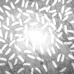
i

j

k

l

m

n

Figure 4:  The results of NPSA, PSA, EcoICA, DNJD, and SSF. The first and second column are the three source images and randomly-mixed images as the reference, respectively.

TABLE II:
Comparison of EcoICA, DNJD, SSF, PSA and NPSA for the ISI index of five different combinations. An average result of ten runs is computed.

Combination	EcoICA	DNJD	SSF	PSA	NPSA
1	0.0043	0.2375	0.1123	0.0061	$\bf 0.0031$
2	0.0309	0.3861	0.0656	0.0363	$\bf 0.0193$
3	$\bf 0.0122$	0.1353	0.0179	0.0186	0.0151
4	0.0309	0.1119	0.1238	0.0335	$\bf 0.0196$
5	0.0027	0.l923	0.0458	0.0035	0.0004

TABLE III:
Comparison of EcoICA, DNJD, SSF, PSA and NPSA for the TMSE index of five different combinations. An average result of ten runs is computed.

Combination	EcoICA	DNJD	SSF	PSA	NPSA
1	$2.6416\cdot 10^{-15}$	$2.5130\cdot 10^{-11}$	$2.6011\cdot 10^{-16}$	$6.7102\cdot 10^{-15}$	$\bf 2.4090\cdot 10^{-16}$
2	$6.2017\cdot 10^{-13}$	$3.0427\cdot 10^{-11}$	$\bf 1.5112\cdot 10^{-15}$	$1.0104\cdot 10^{-12}$	$1.5827\cdot 10^{-15}$
3	$2.3501\cdot 10^{-14}$	$3.4753\cdot 10^{-11}$	$1.1480\cdot 10^{-12}$	$3.4730\cdot 10^{-14}$	$\bf 1.9547\cdot 10^{-14}$
4	$6.2017\cdot 10^{-13}$	$6.3559\cdot 10^{-12}$	$1.5100\cdot 10^{-15}$	$1.0025\cdot 10^{-12}$	$\bf 1.4332\cdot 10^{-15}$
5	$2.4311\cdot 10^{-15}$	$1.2730\cdot 10^{-10}$	$6.2264\cdot 10^{-17}$	$8.6409\cdot 10^{-17}$	$\bf 6.1932\cdot 10^{-19}$

V-A2 Total mean square error ($\rm TMSE$)

TABLE IV:
Comparison of EcoICA, DNJD, SSF, PSA and NPSA for the correlation coefficient index of five different combinations. An average result of ten runs is computed.

Combination	EcoICA	DNJD	SSF	PSA	NPSA
1	0.9972	0.9230	0.9978	0.9969	0.9997
	0.9992	0.8596	0.9944	0.9992	0.9992
	1.0000	0.9637	0.9969	0.9998	1.0000
2	1.0000	0.9611	0.9963	0.9990	0.9985
	0.9553	0.8848	0.9872	0.9580	0.9988
	0.9988	0.9517	0.9989	0.9986	0.9989
3	0.9916	0.9451	0.9909	0.9902	0.9920
	1.0000	0.9760	0.9997	0.9999	1.0000
	0.9977	0.9252	0.9871	0.9972	0.9995
4	0.9988	0.9623	0.9972	0.9987	0.9989
	0.9553	0.8300	0.9632	0.9611	0.9989
	1.0000	0.9466	0.9935	0.9992	0.9983
5	1.0000	0.6621	0.9616	0.9998	1.0000
	1.0000	0.9906	0.9922	0.9998	1.0000
	0.9972	0.9156	0.9968	0.9966	0.9997

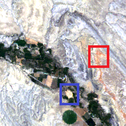
Figure 5:  True color image of the multispectral data.(R:band $3$, G:band $2$, B:band $1$).

To compute the error between the source image $\mathbf{I}$ and the separated image $\hat{\mathbf{I}}$, we use the mean square error (MSE) index. The images are first normalized into one length to eliminate the influence of the magnitude of the images, which can be implemented by $\mathbf{I}=\mathbf{I}/\|\mathbf{I}\|_{\mathrm{F}}$. Then, assume that the number of the pixels is $N$, the MSE index can be calculated by

$$\rm MSE=\frac{1}{N}\|\mathbf{I}-\hat{\mathbf{I}}\|_{F}^{2},$$ (48)

after computing the respective error of the three images, we then compute the total mean square error (TMSE)

$$\rm TMSE=\frac{1}{3}\sum_{\it{i}=1}^{3}\rm MSE_{\it{i}}^{2}.$$ (49)

Similar to the ISI index, the smaller the TMSE is, the better the algorithm performs. We take the average value of 10 runs as the result. The comparison between these methods is listed in Table III.

The NPSA algorithm has the smallest TMSE in combination 1, 2, 4 and 5, while SSF is slightly better than NPSA in combination 3.

V-A3 correlation coefficient

Both ISI and TMSE mainly focus on the overall performance. Here, we use the correlation coefficient to measure the similarity between $\mathbf{I}$ and $\hat{\mathbf{I}}$, in detail. The two images are first vectorized into the vector $\mathbf{i}$ and $\hat{\mathbf{i}}$ (Note that the normalization operation used in TMSE index have no impact on the final result since the correlation coefficient mainly measure the angle between the two vectors). Then the correlation coefficient can be calculated by

$$\rho=\frac{\mathbf{i}\cdot\hat{\mathbf{i}}}{\|\mathbf{i}\|\cdot\|\hat{\mathbf{i}}\|}.$$ (50)

The results of the five combinations are listed in Table IV. It can be found that the correlation coefficient of NPSA is higher than that of the others in most of the results and has a more stable performance meanwhile.

Eventually, combining the comparison results of several indices, we can conclude that the proposed algorithm obtains a more accurate and robust performance in terms of BIS application.

V-B Experiments On Multispectral Data

In this experiment, a $30$-m resolution Landsat-$5$ image embedded in the Environment for Visualizing Images (ENVI) software is selected to evaluate the performance of NPSA. Three algorithms, including the classical FastICA, PSA and EcoICA, are compared in the following experiments. The other two algorithms compared in the BIS experiments are not included since they have either an unstable performance or an unbearable computational complexity for real multi/hyperspectral data.

The dataset contains six bands in $30$-m resolution, with band numbers $1$-$5$ and $7$ (ranging from $0.482$ to $2.2$ um). Band $6$ is a thermal band ($10.40$-$12.50$ um) with a much lower spatial resolution ($120$ m). Thus, it is usually not included. A subscene with a $256\times 256$ pixel size is selected as the test data and the true color image is shown in Fig. 5. In this area, the main land cover types include vegetation, water, bareland, etc.

In our experiment, we set the number of independent components to $p=6$, i.e., we select the full-band image to conduct the test. Eventually, we can obtain $6$ principal skewness components of the image and the results are shown in Fig. 6. IC$1$-$3$ are almost the same, which correspond to three main land cover types: vegetation, bareland and water, respectively. By inspection, the result of NPSA in Fig. 6. w (IC$2$) and Fig. 6. x (IC$6$) is also superior to that of the other algorithms.

It is worth taking IC$2$ and IC$6$ as an example to compare the differences of these algorithms once again. IC$2$ mainly corresponds to the cultivated farmland (e.g., framed in the blue rectangular), while IC$6$ corresponds to the uncultivated bareland (e.g., framed in the red rectangular). Their spectral curves are shown in Fig. 7. Because of the orthogonal constraint in PSA, EcoICA and FastICA, for the objects with similar spectra, there is often only one of them being highlighted. When the farmland is extracted as the independent component in IC$2$, the uncultivated bareland will be suppressed in the later component, as shown in Fig. 6. f, Fig. 6. l and Fig. 6. r. While in NPSA, because the restriction of orthogonal constraint is relaxed, the object that is spectrally similar to the previous components can still be likely to be detected. As shown in Fig. 6. x, the uncultivated bareland can still be efficiently extracted in NPSA.

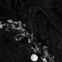
a IC1 of FastICA

b IC2 of FastICA

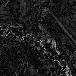
c IC3 of FastICA

d IC4 of FastICA

e IC5 of FastICA

f IC6 of FastICA

g IC1 of EcoICA

h IC2 of EcoICA

i IC3 of EcoICA

j IC4 of EcoICA

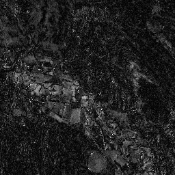
k IC5 of EcoICA

l IC6 of EcoICA

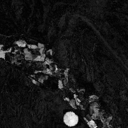
m IC1 of PSA

n IC2 of PSA

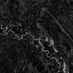
o IC3 of PSA

p IC4 of PSA

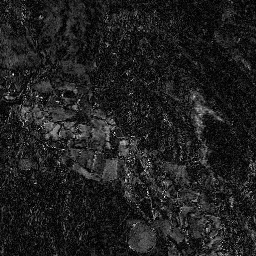
q IC5 of PSA

r IC6 of PSA

s IC1 of NPSA

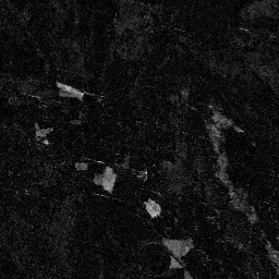
t IC2 of NPSA

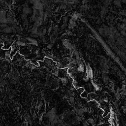
u IC3 of NPSA

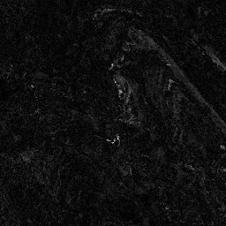
v IC4 of NPSA

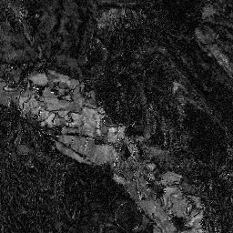
w IC5 of NPSA

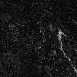
x IC6 of NPSA

Figure 6:  The results of FastICA, EcoICA, PSA and NPSA for the multispectral image.

To further demonstrate the advantage of NPSA, we conduct a quantitative comparison by calculating the skewness value of each independent component, and the results are plotted in Fig. 8. As can be seen, the skewness value of NPSA in each independent component is equal to or larger than that of the others, which implies that NPSA can obtain the more reasonable maxima in each unit and has a better overall performance.

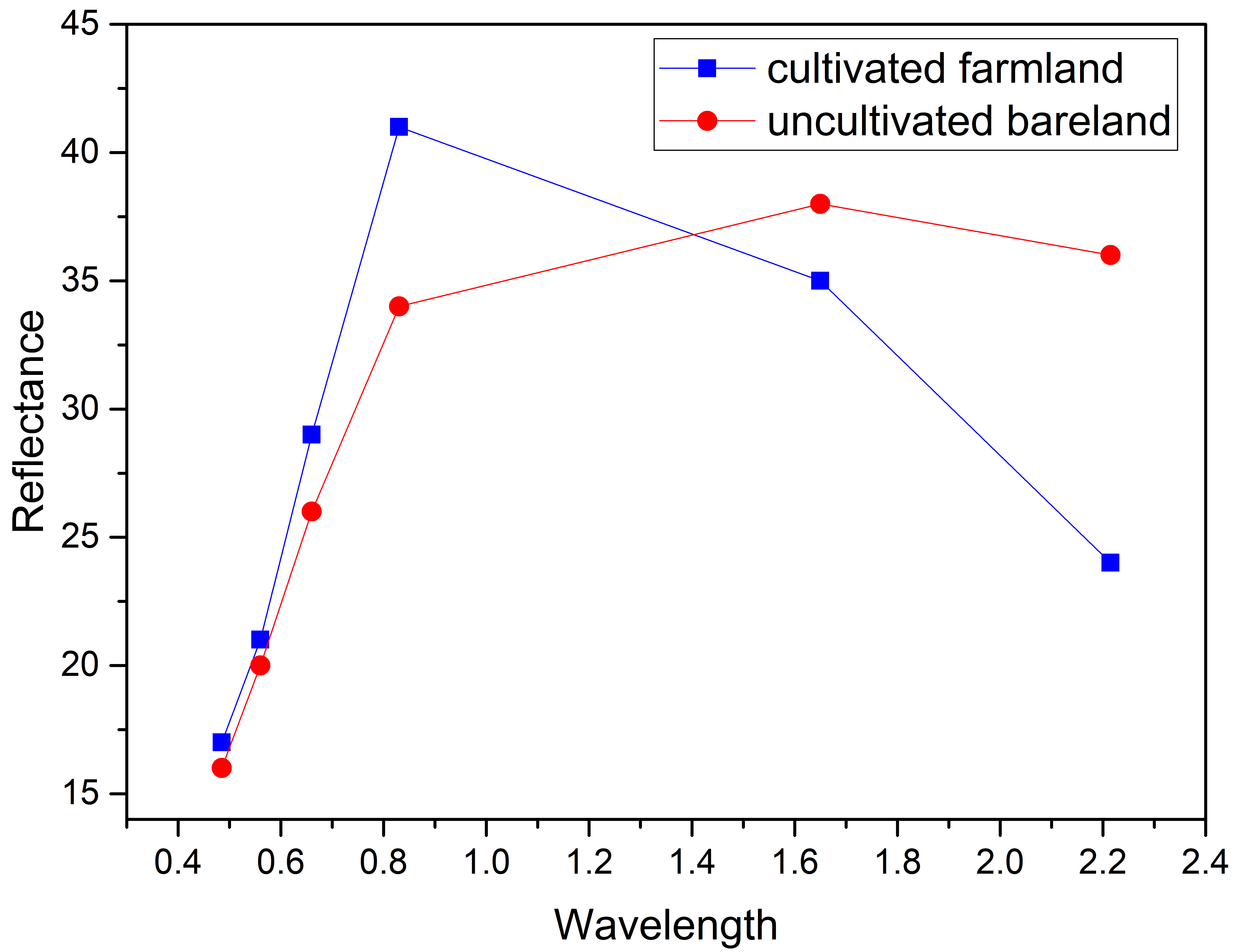
Figure 7:  The spectral comparison for the framland and the uncultivated bareland.

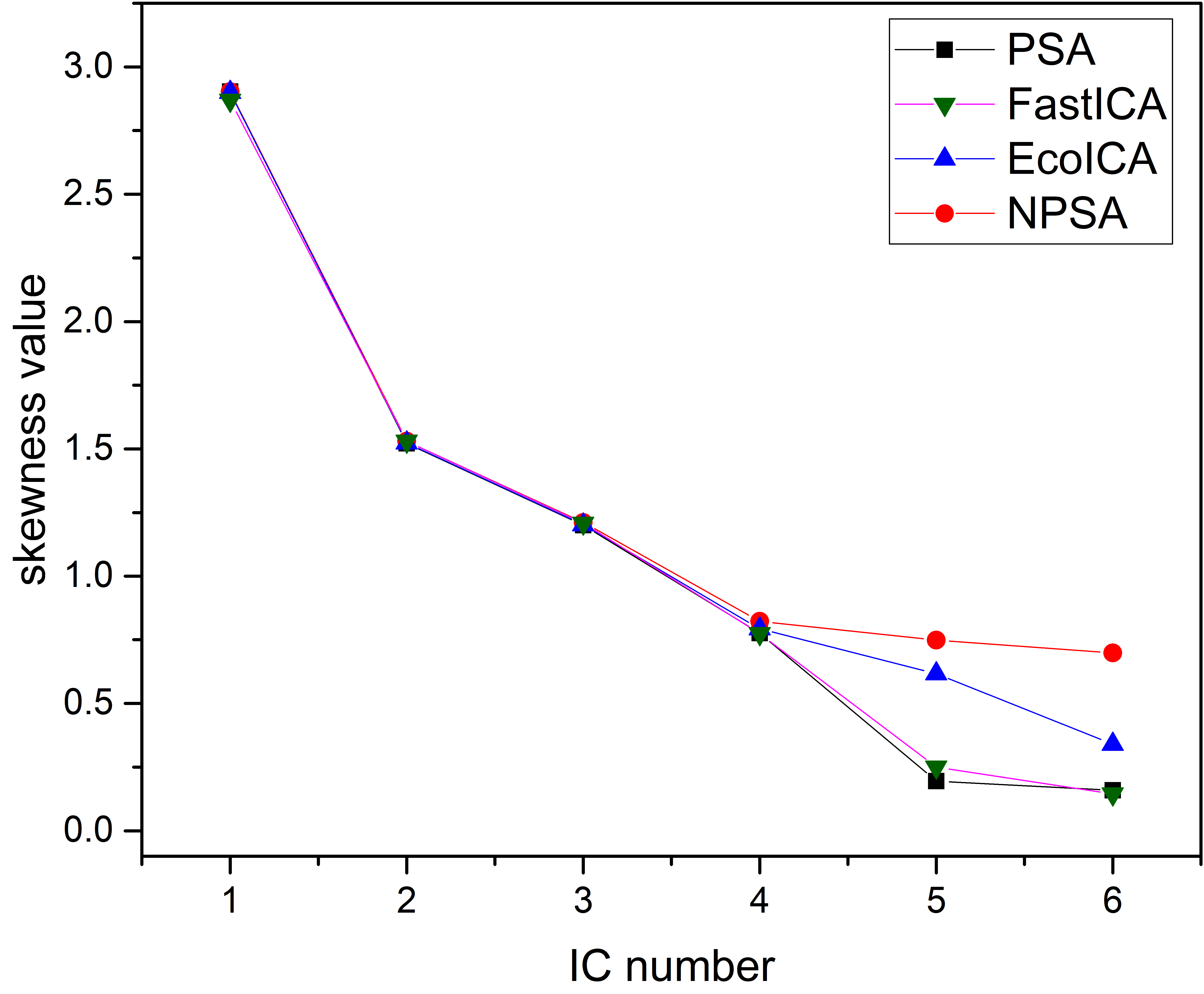
Figure 8:  Skewness comparison of FastICA, EcoICA, PSA and NPSA for the multispectral image.

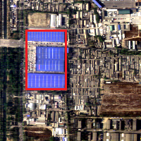
Figure 9:  True color image of the hyperspectral data. (R:$620$nm, G:$559$nm, B:$473$nm) .

a IC1 of FastICA
($\rm skew=4.7826$)

b IC2 of FastICA
($\rm skew=4.2132$)

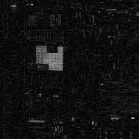
c IC3 of FastICA
($\rm skew=1.7656$)

d IC1 of EcoICA
($\rm skew=4.8943$)

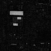
e IC2 of EcoICA
($\rm skew=4.1186$)

f IC3 of EcoICA
($\rm skew=2.8699$)

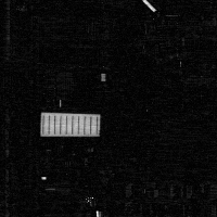
g IC1 of PSA
($\rm skew=4.7648$)

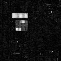
h IC2 of PSA
($\rm skew=4.2108$)

i IC3 of PSA
($\rm skew=2.1952$)

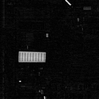
j IC1 of NPSA
($\rm skew=4.9410$)

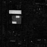
k IC2 of NPSA
($\rm skew=4.3176$)

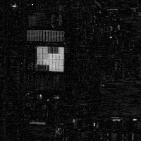
l IC3 of NPSA
($\rm skew=2.9675$)

Figure 10:  Some results of FastICA, EcoICA, PSA and NPSA for the hyperspectral image. The corresponding skewness value of each IC is also attached.

V-C Experiments On Hyperspectral Data

Here, the hyperspectral image data we used to test the method is from the Operational Modular Imaging Spectrometer-II, which were acquired by the Aerial Photogrammetry and Remote Sensing Bureau in Beijing, China, in $2000$. It includes $64$ bands from visible to thermal infrared with about $3$-m spatial resolution and $10$-nm spectral resolution and has $200\times 200$ pixels in each band. Since the signal-to-noise ratio is low in bands $55$-$60$, we select the remaining $58$ bands as our test data. The true color image is shown in Fig. 9. The red rectangular framed in Fig. 9 is an area of blue-painted roof. After a field investigation, it was found that the roof was made from three different materials although there is no obvious difference in the visible band.

We display the results of feature extraction in Fig. 10 and plot the curves of skewness in Fig. 11. All algorithms can automatically extract the three different materials as the independent components. The skewness comparison both attached in Fig. 10 for the three ICs and in Fig. 11 for all the ICs can also demonstrate that NPSA outperforms the other three algorithms. It can be observed that in Fig. 11, the skewness of IC$2$ and IC$6$ extracted by EcoICA is slightly larger than that of NPSA. However, we can still conclude that NPSA has the better overall performance.

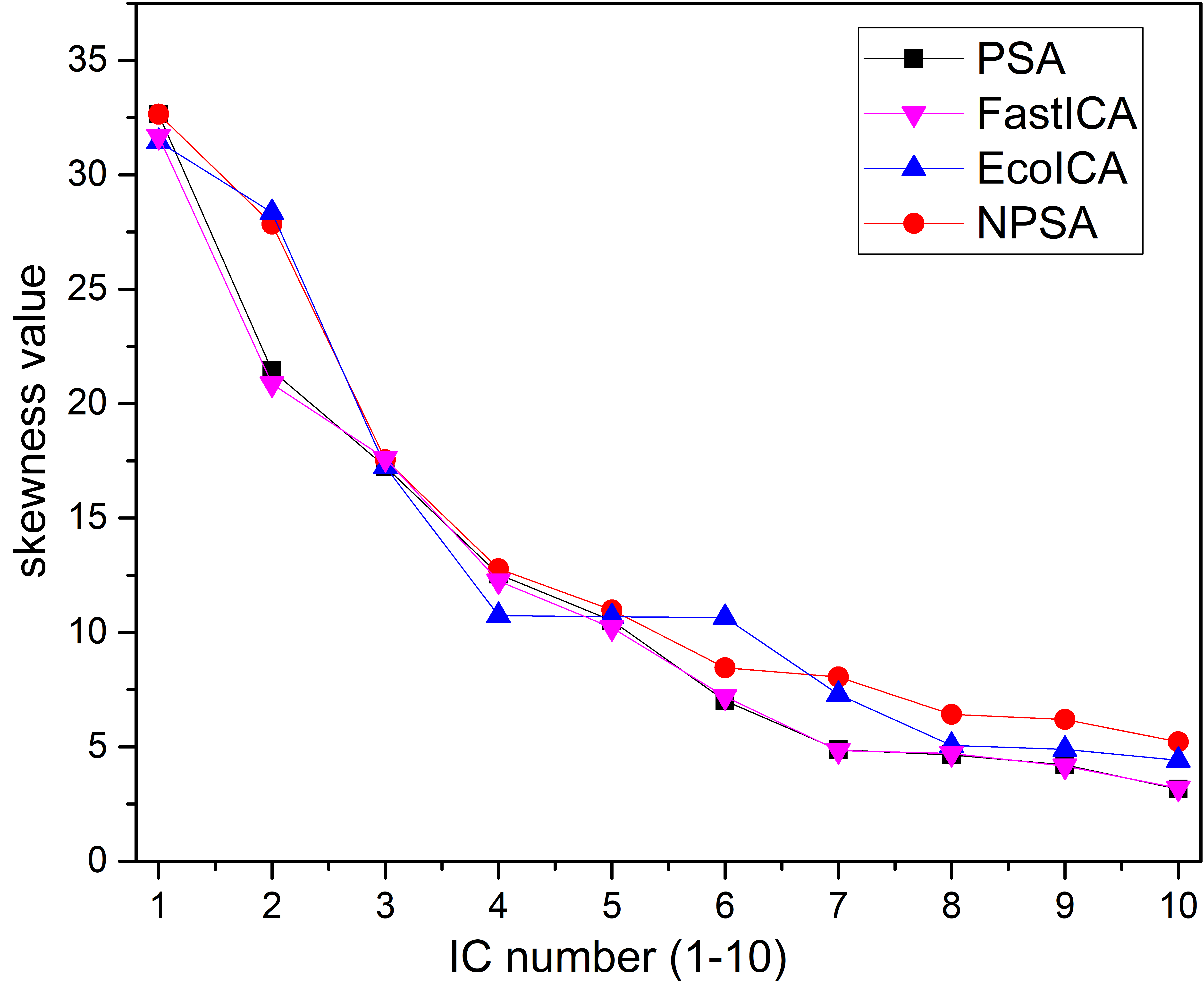
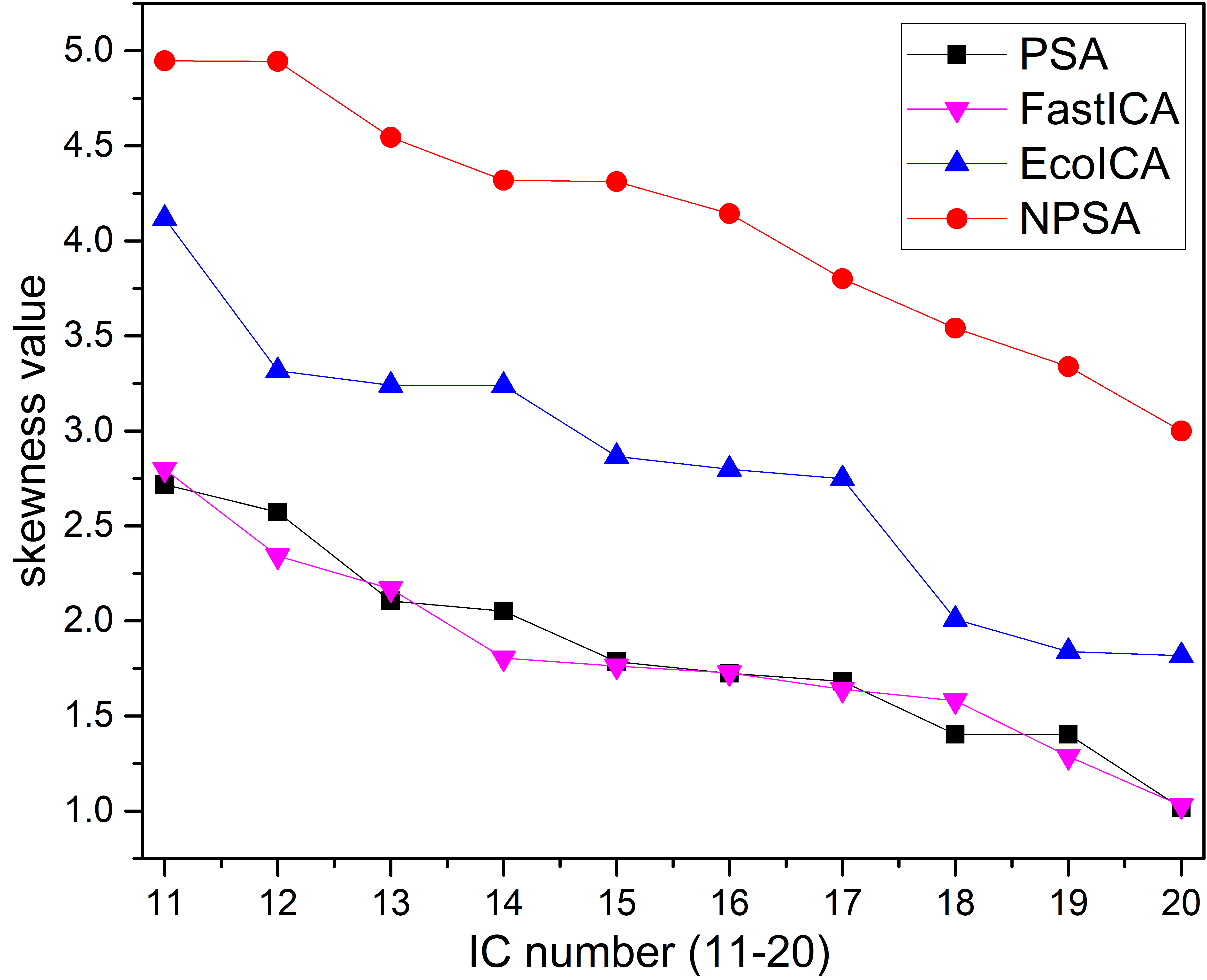
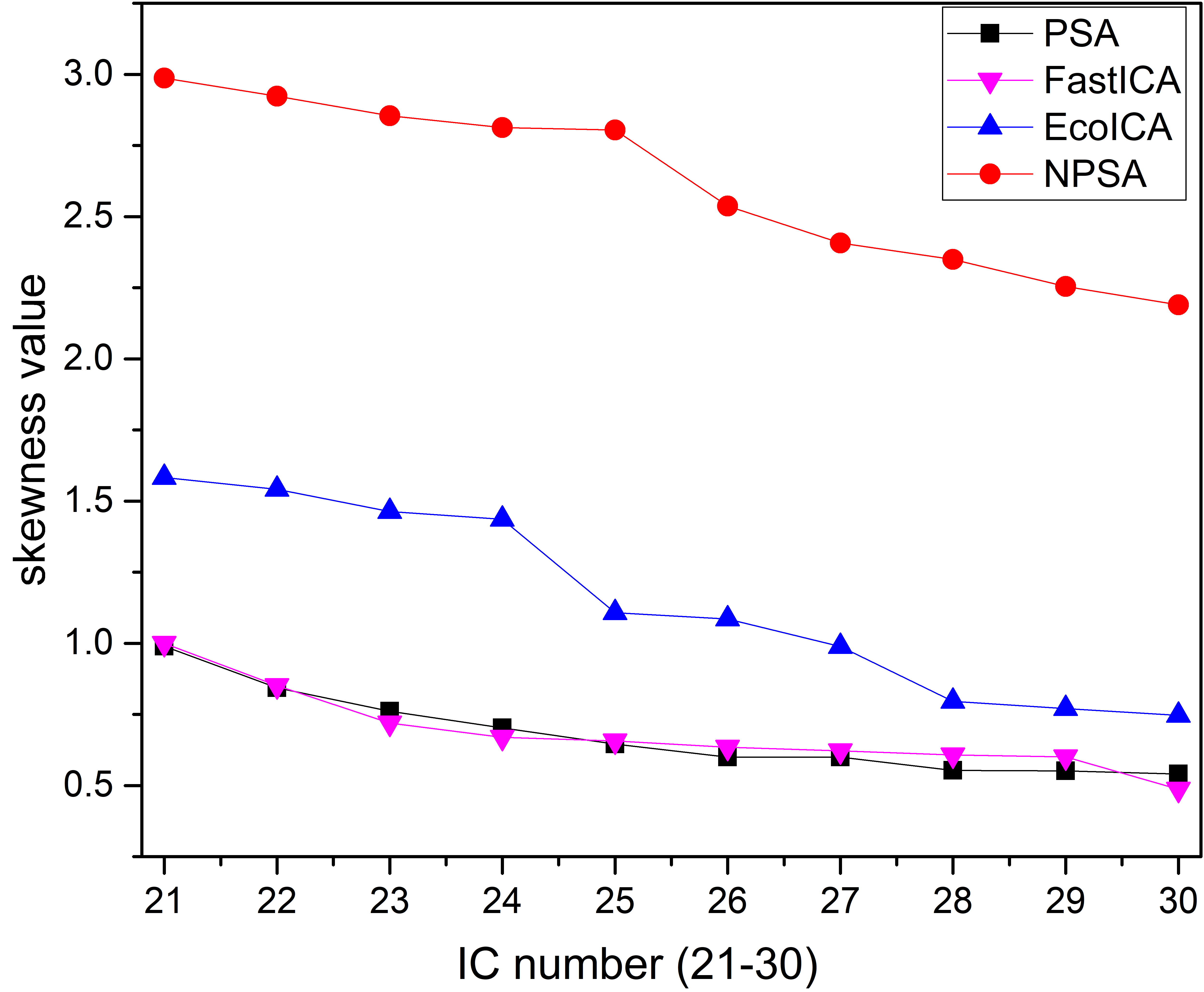
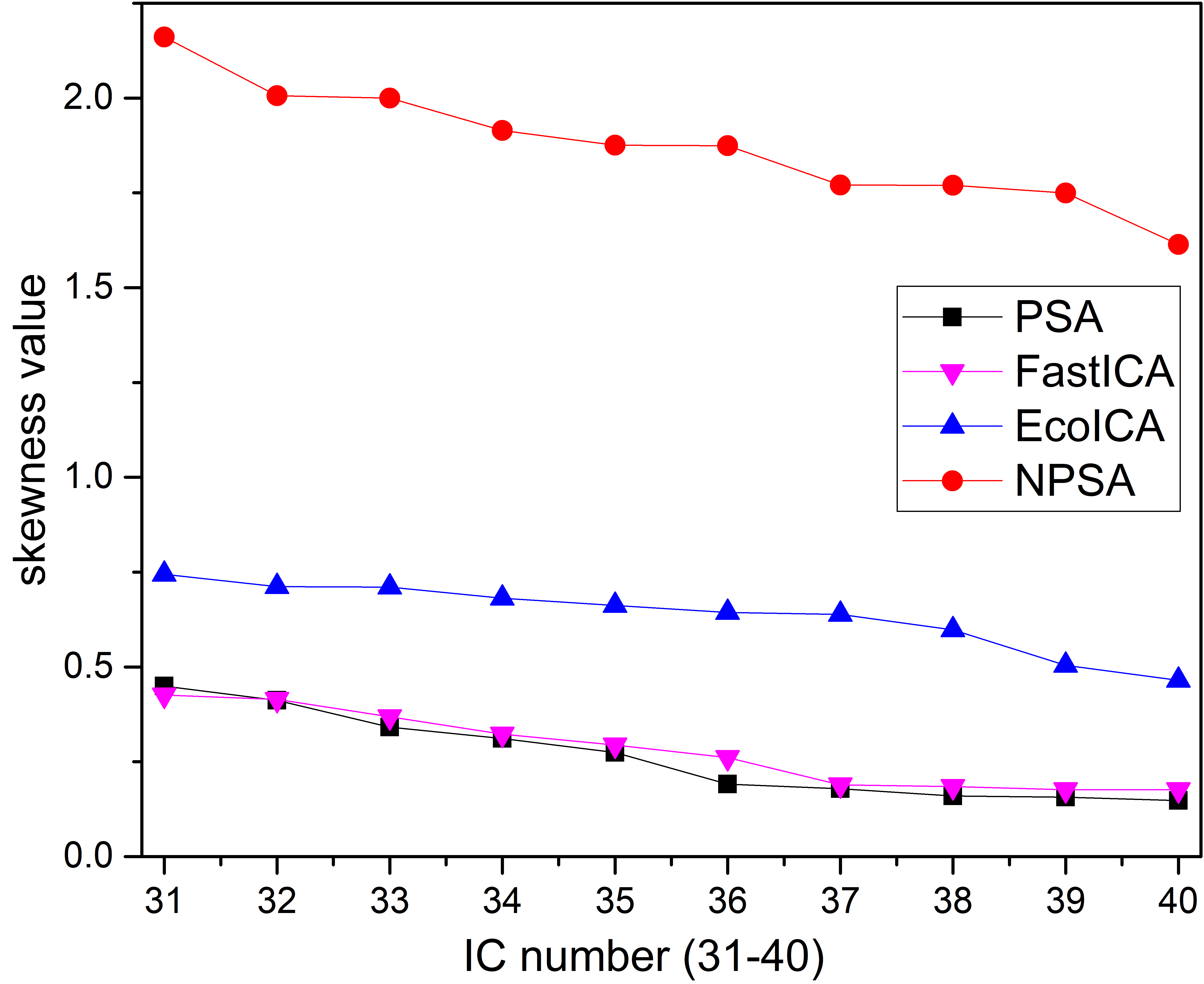
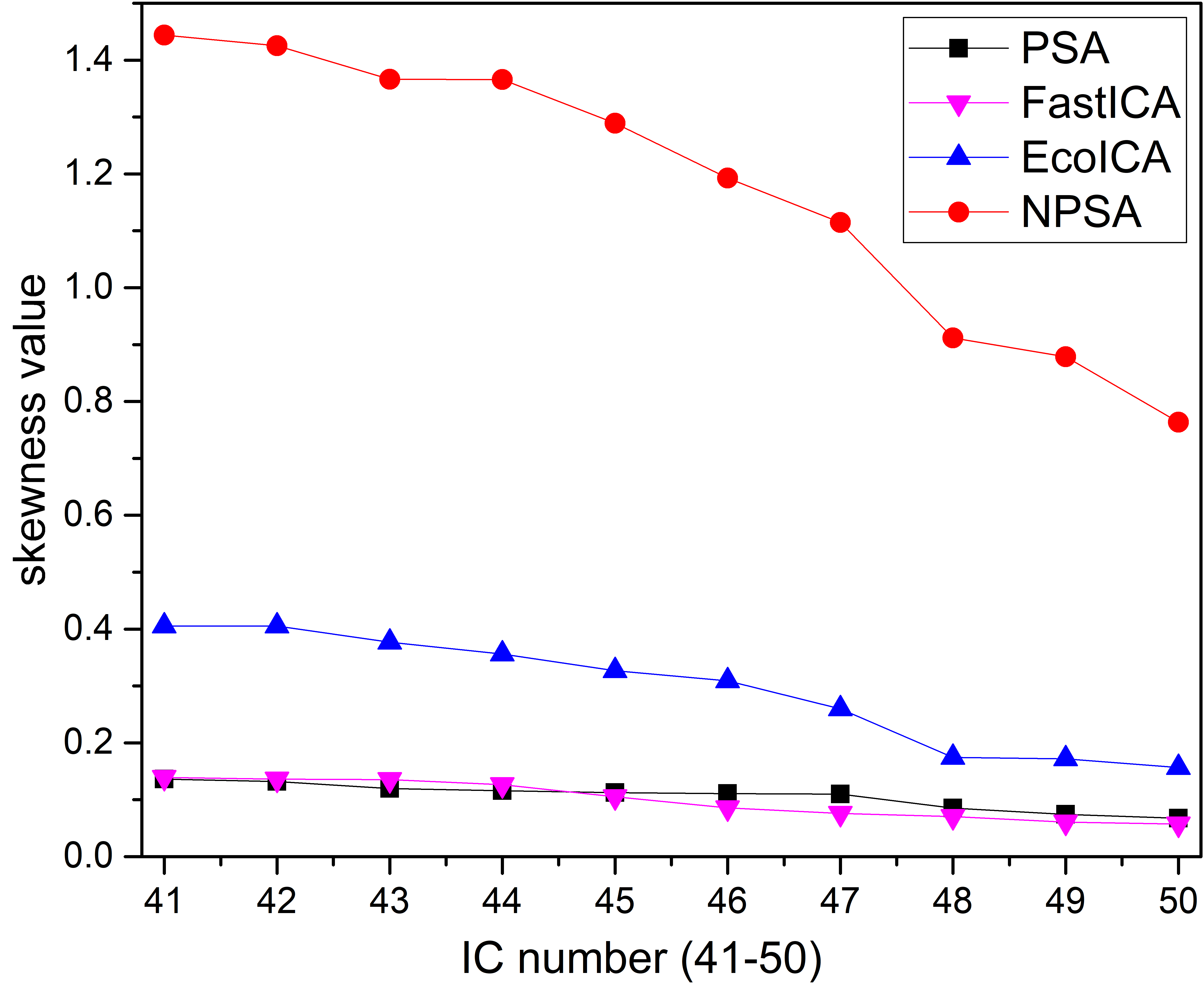
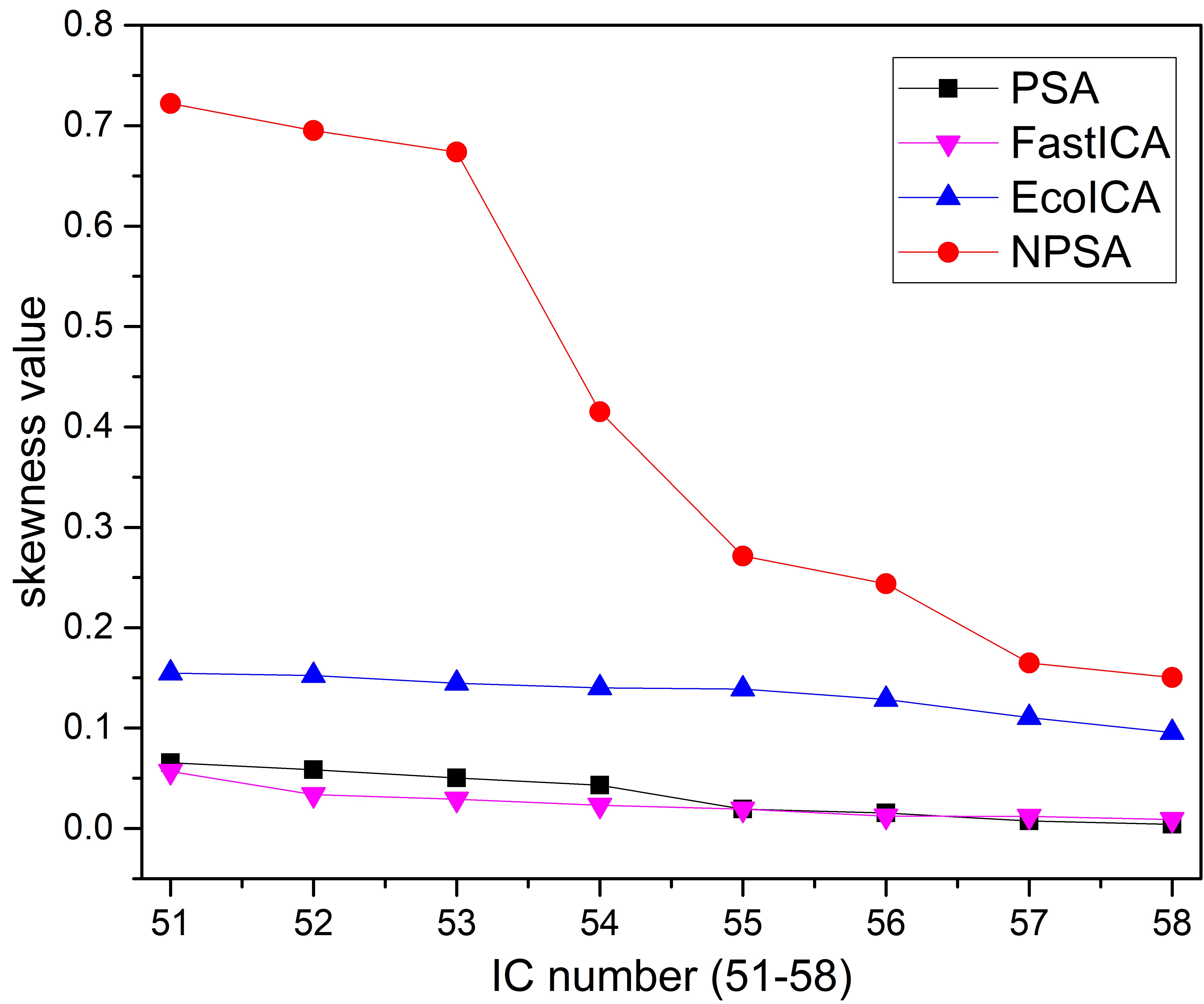
Figure 11:  Skewness comparison of FastICA, EcoICA, PSA and NPSA for the hyperspectral image.

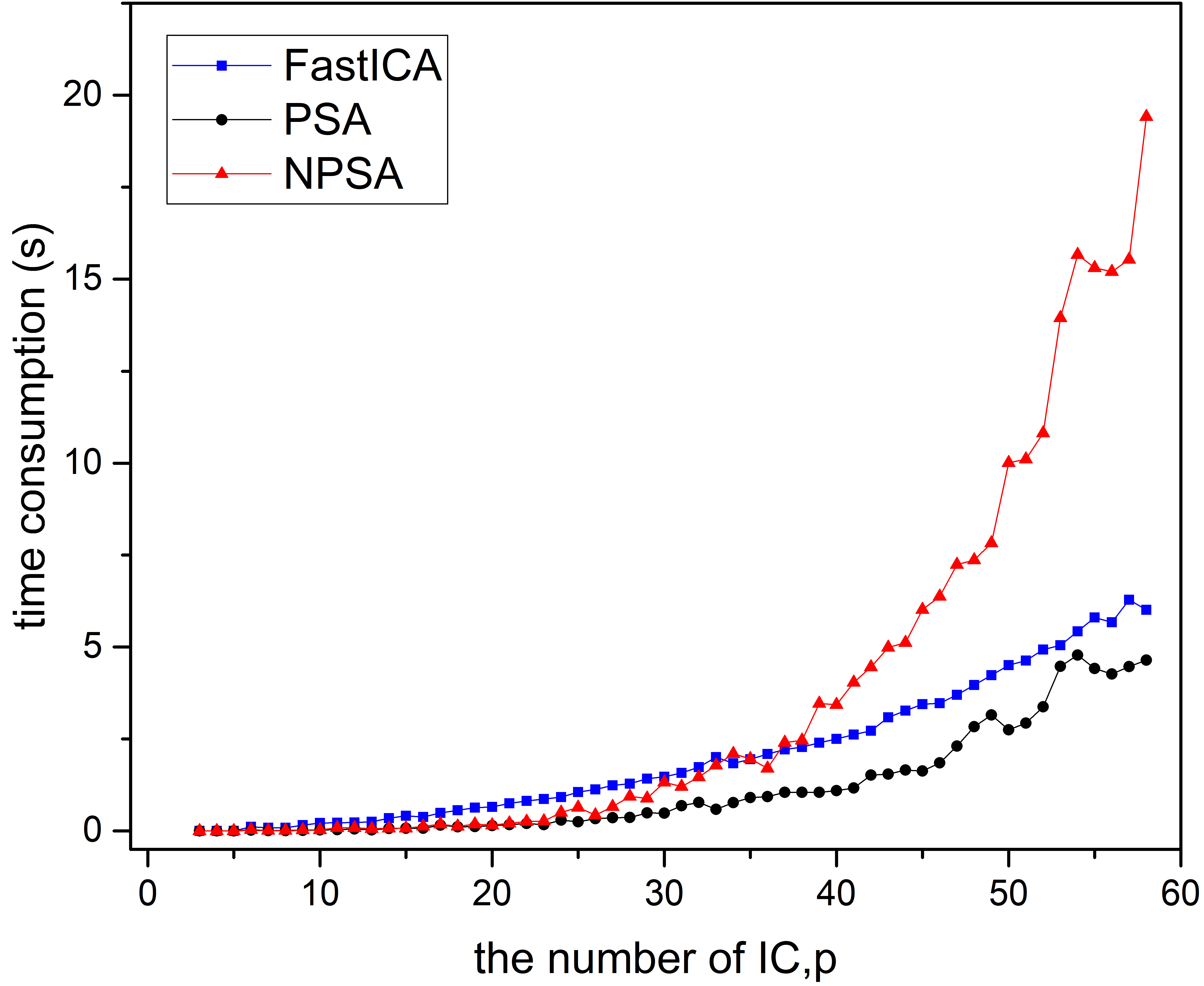
Figure 12:  Time consumption comparison of FastICA, PSA and NPSA as a function of the number of ICs.

Besides, a time efficiency comparison is also conducted in this experiment. The number of ICs, i.e, $p$, ranges from $6$ to $58$ and the time curve as a function of $p$ is plotted in Fig. 12. As $p$ increases, the time consumption of NPSA is greater than that of PSA. This is because we need to update the tensor in each unit of NPSA while this repeated computation in PSA can be simplified [24]. However, the time of NPSA for a full-band data set, i.e., $p=58$, is about $19$ seconds, which is still efficient and acceptable for the real hyperspectral image. Note that since the time of EcoICA for a full-band data set is about $60$ seconds, which is much larger than that of the other three algorithms, so we do not take it into our comparison in this experiment. To sum up, our algorithm can obtain a higher accuracy in the sacrifice of some time efficiency at an acceptable level.

VI Conclusion

Orthogonal complement constraint is a widely used strategy to prevent the solution to be determined from converging to the previous ones[24, 25, 18]. However, such a constraint can be irreconcilably contradicted with the inherent nonorthogonality of supersymmetric tensor. In this paper, originated from PSA, we have proposed a new algorithm, which is named nonorthogonal principal skewness analysis (NPSA). In NPSA, a more relaxed constraint than the orthogonal constraint is proposed to search for the locally maximum skewness direction in a larger space, and thus we can obtain the more accurate results. A detailed theoretical analysis is also presented to justify its validity. Furthermore, it is interesting to find that the differences of PSA and NPSA lie in the order in which they perform the orthogonal complement projection and the $n$-mode operation. We first apply the algorithm into the BIS probelm and several accuracy metrics evaluated in our experiments show that NPSA can obtain a more accurate and robust result. Experiments for real multi/hyperspectral data also demonstrate that NPSA outperforms the other algorithms in extracting the ICs of the image.

On the one hand, our method can be extended to fourth-or-higher-order case naturally. Both PSA and NPSA focus on the skewness index, which may not be always the best choice to describe the statistical structure of the data. Kurtosis and other indices can be considered as the alternative. On the other hand, NPSA needs to update the coskewness tensor in each unit, which makes it slightly more time-consuming than PSA. So in the future, more efficient optimization methods will be worth studying.

References

- [1] X. Geng, K. Sun, L. Ji, Y. Zhao, and H. Tang. Optimizing the endmembers using volume invariant constrained model. IEEE Transactions on Image Processing, 24(11):3441–3449, 2015.
- [2] Yuntao Qian, Fengchao Xiong, Shan Zeng, Jun Zhou, and Yuan Yan Tang. Matrix-vector nonnegative tensor factorization for blind unmixing of hyperspectral imagery. IEEE Transactions on Geoscience and Remote Sensing, 55(3):1776–1792, 2017.
- [3] Chein I Chang, Xiao Li Zhao, M. L. G Althouse, and Jeng Jong Pan. Least squares subspace projection approach to mixed pixel classification for hyperspectral images. IEEE Transactions on Geoscience and Remote Sensing, 36(3):898–912, 1998.
- [4] Baofeng Guo, S. R. Gunn, R. I. Damper, and J. D. B. Nelson. Customizing kernel functions for svm-based hyperspectral image classification. IEEE Transactions on Image Processing A Publication of the IEEE Signal Processing Society, 17(4):622–629, 2008.
- [5] Z. Zou and Z. Shi. Random access memories: A new paradigm for target detection in high resolution aerial remote sensing images. IEEE Transactions on Image Processing A Publication of the IEEE Signal Processing Society, PP(99):1–1, 2018.
- [6] Ting Wang, Bo Du, and Liangpei Zhang. A kernel-based target-constrained interference-minimized filter for hyperspectral sub-pixel target detection. IEEE Journal of Selected Topics in Applied Earth Observations and Remote Sensing, 6(2):626–637, 2013.
- [7] Weiwei Sun and Qian Du. Graph-regularized fast and robust principal component analysis for hyperspectral band selection. IEEE Transactions on Geoscience and Remote Sensing, PP(99):1–11, 2018.
- [8] H Hotelling. Analysis of a complex of statistical variables into principal components. Journal of Educational Psychology, 24(6):417–520, 1933.
- [9] Bernhard Schölkopf, Alexander Smola, and Klaus-Robert Müller. Kernel principal component analysis. In International Conference on Artificial Neural Networks, pages 583–588. Springer, 1997.
- [10] Andrew A Green, Mark Berman, Paul Switzer, and Maurice D Craig. A transformation for ordering multispectral data in terms of image quality with implications for noise removal. IEEE Transactions on geoscience and remote sensing, 26(1):65–74, 1988.
- [11] Xiurui Geng, Kang Sun, Luyan Ji, and Yongchao Zhao. A high-order statistical tensor based algorithm for anomaly detection in hyperspectral imagery. Scientific reports, 4:6869, 2014.
- [12] Yanfeng Gu, Ying Liu, and Ye Zhang. A selective kpca algorithm based on high-order statistics for anomaly detection in hyperspectral imagery. IEEE Geoscience and Remote Sensing Letters, 5(1):43–47, 2008.
- [13] Shih Yu Chu, Hsuan Ren, and Cheini Chang. High-order statistics-based approaches to endmember extraction for hyperspectral imagery. Proceedings of SPIE - The International Society for Optical Engineering, 6966, 2008.
- [14] Hsuan Ren, Qian Du, Jing Wang, and Chein-I Chang. Automatic target recognition for hyperspectral imagery using high-order statistics. Aerospace and Electronic Systems IEEE Transactions on, 42(4):1372–1385, 2006.
- [15] Xiurui Geng, Luyan Ji, Yongchao Zhao, and Fuxiang Wang. A small target detection method for the hyperspectral image based on higher order singular value decomposition (hosvd). IEEE Geoscience and Remote Sensing Letters, 10(6):1305–1308, 2013.
- [16] A. Hyvarinen and E. Oja. Independent component analysis: algorithms and applications. Neural Networks, 13(4):411–430, 2000.
- [17] J. F Cardoso and A Souloumiac. Blind beamforming for non gaussian signals. IEE Proc.-F, 140(6):362–370, 1993.
- [18] Aapo Hyvarinen. Fast and robust fixed-point algorithms for independent component analysis. IEEE transactions on Neural Networks, 10(3):626–634, 1999.
- [19] Liyan Song and Haiping Lu. Ecoica: Skewness-based ica via eigenvectors of cumulant operator. In Asian Conference on Machine Learning, pages 445–460, 2016.
- [20] A-J Van Der Veen. Joint diagonalization via subspace fitting techniques. In Acoustics, Speech, and Signal Processing, 2001. Proceedings.(ICASSP’01). 2001 IEEE International Conference on, volume 5, pages 2773–2776. IEEE, 2001.
- [21] Fuxiang Wang, Zhongkan Liu, and Jun Zhang. Nonorthogonal joint diagonalization algorithm based on trigonometric parameterization. IEEE Transactions on Signal Processing, 55(11):5299–5308, Nov 2007.
- [22] A. Yeredor. Non-orthogonal joint diagonalization in the least-squares sense with application in blind source separation. IEEE Transactions on Signal Processing, 50(7):1545–1553, Jul 2002.
- [23] E Oja and Zhijian Yuan. The fastica algorithm revisited: Convergence analysis. IEEE Transactions on Neural Networks, 17(6):1370–1381, 2006.
- [24] Xiurui Geng, Luyan Ji, and Kang Sun. Principal skewness analysis: algorithm and its application for multispectral/hyperspectral images indexing. IEEE Geoscience and Remote Sensing Letters, 11(10):1821–1825, 2014.
- [25] Xiurui Geng, Lingbo Meng, Lin Li, Luyan Ji, and Kang Sun. Momentum principal skewness analysis. IEEE Geoscience and Remote Sensing Letters, 12(11):2262–2266, 2015.
- [26] Lingbo Meng, Xiurui Geng, and Luyan Ji. Principal kurtosis analysis and its application for remote-sensing imagery. International Journal of Remote Sensing, 37(10):2280–2293, 2016.
- [27] Ariel Jaffe, Roi Weiss, and Boaz Nadler. Newton correction methods for computing real eigenpairs of symmetric tensors. 2017.
- [28] Animashree Anandkumar, Rong Ge, Daniel Hsu, Sham M Kakade, and Matus Telgarsky. Tensor decompositions for learning latent variable models. The Journal of Machine Learning Research, 15(1):2773–2832, 2014.
- [29] Tamara G Kolda and Brett W Bader. Tensor decompositions and applications. SIAM review, 51(3):455–500, 2009.
- [30] Charles F. Van Loan. The ubiquitous kronecker product. Journal of Computational and Applied Mathematics, 123(1):85–100, 2000.
- [31] Xian-Da Zhang. Matrix analysis and applications. Cambridge University Press, 2017.
- [32] Lek-Heng Lim. Singular values and eigenvalues of tensors: a variational approach. In Computational Advances in Multi-Sensor Adaptive Processing, 2005 1st IEEE International Workshop on, pages 129–132. IEEE, 2005.
- [33] Liqun Qi. Eigenvalues of a real supersymmetric tensor. Journal of Symbolic Computation, 40(6):1302–1324, 2005.
- [34] Eric Moreau and Odile Macchi. A one stage self-adaptive algorithm for source separation. In Acoustics, Speech, and Signal Processing, 1994. ICASSP-94., 1994 IEEE International Conference on, volume 3, pages III–49. IEEE, 1994.