Solving quadratic matrix equations arising in random walks in the quarter planethanks: Research partially supported by INdAM-GNCS

Dario A. Bini Dipartimento di Matematica, Università di Pisa, Italy, () dario.bini@unipi.it    Beatrice Meini Dipartimento di Matematica, Università di Pisa, Italy, () beatrice.meini@unipi.it    Jie Meng Department of Mathematics, Pusan National University, Busan, South Korea () mengjie@pusan.ac.kr
Abstract

Quadratic matrix equations of the kind A1X2+A0X+A1=Xsubscript𝐴1superscript𝑋2subscript𝐴0𝑋subscript𝐴1𝑋A_{1}X^{2}+A_{0}X+A_{-1}=X are encountered in the analysis of Quasi–Birth-Death stochastic processes where the solution of interest is the minimal nonnegative solution G𝐺G. In many queueing models, described by random walks in the quarter plane, the coefficients A1,A0,A1subscript𝐴1subscript𝐴0subscript𝐴1A_{1},A_{0},A_{-1} are infinite tridiagonal matrices with an almost Toeplitz structure. Here, we analyze some fixed point iterations, including Newton’s iteration, for the computation of G𝐺G and introduce effective algorithms and acceleration strategies which fully exploit the Toeplitz structure of the matrix coefficients and of the current approximation. Moreover, we provide a structured perturbation analysis for the solution G𝐺G. The results of some numerical experiments which demonstrate the effectiveness of our approach are reported.

Keywords: Matrix equations, random walks, Markov chains, Toeplitz matrices, infinite matrices, fixed point iteration, Newton iteration.

MSC: 65F30, 15A24, 60J22, 15B05

1 Introduction

Random walks in the quarter plane describe a wide variety of two-queue models with various service policies such as nonpreemptive priority, K𝐾K-limited service, server vacation and server setup [26]. Models of this kind concern, for instance, bi-lingual call centers [30], generalized two-node Jackson networks [27], two-demand models [10], two-stage inventory queues [11], and more.

A theoretical analysis of stability, of tail decay rates and of other asymptotic properties has been carried out by several authors, in particular in [14], [22], [23], [26], and in the book [9], in which the invariant measure and the transient behavior are investigated by means of analytic and functional tools.

A different approach is based on representing a random walk in the quarter plane as a 2-dimensional Quasi–Birth-Death (QBD) stochastic process. This latter framework, based on the matrix analytic approach of [25], allows to express the invariant probability measure, and other quantities of interest for the stochastic model, in terms of a solution of suitable quadratic matrix equations. This provides a further tool for the theoretical analysis [17], [19] and paves the way for the design of effective algorithms based on the numerical solution of quadratic matrix equations.

In fact, relying on the matrix analytic theory of [25], the problem of computing the invariant probability measure of a QBD process is reduced to computing the minimal nonnegative solution G𝐺G and R𝑅R of the two matrix equations

(1) A1X2+A0X+A1=X,subscript𝐴1superscript𝑋2subscript𝐴0𝑋subscript𝐴1𝑋\displaystyle A_{1}X^{2}+A_{0}X+A_{-1}=X,
(2) A1+XA0+X2A1=X,subscript𝐴1𝑋subscript𝐴0superscript𝑋2subscript𝐴1𝑋\displaystyle A_{1}+XA_{0}+X^{2}A_{-1}=X,

respectively, where the coefficients A1,A0,A1subscript𝐴1subscript𝐴0subscript𝐴1A_{-1},A_{0},A_{1} are nonnegative matrices such that A1+A0+A1subscript𝐴1subscript𝐴0subscript𝐴1A_{-1}+A_{0}+A_{1} is row-stochastic and X𝑋X is the unknown. We say that a matrix X𝑋X is nonnegative, and we write X0𝑋0X\geq 0, if its entries are nonnegative. Moreover we say that a solution X𝑋X of a matrix equation is minimal nonnegative if X0𝑋0X\geq 0 and for any other nonnegative solution Y𝑌Y it holds YX0𝑌𝑋0Y-X\geq 0. For more details in this regard, we refer the reader to the books [2], [19], and [25].

In the case where the coefficients are finite dimensional, several algorithms have been introduced to compute G𝐺G and R𝑅R. They include fixed point iterations and doubling algorithms like Logarithmic Reduction and Cyclic Reduction (CR) [7], [2], [19].

In the case of 2-dimensional QBDs the coefficients A1,A0subscript𝐴1subscript𝐴0A_{-1},A_{0}, A1subscript𝐴1A_{1} are semi-infinite and have a special structure, more precisely,

(3) Ai=[bi,0bi,1ai,1ai,0ai,1ai,1ai,0ai,1],i=1,0,1,formulae-sequencesubscript𝐴𝑖matrixsubscript𝑏𝑖0subscript𝑏𝑖1subscript𝑎𝑖1subscript𝑎𝑖0subscript𝑎𝑖1missing-subexpressionsubscript𝑎𝑖1subscript𝑎𝑖0subscript𝑎𝑖1missing-subexpressionmissing-subexpression𝑖101A_{i}=\begin{bmatrix}b_{i,0}&b_{i,1}\\ a_{i,-1}&a_{i,0}&a_{i,1}\\ &a_{i,-1}&a_{i,0}&a_{i,1}\\ &&\ddots&\ddots&\ddots\\ \end{bmatrix},\quad i=-1,0,1,

where ai,j0subscript𝑎𝑖𝑗0a_{i,j}\geq 0, bi,j0subscript𝑏𝑖𝑗0b_{i,j}\geq 0 and i,j=11ai,j=1superscriptsubscript𝑖𝑗11subscript𝑎𝑖𝑗1\sum_{i,j=-1}^{1}a_{i,j}=1, i=11j=01bi,j=1superscriptsubscript𝑖11superscriptsubscript𝑗01subscript𝑏𝑖𝑗1\sum_{i=-1}^{1}\sum_{j=0}^{1}b_{i,j}=1. These blocks belong to the class of matrices representable in the form A=T(s)+E𝐴𝑇𝑠𝐸A=T(s)+E where T(s)𝑇𝑠T(s) is the Toeplitz matrix associated with the symbol s(z)=isizi𝑠𝑧subscript𝑖subscript𝑠𝑖superscript𝑧𝑖s(z)=\sum_{i\in\mathbb{Z}}s_{i}z^{i}, that is, (T(s))i,j=sjisubscript𝑇𝑠𝑖𝑗subscript𝑠𝑗𝑖(T(s))_{i,j}=s_{j-i}, and E=(ei,j)𝐸subscript𝑒𝑖𝑗E=(e_{i,j}) is such that vi=j|ei,j|subscript𝑣𝑖subscript𝑗subscript𝑒𝑖𝑗v_{i}=\sum_{j}|e_{i,j}| is finite and limivi=0subscript𝑖subscript𝑣𝑖0\lim_{i}v_{i}=0. The matrix T(s)𝑇𝑠T(s) is called Toeplitz part while E𝐸E is called correction. Here s(z)𝑠𝑧s(z) is a function belonging to the Wiener class 𝒲={f(z)=ifizi,fw:=i|fi|<}𝒲formulae-sequence𝑓𝑧subscript𝑖subscript𝑓𝑖superscript𝑧𝑖assignsubscriptnorm𝑓𝑤subscript𝑖subscript𝑓𝑖\mathcal{W}=\{f(z)=\sum_{i\in\mathbb{Z}}f_{i}z^{i},~{}\|f\|_{w}:=\sum_{i\in\mathbb{Z}}|f_{i}|<\infty\}. In particular, for the matrix in (3) it is easy to check that Ai=T(ai)+Eisubscript𝐴𝑖𝑇subscript𝑎𝑖subscript𝐸𝑖A_{i}=T(a_{i})+E_{i} where ai(z)=j=11ai,jzjsubscript𝑎𝑖𝑧superscriptsubscript𝑗11subscript𝑎𝑖𝑗superscript𝑧𝑗a_{i}(z)=\sum_{j=-1}^{1}a_{i,j}z^{j} and Eisubscript𝐸𝑖E_{i} has zero entries except for the first row which is equal to [bi,0ai,0,bi,1ai,1,0,]subscript𝑏𝑖0subscript𝑎𝑖0subscript𝑏𝑖1subscript𝑎𝑖10[b_{i,0}-a_{i,0},b_{i,1}-a_{i,1},0,\ldots]. Matrices of this kind are called Quasi-Toeplitz (QT) in [3].

The case of QBD with infinite blocks has been initially investigated in [17], [18], and [20], by reducing the problem to finite size relying on truncation and augmentation of the blocks. However, this approach does not lead to reliable computational techniques since the result of the numerical computation is strongly dependent on the way the infinite matrices have been truncated. In fact, the models obtained by truncating the infinite dimensional problem may have asymptotic properties, like the decay rate, which are not consistent with the original problem [15], [29].

More recently, conditions under which the solution G𝐺G of (1) can be represented as the sum G=T(g)+Eg𝐺𝑇𝑔subscript𝐸𝑔G=T(g)+E_{g} are given in [5], so that, despite the solution G𝐺G has infinitely many entries, it can be represented up to any arbitrary approximation error by using a finite number of parameters. Moreover, in [3] and [4], by using the structure properties of QT matrices, the algorithm of Cyclic Reduction has been extended to the case of infinite matrices. This algorithm still keeps a fast convergence speed in terms of number of iterative steps. However, in certain cases the cost of each step becomes extremely large due to the cost of certain operations with QT matrices, like matrix inversion and the compression of the correction part. Another drawback of CR is that this iteration is not self-correcting.

In this paper, we propose and analyze some fixed point iterations which have a low cost per step and, unlike CR, are self-correcting and allow to keep separated the computation of the Toeplitz part T(g)𝑇𝑔T(g) and the correction part Egsubscript𝐸𝑔E_{g}. In fact, we show that the symbol g(z)𝑔𝑧g(z) defining the Toeplitz part satisfies the functional equation

a1(z)g(z)2+a0(z)g(z)+a1(z)=g(z),|z|=1.formulae-sequencesubscript𝑎1𝑧𝑔superscript𝑧2subscript𝑎0𝑧𝑔𝑧subscript𝑎1𝑧𝑔𝑧𝑧1a_{1}(z)g(z)^{2}+a_{0}(z)g(z)+a_{-1}(z)=g(z),~{}~{}~{}|z|=1.

We use this property to design an algorithm based on evaluation and interpolation at the roots of 1 for approximating the coefficients of g(z)𝑔𝑧g(z), which is extremely fast and allows for an automatic control of the number of interpolation points, according to the desired approximation error.

The correction part Egsubscript𝐸𝑔E_{g} is obtained by simply applying fixed point iterations. We consider three iterations of the kind Xk+1=F(Xk)subscript𝑋𝑘1𝐹subscript𝑋𝑘X_{k+1}=F(X_{k}), k=0,1,𝑘01k=0,1,\ldots, defined by suitable functions F1subscript𝐹1F_{1}, F2subscript𝐹2F_{2}, F3subscript𝐹3F_{3}, where F1subscript𝐹1F_{1} requires no matrix inversion, F2subscript𝐹2F_{2} requires to compute an inverse matrix once for all, while F3subscript𝐹3F_{3} requires one inversion per step. These iterations are well known in the case of QBD with finitely many phases [2], [19], [21], and are here extended to coefficients with the QT structure (3).

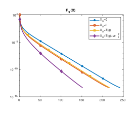
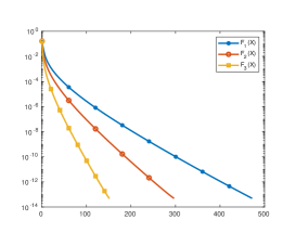
We show that, under mild assumptions, starting with X0=0subscript𝑋00X_{0}=0, the sequences generated by F1,F2,F3subscript𝐹1subscript𝐹2subscript𝐹3F_{1},F_{2},F_{3} converge monotonically and linearly to G𝐺G in the infinity norm. Moreover, we prove that the rate of convergence of the sequence generated by F3subscript𝐹3F_{3} is better than the rate of the sequence generated by F2subscript𝐹2F_{2}, which in turn is better than that generated by F1subscript𝐹1F_{1}. We prove that if X0subscript𝑋0X_{0} is row-stochastic then all the matrices Xksubscript𝑋𝑘X_{k} are row-stochastic and the rate of convergence of each of the three iterations is better than that obtained with X0=0subscript𝑋00X_{0}=0. Numerical experiments show also the evidence that for X0=T(g)subscript𝑋0𝑇𝑔X_{0}=T(g) the rate of convergence of the three sequences is even better.

Then we adapt Newton’s iteration, in the form given by [16], to the case of QT coefficients. In order to solve the Sylvester equation arising at each step of Newton’s iteration we rely on the solver introduced in [28]. Under mild conditions, we prove that, for X0=0subscript𝑋00X_{0}=0, convergence holds in the infinity norm, is monotonic and quadratic.

In order to evaluate an a posteriori bound on the approximation error in the computation of G𝐺G, we also perform the analysis of the structured condition number. More specifically, we provide perturbation results related to perturbations of the Toeplitz part and of the correction part in the matrix coefficients Aisubscript𝐴𝑖A_{i}, i=1,0,1𝑖101i=-1,0,1, and we estimate the consequent variation of the solution G𝐺G and of its Toeplitz part T(g)𝑇𝑔T(g).

Numerical experiments are reported which show the effectiveness of our approach and the reliability of our algorithms with respect to the algorithm CR. In particular we show that in certain cases the combination of Newton’s iteration and cyclic reduction provides a substantial acceleration of the convergence.

The paper is organized as follows: in Section 2 we recall some preliminary properties and concepts useful for the analysis of the problem; in Section 3 we present an algorithm for computing the Toeplitz part T(g)𝑇𝑔T(g) of the solution; Section 4 deals with the analysis of three fixed-point iterations applied to infinite QT matrices, while Section 5 concerns the algorithmic analysis of Newton iteration; in Section 6 we carry out the analysis of the conditioning by providing some perturbation results, while in Section 7 we present and discuss some numerical experiments which show the effectiveness of our approach.

2 Preliminaries

Let superscript\ell^{\infty} be the set of sequences x=(xi)i𝑥subscriptsubscript𝑥𝑖𝑖x=(x_{i})_{i\in\mathbb{N}} such that x:=supi|xi|assignsubscriptnorm𝑥subscriptsupremum𝑖subscript𝑥𝑖\|x\|_{\infty}:=\sup_{i}|x_{i}| is finite. Consider the set of matrices A=(ai,j)𝐴subscript𝑎𝑖𝑗A=(a_{i,j}) such that the application xy=Ax𝑥𝑦𝐴𝑥x\to y=Ax, where yj=j=1ai,jxjsubscript𝑦𝑗superscriptsubscript𝑗1subscript𝑎𝑖𝑗subscript𝑥𝑗y_{j}=\sum_{j=1}^{\infty}a_{i,j}x_{j}, defines a linear operator from superscript\ell^{\infty} to superscript\ell^{\infty}. Denote this set by subscript\mathcal{L}_{\infty} and define the induced norm A=supx=1Axsubscriptnorm𝐴subscriptsupremumsubscriptnorm𝑥1subscriptnorm𝐴𝑥\|A\|_{\infty}=\sup_{\|x\|_{\infty}=1}\|Ax\|_{\infty}. It can be verified that A=supij=1|ai,j|subscriptnorm𝐴subscriptsupremum𝑖superscriptsubscript𝑗1subscript𝑎𝑖𝑗\|A\|_{\infty}=\sup_{i}\sum_{j=1}^{\infty}|a_{i,j}|. Recall that subscript\mathcal{L}_{\infty} is a Banach algebra, that is, it is closed under the row-by-column product, the norm satisfies ABABsubscriptnorm𝐴𝐵subscriptnorm𝐴subscriptnorm𝐵\|AB\|_{\infty}\leq\|A\|_{\infty}\cdot\|B\|_{\infty} for any A,B𝐴𝐵subscriptA,B\in\mathcal{L}_{\infty}, and the normed space is complete.

We introduce the following notation

(4) ai(z)=ai,1z1+ai,0+ai,1zsubscript𝑎𝑖𝑧subscript𝑎𝑖1superscript𝑧1subscript𝑎𝑖0subscript𝑎𝑖1𝑧\displaystyle a_{i}(z)=a_{i,-1}z^{-1}+a_{i,0}+a_{i,1}z
bi(z)=bi,0+bi,1z,subscript𝑏𝑖𝑧subscript𝑏𝑖0subscript𝑏𝑖1𝑧\displaystyle b_{i}(z)=b_{i,0}+b_{i,1}z,

so that we may write Ai=T(ai)+Eisubscript𝐴𝑖𝑇subscript𝑎𝑖subscript𝐸𝑖A_{i}=T(a_{i})+E_{i}, for i=1,0,1𝑖101i=-1,0,1, where Eisubscript𝐸𝑖E_{i} has null entries except for those in the first row which are equal to [bi,0ai,0,bi,1ai,1,0,]subscript𝑏𝑖0subscript𝑎𝑖0subscript𝑏𝑖1subscript𝑎𝑖10[b_{i,0}-a_{i,0},b_{i,1}-a_{i,1},0,\ldots]. We assume that the entries of Aisubscript𝐴𝑖A_{i} are nonnegative and (A1+A0+A1)𝟏=𝟏subscript𝐴1subscript𝐴0subscript𝐴111(A_{-1}+A_{0}+A_{1}){\bm{1}}={\bm{1}}, where 𝟏1{\bm{1}} is the vector of all ones of appropriate dimension. It is known [19], [31] that under these conditions, there exist the minimal nonnegative solutions R𝑅R and G𝐺G of (1) and (2), respectively, and the Laurent matrix polynomial φ(z)=z1A1+A0I+zA1𝜑𝑧superscript𝑧1subscript𝐴1subscript𝐴0𝐼𝑧subscript𝐴1\varphi(z)=z^{-1}A_{-1}+A_{0}-I+zA_{1} admits the factorization

φ(z)=(IzR)W(Iz1G)𝜑𝑧𝐼𝑧𝑅𝑊𝐼superscript𝑧1𝐺\varphi(z)=-(I-zR)W(I-z^{-1}G)

where

(5) A1=RW,A1=WG,A0=IWRWG,formulae-sequencesubscript𝐴1𝑅𝑊formulae-sequencesubscript𝐴1𝑊𝐺subscript𝐴0𝐼𝑊𝑅𝑊𝐺\displaystyle A_{1}=RW,\quad A_{-1}=WG,\quad A_{0}=I-W-RWG,
W=IA0A1G=IA0RA1,𝑊𝐼subscript𝐴0subscript𝐴1𝐺𝐼subscript𝐴0𝑅subscript𝐴1\displaystyle W=I-A_{0}-A_{1}G=I-A_{0}-RA_{-1},
G𝟏𝟏.𝐺11\displaystyle G{\bm{1}}\leq{\bm{1}}.

Observe that if a1(1)=0subscript𝑎110a_{-1}(1)=0, i.e., A1=e1wTsubscript𝐴1subscript𝑒1superscript𝑤𝑇A_{-1}=e_{1}w^{T}, wT=(b1,0,b1,1,0,)0superscript𝑤𝑇subscript𝑏10subscript𝑏1100w^{T}=(b_{-1,0},b_{-1,1},0,\ldots)\neq 0, then the minimal nonnegative solution G𝐺G of equation (1) can be expressed in the form G=𝟏vT𝐺1superscript𝑣𝑇G={\bm{1}}v^{T} where v=1b1(1)w𝑣1subscript𝑏11𝑤v=\frac{1}{b_{-1}(1)}w. Therefore, without loss of generality we may assume that a1(1)>0subscript𝑎110a_{-1}(1)>0.

The following result is valid if a1(1)>0subscript𝑎110a_{-1}(1)>0 and b1(1)>0subscript𝑏110b_{-1}(1)>0, that is, A1𝟏>0subscript𝐴110A_{-1}{\bm{1}}>0.

Lemma 2.1.

Assume A1𝟏>0subscript𝐴110A_{-1}{\bm{1}}>0 and define

(6) θ=min{a1(1),b1(1)},γ=max{a1(1)a1(1),b1(1)b1(1)}.formulae-sequence𝜃subscript𝑎11subscript𝑏11𝛾subscript𝑎11subscript𝑎11subscript𝑏11subscript𝑏11\theta=\min\{a_{-1}(1),b_{-1}(1)\},\quad\gamma=\max\left\{\frac{a_{1}(1)}{a_{-1}(1)},\frac{b_{1}(1)}{b_{-1}(1)}\right\}.

Then the matrix W=IA0A1G𝑊𝐼subscript𝐴0subscript𝐴1𝐺W=I-A_{0}-A_{1}G is invertible in subscript\mathcal{L}_{\infty}, has nonnegative inverse, and W111(A0+A1)𝟏=1θsubscriptnormsuperscript𝑊111subscriptnormsubscript𝐴0subscript𝐴111𝜃\|W^{-1}\|_{\infty}\leq\frac{1}{1-\|(A_{0}+A_{1}){\bm{1}}\|_{\infty}}=\frac{1}{\theta}. Moreover, W1RWγsubscriptnormsuperscript𝑊1𝑅𝑊𝛾\|W^{-1}RW\|_{\infty}\leq\gamma. If A1𝟏>A1𝟏subscript𝐴11subscript𝐴11A_{-1}{\bm{1}}>A_{1}{\bm{1}} then γ<1𝛾1\gamma<1.

Proof 2.2.

Observe that A0+A1G=(A0+A1G)𝟏(A0+A1)𝟏=(IA1)𝟏=1θ<1subscriptnormsubscript𝐴0subscript𝐴1𝐺subscriptnormsubscript𝐴0subscript𝐴1𝐺1subscriptnormsubscript𝐴0subscript𝐴11subscriptnorm𝐼subscript𝐴111𝜃1\|A_{0}+A_{1}G\|_{\infty}=\|(A_{0}+A_{1}G){\bm{1}}\|_{\infty}\leq\|(A_{0}+A_{1}){\bm{1}}\|_{\infty}=\|(I-A_{-1}){\bm{1}}\|_{\infty}=1-\theta<1, since (A0+A1)𝟏=(IA1)𝟏subscript𝐴0subscript𝐴11𝐼subscript𝐴11(A_{0}+A_{1}){\bm{1}}=(I-A_{-1}){\bm{1}}, A1𝟏>0subscript𝐴110A_{-1}{\bm{1}}>0 and A1𝟏=(b1(1),a1(1),a1(1),)Tsubscript𝐴11superscriptsubscript𝑏11subscript𝑎11subscript𝑎11𝑇A_{-1}{\bm{1}}=(b_{-1}(1),a_{-1}(1),a_{-1}(1),\ldots)^{T}. Therefore W1superscript𝑊1subscriptW^{-1}\in\mathcal{L}_{\infty} and is nonnegative, being W1=i=0(A0+A1G)isuperscript𝑊1superscriptsubscript𝑖0superscriptsubscript𝐴0subscript𝐴1𝐺𝑖W^{-1}=\sum_{i=0}^{\infty}(A_{0}+A_{1}G)^{i} and

W1=k=0(A0+A1G)k𝟏11A0+A1=1θ.subscriptnormsuperscript𝑊1subscriptnormsuperscriptsubscript𝑘0superscriptsubscript𝐴0subscript𝐴1𝐺𝑘111subscriptnormsubscript𝐴0subscript𝐴11𝜃\|W^{-1}\|_{\infty}=\|\sum_{k=0}^{\infty}(A_{0}+A_{1}G)^{k}{\bm{1}}\|_{\infty}\leq\frac{1}{1-\|A_{0}+A_{1}\|_{\infty}}=\frac{1}{\theta}.

Now we show that W1RWγsubscriptnormsuperscript𝑊1𝑅𝑊𝛾\|W^{-1}RW\|_{\infty}\leq\gamma. Since W1RW=W1A1superscript𝑊1𝑅𝑊superscript𝑊1subscript𝐴1W^{-1}RW=W^{-1}A_{1} by (5), it is sufficient to consider W1A1=W1A1𝟏subscriptnormsuperscript𝑊1subscript𝐴1subscriptnormsuperscript𝑊1subscript𝐴11\|W^{-1}A_{1}\|_{\infty}=\|W^{-1}A_{1}{\bm{1}}\|_{\infty}. By definition of γ𝛾\gamma we have A1𝟏γA1𝟏subscript𝐴11𝛾subscript𝐴11A_{1}{\bm{1}}\leq\gamma A_{-1}{\bm{1}}, therefore

W1A1𝟏γW1A1𝟏=γG𝟏γ𝟏,superscript𝑊1subscript𝐴11𝛾superscript𝑊1subscript𝐴11𝛾𝐺1𝛾1W^{-1}A_{1}{\bm{1}}\leq\gamma W^{-1}A_{-1}{\bm{1}}=\gamma G{\bm{1}}\leq\gamma{\bm{1}},

where we used the fact that W1A1=Gsuperscript𝑊1subscript𝐴1𝐺W^{-1}A_{-1}=G. Thus we have W1RWγsubscriptnormsuperscript𝑊1𝑅𝑊𝛾\|W^{-1}RW\|_{\infty}\leq\gamma. Since A1𝟏=(b1(1),a1(1),a1(1),)Tsubscript𝐴11superscriptsubscript𝑏11subscript𝑎11subscript𝑎11𝑇A_{1}{\bm{1}}=(b_{1}(1),a_{1}(1),a_{1}(1),\ldots)^{T} and A1𝟏=(b1(1),a1(1),a1(1),)Tsubscript𝐴11superscriptsubscript𝑏11subscript𝑎11subscript𝑎11𝑇A_{-1}{\bm{1}}=(b_{-1}(1),a_{-1}(1),a_{-1}(1),\ldots)^{T} then A1𝟏>A1𝟏subscript𝐴11subscript𝐴11A_{-1}{\bm{1}}>A_{1}{\bm{1}} implies γ<1𝛾1\gamma<1.

Define 𝒲={f(z)=ifizi:fw:=i|fi|<}\mathcal{W}=\{f(z)=\sum_{i\in\mathbb{Z}}f_{i}z^{i}:\quad\|f\|_{w}:=\sum_{i\in\mathbb{Z}}|f_{i}|<\infty\}. Consider the following class

𝒬𝒯:={A=T(f)+E}assign𝒬𝒯𝐴𝑇𝑓𝐸\mathcal{QT}:=\{A=T(f)+E\}

where f(z)𝒲𝑓𝑧𝒲f(z)\in\mathcal{W}, the matrix E=(ei,j)𝐸subscript𝑒𝑖𝑗subscriptE=(e_{i,j})\in\mathcal{L}_{\infty} is such that limivi=0subscript𝑖subscript𝑣𝑖0\lim_{i}v_{i}=0, where vi=j=1|ei,j|subscript𝑣𝑖superscriptsubscript𝑗1subscript𝑒𝑖𝑗v_{i}=\sum_{j=1}^{\infty}|e_{i,j}|.

Observe that Ai𝒬𝒯subscript𝐴𝑖𝒬𝒯A_{i}\in\mathcal{QT} for i=1,0,1𝑖101i=-1,0,1, moreover, in [5] it is shown that 𝒬𝒯𝒬𝒯\mathcal{QT} is an algebra with the infinity norm, and the matrices W,G𝑊𝐺W,G and R𝑅R in (5) belong to 𝒬𝒯𝒬𝒯\mathcal{QT} if A1𝟏>A1𝟏subscript𝐴11subscript𝐴11A_{-1}{\bm{1}}>A_{1}{\bm{1}} or if A1𝟏A1𝟏>0subscript𝐴11subscript𝐴110A_{-1}{\bm{1}}\geq A_{1}{\bm{1}}>0. More precisely we have the following result

Theorem 2.3.

The minimal nonnegative solution G𝐺G of the matrix equation (1) can be written as G=T(g)+Eg𝐺𝑇𝑔subscript𝐸𝑔G=T(g)+E_{g} where g(z)=igizi𝒲𝑔𝑧subscript𝑖subscript𝑔𝑖superscript𝑧𝑖𝒲g(z)=\sum_{i\in\mathbb{Z}}g_{i}z^{i}\in\mathcal{W} is such that gi0subscript𝑔𝑖0g_{i}\geq 0 and gw=g(1)1subscriptnorm𝑔𝑤𝑔11\|g\|_{w}=g(1)\leq 1. Moreover, for any z𝑧z such that |z|=1𝑧1|z|=1, g(z)𝑔𝑧g(z) is a solution of minimum modulus of the quadratic equation

(7) a1(z)+a0(z)λ+a1(z)λ2=λ.subscript𝑎1𝑧subscript𝑎0𝑧𝜆subscript𝑎1𝑧superscript𝜆2𝜆\displaystyle a_{-1}(z)+a_{0}(z)\lambda+a_{1}(z)\lambda^{2}=\lambda.

This solution is unique if there exists j𝑗j such that ai,j0subscript𝑎𝑖𝑗0a_{i,j}\neq 0 for at least two different values of i𝑖i. If

A1𝟏>A1𝟏, or A1𝟏A1𝟏>0,formulae-sequencesubscript𝐴11subscript𝐴11 or subscript𝐴11subscript𝐴110A_{-1}{\bm{1}}>A_{1}{\bm{1}},\quad\hbox{ or }\quad A_{-1}{\bm{1}}\geq A_{1}{\bm{1}}>0,

then G𝒬𝒯𝐺𝒬𝒯G\in\mathcal{QT}, G𝟏=𝟏𝐺11G{\bm{1}}={\bm{1}} and g(1)=1𝑔11g(1)=1. Conversely, if G𝟏=𝟏𝐺11G{\bm{1}}={\bm{1}} and G𝒬𝒯𝐺𝒬𝒯G\in\mathcal{QT} then a1(1)a1(1)subscript𝑎11subscript𝑎11a_{-1}(1)\geq a_{1}(1) and g(1)=1𝑔11g(1)=1.

Observe that the condition

(8) A1𝟏>A1𝟏subscript𝐴11subscript𝐴11A_{-1}{\bm{1}}>A_{1}{\bm{1}}

is equivalent to a1(1)>a1(1)subscript𝑎11subscript𝑎11a_{-1}(1)>a_{1}(1) and b1(1)>b1(1)subscript𝑏11subscript𝑏11b_{-1}(1)>b_{1}(1). In the following we assume that (8) holds and that there exists i𝑖i such that ai,j0subscript𝑎𝑖𝑗0a_{i,j}\neq 0 for at least two values of j𝑗j. The latter condition is very mild.

3 Computing the symbol g(z)𝑔𝑧g(z)

Relying on Theorem 2.3, we provide an algorithm, based on the evaluation/interpolation at the roots of 1, for computing an approximation g^isubscript^𝑔𝑖\hat{g}_{i}, i=n+1,,n𝑖𝑛1𝑛i=-n+1,\ldots,n, to the coefficients gisubscript𝑔𝑖g_{i} of g(z)𝑔𝑧g(z), where n𝑛n is such that |g^igi|ϵ/(2n)subscript^𝑔𝑖subscript𝑔𝑖italic-ϵ2𝑛|\hat{g}_{i}-g_{i}|\leq\epsilon/(2n), for any i𝑖i and for a given tolerance ϵ>0italic-ϵ0\epsilon>0. In this analysis we may relax the assumption a1(1)>a1(1)subscript𝑎11subscript𝑎11a_{-1}(1)>a_{1}(1) so that the result holds in general.

Let n>0𝑛0n>0 be an integer and set m=2n𝑚2𝑛m=2n. Define ωm=cos2πm+𝐢sin2πmsubscript𝜔𝑚2𝜋𝑚𝐢2𝜋𝑚\omega_{m}=\cos\frac{2\pi}{m}+\mathbf{i}\sin\frac{2\pi}{m} a principal m𝑚mth root of 1, where 𝐢𝐢\mathbf{i} is the imaginary unit such that 𝐢2=1superscript𝐢21\mathbf{i}^{2}=-1. Rewrite g(z)𝑔𝑧g(z) as

(9) g(z)=j=n+1ngjzj+j=n+1nk1(zmk+jgmk+j+zmkj+1gmkj+1).𝑔𝑧superscriptsubscript𝑗𝑛1𝑛subscript𝑔𝑗superscript𝑧𝑗superscriptsubscript𝑗𝑛1𝑛subscript𝑘1superscript𝑧𝑚𝑘𝑗subscript𝑔𝑚𝑘𝑗superscript𝑧𝑚𝑘𝑗1subscript𝑔𝑚𝑘𝑗1g(z)=\sum_{j=-n+1}^{n}g_{j}z^{j}+\sum_{j=-n+1}^{n}\sum_{k\geq 1}(z^{mk+j}g_{mk+j}+z^{-mk-j+1}g_{-mk-j+1}).

Since ωmkm=1superscriptsubscript𝜔𝑚𝑘𝑚1\omega_{m}^{km}=1, from (9) we have

g(ωmi)=j=n+1ngjωmij+j=n+1n(ωmijk1gmk+j+ωmi(j1)k1gmkj+1).𝑔superscriptsubscript𝜔𝑚𝑖superscriptsubscript𝑗𝑛1𝑛subscript𝑔𝑗superscriptsubscript𝜔𝑚𝑖𝑗superscriptsubscript𝑗𝑛1𝑛superscriptsubscript𝜔𝑚𝑖𝑗subscript𝑘1subscript𝑔𝑚𝑘𝑗superscriptsubscript𝜔𝑚𝑖𝑗1subscript𝑘1subscript𝑔𝑚𝑘𝑗1g(\omega_{m}^{i})=\sum_{j=-n+1}^{n}g_{j}\omega_{m}^{ij}+\sum_{j=-n+1}^{n}(\omega_{m}^{ij}\sum_{k\geq 1}g_{mk+j}+\omega_{m}^{-i(j-1)}\sum_{k\geq 1}g_{-mk-j+1}).

Therefore, the Laurent polynomial defined by

(10) g^(z)=j=n+1ngjzj+j=n+1n(zjg^j++zj+1g^j+1),^𝑔𝑧superscriptsubscript𝑗𝑛1𝑛subscript𝑔𝑗superscript𝑧𝑗superscriptsubscript𝑗𝑛1𝑛superscript𝑧𝑗superscriptsubscript^𝑔𝑗superscript𝑧𝑗1superscriptsubscript^𝑔𝑗1\displaystyle\widehat{g}(z)=\sum_{j=-n+1}^{n}g_{j}z^{j}+\sum_{j=-n+1}^{n}(z^{j}\hat{g}_{j}^{+}+z^{-j+1}\hat{g}_{-j+1}^{-}),
g^j+=k1gmk+j,g^j+1=k1gmkj+1,j=n+1,,n,formulae-sequencesuperscriptsubscript^𝑔𝑗subscript𝑘1subscript𝑔𝑚𝑘𝑗formulae-sequencesuperscriptsubscript^𝑔𝑗1subscript𝑘1subscript𝑔𝑚𝑘𝑗1𝑗𝑛1𝑛\displaystyle\hat{g}_{j}^{+}=\sum_{k\geq 1}g_{mk+j},\quad\hat{g}_{-j+1}^{-}=\sum_{k\geq 1}g_{-mk-j+1},~{}~{}j=-n+1,\ldots,n,

is such that g(ωmi)=g^(ωmi)𝑔superscriptsubscript𝜔𝑚𝑖^𝑔superscriptsubscript𝜔𝑚𝑖g(\omega_{m}^{i})=\hat{g}(\omega_{m}^{i}), that is, it interpolates g(z)𝑔𝑧g(z) at the m𝑚m-th roots of 1.

The following lemma provides a bound to the tail of the Laurent series g(z)𝑔𝑧g(z) and extends to the case of Laurent series a similar property proved in [8] valid for power series.

Lemma 3.1.

Let g(z)𝑔𝑧g(z) be the solution of minimum modulus of equation (7). Let g^(z)=j=n+1ng^jzj^𝑔𝑧superscriptsubscript𝑗𝑛1𝑛subscript^𝑔𝑗superscript𝑧𝑗\hat{g}(z)=\sum_{j=-n+1}^{n}\hat{g}_{j}z^{j} be the Laurent polynomial interpolating g(z)𝑔𝑧g(z) at the m𝑚m-th roots of 1, i.e., such that g(ωmi)=g^(ωmi)𝑔superscriptsubscript𝜔𝑚𝑖^𝑔superscriptsubscript𝜔𝑚𝑖g(\omega_{m}^{i})=\hat{g}(\omega_{m}^{i}), i=n+1,,n𝑖𝑛1𝑛i=-n+1,\ldots,n, where m=2n𝑚2𝑛m=2n. If g′′(x)𝒲superscript𝑔′′𝑥𝒲g^{\prime\prime}(x)\in\mathcal{W}, then g′′(1)0superscript𝑔′′10g^{\prime\prime}(1)\geq 0 and

(11) g′′(1)g^′′(1)2n(j<n+1gj+j>ngj),superscript𝑔′′1superscript^𝑔′′12𝑛subscript𝑗𝑛1subscript𝑔𝑗subscript𝑗𝑛subscript𝑔𝑗g^{\prime\prime}(1)-\hat{g}^{\prime\prime}(1)\geq 2n\left(\sum_{j<-n+1}g_{j}+\sum_{j>n}g_{j}\right),

moreover 0g^jgj12n(g′′(1)g^′′(1))0subscript^𝑔𝑗subscript𝑔𝑗12𝑛superscript𝑔′′1superscript^𝑔′′10\leq\hat{g}_{j}-g_{j}\leq\frac{1}{2n}(g^{\prime\prime}(1)-\hat{g}^{\prime\prime}(1)), for j=n+1,,n𝑗𝑛1𝑛j=-n+1,\ldots,n.

Proof 3.2.

Since the coefficients gisubscript𝑔𝑖g_{i} are nonnegative then also g′′(z)superscript𝑔′′𝑧g^{\prime\prime}(z) has nonnegative coefficients, moreover, since g′′(z)𝒲superscript𝑔′′𝑧𝒲g^{\prime\prime}(z)\in\mathcal{W}, then the series g′′(1)superscript𝑔′′1g^{\prime\prime}(1) is absolutely convergent and g′′(1)0superscript𝑔′′10g^{\prime\prime}(1)\geq 0. Thus, from the representation (9), in view of (10), we deduce that

g′′(1)g^′′(1)=j=n+1nk1(gmk+jαj,k+gmkj+1αj,k),superscript𝑔′′1superscript^𝑔′′1superscriptsubscript𝑗𝑛1𝑛subscript𝑘1subscript𝑔𝑚𝑘𝑗subscript𝛼𝑗𝑘subscript𝑔𝑚𝑘𝑗1subscript𝛼𝑗𝑘g^{\prime\prime}(1)-\hat{g}^{\prime\prime}(1)=\sum_{j=-n+1}^{n}\sum_{k\geq 1}\left(g_{mk+j}\alpha_{j,k}+g_{-mk-j+1}\alpha_{j,k}\right),

where αj,k=(mk+j)(mk+j1)j(j1)subscript𝛼𝑗𝑘𝑚𝑘𝑗𝑚𝑘𝑗1𝑗𝑗1\alpha_{j,k}=(mk+j)(mk+j-1)-j(j-1). The inequality (11) follows from the nonnegativity of the coefficients and from the property αj,kmsubscript𝛼𝑗𝑘𝑚\alpha_{j,k}\geq m, valid for k1,j=n+1,,nformulae-sequence𝑘1𝑗𝑛1𝑛k\geq 1,~{}j=-n+1,\ldots,n which can be verified by a direct inspection. The bound on g^jgjsubscript^𝑔𝑗subscript𝑔𝑗\hat{g}_{j}-g_{j} follows from (11) since g^j=gj+g^j++g^jsubscript^𝑔𝑗subscript𝑔𝑗superscriptsubscript^𝑔𝑗superscriptsubscript^𝑔𝑗\hat{g}_{j}=g_{j}+\hat{g}_{j}^{+}+\hat{g}_{j}^{-} and g^j++g^jj<n+1gj+j>ngjsubscriptsuperscript^𝑔𝑗superscriptsubscript^𝑔𝑗subscript𝑗𝑛1subscript𝑔𝑗subscript𝑗𝑛subscript𝑔𝑗\hat{g}^{+}_{j}+\hat{g}_{j}^{-}\leq\sum_{j<-n+1}g_{j}+\sum_{j>n}g_{j} in view of (10).

Observe that g^′′(1)superscript^𝑔′′1\hat{g}^{\prime\prime}(1) is computable once the coefficients of the polynomial g^(z)^𝑔𝑧\hat{g}(z) have been computed. Moreover, the value of g′′(1)superscript𝑔′′1g^{\prime\prime}(1) is computable even though g(z)𝑔𝑧g(z) is not known. In fact, by taking the second derivative in the equation obtained by replacing λ𝜆\lambda with g(z)𝑔𝑧g(z) in (7), i.e.,

a1(z)g(z)2+(a0(z)1)g(z)+a1(z)=0,subscript𝑎1𝑧𝑔superscript𝑧2subscript𝑎0𝑧1𝑔𝑧subscript𝑎1𝑧0a_{1}(z)g(z)^{2}+(a_{0}(z)-1)g(z)+a_{-1}(z)=0,

for z=1𝑧1z=1, the value of g′′(1)superscript𝑔′′1g^{\prime\prime}(1) can be easily expressed in terms of ai(1)subscript𝑎𝑖1a_{i}(1), ai(1)superscriptsubscript𝑎𝑖1a_{i}^{\prime}(1) and ai′′(1)superscriptsubscript𝑎𝑖′′1a_{i}^{\prime\prime}(1). More precisely, by taking the first derivative we obtain

a1(z)g(z)2+2g(z)g(z)a1(z)+(a0(z)1)g(z)+a0(z)g(z)+a1(z)=0,superscriptsubscript𝑎1𝑧𝑔superscript𝑧22𝑔𝑧superscript𝑔𝑧subscript𝑎1𝑧subscript𝑎0𝑧1superscript𝑔𝑧superscriptsubscript𝑎0𝑧𝑔𝑧superscriptsubscript𝑎1𝑧0a_{1}^{\prime}(z)g(z)^{2}+2g(z)g^{\prime}(z)a_{1}(z)+(a_{0}(z)-1)g^{\prime}(z)+a_{0}^{\prime}(z)g(z)+a_{-1}^{\prime}(z)=0,

which yields

(12) g(1)=a1(1)g(1)2+a0(1)g(1)+a1(1)12a1(1)g(1)a0(1),g(1)=min(1,a1(1)/a1(1)).formulae-sequencesuperscript𝑔1superscriptsubscript𝑎11𝑔superscript12superscriptsubscript𝑎01𝑔1superscriptsubscript𝑎1112subscript𝑎11𝑔1subscript𝑎01𝑔11subscript𝑎11subscript𝑎11g^{\prime}(1)=\frac{a_{1}^{\prime}(1)g(1)^{2}+a_{0}^{\prime}(1)g(1)+a_{-1}^{\prime}(1)}{1-2a_{1}(1)g(1)-a_{0}(1)},\quad g(1)=\min(1,a_{-1}(1)/a_{1}(1)).

By taking the second derivative for z=1𝑧1z=1, we get

a1′′(1)g(1)2+limit-fromsuperscriptsubscript𝑎1′′1𝑔superscript12\displaystyle a_{1}^{\prime\prime}(1)g(1)^{2}+ 2a1(1)g(1)g(1)+2a1(1)g(1)g(1)+2a1(1)g(1)22superscriptsubscript𝑎11superscript𝑔1𝑔12superscriptsubscript𝑎11superscript𝑔1𝑔12subscript𝑎11superscript𝑔superscript12\displaystyle 2a_{1}^{\prime}(1)g^{\prime}(1)g(1)+2a_{1}^{\prime}(1)g^{\prime}(1)g(1)+2a_{1}(1)g^{\prime}(1)^{2}
+\displaystyle+ 2a1(1)g′′(1)g(1)+(a0(1)1)g′′(1)+a0(1)g(1)2subscript𝑎11superscript𝑔′′1𝑔1subscript𝑎011superscript𝑔′′1superscriptsubscript𝑎01superscript𝑔1\displaystyle 2a_{1}(1)g^{\prime\prime}(1)g(1)+(a_{0}(1)-1)g^{\prime\prime}(1)+a_{0}^{\prime}(1)g^{\prime}(1)
+\displaystyle+ a0′′(1)g(1)+a0(1)g(1)+a1′′(1)=0superscriptsubscript𝑎0′′1𝑔1superscriptsubscript𝑎01superscript𝑔1superscriptsubscript𝑎1′′10\displaystyle a_{0}^{\prime\prime}(1)g(1)+a_{0}^{\prime}(1)g^{\prime}(1)+a_{-1}^{\prime\prime}(1)=0

which yields

(13) g′′(1)=superscript𝑔′′1absent\displaystyle g^{\prime\prime}(1)= [a1′′(1)+a0′′(1)g(1)+a1′′(1)g(1)2+2a1(1)g(1)2\displaystyle\left[a_{-1}^{\prime\prime}(1)+a_{0}^{\prime\prime}(1)g(1)+a_{1}^{\prime\prime}(1)g(1)^{2}+2a_{1}(1)g^{\prime}(1)^{2}\right.
+\displaystyle+ 2g(1)(2g(1)a1(1)+a0(1))]/(12a1(1)g(1)a0(1)).\displaystyle\left.2g^{\prime}(1)(2g(1)a_{1}^{\prime}(1)+a_{0}^{\prime}(1))\right]/(1-2a_{1}(1)g(1)-a_{0}(1)).

Lemma 3.1 provides an a posteriori bound to the error in the approximation of the Laurent series g(z)𝑔𝑧g(z) together with a stop condition for the following evaluation interpolation algorithm for computing the coefficients of g(z)𝑔𝑧g(z).

Algorithm 1 Approximation of g(z)𝑔𝑧g(z)
0:  The coefficients of ai(z)subscript𝑎𝑖𝑧a_{i}(z), i=1,0,1𝑖101i=-1,0,1 and a tolerance ϵ>0italic-ϵ0\epsilon>0.
0:  Approximations g^isubscript^𝑔𝑖\hat{g}_{i}, i=n+1,,n𝑖𝑛1𝑛i=-n+1,\ldots,n, to the coefficients gisubscript𝑔𝑖g_{i} of g(z)𝑔𝑧g(z) such that g^igiϵ/(2n)subscript^𝑔𝑖subscript𝑔𝑖italic-ϵ2𝑛\hat{g}_{i}-g_{i}\leq\epsilon/(2n).
1:  Set n=4𝑛4n=4, and compute g(1)=min(1,a1(1)/a1(1))𝑔11subscript𝑎11subscript𝑎11g(1)=\min(1,a_{-1}(1)/a_{1}(1)), g(1)superscript𝑔1g^{\prime}(1) and g′′(1)superscript𝑔′′1g^{\prime\prime}(1) by means of (12) and (13);
2:  Set m=2n𝑚2𝑛m=2n, ωm=cos2πm+𝐢sin2πmsubscript𝜔𝑚2𝜋𝑚𝐢2𝜋𝑚\omega_{m}=\cos\frac{2\pi}{m}+\mathbf{i}\sin\frac{2\pi}{m}, and evaluate a1(z),a0(z),a1(z)subscript𝑎1𝑧subscript𝑎0𝑧subscript𝑎1𝑧a_{-1}(z),~{}a_{0}(z),~{}a_{1}(z) at z=ωmi𝑧subscriptsuperscript𝜔𝑖𝑚z=\omega^{i}_{m}, i=n+1,,n𝑖𝑛1𝑛i=-n+1,\ldots,n;
3:  For i=n+1,,n𝑖𝑛1𝑛i=-n+1,\ldots,n, compute the solution λisubscript𝜆𝑖\lambda_{i} of minimum modulus of the quadratic equation (7), where z=ωmi𝑧superscriptsubscript𝜔𝑚𝑖z=\omega_{m}^{i};
4:  Interpolate the values λisubscript𝜆𝑖\lambda_{i}, i=n+1,,n𝑖𝑛1𝑛i=-n+1,\ldots,n by means of FFT and obtain the coefficients g^isubscript^𝑔𝑖\hat{g}_{i} of the Laurent polynomial g^(z)=i=n+1ng^izi^𝑔𝑧superscriptsubscript𝑖𝑛1𝑛subscript^𝑔𝑖superscript𝑧𝑖\hat{g}(z)=\sum_{i=-n+1}^{n}\hat{g}_{i}z^{i} such that g(ωmi)=g^(ωmi)𝑔superscriptsubscript𝜔𝑚𝑖^𝑔superscriptsubscript𝜔𝑚𝑖g(\omega_{m}^{i})=\hat{g}(\omega_{m}^{i}), i=n+1,,n𝑖𝑛1𝑛i=-n+1,\ldots,n;
5:  Compute δm=g′′(1)g^′′(1)subscript𝛿𝑚superscript𝑔′′1superscript^𝑔′′1\delta_{m}=g^{\prime\prime}(1)-\hat{g}^{\prime\prime}(1), where g^′′(1)=i=n+1ni(i1)g^isuperscript^𝑔′′1superscriptsubscript𝑖𝑛1𝑛𝑖𝑖1subscript^𝑔𝑖\hat{g}^{\prime\prime}(1)=\sum_{i=-n+1}^{n}i(i-1)\hat{g}_{i};
6:  If δm/mϵsubscript𝛿𝑚𝑚italic-ϵ\delta_{m}/m\leq\epsilon then exit, else set n=2n𝑛2𝑛n=2n and continue from Step 2.

Observe that the error bound converges to zero at least as O(1/n)𝑂1𝑛O(1/n). If the function g(z)𝑔𝑧g(z) is analytic in a neighborhood of the unit circle, then its coefficients decay exponentially to zero [12] so that also the the bound on the error converges exponentially to zero. It is also interesting to observe that, for n𝑛n\to\infty, the convergence of the coefficients of g^(z)^𝑔𝑧\hat{g}(z) to the corresponding coefficients of g(z)𝑔𝑧g(z) is monotonic.

Finally observe that the overall computational cost of this algorithm is O(nlogn)𝑂𝑛𝑛O(n\log n) arithmetic operations. In order to complete the computation of G𝐺G it remains to approximate the correction Egsubscript𝐸𝑔E_{g}. In view of the fact that Egsubscript𝐸𝑔E_{g} has entries ei,j(g)subscriptsuperscript𝑒𝑔𝑖𝑗e^{(g)}_{i,j} such that vi=j|ei,j(g)|subscript𝑣𝑖subscript𝑗subscriptsuperscript𝑒𝑔𝑖𝑗v_{i}=\sum_{j}|e^{(g)}_{i,j}| is finite and limivi=0subscript𝑖subscript𝑣𝑖0\lim_{i}v_{i}=0, we can approximate Egsubscript𝐸𝑔E_{g} with a finite number of parameter within an error bound ϵitalic-ϵ\epsilon. This computation is performed by means of functional iteration and is analyzed in the next section.

4 Fixed point iterations

In this section we analyze the convergence of sequences generated by a functional iteration of the kind Xk+1=F(Xk)subscript𝑋𝑘1𝐹subscript𝑋𝑘X_{k+1}=F(X_{k}), k=0,1,𝑘01k=0,1,\ldots, where F(X)𝐹𝑋F(X) is a matrix function such that G=F(G)𝐺𝐹𝐺G=F(G) where G𝐺G is the minimal nonnegative solution of (1). More precisely, we will consider the following cases

(14) F1(X)=A1+A0X+A1X2,subscript𝐹1𝑋subscript𝐴1subscript𝐴0𝑋subscript𝐴1superscript𝑋2\displaystyle F_{1}(X)=A_{-1}+A_{0}X+A_{1}X^{2},
F2(X)=(IA0)1(A1+A1X2),subscript𝐹2𝑋superscript𝐼subscript𝐴01subscript𝐴1subscript𝐴1superscript𝑋2\displaystyle F_{2}(X)=(I-A_{0})^{-1}(A_{-1}+A_{1}X^{2}),
F3(X)=(IA0A1X)1A1,subscript𝐹3𝑋superscript𝐼subscript𝐴0subscript𝐴1𝑋1subscript𝐴1\displaystyle F_{3}(X)=(I-A_{0}-A_{1}X)^{-1}A_{-1},

while Newton iteration is considered in the next section.

In the case where A1,A0,A1subscript𝐴1subscript𝐴0subscript𝐴1A_{-1},A_{0},A_{1} are finite matrices, the convergence analysis of the sequences generated by the functions (14) has been performed in [21]. Here, we extend the results of [21] to the case of matrices of infinite size belonging to subscript\mathcal{L}_{\infty}. We need the following

Lemma 4.1.

Let A1𝟏>A1𝟏subscript𝐴11subscript𝐴11A_{-1}{\bm{1}}>A_{1}{\bm{1}}, and

(15) σ=1min(a1(1)a1(1),b1(1)b1(1))<1.𝜎1subscript𝑎11subscript𝑎11subscript𝑏11subscript𝑏111\sigma=1-\min(a_{-1}(1)-a_{1}(1),b_{-1}(1)-b_{1}(1))<1.

Let H1=A0+A1+A1Gsubscript𝐻1subscript𝐴0subscript𝐴1subscript𝐴1𝐺H_{1}=A_{0}+A_{1}+A_{1}G. Then H1σsubscriptnormsubscript𝐻1𝜎\|H_{1}\|_{\infty}\leq\sigma, so that A0σsubscriptnormsubscript𝐴0𝜎\|A_{0}\|_{\infty}\leq\sigma, A0+A1Gσsubscriptnormsubscript𝐴0subscript𝐴1𝐺𝜎\|A_{0}+A_{1}G\|_{\infty}\leq\sigma. Therefore IA0𝐼subscript𝐴0I-A_{0} and IA0A1G𝐼subscript𝐴0subscript𝐴1𝐺I-A_{0}-A_{1}G are invertible and, for H2=(IA0)1(A1+A1G)subscript𝐻2superscript𝐼subscript𝐴01subscript𝐴1subscript𝐴1𝐺H_{2}=(I-A_{0})^{-1}(A_{1}+A_{1}G), H3=(IA0A1G)1A1subscript𝐻3superscript𝐼subscript𝐴0subscript𝐴1𝐺1subscript𝐴1H_{3}=(I-A_{0}-A_{1}G)^{-1}A_{1} we have

H3H2H1σ<1.subscriptnormsubscript𝐻3subscriptnormsubscript𝐻2subscriptnormsubscript𝐻1𝜎1\|H_{3}\|_{\infty}\leq\|H_{2}\|_{\infty}\leq\|H_{1}\|_{\infty}\leq\sigma<1.

Proof 4.2.

We have A0+A1+A1G=(A0+A1+A1G)𝟏subscriptnormsubscript𝐴0subscript𝐴1subscript𝐴1𝐺subscriptnormsubscript𝐴0subscript𝐴1subscript𝐴1𝐺1\|A_{0}+A_{1}+A_{1}G\|_{\infty}=\|(A_{0}+A_{1}+A_{1}G){\bm{1}}\|_{\infty}. Moreover, since by Theorem 2.3 we have G𝟏=𝟏𝐺11G{\bm{1}}={\bm{1}} and 𝟏=(A1+A0+A1)𝟏1subscript𝐴1subscript𝐴0subscript𝐴11{\bm{1}}=(A_{-1}+A_{0}+A_{1}){\bm{1}}, then (A0+A1+A1G)𝟏=(A0+A1+A1)𝟏=𝟏(A1A1)𝟏σ𝟏subscript𝐴0subscript𝐴1subscript𝐴1𝐺1subscript𝐴0subscript𝐴1subscript𝐴111subscript𝐴1subscript𝐴11𝜎1(A_{0}+A_{1}+A_{1}G){\bm{1}}=(A_{0}+A_{1}+A_{1}){\bm{1}}={\bm{1}}-(A_{-1}-A_{1}){\bm{1}}\leq\sigma{\bm{1}}, by definition of σ𝜎\sigma. This implies A0+A1+A1Gσsubscriptnormsubscript𝐴0subscript𝐴1subscript𝐴1𝐺𝜎\|A_{0}+A_{1}+A_{1}G\|_{\infty}\leq\sigma. Since A0,A1,Gsubscript𝐴0subscript𝐴1𝐺A_{0},A_{1},G are nonnegative then A0A0+A1+A1Gσsubscriptnormsubscript𝐴0subscriptnormsubscript𝐴0subscript𝐴1subscript𝐴1𝐺𝜎\|A_{0}\|_{\infty}\leq\|A_{0}+A_{1}+A_{1}G\|_{\infty}\leq\sigma and A0+A1Gσsubscriptnormsubscript𝐴0subscript𝐴1𝐺𝜎\|A_{0}+A_{1}G\|_{\infty}\leq\sigma. The matrices IA0𝐼subscript𝐴0I-A_{0} and IA0A1G𝐼subscript𝐴0subscript𝐴1𝐺I-A_{0}-A_{1}G are invertible in subscript\mathcal{L}_{\infty} since, in general, if IB𝐼𝐵subscriptI-B\in\mathcal{L}_{\infty} is such that B<1subscriptnorm𝐵1\|B\|_{\infty}<1 then the series i=0Bisuperscriptsubscript𝑖0superscript𝐵𝑖\sum_{i=0}^{\infty}B^{i} has norm bounded by 1/(1B)11subscriptnorm𝐵1/(1-\|B\|_{\infty}) and coincides with (IB)1superscript𝐼𝐵1(I-B)^{-1}. Concerning H2subscript𝐻2H_{2} we have H2=H2𝟏subscriptnormsubscript𝐻2subscriptnormsubscript𝐻21\|H_{2}\|_{\infty}=\|H_{2}{\bm{1}}\|_{\infty}. Moreover,

H2𝟏subscript𝐻21\displaystyle H_{2}{\bm{1}} =(IA0)1(A1+A1G)𝟏=(IA0)1(IA0(A1A1G))𝟏absentsuperscript𝐼subscript𝐴01subscript𝐴1subscript𝐴1𝐺1superscript𝐼subscript𝐴01𝐼subscript𝐴0subscript𝐴1subscript𝐴1𝐺1\displaystyle=(I-A_{0})^{-1}(A_{1}+A_{1}G){\bm{1}}=(I-A_{0})^{-1}(I-A_{0}-(A_{-1}-A_{1}G)){\bm{1}}
=𝟏(IA0)1(A1A1G)𝟏𝟏(A1A1G)𝟏absent1superscript𝐼subscript𝐴01subscript𝐴1subscript𝐴1𝐺11subscript𝐴1subscript𝐴1𝐺1\displaystyle={\bm{1}}-(I-A_{0})^{-1}(A_{-1}-A_{1}G){\bm{1}}\leq{\bm{1}}-(A_{-1}-A_{1}G){\bm{1}}
=(A0+A1+A1G)𝟏=H1𝟏,absentsubscript𝐴0subscript𝐴1subscript𝐴1𝐺1subscript𝐻11\displaystyle=(A_{0}+A_{1}+A_{1}G){\bm{1}}=H_{1}{\bm{1}},

where we used the properties (A1A1G)𝟏>0subscript𝐴1subscript𝐴1𝐺10(A_{-1}-A_{1}G){\bm{1}}>0 and (IA0)1Isuperscript𝐼subscript𝐴01𝐼(I-A_{0})^{-1}\geq I. Concerning H3subscript𝐻3H_{3}, since A1𝟏=(IA0A1)𝟏=(IA0A1G(A1A1G))𝟏subscript𝐴11𝐼subscript𝐴0subscript𝐴11𝐼subscript𝐴0subscript𝐴1𝐺subscript𝐴1subscript𝐴1𝐺1A_{1}{\bm{1}}=(I-A_{0}-A_{-1}){\bm{1}}=(I-A_{0}-A_{1}G-(A_{-1}-A_{1}G)){\bm{1}} we have

H3𝟏subscript𝐻31\displaystyle H_{3}{\bm{1}} =(IA0A1G)1A1𝟏=𝟏(IA0A1G)1(A1A1G)𝟏absentsuperscript𝐼subscript𝐴0subscript𝐴1𝐺1subscript𝐴111superscript𝐼subscript𝐴0subscript𝐴1𝐺1subscript𝐴1subscript𝐴1𝐺1\displaystyle=(I-A_{0}-A_{1}G)^{-1}A_{1}{\bm{1}}={\bm{1}}-(I-A_{0}-A_{1}G)^{-1}(A_{-1}-A_{1}G){\bm{1}}
𝟏(IA0)1(A1A1G)𝟏=H2𝟏,absent1superscript𝐼subscript𝐴01subscript𝐴1subscript𝐴1𝐺1subscript𝐻21\displaystyle\leq{\bm{1}}-(I-A_{0})^{-1}(A_{-1}-A_{1}G){\bm{1}}=H_{2}{\bm{1}},

where we used the fact that G𝟏=𝟏𝐺11G{\bm{1}}={\bm{1}}, (A1A1G)𝟏>0subscript𝐴1subscript𝐴1𝐺10(A_{-1}-A_{1}G){\bm{1}}>0 and (IA0A1G)1(IA0)1superscript𝐼subscript𝐴0subscript𝐴1𝐺1superscript𝐼subscript𝐴01(I-A_{0}-A_{1}G)^{-1}\geq(I-A_{0})^{-1}.

Observe that, from Lemma 2.1 and from (5), it follows that H3=W1RWsubscript𝐻3superscript𝑊1𝑅𝑊H_{3}=W^{-1}RW and H3=W1RWγsubscriptnormsubscript𝐻3subscriptnormsuperscript𝑊1𝑅𝑊𝛾\|H_{3}\|_{\infty}=\|W^{-1}RW\|_{\infty}\leq\gamma where γ<1𝛾1\gamma<1 is defined in (6). This provides a different bound on the norm of H3subscript𝐻3H_{3}. Therefore we have

(16) H3τ,τ=min{γ,σ},formulae-sequencesubscriptnormsubscript𝐻3𝜏𝜏𝛾𝜎\|H_{3}\|_{\infty}\leq\tau,\quad\tau=\min\{\gamma,\sigma\},

with γ𝛾\gamma and σ𝜎\sigma defined in (6) and (15), respectively.

We are ready to prove the following result which shows that the three sequences generated by (14) starting with X0=0subscript𝑋00X_{0}=0 monotonically converge to G𝐺G, convergence holds in the infinity norm and is linear. Moreover, the convergence of the third iteration is faster than that of the second one, while the convergence of the second iteration is faster than that of the first one.

Theorem 4.3.

Assume that A1𝟏>A1𝟏subscript𝐴11subscript𝐴11A_{-1}{\bm{1}}>A_{1}{\bm{1}}. For i{1,2,3}𝑖123i\in\{1,2,3\} define Xk+1(i)=Fi(Xk(i))superscriptsubscript𝑋𝑘1𝑖subscript𝐹𝑖superscriptsubscript𝑋𝑘𝑖X_{k+1}^{(i)}=F_{i}(X_{k}^{(i)}), k=0,1,2,𝑘012k=0,1,2,\ldots, where X0(i)=0superscriptsubscript𝑋0𝑖0X_{0}^{(i)}=0 and Fi(X)subscript𝐹𝑖𝑋F_{i}(X) are given in (14). Then

  1. 1.

    the three sequences {Xk(i)}superscriptsubscript𝑋𝑘𝑖\{X_{k}^{(i)}\} are well defined,

  2. 2.

    0Xk(i)Xk+1(i)G0superscriptsubscript𝑋𝑘𝑖superscriptsubscript𝑋𝑘1𝑖𝐺0\leq X_{k}^{(i)}\leq X_{k+1}^{(i)}\leq G,

  3. 3.

    for the error k(i)=GXk(i)superscriptsubscript𝑘𝑖𝐺superscriptsubscript𝑋𝑘𝑖\mathcal{E}_{k}^{(i)}=G-X_{k}^{(i)} we have k+1(i)Hik(i)subscriptnormsuperscriptsubscript𝑘1𝑖subscriptnormsubscript𝐻𝑖subscriptnormsuperscriptsubscript𝑘𝑖\|\mathcal{E}_{k+1}^{(i)}\|_{\infty}\leq\|H_{i}\|_{\infty}\|\mathcal{E}_{k}^{(i)}\|_{\infty}, where Hisubscript𝐻𝑖H_{i}, i=1,2,3𝑖123i=1,2,3 are the matrices defined in Lemma 4.1, so that limkk(i)=0subscript𝑘subscriptnormsuperscriptsubscript𝑘𝑖0\lim_{k\to\infty}\|\mathcal{E}_{k}^{(i)}\|_{\infty}=0.

Proof 4.4.

The first iteration is clearly well defined. The second is well defined since, according to Lemma 4.1, the matrix IA0𝐼subscript𝐴0I-A_{0} is invertible in subscript\mathcal{L}_{\infty}. The third iteration is well defined as long as the matrix IA0A1Xk𝐼subscript𝐴0subscript𝐴1subscript𝑋𝑘I-A_{0}-A_{1}X_{k} is invertible. On the other hand if 0XkG0subscript𝑋𝑘𝐺0\leq X_{k}\leq G, the latter matrix is invertible in view of Lemma 4.1 since A0+A1XkA0+A1Gsubscriptnormsubscript𝐴0subscript𝐴1subscript𝑋𝑘subscriptnormsubscript𝐴0subscript𝐴1𝐺\|A_{0}+A_{1}X_{k}\|_{\infty}\leq\|A_{0}+A_{1}G\|_{\infty}. In order to prove that 0Xk(i)Xk+1(i)G0superscriptsubscript𝑋𝑘𝑖superscriptsubscript𝑋𝑘1𝑖𝐺0\leq X_{k}^{(i)}\leq X_{k+1}^{(i)}\leq G we use an induction argument. We prove it for the first iteration, i.e., for i=1𝑖1i=1, the same technique can be used for the other iterations. For notational simplicity we omit the superscript and write Xksubscript𝑋𝑘X_{k} in place of Xk(1)superscriptsubscript𝑋𝑘1X_{k}^{(1)}. Since for X0=0subscript𝑋00X_{0}=0 we have X1=A1subscript𝑋1subscript𝐴1X_{1}=A_{-1}, so that 0X0X10subscript𝑋0subscript𝑋10\leq X_{0}\leq X_{1} and GX1=GA1=(A0+A1G)G0𝐺subscript𝑋1𝐺subscript𝐴1subscript𝐴0subscript𝐴1𝐺𝐺0G-X_{1}=G-A_{-1}=(A_{0}+A_{1}G)G\geq 0. For the inductive step, assume that 0Xk1XkG0subscript𝑋𝑘1subscript𝑋𝑘𝐺0\leq X_{k-1}\leq X_{k}\leq G. We first show that 0XkXk+10subscript𝑋𝑘subscript𝑋𝑘10\leq X_{k}\leq X_{k+1}. From Xk+1=A1Xk2+A0Xk+A1subscript𝑋𝑘1subscript𝐴1superscriptsubscript𝑋𝑘2subscript𝐴0subscript𝑋𝑘subscript𝐴1X_{k+1}=A_{1}X_{k}^{2}+A_{0}X_{k}+A_{-1} and from the property 0Xk1Xk0subscript𝑋𝑘1subscript𝑋𝑘0\leq X_{k-1}\leq X_{k} we get

Xk+1A1Xk12+A0Xk1+A1=Xk.subscript𝑋𝑘1subscript𝐴1superscriptsubscript𝑋𝑘12subscript𝐴0subscript𝑋𝑘1subscript𝐴1subscript𝑋𝑘X_{k+1}\geq A_{1}X_{k-1}^{2}+A_{0}X_{k-1}+A_{-1}=X_{k}.

Now consider

(17) GXk+1=A1(G2Xk2)+A0(GXk)==A1((GXk)G+Xk(GXk))+A0(GXk).𝐺subscript𝑋𝑘1subscript𝐴1superscript𝐺2superscriptsubscript𝑋𝑘2subscript𝐴0𝐺subscript𝑋𝑘subscript𝐴1𝐺subscript𝑋𝑘𝐺subscript𝑋𝑘𝐺subscript𝑋𝑘subscript𝐴0𝐺subscript𝑋𝑘\begin{split}G-X_{k+1}&=A_{1}(G^{2}-X_{k}^{2})+A_{0}(G-X_{k})=\\ &=A_{1}((G-X_{k})G+X_{k}(G-X_{k}))+A_{0}(G-X_{k}).\end{split}

Since GXk0𝐺subscript𝑋𝑘0G-X_{k}\geq 0 then also GXk+10𝐺subscript𝑋𝑘10G-X_{k+1}\geq 0.

Concerning the norm bounds to ksubscript𝑘\mathcal{E}_{k}, for k=k(1)subscript𝑘superscriptsubscript𝑘1\mathcal{E}_{k}=\mathcal{E}_{k}^{(1)} for the sequence defined by F1subscript𝐹1F_{1}, from (17) we obtain

(18) k+1=A1kG+A1Xkk+A0k.subscript𝑘1subscript𝐴1subscript𝑘𝐺subscript𝐴1subscript𝑋𝑘subscript𝑘subscript𝐴0subscript𝑘\mathcal{E}_{k+1}=A_{1}\mathcal{E}_{k}G+A_{1}X_{k}\mathcal{E}_{k}+A_{0}\mathcal{E}_{k}.

Since k0subscript𝑘0\mathcal{E}_{k}\geq 0 for any k𝑘k, then k=k𝟏subscriptnormsubscript𝑘subscriptnormsubscript𝑘1\|\mathcal{E}_{k}\|_{\infty}=\|\mathcal{E}_{k}{\bm{1}}\|_{\infty}, so that

k+1subscriptnormsubscript𝑘1\displaystyle\|\mathcal{E}_{k+1}\|_{\infty} =k+1𝟏A1k𝟏+A1Xkk𝟏+A0k𝟏absentsubscriptnormsubscript𝑘11subscriptnormsubscript𝐴1subscript𝑘1subscript𝐴1subscript𝑋𝑘subscript𝑘1subscript𝐴0subscript𝑘1\displaystyle=\|\mathcal{E}_{k+1}{\bm{1}}\|_{\infty}\leq\|A_{1}\mathcal{E}_{k}{\bm{1}}+A_{1}X_{k}\mathcal{E}_{k}{\bm{1}}+A_{0}\mathcal{E}_{k}{\bm{1}}\|_{\infty}
(A0+A1+A1G)k𝟏H1k.absentsubscriptnormsubscript𝐴0subscript𝐴1subscript𝐴1𝐺subscript𝑘1subscriptnormsubscript𝐻1subscriptnormsubscript𝑘\displaystyle\leq\|(A_{0}+A_{1}+A_{1}G)\mathcal{E}_{k}{\bm{1}}\|_{\infty}\leq\|H_{1}\|_{\infty}\|\mathcal{E}_{k}\|_{\infty}.

Similarly, concerning F2subscript𝐹2F_{2} we obtain

(19) k+1=(IA0)1A1(kG+Xkk),subscript𝑘1superscript𝐼subscript𝐴01subscript𝐴1subscript𝑘𝐺subscript𝑋𝑘subscript𝑘\mathcal{E}_{k+1}=(I-A_{0})^{-1}A_{1}(\mathcal{E}_{k}G+X_{k}\mathcal{E}_{k}),

whence

k+1subscriptnormsubscript𝑘1\displaystyle\|\mathcal{E}_{k+1}\|_{\infty} =k+1𝟏(IA0)1A1(I+Xk)k𝟏absentsubscriptnormsubscript𝑘11subscriptnormsuperscript𝐼subscript𝐴01subscript𝐴1𝐼subscript𝑋𝑘subscript𝑘1\displaystyle=\|\mathcal{E}_{k+1}{\bm{1}}\|_{\infty}\leq\|(I-A_{0})^{-1}A_{1}(I+X_{k})\mathcal{E}_{k}{\bm{1}}\|_{\infty}
(IA0)1(A1+A1G)k𝟏H2k.absentsubscriptnormsuperscript𝐼subscript𝐴01subscript𝐴1subscript𝐴1𝐺subscript𝑘1subscriptnormsubscript𝐻2subscriptnormsubscript𝑘\displaystyle\leq\|(I-A_{0})^{-1}(A_{1}+A_{1}G)\mathcal{E}_{k}{\bm{1}}\|_{\infty}\leq\|H_{2}\|_{\infty}\|\mathcal{E}_{k}\|_{\infty}.

Concerning F3subscript𝐹3F_{3}, we have

(20) k+1=(IA0A1Xk)1A1kG,subscript𝑘1superscript𝐼subscript𝐴0subscript𝐴1subscript𝑋𝑘1subscript𝐴1subscript𝑘𝐺\mathcal{E}_{k+1}=(I-A_{0}-A_{1}X_{k})^{-1}A_{1}\mathcal{E}_{k}G,

whence

k+1𝟏(IA0A1G)1A1k𝟏H3k.subscriptnormsubscript𝑘11subscriptnormsuperscript𝐼subscript𝐴0subscript𝐴1𝐺1subscript𝐴1subscript𝑘1subscriptnormsubscript𝐻3subscriptnormsubscript𝑘\|\mathcal{E}_{k+1}{\bm{1}}\|_{\infty}\leq\|(I-A_{0}-A_{1}G)^{-1}A_{1}\mathcal{E}_{k}{\bm{1}}\|_{\infty}\leq\|H_{3}\|_{\infty}\|\mathcal{E}_{k}\|_{\infty}.

Observe that the reduction of the error per step of the i𝑖ith iteration is bounded from above by Hisubscriptnormsubscript𝐻𝑖\|H_{i}\|_{\infty} which are in turn bounded by σ𝜎\sigma for i=1,2𝑖12i=1,2 and by τ𝜏\tau for i=3𝑖3i=3. These constants are explicitly computable by means of (15) and (16).

The following result shows that the convergence can be accelerated if X0subscript𝑋0X_{0} is a stochastic matrix, say X0=Isubscript𝑋0𝐼X_{0}=I, as in the finite dimensional case [21].

Theorem 4.5.

Assume that A1𝟏>A1𝟏subscript𝐴11subscript𝐴11A_{-1}{\bm{1}}>A_{1}{\bm{1}}. For i{1,2,3}𝑖123i\in\{1,2,3\} define Xk+1(i)=Fi(Xk(i))superscriptsubscript𝑋𝑘1𝑖subscript𝐹𝑖superscriptsubscript𝑋𝑘𝑖X_{k+1}^{(i)}=F_{i}(X_{k}^{(i)}), k=0,1,2,𝑘012k=0,1,2,\ldots, where X0(i)0superscriptsubscript𝑋0𝑖0X_{0}^{(i)}\geq 0, X0(i)𝟏=𝟏subscriptsuperscript𝑋𝑖011X^{(i)}_{0}{\bm{1}}={\bm{1}} and Fi(X)subscript𝐹𝑖𝑋F_{i}(X) are given in (14). Then

  1. 1.

    the three sequences {Xk(i)}superscriptsubscript𝑋𝑘𝑖\{X_{k}^{(i)}\} are well defined,

  2. 2.

    Xk(i)0superscriptsubscript𝑋𝑘𝑖0X_{k}^{(i)}\geq 0, and Xk(i)𝟏=𝟏subscriptsuperscript𝑋𝑖𝑘11X^{(i)}_{k}{\bm{1}}={\bm{1}},

  3. 3.

    for the error k(i)=GXk(i)superscriptsubscript𝑘𝑖𝐺superscriptsubscript𝑋𝑘𝑖\mathcal{E}_{k}^{(i)}=G-X_{k}^{(i)} we have the following property: k(i)𝟏=0superscriptsubscript𝑘𝑖10\mathcal{E}_{k}^{(i)}{\bm{1}}=0, and for any other eigenvector w𝟏𝑤1w\neq{\bm{1}} of G𝐺G such that Gw=λw𝐺𝑤𝜆𝑤Gw=\lambda w, the sequence wk(i)=k(i)wsuperscriptsubscript𝑤𝑘𝑖superscriptsubscript𝑘𝑖𝑤w_{k}^{(i)}=\mathcal{E}_{k}^{(i)}w satisfies wk+1(i)Hi(λ)wk(i)subscriptnormsuperscriptsubscript𝑤𝑘1𝑖subscriptnormsubscript𝐻𝑖𝜆subscriptnormsuperscriptsubscript𝑤𝑘𝑖\|w_{k+1}^{(i)}\|_{\infty}\leq\|H_{i}(\lambda)\|_{\infty}\|w_{k}^{(i)}\|_{\infty}, for i=1,2𝑖12i=1,2 where H1(λ)=(|λ|+1)A1+A0subscript𝐻1𝜆𝜆1subscript𝐴1subscript𝐴0H_{1}(\lambda)=(|\lambda|+1)A_{1}+A_{0}, H2(λ)=(|λ|+1)(IA0)1A1subscript𝐻2𝜆𝜆1superscript𝐼subscript𝐴01subscript𝐴1H_{2}(\lambda)=(|\lambda|+1)(I-A_{0})^{-1}A_{1}. Moreover, wk+1(3)|λ|(IA0A1Xk)1A1wk(3)subscriptnormsuperscriptsubscript𝑤𝑘13𝜆subscriptnormsuperscript𝐼subscript𝐴0subscript𝐴1subscript𝑋𝑘1subscript𝐴1subscriptnormsuperscriptsubscript𝑤𝑘3\|w_{k+1}^{(3)}\|_{\infty}\leq|\lambda|\cdot\|(I-A_{0}-A_{1}X_{k})^{-1}A_{1}\|_{\infty}\|w_{k}^{(3)}\|_{\infty}, and lim supkwk+1(3)wk(3)|λ|subscriptlimit-supremum𝑘subscriptnormsuperscriptsubscript𝑤𝑘13subscriptnormsuperscriptsubscript𝑤𝑘3𝜆\limsup_{k}\frac{\|w_{k+1}^{(3)}\|_{\infty}}{\|w_{k}^{(3)}\|_{\infty}}\leq|\lambda|.

Proof 4.6.

We show that if X0𝑋0X\geq 0 and X𝟏=𝟏𝑋11X{\bm{1}}={\bm{1}} then Fi(X)0subscript𝐹𝑖𝑋0F_{i}(X)\geq 0 and Fi(X)𝟏=𝟏subscript𝐹𝑖𝑋11F_{i}(X){\bm{1}}={\bm{1}}. For F1subscript𝐹1F_{1} this property can be easily checked. For F2subscript𝐹2F_{2}, since X0𝑋0X\geq 0 and (IA0)10superscript𝐼subscript𝐴010(I-A_{0})^{-1}\geq 0 then F2(X)0subscript𝐹2𝑋0F_{2}(X)\geq 0. Moreover F2(X)𝟏=(IA0)1(A1+A1)𝟏=(IA0)1(IA0)𝟏=𝟏subscript𝐹2𝑋1superscript𝐼subscript𝐴01subscript𝐴1subscript𝐴11superscript𝐼subscript𝐴01𝐼subscript𝐴011F_{2}(X){\bm{1}}=(I-A_{0})^{-1}(A_{-1}+A_{1}){\bm{1}}=(I-A_{0})^{-1}(I-A_{0}){\bm{1}}={\bm{1}}. Concerning F3subscript𝐹3F_{3}, since X𝟏=𝟏𝑋11X{\bm{1}}={\bm{1}} then A0+A1X=A0+A1Gsubscriptnormsubscript𝐴0subscript𝐴1𝑋subscriptnormsubscript𝐴0subscript𝐴1𝐺\|A_{0}+A_{1}X\|_{\infty}=\|A_{0}+A_{1}G\|_{\infty} so that in light of Lemma 4.1 the matrix IA0A1X𝐼subscript𝐴0subscript𝐴1𝑋I-A_{0}-A_{1}X is invertible and has nonnegative inverse. This implies that F3(X)0subscript𝐹3𝑋0F_{3}(X)\geq 0. Moreover, since X𝟏=𝟏𝑋11X{\bm{1}}={\bm{1}} then (IA0A1XA1)𝟏=0𝐼subscript𝐴0subscript𝐴1𝑋subscript𝐴110(I-A_{0}-A_{1}X-A_{-1}){\bm{1}}=0 so that F3(X)𝟏=(IA0A1X)1A1𝟏=𝟏subscript𝐹3𝑋1superscript𝐼subscript𝐴0subscript𝐴1𝑋1subscript𝐴111F_{3}(X){\bm{1}}=(I-A_{0}-A_{1}X)^{-1}A_{-1}{\bm{1}}={\bm{1}}. From (18) we obtain wk+1(1)=(λA1+A1Xk+A0)wk(1)superscriptsubscript𝑤𝑘11𝜆subscript𝐴1subscript𝐴1subscript𝑋𝑘subscript𝐴0superscriptsubscript𝑤𝑘1w_{k+1}^{(1)}=(\lambda A_{1}+A_{1}X_{k}+A_{0})w_{k}^{(1)} so that wk+1(1)λA1+A1Xk+A0wk(1)subscriptnormsuperscriptsubscript𝑤𝑘11subscriptnorm𝜆subscript𝐴1subscript𝐴1subscript𝑋𝑘subscript𝐴0subscriptnormsuperscriptsubscript𝑤𝑘1\|w_{k+1}^{(1)}\|_{\infty}\leq\|\lambda A_{1}+A_{1}X_{k}+A_{0}\|_{\infty}\|w_{k}^{(1)}\|_{\infty}. On the other hand λA1+A1Xk+A0|λ|A1+A1Xk+A0=(|λ|A1+A1Xk+A0)𝟏=(|λ|A1+A1+A0)𝟏=H1(λ)subscriptnorm𝜆subscript𝐴1subscript𝐴1subscript𝑋𝑘subscript𝐴0subscriptnorm𝜆subscript𝐴1subscript𝐴1subscript𝑋𝑘subscript𝐴0subscriptnorm𝜆subscript𝐴1subscript𝐴1subscript𝑋𝑘subscript𝐴01subscriptnorm𝜆subscript𝐴1subscript𝐴1subscript𝐴01subscriptnormsubscript𝐻1𝜆\|\lambda A_{1}+A_{1}X_{k}+A_{0}\|_{\infty}\leq\||\lambda|A_{1}+A_{1}X_{k}+A_{0}\|_{\infty}=\|(|\lambda|A_{1}+A_{1}X_{k}+A_{0}){\bm{1}}\|_{\infty}=\|(|\lambda|A_{1}+A_{1}+A_{0}){\bm{1}}\|_{\infty}=\|H_{1}(\lambda)\|_{\infty}. Similarly, we proceed with F2subscript𝐹2F_{2} relying on (19). Concerning F3subscript𝐹3F_{3}, from (20) we have wk+1(3)=λ(IA0A1Xk)1A1wk(3)superscriptsubscript𝑤𝑘13𝜆superscript𝐼subscript𝐴0subscript𝐴1subscript𝑋𝑘1subscript𝐴1superscriptsubscript𝑤𝑘3w_{k+1}^{(3)}=\lambda(I-A_{0}-A_{1}X_{k})^{-1}A_{1}w_{k}^{(3)}, whence wk+1(3)|λ|(IA0A1Xk)1A1wk(3)subscriptnormsuperscriptsubscript𝑤𝑘13𝜆subscriptnormsuperscript𝐼subscript𝐴0subscript𝐴1subscript𝑋𝑘1subscript𝐴1subscriptnormsuperscriptsubscript𝑤𝑘3\|w_{k+1}^{(3)}\|_{\infty}\leq|\lambda|\|(I-A_{0}-A_{1}X_{k})^{-1}A_{1}\|_{\infty}\|w_{k}^{(3)}\|_{\infty}. Since A1𝟏<A1𝟏subscript𝐴11subscript𝐴11A_{1}{\bm{1}}<A_{-1}{\bm{1}} then (IA0A1Xk)1A1=(IA0A1Xk)1A1𝟏(IA0A1Xk)1A1𝟏=1subscriptnormsuperscript𝐼subscript𝐴0subscript𝐴1subscript𝑋𝑘1subscript𝐴1subscriptnormsuperscript𝐼subscript𝐴0subscript𝐴1subscript𝑋𝑘1subscript𝐴11subscriptnormsuperscript𝐼subscript𝐴0subscript𝐴1subscript𝑋𝑘1subscript𝐴111\|(I-A_{0}-A_{1}X_{k})^{-1}A_{1}\|_{\infty}=\|(I-A_{0}-A_{1}X_{k})^{-1}A_{1}{\bm{1}}\|_{\infty}\leq\|(I-A_{0}-A_{1}X_{k})^{-1}A_{-1}{\bm{1}}\|_{\infty}=1. Taking the limsup for k𝑘k\to\infty we obtain lim supk(IA0A1Xk)1A1(IA0A1G)1A1=G=1subscriptlimit-supremum𝑘subscriptnormsuperscript𝐼subscript𝐴0subscript𝐴1subscript𝑋𝑘1subscript𝐴1subscriptnormsuperscript𝐼subscript𝐴0subscript𝐴1𝐺1subscript𝐴1subscriptnorm𝐺1\limsup_{k}\|(I-A_{0}-A_{1}X_{k})^{-1}A_{1}\|_{\infty}\leq\|(I-A_{0}-A_{1}G)^{-1}A_{-1}\|_{\infty}=\|G\|_{\infty}=1. This completes the proof.

Observe that the condition limkGXk=0subscript𝑘subscriptnorm𝐺subscript𝑋𝑘0\lim_{k}\|G-X_{k}\|_{\infty}=0 implies that wk+1(3)/wk(3)|λ|limk(IA0A1Xk)1A1=|λ|H3|λ|τsubscriptnormsuperscriptsubscript𝑤𝑘13subscriptnormsuperscriptsubscript𝑤𝑘3𝜆subscript𝑘subscriptnormsuperscript𝐼subscript𝐴0subscript𝐴1subscript𝑋𝑘1subscript𝐴1𝜆subscriptnormsubscript𝐻3𝜆𝜏\|w_{k+1}^{(3)}\|_{\infty}/\|w_{k}^{(3)}\|_{\infty}\leq|\lambda|\lim_{k}\|(I-A_{0}-A_{1}X_{k})^{-1}A_{1}\|_{\infty}=|\lambda|\cdot\|H_{3}\|_{\infty}\leq|\lambda|\cdot\tau.

According to the above theorem, the sequences generated by the three functional iterations with X0subscript𝑋0X_{0} stochastic, converge faster than the corresponding sequences obtained with X0=0subscript𝑋00X_{0}=0. For the functions F1subscript𝐹1F_{1} and F2subscript𝐹2F_{2}, this follows since H1(λ)H1subscriptnormsubscript𝐻1𝜆subscriptnormsubscript𝐻1\|H_{1}(\lambda)\|_{\infty}\leq\|H_{1}\|_{\infty} and H2(λ)H2subscriptnormsubscript𝐻2𝜆subscriptnormsubscript𝐻2\|H_{2}(\lambda)\|_{\infty}\leq\|H_{2}\|_{\infty}. Similarly, we may proceed for the function F3subscript𝐹3F_{3}. The convergence of the sequence is faster the smaller sup{|λ|:λ1,λ eigenvalue of G}\sup\{|\lambda|:\,\lambda\neq 1,~{}\lambda\hbox{ ei}\hbox{gen}\hbox{va}\hbox{lue of }G\}.

4.1 Implementation issues

Let g(z)𝑔𝑧g(z) be the solution of minimum modulus of (7) and consider the sequences generated by the fixed point iterations (14) obtained starting with X0=T(g)+Csubscript𝑋0𝑇𝑔𝐶X_{0}=T(g)+C, where C𝐶C is any correction. Denote by Xksubscript𝑋𝑘X_{k} any one of these three sequences so that we have Xk=T(g)+Eksubscript𝑋𝑘𝑇𝑔subscript𝐸𝑘X_{k}=T(g)+E_{k}, E0=Csubscript𝐸0𝐶E_{0}=C, where Eksubscript𝐸𝑘E_{k} is the correction part. In this section we aim to explicit the equation which relates Ek+1subscript𝐸𝑘1E_{k+1} to Eksubscript𝐸𝑘E_{k}.

Consider the first iteration Xk+1=A1Xk2+A0Xk+A1subscript𝑋𝑘1subscript𝐴1superscriptsubscript𝑋𝑘2subscript𝐴0subscript𝑋𝑘subscript𝐴1X_{k+1}=A_{1}X_{k}^{2}+A_{0}X_{k}+A_{-1} and denote by F𝐹F the correction matrix such that T(g)+F=A1T(g)2+A0T(g)+A1𝑇𝑔𝐹subscript𝐴1𝑇superscript𝑔2subscript𝐴0𝑇𝑔subscript𝐴1T(g)+F=A_{1}T(g)^{2}+A_{0}T(g)+A_{-1}. Subtracting the latter equation from the former and performing formal manipulations yields

(21) Ek+1=F+(A1Ek+S)Ek+A1EkT(g),S=A0+A1T(g).formulae-sequencesubscript𝐸𝑘1𝐹subscript𝐴1subscript𝐸𝑘𝑆subscript𝐸𝑘subscript𝐴1subscript𝐸𝑘𝑇𝑔𝑆subscript𝐴0subscript𝐴1𝑇𝑔E_{k+1}=F+(A_{1}E_{k}+S)E_{k}+A_{1}E_{k}T(g),\quad S=A_{0}+A_{1}T(g).

This equation provides a more efficient way to implement the first iteration since it involves multiplications of QT matrices and correction matrices and avoids the multiplication of QT matrices having a nonzero symbol. In this version, the precomputation of g𝑔g, S𝑆S and F𝐹F is needed.

Consider the second iteration Xk+1=(IA0)1(A1Xk2+A1)subscript𝑋𝑘1superscript𝐼subscript𝐴01subscript𝐴1superscriptsubscript𝑋𝑘2subscript𝐴1X_{k+1}=(I-A_{0})^{-1}(A_{1}X_{k}^{2}+A_{-1}). Subtract it from the equation T(g)=(IA0)1(A1T(g)2+A1)(IA0)1F𝑇𝑔superscript𝐼subscript𝐴01subscript𝐴1𝑇superscript𝑔2subscript𝐴1superscript𝐼subscript𝐴01𝐹T(g)=(I-A_{0})^{-1}(A_{1}T(g)^{2}+A_{-1})-(I-A_{0})^{-1}F and performing formal manipulations yields

(22) Ek+1=S^((T(g)+Ek)Ek+EkT(g))+S~,subscript𝐸𝑘1^𝑆𝑇𝑔subscript𝐸𝑘subscript𝐸𝑘subscript𝐸𝑘𝑇𝑔~𝑆\displaystyle E_{k+1}=\widehat{S}((T(g)+E_{k})E_{k}+E_{k}T(g))+\widetilde{S},
S^=(IA0)1A1,S~=(IA0)1F.formulae-sequence^𝑆superscript𝐼subscript𝐴01subscript𝐴1~𝑆superscript𝐼subscript𝐴01𝐹\displaystyle\widehat{S}=(I-A_{0})^{-1}A_{1},~{}\widetilde{S}=(I-A_{0})^{-1}F.

Also in this case the precomputation of T(g)𝑇𝑔T(g), S^^𝑆\widehat{S}, F𝐹F and S~~𝑆\widetilde{S} is needed.

Concerning the third iteration and proceeding similarly we arrive at the recursion

(23) Ek+1=V^Ek(IA1(T(g)+Ek)A0)1A1+V~,subscript𝐸𝑘1^𝑉subscript𝐸𝑘superscript𝐼subscript𝐴1𝑇𝑔subscript𝐸𝑘subscript𝐴01subscript𝐴1~𝑉\displaystyle E_{k+1}=\widehat{V}E_{k}(I-A_{1}(T(g)+E_{k})-A_{0})^{-1}A_{-1}+\widetilde{V},
V^=(IA1T(g)A0)1A1,V~=(IA1T(g)A0)1F.formulae-sequence^𝑉superscript𝐼subscript𝐴1𝑇𝑔subscript𝐴01subscript𝐴1~𝑉superscript𝐼subscript𝐴1𝑇𝑔subscript𝐴01𝐹\displaystyle\widehat{V}=(I-A_{1}T(g)-A_{0})^{-1}A_{1},~{}\widetilde{V}=(I-A_{1}T(g)-A_{0})^{-1}F.

Also in this case the precomputation of T(g)𝑇𝑔T(g), V^^𝑉\widehat{V}, and V~~𝑉\widetilde{V} is needed. However, at each step the inverse of a QT matrix must be computed.

The iterations (21)–(23) can be started with X0=T(g)subscript𝑋0𝑇𝑔X_{0}=T(g), that is, E0=0subscript𝐸00E_{0}=0. Alternatively, they can be started with X0=T(g)+ve1Tsubscript𝑋0𝑇𝑔𝑣superscriptsubscript𝑒1𝑇X_{0}=T(g)+ve_{1}^{T}, where e1T=(1,0,)superscriptsubscript𝑒1𝑇10e_{1}^{T}=(1,0,\ldots) and v𝑣v is chosen in such a way that X0subscript𝑋0X_{0} is row-stochastic so that convergence is faster. This can be accomplished by setting E0=ve1Tsubscript𝐸0𝑣superscriptsubscript𝑒1𝑇E_{0}=ve_{1}^{T}.

5 Newton’s method

Rewrite equation A1X2+A0X+A1=Xsubscript𝐴1superscript𝑋2subscript𝐴0𝑋subscript𝐴1𝑋A_{1}X^{2}+A_{0}X+A_{-1}=X as

(24) L(X)=0,L(X):=A1X2+(A0I)X+A1.formulae-sequence𝐿𝑋0assign𝐿𝑋subscript𝐴1superscript𝑋2subscript𝐴0𝐼𝑋subscript𝐴1L(X)=0,\quad L(X):=A_{1}X^{2}+(A_{0}-I)X+A_{-1}.

Newton’s method applied to equation (24) generates the sequence

(25) Xk+1=XkZk,k=0,1,,formulae-sequencesubscript𝑋𝑘1subscript𝑋𝑘subscript𝑍𝑘𝑘01X_{k+1}=X_{k}-Z_{k},~{}~{}k=0,1,\ldots,

where the matrix Zksubscript𝑍𝑘Z_{k} solves the equation L(Zk)=L(Xk)superscript𝐿subscript𝑍𝑘𝐿subscript𝑋𝑘L^{\prime}(Z_{k})=L(X_{k}), and L(H)=A1XH+A1HX+(A0I)Hsuperscript𝐿𝐻subscript𝐴1𝑋𝐻subscript𝐴1𝐻𝑋subscript𝐴0𝐼𝐻L^{\prime}(H)=A_{1}XH+A_{1}HX+(A_{0}-I)H is the Fréchet derivative of L(X)𝐿𝑋L(X) at X𝑋X applied to the matrix H𝐻H. More specifically, Zksubscript𝑍𝑘Z_{k} solves the following Sylvester equation

(26) (A1Xk+A0I)Zk+A1ZkXk=L(Xk).subscript𝐴1subscript𝑋𝑘subscript𝐴0𝐼subscript𝑍𝑘subscript𝐴1subscript𝑍𝑘subscript𝑋𝑘𝐿subscript𝑋𝑘(A_{1}X_{k}+A_{0}-I)Z_{k}+A_{1}Z_{k}X_{k}=L(X_{k}).

Observe that we may write

(27) Zk=i=0Ski(IA0A1Xk)1L(Xk)Xki,Sk=(IA0A1Xk)1A1,formulae-sequencesubscript𝑍𝑘superscriptsubscript𝑖0superscriptsubscript𝑆𝑘𝑖superscript𝐼subscript𝐴0subscript𝐴1subscript𝑋𝑘1𝐿subscript𝑋𝑘superscriptsubscript𝑋𝑘𝑖subscript𝑆𝑘superscript𝐼subscript𝐴0subscript𝐴1subscript𝑋𝑘1subscript𝐴1Z_{k}=-\sum_{i=0}^{\infty}S_{k}^{i}(I-A_{0}-A_{1}X_{k})^{-1}L(X_{k})X_{k}^{i},\quad S_{k}=(I-A_{0}-A_{1}X_{k})^{-1}A_{1},

provided that (IA0A1Xk)1subscriptnormsuperscript𝐼subscript𝐴0subscript𝐴1subscript𝑋𝑘1\|(I-A_{0}-A_{1}X_{k})^{-1}\|_{\infty} is bounded from above, Sk<1subscriptnormsubscript𝑆𝑘1\|S_{k}\|_{\infty}<1 and Xk1subscriptnormsubscript𝑋𝑘1\|X_{k}\|_{\infty}\leq 1 so that we have

(28) ZkL(Xk)(IA0A1Xk)11Sk.subscriptnormsubscript𝑍𝑘subscriptnorm𝐿subscript𝑋𝑘subscriptnormsuperscript𝐼subscript𝐴0subscript𝐴1subscript𝑋𝑘11subscriptnormsubscript𝑆𝑘\|Z_{k}\|_{\infty}\leq\frac{\|L(X_{k})\|_{\infty}\|(I-A_{0}-A_{1}X_{k})^{-1}\|_{\infty}}{1-\|S_{k}\|_{\infty}}.

Moreover, we have

(29) L(Xk+1)=A1Zk2.𝐿subscript𝑋𝑘1subscript𝐴1superscriptsubscript𝑍𝑘2L(X_{k+1})=A_{1}Z_{k}^{2}.

The latter equality can be proved by observing that in general, for Y=XH𝑌𝑋𝐻Y=X-H, we have L(Y)=A1(XH)2+(A0I)(XH)+A1=L(X)L(H)+A1H2𝐿𝑌subscript𝐴1superscript𝑋𝐻2subscript𝐴0𝐼𝑋𝐻subscript𝐴1𝐿𝑋superscript𝐿𝐻subscript𝐴1superscript𝐻2L(Y)=A_{1}(X-H)^{2}+(A_{0}-I)(X-H)+A_{-1}=L(X)-L^{\prime}(H)+A_{1}H^{2} so that, if H𝐻H is such that L(H)=L(X)superscript𝐿𝐻𝐿𝑋L^{\prime}(H)=L(X) as in a Newton step, then L(Y)=A1H2𝐿𝑌subscript𝐴1superscript𝐻2L(Y)=A_{1}H^{2}.

Another useful property is the following. Equation (25) can be rewritten as Zk=k+1ksubscript𝑍𝑘subscript𝑘1subscript𝑘Z_{k}=\mathcal{E}_{k+1}-\mathcal{E}_{k}, where k=GXksubscript𝑘𝐺subscript𝑋𝑘\mathcal{E}_{k}=G-X_{k}, and L(Xk)𝐿subscript𝑋𝑘L(X_{k}) can be rewritten as L(Xk)=L(Xk)L(G)=A1(kG+Xkk)(A0I)k𝐿subscript𝑋𝑘𝐿subscript𝑋𝑘𝐿𝐺subscript𝐴1subscript𝑘𝐺subscript𝑋𝑘subscript𝑘subscript𝐴0𝐼subscript𝑘L(X_{k})=L(X_{k})-L(G)=-A_{1}(\mathcal{E}_{k}G+X_{k}\mathcal{E}_{k})-(A_{0}-I)\mathcal{E}_{k}. Replace these two representations for Zksubscript𝑍𝑘Z_{k} and L(Xk)𝐿subscript𝑋𝑘L(X_{k}) in (26), and get

(IA0A1Xk)k+1A1k+1Xk=A1k2.𝐼subscript𝐴0subscript𝐴1subscript𝑋𝑘subscript𝑘1subscript𝐴1subscript𝑘1subscript𝑋𝑘subscript𝐴1superscriptsubscript𝑘2(I-A_{0}-A_{1}X_{k})\mathcal{E}_{k+1}-A_{1}\mathcal{E}_{k+1}X_{k}=A_{1}\mathcal{E}_{k}^{2}.

By following the same arguments used to arrive at (27), we may rewrite the above equation as

k+1(IA0A1Xk)1A1k+1Xk=(IA0A1Xk)1A1k2subscript𝑘1superscript𝐼subscript𝐴0subscript𝐴1subscript𝑋𝑘1subscript𝐴1subscript𝑘1subscript𝑋𝑘superscript𝐼subscript𝐴0subscript𝐴1subscript𝑋𝑘1subscript𝐴1superscriptsubscript𝑘2\mathcal{E}_{k+1}-(I-A_{0}-A_{1}X_{k})^{-1}A_{1}\mathcal{E}_{k+1}X_{k}=(I-A_{0}-A_{1}X_{k})^{-1}A_{1}\mathcal{E}_{k}^{2}

and get

(30) k+1=i=0Ski+1k2Xki.subscript𝑘1superscriptsubscript𝑖0superscriptsubscript𝑆𝑘𝑖1superscriptsubscript𝑘2superscriptsubscript𝑋𝑘𝑖\mathcal{E}_{k+1}=\sum_{i=0}^{\infty}S_{k}^{i+1}\mathcal{E}_{k}^{2}\,X_{k}^{i}.

The following result extends to QT matrix coefficients the convergence results valid in the finite dimensional case [16]:

Theorem 5.1.

Assume that A1𝟏>A1𝟏subscript𝐴11subscript𝐴11A_{-1}{\bm{1}}>A_{1}{\bm{1}}. Let Xksubscript𝑋𝑘X_{k}, k=0,1,,𝑘01k=0,1,\ldots, be the sequence generated by (25) and (26) starting with X0=0subscript𝑋00X_{0}=0. Then, for any k=0,1,2,𝑘012k=0,1,2,\ldots,

  1. 1.

    equation (26) has a solution Zksubscript𝑍𝑘Z_{k} such that Zkβsubscriptnormsubscript𝑍𝑘𝛽\|Z_{k}\|_{\infty}\leq\beta, where

    β=2W11W1A1,𝛽2subscriptnormsuperscript𝑊11subscriptnormsuperscript𝑊1subscript𝐴1\beta=\frac{2\|W^{-1}\|_{\infty}}{1-\|W^{-1}A_{1}\|_{\infty}},

    for W=IA0A1G𝑊𝐼subscript𝐴0subscript𝐴1𝐺W=I-A_{0}-A_{1}G, so that Xk+1subscript𝑋𝑘1X_{k+1} is well defined;

  2. 2.

    Zk0subscript𝑍𝑘0Z_{k}\leq 0, L(Xk+1)0𝐿subscript𝑋𝑘10L(X_{k+1})\geq 0 and 0XkXk+1G0subscript𝑋𝑘subscript𝑋𝑘1𝐺0\leq X_{k}\leq X_{k+1}\leq G;

  3. 3.

    limk(k)i,j=0subscript𝑘subscriptsubscript𝑘𝑖𝑗0\lim_{k\to\infty}(\mathcal{E}_{k})_{i,j}=0 for any i,j1𝑖𝑗1i,j\geq 1, where k=GXksubscript𝑘𝐺subscript𝑋𝑘\mathcal{E}_{k}=G-X_{k};

  4. 4.

    k+1τ1τk2subscriptnormsubscript𝑘1𝜏1𝜏subscriptsuperscriptnormsubscript𝑘2\|\mathcal{E}_{k+1}\|_{\infty}\leq\frac{\tau}{1-\tau}\|\mathcal{E}_{k}\|^{2}_{\infty}, Zk+1τ1τZk2subscriptnormsubscript𝑍𝑘1𝜏1𝜏subscriptsuperscriptnormsubscript𝑍𝑘2\|Z_{k+1}\|_{\infty}\leq\frac{\tau}{1-\tau}\|Z_{k}\|^{2}_{\infty}, where τ=min{γ,σ}𝜏𝛾𝜎\tau=\min\{\gamma,\sigma\}, with γ𝛾\gamma and σ𝜎\sigma defined in (6) and (15), respectively.

Proof 5.2.

We prove properties 1 and 2 by induction on k𝑘k. For k=0𝑘0k=0 we have X0=0subscript𝑋00X_{0}=0, Z0=(IA0)1A10subscript𝑍0superscript𝐼subscript𝐴01subscript𝐴10Z_{0}=-(I-A_{0})^{-1}A_{-1}\leq 0, L(X1)=A1Z020𝐿subscript𝑋1subscript𝐴1superscriptsubscript𝑍020L(X_{1})=A_{1}Z_{0}^{2}\geq 0, X1=Z0X0subscript𝑋1subscript𝑍0subscript𝑋0X_{1}=-Z_{0}\geq X_{0} and X1=(IA0)1A1Gsubscript𝑋1superscript𝐼subscript𝐴01subscript𝐴1𝐺X_{1}=(I-A_{0})^{-1}A_{-1}\leq G. Moreover, clearly Z0βsubscriptnormsubscript𝑍0𝛽\|Z_{0}\|_{\infty}\leq\beta. For the inductive step, assume that properties 1 and 2 are valid for k𝑘k and prove them for k+1𝑘1k+1. We show that Zk+1βnormsubscript𝑍𝑘1𝛽\|Z_{k+1}\|\leq\beta. Consider (28). Since by induction L(Xk+1)0𝐿subscript𝑋𝑘10L(X_{k+1})\geq 0 then L(Xk+1)=L(Xk+1)𝟏(A1Xk+12+A0Xk+1+A1)𝟏+Xk+1𝟏subscriptnorm𝐿subscript𝑋𝑘1subscriptnorm𝐿subscript𝑋𝑘11subscriptnormsubscript𝐴1superscriptsubscript𝑋𝑘12subscript𝐴0subscript𝑋𝑘1subscript𝐴11subscriptnormsubscript𝑋𝑘11\|L(X_{k+1})\|_{\infty}=\|L(X_{k+1}){\bm{1}}\|_{\infty}\leq\|(A_{1}X_{k+1}^{2}+A_{0}X_{k+1}+A_{-1}){\bm{1}}\|_{\infty}+\|X_{k+1}{\bm{1}}\|_{\infty}. Moreover, since Xk+1Gsubscript𝑋𝑘1𝐺X_{k+1}\leq G then Xk+1𝟏G𝟏subscript𝑋𝑘11𝐺1X_{k+1}{\bm{1}}\leq G{\bm{1}} so that L(Xk+1)2subscriptnorm𝐿subscript𝑋𝑘12\|L(X_{k+1})\|_{\infty}\leq 2. From Xk+1Gsubscript𝑋𝑘1𝐺X_{k+1}\leq G it follows also A0+A1Xk+1A0+A1Gsubscript𝐴0subscript𝐴1subscript𝑋𝑘1subscript𝐴0subscript𝐴1𝐺A_{0}+A_{1}X_{k+1}\leq A_{0}+A_{1}G so that (IA0A1Xk+1)1(IA0A1G)1=W1superscript𝐼subscript𝐴0subscript𝐴1subscript𝑋𝑘11superscript𝐼subscript𝐴0subscript𝐴1𝐺1superscript𝑊1(I-A_{0}-A_{1}X_{k+1})^{-1}\leq(I-A_{0}-A_{1}G)^{-1}=W^{-1}, whence (IA0A1Xk+1)1W1subscriptnormsuperscript𝐼subscript𝐴0subscript𝐴1subscript𝑋𝑘11subscriptnormsuperscript𝑊1\|(I-A_{0}-A_{1}X_{k+1})^{-1}\|_{\infty}\leq\|W^{-1}\|_{\infty}. Similarly, Sk(IA0A1G)1A1=W1A1<1subscriptnormsubscript𝑆𝑘subscriptnormsuperscript𝐼subscript𝐴0subscript𝐴1𝐺1subscript𝐴1subscriptnormsuperscript𝑊1subscript𝐴11\|S_{k}\|_{\infty}\leq\|(I-A_{0}-A_{1}G)^{-1}A_{1}\|_{\infty}=\|W^{-1}A_{1}\|_{\infty}<1 in view of Lemma 4.1. From (27) and (28) we get Zkβsubscriptnormsubscript𝑍𝑘𝛽\|Z_{k}\|_{\infty}\leq\beta. The property Zk+10subscript𝑍𝑘10Z_{k+1}\leq 0 follows from (27) since Sk+10subscript𝑆𝑘10S_{k+1}\geq 0, (IA0A1Xk+1)10superscript𝐼subscript𝐴0subscript𝐴1subscript𝑋𝑘110(I-A_{0}-A_{1}X_{k+1})^{-1}\geq 0, and L(Xk+1)0𝐿subscript𝑋𝑘10L(X_{k+1})\geq 0 by the inductive assumption. The inequality L(Xk+2)0𝐿subscript𝑋𝑘20L(X_{k+2})\geq 0 follows from (29) since Zk+10subscript𝑍𝑘10Z_{k+1}\leq 0. Consequently Xk+2=Xk+1Zk+1Xk+1subscript𝑋𝑘2subscript𝑋𝑘1subscript𝑍𝑘1subscript𝑋𝑘1X_{k+2}=X_{k+1}-Z_{k+1}\geq X_{k+1}. The property Xk+2Gsubscript𝑋𝑘2𝐺X_{k+2}\leq G follows from (30) since k+10subscript𝑘10\mathcal{E}_{k+1}\geq 0, Sk+10subscript𝑆𝑘10S_{k+1}\geq 0 and Xk+10subscript𝑋𝑘10X_{k+1}\geq 0. Given i,j𝑖𝑗i,j consider the sequence (k)i,jsubscriptsubscript𝑘𝑖𝑗(\mathcal{E}_{k})_{i,j} for k=0,1,𝑘01k=0,1,\ldots. This sequence is non-increasing and bounded from below by 00 therefore it has a limit. The value of the limit cannot be positive since G𝐺G is the minimal nonnegative solution to the matrix equation. From the representation (30) of k+1subscript𝑘1\mathcal{E}_{k+1}, since XkG1subscriptnormsubscript𝑋𝑘subscriptnorm𝐺1\|X_{k}\|_{\infty}\leq\|G\|_{\infty}\leq 1, and Sk(IA0A1G)1A1τ<1subscriptnormsubscript𝑆𝑘subscriptnormsuperscript𝐼subscript𝐴0subscript𝐴1𝐺1subscript𝐴1𝜏1\|S_{k}\|_{\infty}\leq\|(I-A_{0}-A_{1}G)^{-1}A_{1}\|_{\infty}\leq\tau<1 in view of (16), we deduce that

k+1τ1τk2.subscriptnormsubscript𝑘1𝜏1𝜏superscriptsubscriptnormsubscript𝑘2\|\mathcal{E}_{k+1}\|_{\infty}\leq\frac{\tau}{1-\tau}\|\mathcal{E}_{k}\|_{\infty}^{2}.

Similarly we can do for Zk+1subscriptnormsubscript𝑍𝑘1\|Z_{k+1}\|_{\infty}.

6 Perturbation results

For the case where the coefficient matrices are finite, Higham and Kim [13] derived a condition number Ψ(X)Ψ𝑋\Psi(X) for a solvent X𝑋X of a general quadratic matrix equation of the kind (1) namely,

Ψ(X)=P1[α(X2)TIn,βXTIn,γIn2]2/XF,Ψ𝑋subscriptnormsuperscript𝑃1tensor-product𝛼superscriptsuperscript𝑋2𝑇subscript𝐼𝑛tensor-product𝛽superscript𝑋𝑇subscript𝐼𝑛𝛾superscriptsubscript𝐼𝑛22subscriptnorm𝑋𝐹\Psi(X)=\|P^{-1}[\alpha(X^{2})^{T}\otimes I_{n},\beta X^{T}\otimes I_{n},\gamma I_{n}^{2}]\|_{2}/\|X\|_{F},

where P=InA1X+XTA1+In(A0I)𝑃tensor-productsubscript𝐼𝑛subscript𝐴1𝑋tensor-productsuperscript𝑋𝑇subscript𝐴1tensor-productsubscript𝐼𝑛subscript𝐴0𝐼P=I_{n}\otimes A_{1}X+X^{T}\otimes A_{1}+I_{n}\otimes(A_{0}-I) and α,β,γ𝛼𝛽𝛾\alpha,\beta,\gamma are nonnegative parameters.

However, when the coefficient matrices are semi-infinite, there are cases where P1superscript𝑃1P^{-1} does not exist or XF=subscriptnorm𝑋𝐹\|X\|_{F}=\infty, so the definition of Ψ(X)Ψ𝑋\Psi(X) does not apply. In this section, we take into account the structure of the coefficient matrices and derive a structured condition number for the minimal nonnegative solution of equations (1) and (2). Without loss of generality we consider only equation (1).

Consider the perturbed matrix equation obtained from (1) by replacing the coefficients Aisubscript𝐴𝑖A_{i} by Ai+ΔAisubscript𝐴𝑖subscriptΔsubscript𝐴𝑖A_{i}+\Delta_{A_{i}} where ΔAi=T(δi)+Eδi𝒬𝒯,subscriptΔsubscript𝐴𝑖𝑇subscript𝛿𝑖subscript𝐸subscript𝛿𝑖𝒬𝒯\Delta_{A_{i}}=T(\delta_{i})+E_{\delta_{i}}\in\mathcal{QT}, Ai+ΔAi0subscript𝐴𝑖subscriptΔsubscript𝐴𝑖0A_{i}+\Delta_{A_{i}}\geq 0, for i=1,0,1𝑖101i=-1,0,1, and (A1+ΔA1+A0+ΔA0+A1+ΔA1)𝟏=𝟏subscript𝐴1subscriptΔsubscript𝐴1subscript𝐴0subscriptΔsubscript𝐴0subscript𝐴1subscriptΔsubscript𝐴111(A_{1}+\Delta_{A_{1}}+A_{0}+\Delta_{A_{0}}+A_{-1}+\Delta_{A_{-1}})\bf{1}=\bf{1}. Denote X+ΔX𝑋subscriptΔ𝑋X+\Delta_{X} a solution of the perturbed equation so that we may write

(31) (A1+ΔA1)(X+ΔX)2+(A0+ΔA0)(X+ΔX)+A1+ΔA1=X+ΔX.subscript𝐴1subscriptΔsubscript𝐴1superscript𝑋subscriptΔ𝑋2subscript𝐴0subscriptΔsubscript𝐴0𝑋subscriptΔ𝑋subscript𝐴1subscriptΔsubscript𝐴1𝑋subscriptΔ𝑋\begin{split}(A_{1}+\Delta_{{A}_{1}})(X+\Delta_{X})^{2}+&(A_{0}+\Delta_{A_{0}})(X+\Delta_{X})+A_{-1}+\Delta_{A_{-1}}=X+\Delta_{X}.\end{split}

The analysis is separated into two parts, that is, the the analysis of the structured condition number of the Toeplitz part and the analysis of the condition number of the whole matrix.

6.1 Toeplitz part

In this section we provide a perturbation result for the function g(z)𝑔𝑧g(z) which is the solution of minimum modulus of the scalar equation (7).

For the sake of notational simplicity, we omit the variable z𝑧z from the symbols, say, we write g𝑔g in place of g(z)𝑔𝑧g(z) and aisubscript𝑎𝑖a_{i} in place of ai(z)subscript𝑎𝑖𝑧a_{i}(z).

Under the assumption that the matrix coefficients Ai+ΔAisubscript𝐴𝑖subscriptΔsubscript𝐴𝑖A_{i}+\Delta_{A_{i}} of equation (31) still satisfy the condition Ai+ΔAi0subscript𝐴𝑖subscriptΔsubscript𝐴𝑖0A_{i}+\Delta_{A_{i}}\geq 0, i=11(Ai+ΔAi)𝟏=𝟏superscriptsubscript𝑖11subscript𝐴𝑖subscriptΔsubscript𝐴𝑖11\sum_{i=-1}^{1}(A_{i}+\Delta_{A_{i}}){\bm{1}}={\bm{1}}, for Theorem 2.3 the minimal nonnegative solution of (31) can be written as G+ΔG𝐺subscriptΔ𝐺G+\Delta_{G} , where ΔG=T(δg)+Eδg𝒬𝒯subscriptΔ𝐺𝑇subscript𝛿𝑔subscript𝐸subscript𝛿𝑔𝒬𝒯\Delta_{G}=T(\delta_{g})+E_{\delta_{g}}\in\mathcal{QT} and g+δg𝑔subscript𝛿𝑔g+\delta_{g} is the solution of minimum modulus of the equation

a1+δ1+(a0+δ0)μ+(a1+δ1)μ2=μ.subscript𝑎1subscript𝛿1subscript𝑎0subscript𝛿0𝜇subscript𝑎1subscript𝛿1superscript𝜇2𝜇a_{-1}+\delta_{-1}+(a_{0}+\delta_{0})\mu+(a_{1}+\delta_{1})\mu^{2}=\mu.

Taking the difference of the above equation with (7), where we set μ=g+δg𝜇𝑔subscript𝛿𝑔\mu=g+\delta_{g} and λ=g𝜆𝑔\lambda=g, we obtain

δ1+δ0(g+δg)+δ1(g+δg)2+(a01)δg+a1((g+δg)2g2)=0.subscript𝛿1subscript𝛿0𝑔subscript𝛿𝑔subscript𝛿1superscript𝑔subscript𝛿𝑔2subscript𝑎01subscript𝛿𝑔subscript𝑎1superscript𝑔subscript𝛿𝑔2superscript𝑔20\delta_{-1}+\delta_{0}(g+\delta_{g})+\delta_{1}(g+\delta_{g})^{2}+(a_{0}-1)\delta_{g}+a_{1}((g+\delta_{g})^{2}-g^{2})=0.

Whence, neglecting higher order terms in the perturbations we get

δ1+δ0g+δ1g2+(a01)δg+2a1gδg0,approaches-limitsubscript𝛿1subscript𝛿0𝑔subscript𝛿1superscript𝑔2subscript𝑎01subscript𝛿𝑔2subscript𝑎1𝑔subscript𝛿𝑔0\delta_{-1}+\delta_{0}g+\delta_{1}g^{2}+(a_{0}-1)\delta_{g}+2a_{1}g\delta_{g}\doteq 0,

where approaches-limit\doteq means equality up to higher order terms with respect to the perturbations. This yields

(32) δgδ1g2+δ0g+δ112a1ga0.approaches-limitsubscript𝛿𝑔subscript𝛿1superscript𝑔2subscript𝛿0𝑔subscript𝛿112subscript𝑎1𝑔subscript𝑎0\delta_{g}\doteq\frac{\delta_{1}g^{2}+\delta_{0}g+\delta_{-1}}{1-2a_{1}g-a_{0}}.

Note that g(z)𝑔𝑧g(z), a0(z)subscript𝑎0𝑧a_{0}(z) and a1(z)subscript𝑎1𝑧a_{1}(z) have nonnegative coefficients so that gw=igi=g(1)=1subscriptnorm𝑔𝑤subscript𝑖subscript𝑔𝑖𝑔11\|g\|_{w}=\sum_{i\in\mathbb{Z}}g_{i}=g(1)=1, and |2a1(z)g(z)+a0(z)|2a1(1)g(1)+a0(1)=2a1(1)+a0(1)=1a1(1)+a1(1)<12subscript𝑎1𝑧𝑔𝑧subscript𝑎0𝑧2subscript𝑎11𝑔1subscript𝑎012subscript𝑎11subscript𝑎011subscript𝑎11subscript𝑎111|2a_{1}(z)g(z)+a_{0}(z)|\leq 2a_{1}(1)g(1)+a_{0}(1)=2a_{1}(1)+a_{0}(1)=1-a_{-1}(1)+a_{1}(1)<1, due to (8). This way, we have (12a1ga0)1w=(12a1(1)g(1)a0(1))1=(a1(1)a1(1))1subscriptnormsuperscript12subscript𝑎1𝑔subscript𝑎01𝑤superscript12subscript𝑎11𝑔1subscript𝑎011superscriptsubscript𝑎11subscript𝑎111\|(1-2a_{1}g-a_{0})^{-1}\|_{w}=(1-2a_{1}(1)g(1)-a_{0}(1))^{-1}=(a_{-1}(1)-a_{1}(1))^{-1}. Whence, from (32), we obtain

δgw˙(a1(1)a1(1))1δ1g2+δ0g+δ1w,\|\delta_{g}\|_{w}\operatorname*{\,\dot{\leq}\,}(a_{-1}(1)-a_{1}(1))^{-1}\|\delta_{1}g^{2}+\delta_{0}g+\delta_{-1}\|_{w},

where ˙˙\operatorname*{\,\dot{\leq}\,} means inequality up to higher order terms with respect to the perturbations. Therefore we arrive at the bound

(33) δgw˙1a1(1)a1(1)(δ1w+δ0w+δ1w).subscriptnormsubscript𝛿𝑔𝑤˙1subscript𝑎11subscript𝑎11subscriptnormsubscript𝛿1𝑤subscriptnormsubscript𝛿0𝑤subscriptnormsubscript𝛿1𝑤\|\delta_{g}\|_{w}\operatorname*{\,\dot{\leq}\,}\frac{1}{a_{-1}(1)-a_{1}(1)}\big{(}\|\delta_{1}\|_{w}+\|\delta_{0}\|_{w}+\|\delta_{-1}\|_{w}\big{)}.

If we measure the perturbations by

ϵ=max{δiwaiw,i=1,0,1},\epsilon={\rm max}\Big{\{}\frac{\|\delta_{i}\|_{w}}{\|a_{i}\|_{w}},\ i=-1,0,1\Big{\}},

we have δiwϵaiwsubscriptnormsubscript𝛿𝑖𝑤italic-ϵsubscriptnormsubscript𝑎𝑖𝑤\|\delta_{i}\|_{w}\leq\epsilon\|a_{i}\|_{w}, moreover, since a1w+a0w+a1w=a1(1)+a0(1)+a1(1)=1subscriptnormsubscript𝑎1𝑤subscriptnormsubscript𝑎0𝑤subscriptnormsubscript𝑎1𝑤subscript𝑎11subscript𝑎01subscript𝑎111\|a_{-1}\|_{w}+\|a_{0}\|_{w}+\|a_{1}\|_{w}=a_{-1}(1)+a_{0}(1)+a_{1}(1)=1, the relative variation of the symbol is bounded by

(34) δgwgw=δgw1a1(1)a1(1)ϵ+O(ϵ2).subscriptnormsubscript𝛿𝑔𝑤subscriptnorm𝑔𝑤subscriptnormsubscript𝛿𝑔𝑤1subscript𝑎11subscript𝑎11italic-ϵ𝑂superscriptitalic-ϵ2\frac{\|\delta_{g}\|_{w}}{\|g\|_{w}}=\|\delta_{g}\|_{w}\leq\frac{1}{a_{-1}(1)-a_{1}(1)}\epsilon+O(\epsilon^{2}).

It follows from (34) that condT(g):=1a1(1)a1(1)assignsubscriptcond𝑇𝑔1subscript𝑎11subscript𝑎11\hbox{cond}_{T(g)}:=\frac{1}{a_{-1}(1)-a_{1}(1)} is an upper bound to the condition number of the Toeplitz part of G𝐺G.

6.2 Whole matrix

Expanding (31), omitting the second and higher order terms in the perturbations, and setting X=G𝑋𝐺X=G lead to

(35) (IA1GA0)ΔGA1ΔGG(ΔA1G2+ΔA0G+ΔA1).approaches-limit𝐼subscript𝐴1𝐺subscript𝐴0subscriptΔ𝐺subscript𝐴1subscriptΔ𝐺𝐺subscriptΔsubscript𝐴1superscript𝐺2subscriptΔsubscript𝐴0𝐺subscriptΔsubscript𝐴1(I-A_{1}G-A_{0})\Delta_{G}-A_{1}\Delta_{G}G\doteq(\Delta_{A_{1}}G^{2}+\Delta_{A_{0}}G+\Delta_{A_{-1}}).

Now we prove some properties that will be useful to estimate the condition number of the whole solution.

Let ΔA:=ΔA1G2+ΔA0G+ΔA1assignsubscriptΔ𝐴subscriptΔsubscript𝐴1superscript𝐺2subscriptΔsubscript𝐴0𝐺subscriptΔsubscript𝐴1\Delta_{A}:=\Delta_{A_{1}}G^{2}+\Delta_{A_{0}}G+\Delta_{A_{-1}}. According to (5), equation (35) can be written as

(36) F(ΔG)W1ΔAapproaches-limit𝐹subscriptΔ𝐺superscript𝑊1subscriptΔ𝐴F(\Delta_{G})\doteq W^{-1}\Delta_{A}

where F:𝒬𝒯𝒬𝒯:𝐹𝒬𝒯𝒬𝒯F:\mathcal{QT}\rightarrow\mathcal{QT} is the map defined by

F(Y)=Y(W1RW)YG.𝐹𝑌𝑌superscript𝑊1𝑅𝑊𝑌𝐺F(Y)=Y-(W^{-1}RW)YG.

Now, we prove that the map F(Y)𝐹𝑌F(Y) is invertible in subscript\mathcal{L}_{\infty}, that is, F1superscript𝐹1F^{-1} has bounded infinity norm. By Lemma 2.1, we have W1RWγ<1subscriptnormsuperscript𝑊1𝑅𝑊𝛾1\|W^{-1}RW\|_{\infty}\leq\gamma<1 and G=1subscriptnorm𝐺1\|G\|_{\infty}=1 so that the series k=0(W1RW)kVGksuperscriptsubscript𝑘0superscriptsuperscript𝑊1𝑅𝑊𝑘𝑉superscript𝐺𝑘\sum_{k=0}^{\infty}(W^{-1}RW)^{k}VG^{k} is convergent for any V𝑉subscriptV\in\mathcal{L}_{\infty}. Therefore, if V=F(Y)𝑉𝐹𝑌V=F(Y) then Y=k=0(W1RW)kVGk𝑌superscriptsubscript𝑘0superscriptsuperscript𝑊1𝑅𝑊𝑘𝑉superscript𝐺𝑘Y=\sum_{k=0}^{\infty}(W^{-1}RW)^{k}VG^{k}. Thus, we get

ΔG=F1(W1ΔA)=k=0(W1RW)k(W1ΔA)Gk.subscriptΔ𝐺superscript𝐹1superscript𝑊1subscriptΔ𝐴superscriptsubscript𝑘0superscriptsuperscript𝑊1𝑅𝑊𝑘superscript𝑊1subscriptΔ𝐴superscript𝐺𝑘\Delta_{G}=F^{-1}(W^{-1}\Delta_{A})=\sum_{k=0}^{\infty}(W^{-1}RW)^{k}(W^{-1}\Delta_{A})G^{k}.

Since k=0W1RWk=1/(1W1RW)superscriptsubscript𝑘0superscriptsubscriptnormsuperscript𝑊1𝑅𝑊𝑘11subscriptnormsuperscript𝑊1𝑅𝑊\sum_{k=0}^{\infty}\|W^{-1}RW\|_{\infty}^{k}=1/(1-\|W^{-1}RW\|_{\infty}), taking norms in the above expression and applying Lemma 2.1 yields

(37) ΔGW11W1RWΔA1θ(1γ)ΔA.subscriptnormsubscriptΔ𝐺subscriptnormsuperscript𝑊11subscriptnormsuperscript𝑊1𝑅𝑊subscriptnormsubscriptΔ𝐴1𝜃1𝛾subscriptnormsubscriptΔ𝐴\|\Delta_{G}\|_{\infty}\leq\frac{\|W^{-1}\|_{\infty}}{1-\|W^{-1}RW\|_{\infty}}\|\Delta_{A}\|_{\infty}\leq\frac{1}{\theta(1-\gamma)}\|\Delta_{A}\|_{\infty}.

Whence we conclude with the following

Theorem 6.1.

If A1𝟏>A1𝟏subscript𝐴11subscript𝐴11A_{-1}{\bm{1}}>A_{1}{\bm{1}}, then for the perturbation ΔGsubscriptΔ𝐺\Delta_{G} we have

(38) ΔGsubscriptnormsubscriptΔ𝐺absent\displaystyle\|\Delta_{G}\|_{\infty}\leq W11W1RWΔAsubscriptnormsuperscript𝑊11subscriptnormsuperscript𝑊1𝑅𝑊subscriptnormsubscriptΔ𝐴\displaystyle\frac{\|W^{-1}\|_{\infty}}{1-\|W^{-1}RW\|_{\infty}}\|\Delta_{A}\|_{\infty}
\displaystyle\leq 1θ(1γ)ΔA1θ(1γ)(ΔA1+ΔA0+ΔA1),1𝜃1𝛾subscriptnormsubscriptΔ𝐴1𝜃1𝛾subscriptnormsubscriptΔsubscript𝐴1subscriptnormsubscriptΔsubscript𝐴0subscriptnormsubscriptΔsubscript𝐴1\displaystyle\frac{1}{\theta(1-\gamma)}\|\Delta_{A}\|_{\infty}\leq\frac{1}{\theta(1-\gamma)}(\|\Delta_{A_{-1}}\|_{\infty}+\|\Delta_{A_{0}}\|_{\infty}+\|\Delta_{A_{1}}\|_{\infty}),

where θ𝜃\theta and γ𝛾\gamma are defined in (6) and ΔA=ΔA1G2+ΔA0G+ΔA1subscriptΔ𝐴subscriptΔsubscript𝐴1superscript𝐺2subscriptΔsubscript𝐴0𝐺subscriptΔsubscript𝐴1\Delta_{A}=\Delta_{A_{1}}G^{2}+\Delta_{A_{0}}G+\Delta_{A_{-1}}.

From the above result it turns out that W1/(1W1RW)subscriptnormsuperscript𝑊11subscriptnormsuperscript𝑊1𝑅𝑊\|W^{-1}\|_{\infty}/(1-\|W^{-1}RW\|_{\infty}) is an estimate of the conditioning of the problem, while 1/(θ(1γ))1𝜃1𝛾1/(\theta(1-\gamma)) provides an upper bound. Since 1a1(1)/a1(1)=(a1(1)a1(1))/a1(1)1subscript𝑎11subscript𝑎11subscript𝑎11subscript𝑎11subscript𝑎111-a_{1}(1)/a_{-1}(1)=(a_{-1}(1)-a_{1}(1))/a_{-1}(1), we may rewrite the upper bound to the conditioning in the following form which is closer to the expression obtained for the Toeplitz part of G𝐺G in Section 6.1.

1θ(1γ)=max(a1(1)a1(1)a1(1),b1(1)b1(1)b1(1))1min(a1(1),b1(1)).1𝜃1𝛾subscript𝑎11subscript𝑎11subscript𝑎11subscript𝑏11subscript𝑏11subscript𝑏111subscript𝑎11subscript𝑏11\frac{1}{\theta(1-\gamma)}=\max\left(\frac{a_{-1}(1)}{a_{-1}(1)-a_{1}(1)},\frac{b_{-1}(1)}{b_{-1}(1)-b_{1}(1)}\right)\frac{1}{\min(a_{-1}(1),b_{-1}(1))}.

It is interesting to observe that if a1(1)b1(1)subscript𝑎11subscript𝑏11a_{-1}(1)\leq b_{-1}(1) and a1(1)b1(1)a1(1)b1(1)subscript𝑎11subscript𝑏11subscript𝑎11subscript𝑏11\frac{a_{-1}(1)}{b_{-1}(1)}\leq\frac{a_{1}(1)}{b_{1}(1)}, which in turn is verified if a1(1)b1(1)subscript𝑎11subscript𝑏11a_{-1}(1)\leq b_{-1}(1) and b1(1)a1(1)subscript𝑏11subscript𝑎11b_{1}(1)\leq a_{1}(1), then

1θ(1γ)=1a1(1)a1(1),1𝜃1𝛾1subscript𝑎11subscript𝑎11\frac{1}{\theta(1-\gamma)}=\frac{1}{a_{-1}(1)-a_{1}(1)},

that is, the conditioning of the Toeplitz part coincides with the conditioning of the whole problem.

It is interesting to point out that, since RW=A1𝑅𝑊subscript𝐴1RW=A_{1} (see equation (5)), the estimate of the condition number W1/(1W1RW)subscriptnormsuperscript𝑊11subscriptnormsuperscript𝑊1𝑅𝑊\|W^{-1}\|_{\infty}/(1-\|W^{-1}RW\|_{\infty}), appears in the uniform bound β𝛽\beta to the norm of the Newton correction Zksubscript𝑍𝑘Z_{k} introduced in Theorem 5.1. Consequently, if the quadratic matrix equation is well conditioned, the uniform bound to the norm of Zksubscript𝑍𝑘Z_{k} is smaller.

6.3 A simple example

This example is taken from Example 6.2 in [24], where a continuous time Markov process modeling a two-node Jackson network is considered. Here, the matrices are modified by means of the uniformization technique [19] in order to represent a discrete-time model. In details,

A1=α((1q)μ2qμ2(1q)μ2qμ2),A1=α(λ2pμ1λ2),formulae-sequencesubscript𝐴1𝛼1𝑞subscript𝜇2𝑞subscript𝜇2missing-subexpressionmissing-subexpressionmissing-subexpression1𝑞subscript𝜇2𝑞subscript𝜇2missing-subexpressionmissing-subexpressionmissing-subexpressionsubscript𝐴1𝛼subscript𝜆2missing-subexpressionmissing-subexpression𝑝subscript𝜇1subscript𝜆2missing-subexpressionmissing-subexpressionA_{-1}=\alpha\left(\begin{array}[]{cccc}(1-q)\mu_{2}&q\mu_{2}&&\\ &(1-q)\mu_{2}&q\mu_{2}&\\ &&\ddots&\ddots\\ \end{array}\right),A_{1}=\alpha\left(\begin{array}[]{ccc}\lambda_{2}&&\\ p\mu_{1}&\lambda_{2}&\\ &\ddots&\ddots\\ \end{array}\right),
A0=α((λ1+λ2+μ2)λ1(1p)μ1(λ1+λ2+μ1+μ2)λ1)+I,subscript𝐴0𝛼subscript𝜆1subscript𝜆2subscript𝜇2subscript𝜆1missing-subexpressionmissing-subexpression1𝑝subscript𝜇1subscript𝜆1subscript𝜆2subscript𝜇1subscript𝜇2subscript𝜆1missing-subexpressionmissing-subexpression𝐼A_{0}=\alpha\left(\begin{array}[]{cccc}-(\lambda_{1}+\lambda_{2}+\mu_{2})&\lambda_{1}&&\\ (1-p)\mu_{1}&-(\lambda_{1}+\lambda_{2}+\mu_{1}+\mu_{2})&\lambda_{1}&\\ &\ddots&\ddots&\ddots\\ \end{array}\right)+I,

where the parameters λ1,λ2,μ1,μ2,p,qsubscript𝜆1subscript𝜆2subscript𝜇1subscript𝜇2𝑝𝑞\lambda_{1},\lambda_{2},\mu_{1},\mu_{2},p,q are chosen as in Table 1 and α=(λ1+λ2+μ1+μ2)1𝛼superscriptsubscript𝜆1subscript𝜆2subscript𝜇1subscript𝜇21\alpha=(\lambda_{1}+\lambda_{2}+\mu_{1}+\mu_{2})^{-1}. Each case denotes one instance of the two-node Jackson network, formed by two servers and two queues, where customers arrive at nodes 1 and 2 according to independent Poisson processes with rates λ1subscript𝜆1\lambda_{1} and λ2subscript𝜆2\lambda_{2}, respectively. Customers are served according to a first-come-first-served discipline, service times at nodes 1 and 2 are independent and exponentially distributed with means 1/μ11subscript𝜇11/\mu_{1}, 1/μ21subscript𝜇21/\mu_{2}. After completing service at node 1, customers enter node 2 with probability p𝑝p or leave the system with probability 1p1𝑝1-p, where 0<p<10𝑝10<p<1. After completing service at node 2, customers enter node 1 with probability q𝑞q or leave the system with probability 1q1𝑞1-q, where 0<q<10𝑞10<q<1.

In [24], 10 cases defined by the parameters given in Table 1 are analyzed. It can be easily seen that the condition A1𝟏>A1𝟏subscript𝐴11subscript𝐴11A_{-1}{\bm{1}}>A_{1}{\bm{1}} holds for cases 1, 3, 4, 5, 7, 8, 9, while the same condition holds in the cases 2, 6 and 10 for the flipped problems where phases and levels are exchanged.

Case λ1subscript𝜆1\lambda_{1} λ2subscript𝜆2\lambda_{2} μ1subscript𝜇1\mu_{1} μ2subscript𝜇2\mu_{2} p𝑝p q𝑞q
1 1 0 1.5 2 1 0
2 1 0 2 1.5 1 0
3 0 1 1.5 2 0 1
4 0 1 2 1.5 0 1
5 1 1 2 2 0.1 0.8
6 1 1 2 2 0.8 0.1
7 1 1 2 2 0.4 0.4
8 1 1 10 10 0.5 0.5
9 1 5 10 15 0.4 0.9
10 5 1 15 10 0.9 0.4
Table 1: Parameters defining the matrices A1,A0,A1subscript𝐴1subscript𝐴0subscript𝐴1A_{-1},A_{0},A_{1} in the 2-node Jackson network of [24]

For the flipped problem, the coefficient matrices are

A1=α((1p)μ1pμ1(1p)μ1pμ1),A1=α(λ1qμ2λ1),formulae-sequencesubscript𝐴1𝛼1𝑝subscript𝜇1𝑝subscript𝜇1missing-subexpressionmissing-subexpressionmissing-subexpression1𝑝subscript𝜇1𝑝subscript𝜇1missing-subexpressionmissing-subexpressionmissing-subexpressionsubscript𝐴1𝛼subscript𝜆1missing-subexpressionmissing-subexpression𝑞subscript𝜇2subscript𝜆1missing-subexpressionmissing-subexpressionA_{-1}=\alpha\left(\begin{array}[]{cccc}(1-p)\mu_{1}&p\mu_{1}&&\\ &(1-p)\mu_{1}&p\mu_{1}&\\ &&\ddots&\ddots\\ \end{array}\right),A_{1}=\alpha\left(\begin{array}[]{ccc}\lambda_{1}&&\\ q\mu_{2}&\lambda_{1}&\\ &\ddots&\ddots\\ \end{array}\right),
A0=α((λ1+λ2+μ1)λ2(1q)μ2(λ1+λ2+μ1+μ2)λ2)+I.subscript𝐴0𝛼subscript𝜆1subscript𝜆2subscript𝜇1subscript𝜆2missing-subexpressionmissing-subexpression1𝑞subscript𝜇2subscript𝜆1subscript𝜆2subscript𝜇1subscript𝜇2subscript𝜆2missing-subexpressionmissing-subexpression𝐼A_{0}=\alpha\left(\begin{array}[]{cccc}-(\lambda_{1}+\lambda_{2}+\mu_{1})&\lambda_{2}&&\\ (1-q)\mu_{2}&-(\lambda_{1}+\lambda_{2}+\mu_{1}+\mu_{2})&\lambda_{2}&\\ &\ddots&\ddots&\ddots\\ \end{array}\right)+I.

If we perturb the parameters λ1,λ2,μ1,μ2subscript𝜆1subscript𝜆2subscript𝜇1subscript𝜇2\lambda_{1},\lambda_{2},\mu_{1},\mu_{2} by

λ~i=λi(1+ϵiλ)μ~i=μi(1+ϵiμ),i=1,2,formulae-sequencesubscript~𝜆𝑖subscript𝜆𝑖1superscriptsubscriptitalic-ϵ𝑖𝜆formulae-sequencesubscript~𝜇𝑖subscript𝜇𝑖1superscriptsubscriptitalic-ϵ𝑖𝜇𝑖12\displaystyle\tilde{\lambda}_{i}=\lambda_{i}(1+\epsilon_{i}^{\lambda})\quad\tilde{\mu}_{i}=\mu_{i}(1+\epsilon_{i}^{\mu}),\quad i=1,2,
ϵiλ,ϵiμ[108,2108],superscriptsubscriptitalic-ϵ𝑖𝜆superscriptsubscriptitalic-ϵ𝑖𝜇superscript1082superscript108\displaystyle\epsilon_{i}^{\lambda},\epsilon_{i}^{\mu}\in[10^{-8},2\cdot 10^{-8}],

where the perturbations are randomly chosen, then we get the perturbed matrices A1+ΔA1subscript𝐴1subscriptΔsubscript𝐴1A_{-1}+\Delta_{A_{-1}}, A0+ΔA0subscript𝐴0subscriptΔsubscript𝐴0A_{0}+\Delta_{A_{0}} and A1+ΔA1subscript𝐴1subscriptΔsubscript𝐴1A_{1}+\Delta_{A_{1}}.

Note that a1(1)=b1(1)subscript𝑎11subscript𝑏11a_{-1}(1)=b_{-1}(1), a1(1)a1(1)<b1(1)b1(1)subscript𝑎11subscript𝑎11subscript𝑏11subscript𝑏11a_{-1}(1)-a_{1}(1)<b_{-1}(1)-b_{1}(1) holds true for both the original and the flipped problems, it follows 1θ(1γ)=1a1(1)a1(1)1𝜃1𝛾1subscript𝑎11subscript𝑎11\frac{1}{\theta(1-\gamma)}=\frac{1}{a_{-1}(1)-a_{1}(1)}, that is, the conditioning of the Toeplitz part coincides with the conditioning of the whole problem.

We denote by “Conditioning” the upper bound on the condition number for the minimal nonnegative solution G𝐺G, that is, 1θ(1γ)1𝜃1𝛾\frac{1}{\theta(1-\gamma)}. Moreover, we denote by δgsubscript𝛿𝑔\delta_{g}-bound and ΔGsubscriptΔ𝐺\Delta_{G}-bound, respectively, the perturbation bound (33) on δgwsubscriptnormsubscript𝛿𝑔𝑤\|\delta_{g}\|_{w} and the bound (38) on ΔGsubscriptnormsubscriptΔ𝐺\|\Delta_{G}\|_{\infty}. In Table 2, we report the upper bound on the condition number for the minimal nonnegative solution G𝐺G of equation (1), and we compare the perturbation bound (33) on the Toeplitz part of G𝐺G and the bound on the solution G𝐺G with the corresponding perturbation errors.

It can be seen from Table 2 that the upper bound 1θ(1γ)1𝜃1𝛾\frac{1}{\theta(1-\gamma)} can serve as a very good estimate of the conditioning of the problem. Inequalities (33) and (38) provide very sharp and revealing perturbation bounds to the Toeplitz part and to the solution G𝐺G with respect to small perturbations on the coefficients.

Problem Conditioning δgwsubscriptnormsubscript𝛿𝑔𝑤\|\delta_{g}\|_{w} δgsubscript𝛿𝑔\delta_{g}-bound ΔGsubscriptnormsubscriptΔ𝐺\|\Delta_{G}\|_{\infty} ΔGsubscriptΔ𝐺\Delta_{G}-bound
1 9.0000 3.0601e-09 1.3211e-08 2.3583e-09 1.9817e-08
  2 4.5000 1.5565e-09 4.8528e-09 1.5649e-09 4.8528e-09
3 4.5000 2.9937e-09 9.3015e-09 4.2850e-09 2.0256e-08
4 9.0000 4.7978e-09 2.0256e-08 1.8119e-08 2.5845e-09
5 7.5000 5.9099e-09 1.2456e-09 1.1106e-09 5.9334e-09
  6superscript66^{*} 7.5000 4.4110e-10 8.2441e-09 3.8574e-10 8.3809e-09
7 30.0000 5.4766e-09 6.8300e-08 5.4809e-09 8.1645e-08
8 5.5000 4.9898e-10 4.0333e-09 5.9838e-10 4.9549e-09
9 5.1667 7.7413e-10 2.8017e-09 7.7413e-10 3.1621e-09
 10superscript1010^{*} 5.1667 6.3154e-10 3.8820e-09 5.3199e-10 4.4169e-09
Table 2: Conditioning of the matrix equation for the 2-node Jackson network of [24]: actual perturbations in the solution and in the Toeplitz part and related upper bounds.

7 Computational issues and numerical experiments

Observe that, since the class 𝒬𝒯𝒬𝒯\mathcal{QT} is an algebra, then all the matrices Xk(i)superscriptsubscript𝑋𝑘𝑖X_{k}^{(i)} generated by the fixed point iterations of Section 4 belong to 𝒬𝒯𝒬𝒯\mathcal{QT} and each fixed point iteration can be easily implemented in Matlab relying on the CQT-Toolbox of [6]. Concerning Newton iteration, a crucial role is played by the solution of the Sylvester-like equation (26). In the case where the coefficients have finite size n𝑛n, this equation can be solved by the Bartels-Stewart algorithm [1] in O(n3)𝑂superscript𝑛3O(n^{3}) arithmetic operations. The case of infinite size coefficients is much more complicated. For quasi-Toeplitz matrices, the problem has been analyzed in [28] by using rational Krylov subspaces techniques where it is proved that Zk𝒬𝒯subscript𝑍𝑘𝒬𝒯Z_{k}\in\mathcal{QT} under suitable assumptions that are satisfied by the condition A1𝟏>A1𝟏subscript𝐴11subscript𝐴11A_{-1}{\bm{1}}>A_{1}{\bm{1}}. In the numerical experiments reported in this section we have used the implementation of [28] to solve (26).

We have implemented the three fixed point iterations analyzed in Section 4 both in the standard versions (14), and in the version which separately computes the correction part, see (21), (22) and (23). We also implemented the computation of the coefficients of g(z)𝑔𝑧g(z) relying on the evaluation and interpolation strategy at the roots of 1 with automatic handling of the number of interpolation points described in Algorithm 1.

For each fixed point iteration, we have considered four different starting approximations, namely, X0=0subscript𝑋00X_{0}=0, X0=Isubscript𝑋0𝐼X_{0}=I, X0=T(g)subscript𝑋0𝑇𝑔X_{0}=T(g), X0=T(g)+ve1Tsubscript𝑋0𝑇𝑔𝑣superscriptsubscript𝑒1𝑇X_{0}=T(g)+ve_{1}^{T} where e1=(1,0,)Tsubscript𝑒1superscript10𝑇e_{1}=(1,0,\ldots)^{T} and v𝑣v is chosen so that X0subscript𝑋0X_{0} is row-stochastic.

Since there is not much difference in the performances of the versions based on computing only the correction and the versions where the whole matrix is computed, we report only the results concerning the latter versions.

We have compared the three fixed point iterations, with different choices of X0subscript𝑋0X_{0}, to Newton’s iteration and to the algorithm of cyclic reduction (CR) analyzed in [4], which, in the case of finite matrices, is the method of choice commonly used in practice. For each experiment, we report the number of iterations, and CPU time needed to reach the bound A1X2+(A0I)X+A1ϵsubscriptnormsubscript𝐴1superscript𝑋2subscript𝐴0𝐼𝑋subscript𝐴1italic-ϵ\|A_{1}X^{2}+(A_{0}-I)X+A_{-1}\|_{\infty}\leq\epsilon to the residual error where ϵ=5.01014italic-ϵ5.0superscript1014\epsilon=5.0\cdot 10^{-14}. We have considered some test problems modeling real world networks. More precisely, the “Two-node Jackson network” of Example 6.2 in [24], reported in Section 6.3, and the model “Assistance from an idle server” of [24] with different choices of the parameters, together with a general random walk in the quarter plane where the assigned probabilities have been chosen in such a way to have long queues in the system.

7.1 Two-node Jackson network

The model that we consider has been described in Section 6.3. Among the 10 problems in the list of Table 1, we report the results of Problem 7 which is the most ill-conditioned in the list, together with the case obtained with different values of the parameters λi,μisubscript𝜆𝑖subscript𝜇𝑖\lambda_{i},\mu_{i}, p𝑝p and q𝑞q which make the matrix G𝐺G numerically very large so that the computational effort is substantially large.

Figure 1 concerns Problem 7 in the list of Table 1. The first three graphs report the residual errors at each step for different values of X0subscript𝑋0X_{0}. The fourth graph compares the residual errors of the three iterations for X0=T(g)+ve1Tsubscript𝑋0𝑇𝑔𝑣superscriptsubscript𝑒1𝑇X_{0}=T(g)+ve_{1}^{T}. In Table 3 it is reported the CPU time in seconds (left) together with the number of steps (right) required by the three iterations to arrive at a residual error at most 5.010145.0superscript10145.0\cdot 10^{-14}. The computation of the symbol g(z)𝑔𝑧g(z) is very inexpensive since the coefficients gisubscript𝑔𝑖g_{i} are computed in 0.0030.0030.003 seconds. For this problem, cyclic reduction provides the solution in just 8 steps and in 1.97 seconds, while Newton iteration requires 8 steps but takes a larger amount of seconds, i.e., 256.8.
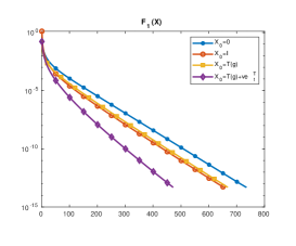
Refer to caption Refer to caption
Figure 1: Two-node Jackson network for Problem 777 of Table 1: Residual error per step in the three functional iterations F1,F2,F3subscript𝐹1subscript𝐹2subscript𝐹3F_{1},F_{2},F_{3} for different values of the initial matrix X0subscript𝑋0X_{0}. In the fourth graph, comparisons of the errors for the three iterations with X0=T(g)+ve1Tsubscript𝑋0𝑇𝑔𝑣superscriptsubscript𝑒1𝑇X_{0}=T(g)+ve_{1}^{T}.
00 I𝐼I T(g)𝑇𝑔T(g) T(g)+ve1T𝑇𝑔𝑣superscriptsubscript𝑒1𝑇T(g)+ve_{1}^{T}
F1subscript𝐹1F_{1} 58.6 54.7 65.7 69.1
F2subscript𝐹2F_{2} 37.2 34.8 40.0 28.9
F3subscript𝐹3F_{3} 59.5 56.2 73.3 52.2
00 I𝐼I T(g)𝑇𝑔T(g) T(g)+ve1T𝑇𝑔𝑣superscriptsubscript𝑒1𝑇T(g)+ve_{1}^{T}
F1subscript𝐹1F_{1} 735 654 668 472
F2subscript𝐹2F_{2} 466 416 421 297
F3subscript𝐹3F_{3} 242 215 217 152
Table 3: Two-node Jackson network for Problem 777 of Table 1: CPU time in seconds (left) and number of steps (right) required by the three fixed point iteration to arrive at a residual error at most 5.010145.0superscript10145.0\cdot 10^{-14} starting with different values of X0subscript𝑋0X_{0}.

We may observe that in this case CR is the most efficient algorithm and that the results of Theorems 4.3 and 4.5 are respected. In fact the iteration given by F3subscript𝐹3F_{3} with X0=T(g)+ve1Tsubscript𝑋0𝑇𝑔𝑣superscriptsubscript𝑒1𝑇X_{0}=T(g)+ve_{1}^{T} is the fastest one in terms of number of steps. While concerning the CPU time, the iteration F2subscript𝐹2F_{2} with X0=T(g)+ve1Tsubscript𝑋0𝑇𝑔𝑣superscriptsubscript𝑒1𝑇X_{0}=T(g)+ve_{1}^{T} is the fastest.

Table 4 concerns the case of a Two-node Jackson network with the choice of parameters given by λ1=5subscript𝜆15\lambda_{1}=5, λ2=0.7subscript𝜆20.7\lambda_{2}=0.7, μ1=2subscript𝜇12\mu_{1}=2, μ2=2subscript𝜇22\mu_{2}=2, p=0.5𝑝0.5p=0.5 and q=0.5𝑞0.5q=0.5. In this model, seen as a random walk in the quarter plane, the overall probability to move right is higher than the overall probability to move left, while the probability to move down is higher than the probability to move up. The table reports the CPU time in seconds (left) together with the number of steps required by the three iterations (right) to arrive at a residual error at most 5.010145.0superscript10145.0\cdot 10^{-14}. The computation of the symbol g(z)𝑔𝑧g(z) remains almost inexpensive even though the numerical length of the coefficient vector of the symbol g(z)𝑔𝑧g(z) is quite large, in fact the coefficients gisubscript𝑔𝑖g_{i} are computed in less than 0.0070.0070.007 seconds, and the size of the coefficient vector is 313131 for the coefficients of the negative powers of z𝑧z and 842484248424 for the coefficients of the positive powers, respectively. The numerical size of the correction is 28×693728693728\times 6937.

00 I𝐼I T(g)𝑇𝑔T(g) T(g)+ve1T𝑇𝑔𝑣superscriptsubscript𝑒1𝑇T(g)+ve_{1}^{T}
F1subscript𝐹1F_{1} 102.8 96.0 17.5 16.0
F2subscript𝐹2F_{2} 49.0 46.6 9.8 9.8
F3subscript𝐹3F_{3} 4981.0 4502.0 997.0 913.0
00 I𝐼I T(g)𝑇𝑔T(g) T(g)+ve1T𝑇𝑔𝑣superscriptsubscript𝑒1𝑇T(g)+ve_{1}^{T}
F1subscript𝐹1F_{1} 806 738 103 100
F2subscript𝐹2F_{2} 310 285 47 46
F3subscript𝐹3F_{3} 169 149 37 35
Table 4: Two-node Jackson network for λ1=5subscript𝜆15\lambda_{1}=5, λ2=0.7subscript𝜆20.7\lambda_{2}=0.7, μ1=2subscript𝜇12\mu_{1}=2, μ2=2subscript𝜇22\mu_{2}=2, p=0.5𝑝0.5p=0.5, q=0.5𝑞0.5q=0.5: CPU time in seconds (left) and number of steps (right) required by the three fixed point iteration to arrive at a residual error at most 5.010145.0superscript10145.0\cdot 10^{-14} starting with different values of X0subscript𝑋0X_{0}. Cyclic reduction requires 8 steps for the overall CPU time of 70.8 seconds.

For this problem, cyclic reduction provides the solution in 8 steps and in 70.870.870.8 seconds, while Newton iteration requires 8 steps and takes 782 seconds. In this case, due to the large size of the matrices involved in the computation of matrix inverses, CR takes a much larger time than the simple functional iterations given by F1subscript𝐹1F_{1} and F2subscript𝐹2F_{2} which either do not involve inversion or require just only one matrix inversion. While iteration given by F2subscript𝐹2F_{2} takes less than 10 seconds, the iteration given by F3subscript𝐹3F_{3}, even though is the fastest in terms of number of steps, needs a large CPU time. In fact, similarly to CR, it requires a matrix inversion at each step which becomes more expensive as the approximation approaches the limit. Newton iteration has the same convergence features as CR, however, the larger cost of solving a Sylvester equation makes this iteration much slower than the other ones at least for this problem.

In this model, increasing the values of λ1subscript𝜆1\lambda_{1} makes the size of the output much larger. In particular, with values λ16subscript𝜆16\lambda_{1}\geq 6, cyclic reduction breaks down for memory overflow while F2(X)subscript𝐹2𝑋F_{2}(X) provides the solution with a slight increase of the CPU time.

Figure 2 provides the solution G𝐺G in log scale where the Toeplitz part and the correction parts are separately represented.
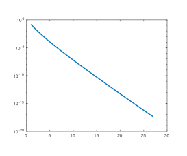
Refer to caption Refer to caption
Figure 2: Two-node Jackson network for λ1=5subscript𝜆15\lambda_{1}=5, λ2=0.7subscript𝜆20.7\lambda_{2}=0.7, μ1=2subscript𝜇12\mu_{1}=2, μ2=2subscript𝜇22\mu_{2}=2, p=0.5𝑝0.5p=0.5, q=0.5𝑞0.5q=0.5: Solution G𝐺G. In the upper part, the log-scale graph of the coefficients gisubscript𝑔𝑖g_{i} of the symbol for i0𝑖0i\leq 0 (left) and for i0𝑖0i\geq 0 (right). In the lower part the log-scale graph of the absolute value of the whole correction (left) together with a zoom (right).

7.2 Assistance from idle server

Here we consider a class of queueing models for a system with two servers and two queues. Arrivals to queues 1 and 2 occur as independent Poisson processes with parameters λ1subscript𝜆1\lambda_{1} and λ2subscript𝜆2\lambda_{2}, respectively. The service times of servers 1 and 2 are exponentially distributed with parameters μ1subscript𝜇1\mu_{1} and μ2subscript𝜇2\mu_{2} respectively. Each server serves its own queue according to a first-come-first-served discipline. If one of the queues is empty, the server for that queue assists the other server, doubling the latter’s service rate. If there is an arrival to a queue while its server is assisting the other queue, the server immediately ceases assisting and serves its own queue. This stochastic process is ergodic if and only if ρ1+ρ2<2subscript𝜌1subscript𝜌22\rho_{1}+\rho_{2}<2, where ρi=λi/μisubscript𝜌𝑖subscript𝜆𝑖subscript𝜇𝑖\rho_{i}=\lambda_{i}/\mu_{i}, i=1,2𝑖12i=1,2.

For this model, the matrices A1,A0,A1subscript𝐴1subscript𝐴0subscript𝐴1A_{-1},A_{0},A_{1} are given by A1=diag(2μ1,μ1,μ1,)subscript𝐴1diag2subscript𝜇1subscript𝜇1subscript𝜇1A_{-1}=\hbox{diag}(2\mu_{1},\mu_{1},\mu_{1},\ldots), A0=trid(μ2,λ1λ2μ1μ2,λ2)+(μ2μ1)e1e1Tsubscript𝐴0tridsubscript𝜇2subscript𝜆1subscript𝜆2subscript𝜇1subscript𝜇2subscript𝜆2subscript𝜇2subscript𝜇1subscript𝑒1superscriptsubscript𝑒1𝑇A_{0}=\hbox{trid}(\mu_{2},-\lambda_{1}-\lambda_{2}-\mu_{1}-\mu_{2},\lambda_{2})+(\mu_{2}-\mu_{1})e_{1}e_{1}^{T}, A1=λ1Isubscript𝐴1subscript𝜆1𝐼A_{1}=\lambda_{1}I.

In this example, we have chosen the values of the parameters in order that the numerical size of the matrix G𝐺G is substantially large, namely, λ1=0.01subscript𝜆10.01\lambda_{1}=0.01, λ2=2.9subscript𝜆22.9\lambda_{2}=2.9, μ1=0.03subscript𝜇10.03\mu_{1}=0.03, μ2=2.0subscript𝜇22.0\mu_{2}=2.0.

The situation is analogous to that of the second example in Section 7.1 where the methods based on functional iterations perform better than cyclic reduction and Newton iteration. The graphs in Figure 3 and the values in Table 5 synthesize the behavior of the algorithms. Cyclic reduction takes about 17 seconds of CPU while Newton iteration about 600 seconds. Slightly increasing the value of λ1subscript𝜆1\lambda_{1}, CR breaks down for memory overflow while functional iterations still compute correctly the solution G𝐺G.

Refer to caption Refer to caption
Figure 3: Assistance from idle server model from [24] for λ1=0.01subscript𝜆10.01\lambda_{1}=0.01, λ2=2.9subscript𝜆22.9\lambda_{2}=2.9, μ1=0.03subscript𝜇10.03\mu_{1}=0.03, μ2=2.0subscript𝜇22.0\mu_{2}=2.0: Residual error per step in the three functional iterations F1,F2,F3𝐹1subscript𝐹2subscript𝐹3F1,F_{2},F_{3} for different values of the initial matrix X0subscript𝑋0X_{0}. In the fourth graph, comparisons of the errors for the three iterations with X0=T(g)+ve1Tsubscript𝑋0𝑇𝑔𝑣superscriptsubscript𝑒1𝑇X_{0}=T(g)+ve_{1}^{T}.
00 I𝐼I T(g)𝑇𝑔T(g) T(g)+ve1T𝑇𝑔𝑣superscriptsubscript𝑒1𝑇T(g)+ve_{1}^{T}
F1subscript𝐹1F_{1} * * 204.8 191.6
F2subscript𝐹2F_{2} 16.4 13.7 4.6 3.9
F3subscript𝐹3F_{3} 405.1 402.6 218.3 183.6
00 I𝐼I T(g)𝑇𝑔T(g) T(g)+ve1T𝑇𝑔𝑣superscriptsubscript𝑒1𝑇T(g)+ve_{1}^{T}
F1subscript𝐹1F_{1} * * 844 782
F2subscript𝐹2F_{2} 42 40 10 9
F3subscript𝐹3F_{3} 26 25 9 7
Table 5: Assistance from idle server model from [24] for λ1=0.01subscript𝜆10.01\lambda_{1}=0.01, λ2=2.9subscript𝜆22.9\lambda_{2}=2.9, μ1=0.03subscript𝜇10.03\mu_{1}=0.03, μ2=2.0subscript𝜇22.0\mu_{2}=2.0: CPU time in seconds (left) and number of steps (right) required by the three fixed point iterations to arrive at a residual error at most 5.010145.0superscript10145.0\cdot 10^{-14} starting with different values of X0subscript𝑋0X_{0}. A “*” denotes a number of steps greater than 1000. Cyclic reduction requires 5 steps and 17 seconds of CPU time.

7.3 Random walk in the quarter plane

Here we consider an example where the condition A1𝟏>A1𝟏subscript𝐴11subscript𝐴11A_{-1}{\bm{1}}>A_{1}{\bm{1}} is satisfied everywhere exept in the first component. The example describes a random walk in the quarter plane where a particle can occupy positions in a grid and we know the probabilities that the particle moves to the neighboring positions. In order to better describe the test problem, we denote H=(hi,j)i,j=1,1𝐻subscriptsubscript𝑖𝑗formulae-sequence𝑖𝑗11H=(h_{i,j})_{i,j=-1,1} the matrix with the probabilities of transition in the inner part of the quarter plane, while we denote Y=(yi,j)𝑌subscript𝑦𝑖𝑗Y=(y_{i,j}) the 3×2323\times 2 matrix with the probabilities of transition in the y𝑦y axis. These two matrices fully describe the coefficients Aisubscript𝐴𝑖A_{i} which can be written as Ai=T(ai)+Eisubscript𝐴𝑖𝑇subscript𝑎𝑖subscript𝐸𝑖A_{i}=T(a_{i})+E_{i} where ai(z)=j=11hi,jzjsubscript𝑎𝑖𝑧superscriptsubscript𝑗11subscript𝑖𝑗superscript𝑧𝑗a_{i}(z)=\sum_{j=-1}^{1}h_{i,j}z^{j} and Ei=e1[yi,0hi,0,yi,1hi,1,0,]subscript𝐸𝑖subscript𝑒1subscript𝑦𝑖0subscript𝑖0subscript𝑦𝑖1subscript𝑖10E_{i}=e_{1}[y_{i,0}-h_{i,0},y_{i,1}-h_{i,1},0,\ldots], compare with (4).

The random walk of this example is obtained with the values

H=19[101200221],Y=13[110100]formulae-sequence𝐻19matrix101200221𝑌13matrix110100H=\frac{1}{9}\begin{bmatrix}1&0&1\\ 2&0&0\\ 2&2&1\end{bmatrix},\quad Y=\frac{1}{3}\begin{bmatrix}1&1\\ 0&1\\ 0&0\end{bmatrix}

so that the condition A1𝟏>A1𝟏subscript𝐴11subscript𝐴11A_{-1}{\bm{1}}>A_{1}{\bm{1}} is satisfied in all the components but the first.

For this problem, there exist two nonnegative solutions G𝐺G and G^^𝐺\widehat{G} to equation (1) which satisfy the inequality GG^𝐺^𝐺G\leq\widehat{G}. Moreover G^^𝐺\widehat{G} is stochastic while G𝐺G is substochastic. The two solutions have the same symbol g(z)𝑔𝑧g(z) and differ only for the correction part. Starting with X0=0subscript𝑋00X_{0}=0 or with X0=T(g)subscript𝑋0𝑇𝑔X_{0}=T(g) the sequences generated by the functional iterations converge to G𝐺G. Starting with X0=Isubscript𝑋0𝐼X_{0}=I or X0=T(g)+ve1Tsubscript𝑋0𝑇𝑔𝑣superscriptsubscript𝑒1𝑇X_{0}=T(g)+ve_{1}^{T} the sequences converge to G^^𝐺\widehat{G}, while CR and Newton iteration converge to G𝐺G.

The results of this test are summarized in Table 6. Both CR and Newton iteration take 23 steps in order to arrive at numerical convergence. However CR takes more than 8 minutes of CPU time while Newton iteration just 3.4 seconds. The large amount of CPU time taken by CR is due to the fact that the inverse matrices involved at each step of CR are QT matrices with a correction having a size which increases step after step and reaches values larger than 106superscript10610^{6}, while Newton iteration involves QT matrices with corrections having almost the same size of the correction of G𝐺G which is 126×3612636126\times 36. The growth of the sizes of the correction matrices in the algorithms is an issue which deserves further analysis.

Functional iterations F1,F2subscript𝐹1subscript𝐹2F_{1},F_{2} and F3subscript𝐹3F_{3} with X0=0subscript𝑋00X_{0}=0 or with X0=T(g)subscript𝑋0𝑇𝑔X_{0}=T(g) take a large number of steps to converge numerically to G𝐺G while with X0=Isubscript𝑋0𝐼X_{0}=I or X0=T(g)+ve1Tsubscript𝑋0𝑇𝑔𝑣superscriptsubscript𝑒1𝑇X_{0}=T(g)+ve_{1}^{T} the number of iterations is much smaller but the limit of the sequences is the stochastic solution G^^𝐺\widehat{G} which is not the minimal one.

For this problem, the combination of few steps of CR followed by few steps of Newton iteration provide a substantial acceleration in terms of CPU time. In fact, the first iterations of CR, involving matrices of small size, have a low cost. The last few steps of CR, which have a much higher cost, are replaced by Newton steps.

F1subscript𝐹1F_{1} F2subscript𝐹2F_{2} F3subscript𝐹3F_{3} F1subscript𝐹1F_{1} F2subscript𝐹2F_{2} F3subscript𝐹3F_{3} CR Newton CR+Newton
iter * * * 285 205 119 23 23 15+10
CPU * * * 3.1 2.3 2.6 524 3.4 0.4+1.5
Table 6: Random walk in the quarter plane: Number of iterations and CPU time in seconds. From left to right: fixed point iterations with X0=T(g)subscript𝑋0𝑇𝑔X_{0}=T(g), fixed point iterations with X0=T(g)+ve1Tsubscript𝑋0𝑇𝑔𝑣superscriptsubscript𝑒1𝑇X_{0}=T(g)+ve_{1}^{T}, cyclic reduction, Newton iteration with X0=0subscript𝑋00X_{0}=0, combination of cyclic reduction and Newton iteration. A “*” denotes more than 10000 iterations and a CPU larger than 1000 seconds. Starting the iterations with X0=T(g)+ve1Tsubscript𝑋0𝑇𝑔𝑣superscriptsubscript𝑒1𝑇X_{0}=T(g)+ve_{1}^{T} generates sequences converging to the stochastic solution G^^𝐺\widehat{G}, while starting with X0=0subscript𝑋00X_{0}=0 or applying CR, Newton iteration and their combinations generate sequences converging to the minimal (substochastic) solution G𝐺G.

8 Conclusions

We have analyzed quadratic matrix equations encountered in the solution of random walk in the quarter plane where the solution of interest is the minimal nonnegative solution G𝐺G. This class of equations is characterized by matrix coefficients with infinite size which belong to the class 𝒬𝒯𝒬𝒯\mathcal{QT} of Quasi-Toeplitz matrices. We have provided a perturbation analysis of G𝐺G, introduced some fixed point algorithms for computing G𝐺G and compared their convergence speed. The algorithms rely on the properties of 𝒬𝒯𝒬𝒯\mathcal{QT} matrices recently investigated in [6]. Numerical experiments show that in many cases the CPU time and the memory resources required by our approach are significantly inferior to the ones required by the algorithm of cyclic reduction, which is considered as the algorithm of choice for this class of problems. The effectiveness of Newton iteration depends on the growth of the sizes of the correction part in the QT matrices generated by the algorithm.

References

  • [1] R. Bartels and G. Stewart. Solution of the matrix equation AX+XB=C𝐴𝑋𝑋𝐵𝐶AX+XB=C: Algorithm 432. Comm. ACM, 15:820–826, 1972.
  • [2] D. A. Bini, G. Latouche, and B. Meini. Numerical methods for structured Markov chains. Numerical Mathematics and Scientific Computation. Oxford University Press, New York, 2005. Oxford Science Publications.
  • [3] D. A. Bini, S. Massei, and B. Meini. Semi-infinite quasi-Toeplitz matrices with applications to QBD stochastic processes. Math. Comp., 87(314):2811–2830, 2018.
  • [4] D. A. Bini, S. Massei, B. Meini, and L. Robol. On quadratic matrix equations with infinite size coefficients encountered in QBD stochastic processes. Numer. Linear Algebra Appl., 25(6):2128, 12, 2018.
  • [5] D. A. Bini, S. Massei, B. Meini, and L. Robol. Matrix analytic methods for reflected random walks with restart. In preparation, 2019.
  • [6] D. A. Bini, S. Massei, and L. Robol. Quasi-Toeplitz matrix arithmetic: a MATLAB toolbox. Numerical Algorithms, 81(2):741–769, 2019.
  • [7] D. A. Bini and B. Meini. On the solution of a nonlinear matrix equation arising in queueing problems. SIAM J. Matrix Anal. Appl., 17(4):906–926, 1996.
  • [8] D. A. Bini and B. Meini. Improved cyclic reduction for solving queueing problems. Numer. Algorithms, 15(1):57–74, 1997.
  • [9] G. Fayolle, R. Iasnogorodski, and V. Malyshev. Random walks in the quarter plane, volume 40 of Probability Theory and Stochastic Modelling. Springer, Cham, second edition, 2017. Algebraic methods, boundary value problems, applications to queueing systems and analytic combinatorics.
  • [10] L. Flatto and S. Hahn. Two parallel queues created by arrivals with two demands I. SIAM Journal on Applied Mathematics, 44(5):1041–1053, 1984.
  • [11] L. Haque, Y. Q. Zhao, and L. Liu. Sufficient conditions for a geometric tail in a QBD process with many countable levels and phases. Stochastic Models, 21(1):77–99, 2005.
  • [12] P. Henrici. Applied and computational complex analysis. Vol. 1. Wiley Classics Library. John Wiley & Sons, Inc., New York, 1988. Power series—integration—conformal mapping—location of zeros, Reprint of the 1974 original, A Wiley-Interscience Publication.
  • [13] N. J. Higham and H.-M. Kim. Numerical analysis of a quadratic matrix equation. IMA J. Numer. Anal., 20(4):499–519, 2000.
  • [14] M. Kobayashi and M. Miyazawa. Revisiting the tail asymptotics of the double QBD process: refinement and complete solutions for the coordinate and diagonal directions. In Matrix-analytic methods in stochastic models, volume 27 of Springer Proc. Math. Stat., pages 145–185. Springer, New York, 2013.
  • [15] D. P. Kroese, W. R. W. Scheinhardt, and P. G. Taylor. Spectral properties of the tandem Jackson network, seen as a quasi-birth-and-death process. Ann. Appl. Probab., 14(4):2057–2089, 2004.
  • [16] G. Latouche. Newton’s iteration for non-linear equations in Markov chains. IMA J. Numer. Anal., 14(4):583–598, 1994.
  • [17] G. Latouche, S. Mahmoodi, and P. Taylor. Level-phase independent stationary distributions for GI/M/1-type Markov chains with infinitely-many phases. Performance Evaluation, 70(9):551–563, 2013.
  • [18] G. Latouche, G. T. Nguyen, and P. G. Taylor. Queues with boundary assistance: the effects of truncation. Queueing Syst., 69(2):175–197, 2011.
  • [19] G. Latouche and V. Ramaswami. Introduction to matrix analytic methods in stochastic modeling. ASA-SIAM Series on Statistics and Applied Probability. Society for Industrial and Applied Mathematics (SIAM), Philadelphia, PA; American Statistical Association, Alexandria, VA, 1999.
  • [20] G. Latouche and P. Taylor. Truncation and augmentation of level-independent QBD processes. Stochastic Process. Appl., 99(1):53–80, 2002.
  • [21] B. Meini. New convergence results on functional iteration techniques for the numerical solution of M/G/1𝑀𝐺1M/G/1 type Markov chains. Numer. Math., 78(1):39–58, 1997.
  • [22] M. Miyazawa. Light tail asymptotics in multidimensional reflecting processes for queueing networks. TOP, 19(2):233–299, 2011.
  • [23] M. Miyazawa and Y. Q. Zhao. The stationary tail asymptotics in the GI/G/1𝐺𝐼𝐺1GI/G/1-type queue with countably many background states. Adv. in Appl. Probab., 36(4):1231–1251, 2004.
  • [24] A. J. Motyer and P. G. Taylor. Decay rates for quasi-birth-and-death processes with countably many phases and tridiagonal block generators. Adv. Appl. Prob., 38:522–544, 2006.
  • [25] M. F. Neuts. Matrix-geometric solutions in stochastic models: An algorithmic approach, volume 2 of Johns Hopkins Series in the Mathematical Sciences. Johns Hopkins University Press, Baltimore, Md., 1981.
  • [26] T. Ozawa. Stability condition of a two-dimensional qbd process and its application to estimation of efficiency for two-queue models. Performance Evaluation, 130:101 – 118, 2019.
  • [27] T. Ozawa and M. Kobayashi. Exact asymptotic formulae of the stationary distribution of a discrete-time two-dimensional QBD process. Queueing Systems, 90(3):351–403, Dec 2018.
  • [28] L. Robol. Rational Krylov and ADI iteration for infinite size quasi-Toeplitz matrix equations. arXiv:1907.02753, pages 1–24, 2019.
  • [29] Y. Sakuma and M. Miyazawa. On the effect of finite buffer truncation in a two-node Jackson network. J. Appl. Probab., 42(1):199–222, 2005.
  • [30] D. Stanford, W. Horn, and G. Latouche. Tri-layered QBD processes with boundary assistance for service resources. Stochastic Models, 22(3):361–382, 2006.
  • [31] Y. Takahashi, K. Fujimoto, and N. Makimoto. Geometric decay of the steady-state probabilities in a quasi-birth-and-death process with a countable number of phases. Communications in Statistics. Part C: Stochastic Models, 17(1):1–24, 2001.