Homogenized Flux-Body Force Treatment of Compressible Viscous Porous Wall Boundary Conditions

Abstract

A homogenization approach is proposed for the treatment of porous wall boundary conditions in the computation of compressible viscous flows. Like any other homogenization approach, it eliminates the need for pore-resolved fluid meshes and therefore enables practical flow simulations in computational fluid domains with porous wall boundaries. Unlike alternative approaches however, it does not require prescribing a mass flow rate and does not introduce in the computational model a heuristic discharge coefficient. Instead, it models the inviscid flux through a porous wall surrounded by the flow as a weighted average of the inviscid flux at an impermeable surface and that through pores. It also introduces a body force term in the governing equations to account for friction loss along the pore boundaries. The source term depends on the thickness of the porous wall and the concept of an equivalent single pore. The feasibility of the latter concept is demonstrated using low-speed permeability test data for the fabric of the Mars Science Laboratory parachute canopy. The overall homogenization approach is illustrated with a series of supersonic flow computations through the same fabric and verified using supersonic, pore-resolved numerical simulations.

1 Introduction

Porous walls and membranes appear in a wide range of scientific and engineering applications. These include, to name only a few, filtration processes [27, 11, 21] to separate particulates or molecules from a bulk fluid, the cooling of gas turbines via multiperforated plates [1, 24, 23, 25], light weight canopies for low density supersonic decelerators [18, 17, 9, 15, 14], and windbreaks or shelterbelts [16, 29, 37] to reduce the relative flow speed and maintain stability. For most of these large-scale engineering applications, pore-resolved CFD computations remain unpractical, if not unaffordable. Therefore, the high-precision and yet computationally efficient treatment of porous wall boundary conditions in CFD computations is crucial for enabling flow simulations that further the understanding of the effects of porous materials and can assist in the development of membrane-related processes and technologies.

The modeling of fluid flow through a porous wall or membrane has been inspired by a variety of investigations of flows in porous media. In [18, 36, 34, 9, 35], a modified Darcy’s law was coupled with Ergun’s equation to construct an internal pressure jump condition for the incompressible or low-Mach Navier-Stokes equations and account for the material porosity of a canopy in the simulation of parachute fluid-structure interactions. In [40] and [37], the flow associated with a windbreak similar to a plant canopy was modeled by adding a local, momentum extraction, source term near the windbreak. The pressure-loss coefficient in the source term was calibrated using the pressure drop across the windbreak, as well as the flow momentum measured in related wind tunnel experiments [16]. In [27] and [11], the analysis of the cross-flow filtration was performed by numerically simulating the transport of solutes or particles in a tube with porous walls using the Navier-Stokes equations and applying the slip wall boundary condition, as advocated in [3]. Notably, all of the aforementioned modeling approaches are limited to the incompressible flow regime.

Only a few approaches for modeling the effects of permeability on high Mach number compressible flows have been documented so far. Those approaches have combined Darcy’s law with the continuity equation [26], or derived compressible variants of Darcy’s law from the continuity equation and the force balance equation between drag and the pressure drop across an element of a porous material [32, 31]. For flow computations associated with film-cooling in gas turbines operating at high-speed, the following works are noteworthy. In [1], the treatment of the porous wall boundary condition was performed using a mass inflow condition with white noise in the mass flow rate. In [23], a homogeneous model was proposed for a multiperforated plate where the homogenized mass flux is related to a constant discharge coefficient estimated from pore-resolved numerical simulations.

Here, an alternative homogenization approach is proposed for the treatment of porous wall boundary conditions in the numerical simulation of compressible viscous flows through permeable surfaces. Unlike the aforementioned approaches, it does not require prescribing a mass flow rate nor introduces an empirical discharge coefficient in the computational model. Instead, it models the inviscid flux through a porous wall as a weighted average of the inviscid flux at an impermeable surface and that through pores. To account for the loss of friction along the pore boundaries, it introduces a body force term in the governing equations that depends on the thickness of the porous wall and the concept of an “equivalent pore” – that is, a single pore whose geometry and dimensions are such that when inserted at the center of a unit cell, the void fraction of the cell matches that of the fabric of interest. The feasibility of such a concept is demonstrated using low-speed permeability experimental data for the fabric of the Mars Science Laboratory parachute canopy. The overall homogenization approach can be implemented in any finite difference, finite volume, or finite element semi-discretization scheme. It is illustrated with a series of supersonic porous flow problems with Martian atmosphere free-stream conditions and verified using pore-resolved numerical simulations.

The remainder of the paper is organized as follows. First, the governing equations are specified in Section 2. Next, the proposed homogenization approach is presented in Section 3 and its verification is performed in Section 4. Finally, conclusions are offered in Section 5.

2 Governing equations

Throughout this paper, flows are assumed to be compressible as well as viscous and are governed by the Navier-Stokes equations. These can be written in conservation form as follows

$$\dfrac{\partial\bm{W}}{\partial t}+\nabla\cdot\mathcal{F}(\bm{W})=\nabla\cdot\mathcal{G}(\bm{W})\,,$$ (1)

where $\bm{W}$ denotes the vector of the conservative variables describing the fluid state, $t$ denotes time, and $\mathcal{F}(\bm{W})$ and $\mathcal{G}(\bm{W})$ are the inviscid and viscous flux tensor functions of the conservative variables, respectively. Specifically,

$$\bm{W}=\begin{pmatrix}\rho\\[11.38109pt] \rho\bm{v}\\[11.38109pt] E\end{pmatrix},\quad\mathcal{F}(\bm{W})=\begin{pmatrix}\rho\bm{v}\\[5.69054pt] \rho\bm{v}\otimes\bm{v}+p\mathcal{I}\\[7.11317pt] \bigl{(}E+p\bigr{)}\bm{v}\end{pmatrix},\quad\mathrm{and}\quad\mathcal{G}(\bm{W})=\begin{pmatrix}0\\[7.11317pt] {\uptau}\\[4.2679pt] {\uptau}\bm{\cdot}\bm{v}-\bm{q}\end{pmatrix},$$ (2)

where $\rho$, $\bm{v}$, and $E$ denote the density, velocity, and total energy per unit volume of the fluid, respectively, and $\otimes$ denotes the Hadamard product. The fluid velocity and total energy per unit volume can be written as

$$\bm{v}=(u,v,w)^{T}\quad\textrm{and}\quad E=\rho e+\dfrac{1}{2}\rho(u^{2}+v^{2}+w^{2})\,,$$ (3)

where the superscript $T$ designates the transpose and $e$ denotes the specific (i.e., per unit of mass) internal energy. In the physical inviscid flux tensor $\mathcal{F}$, $p$ is the static pressure and $\mathcal{I}\in\mathbb{R}^{3}$ is the identity matrix. In the viscous flux tensor $\mathcal{G}$, ${\uptau}$ and $\bm{q}$ denote the viscous stress tensor and heat flux vector, respectively, and are defined as follows

$${\uptau}=\mu(\nabla^{T}\bm{v}+\nabla\bm{v})-\dfrac{2}{3}\mu(\nabla\bm{\cdot}\bm{v})\mathcal{I}\quad\mathrm{and}\quad\bm{q}=-\kappa\nabla T,$$ (4)

where $\mu$ is the dynamic shear viscosity of the fluid, $\kappa$ is its thermal conductivity, and $T$ is its temperature.

For simplicity, but without any loss of generality, the system of equations (1) is closed by assuming that the gas is ideal, calorically perfect, and therefore governed by

$$p=\rho RT\quad\mathrm{and}\quad e=\frac{R}{\gamma-1}T,$$ (5)

where $R$ and $\gamma$ are the gas constant and specific heat ratio, respectively.

3 Homogenized flux-body force approach

Consider as a backdrop for the homogenization approach described herein the three-dimensional, porous flow model problem graphically depicted in Fig. 1. The computational fluid domain is a three-dimensional, orthogonal box with a square cross section (the generalization to an arbitrarily-shaped computational fluid domain is straightforward). It contains at its center a porous wall of a finite thickness (shown in blue color) whose edges are flushed with four of the six surface boundaries of the computational fluid domain. The free-stream velocity of the flow is perpendicular to the surface of the wall and periodic boundary conditions are prescribed in both transverse directions.

Figure 1: Porous flow model problem: porous wall, computational fluid domain, and periodic boundary conditions.

Assuming that the porous wall is reasonably thin, it can be modeled as a surface denoted here by $\Omega$. This surface is discretized by a mesh whose typical element size is much larger than the pore size. Hence, given a scalar or vector quantity $\phi$ defined in $\Omega$, a homogenized semi-discrete counterpart $\bar{\phi}$, where homogenization is performed in both transverse directions and designated by an overline, is defined here as

$$\bar{\phi}=\displaystyle{\frac{\int_{\Omega}\phi\,d\Omega}{|\Omega|}}\,,$$ (6)

where $|\Omega|$ denotes the area of the surface $\Omega$.

Due to symmetry (see Fig. 1), both homogenized transverse velocity components $\bar{v}$ and $\bar{w}$ are zero. For this reason, the homogenized version of Eq. 1 inside the porous wall can be written as

$$\begin{split}\frac{\partial\bar{\rho}}{\partial t}+\frac{\partial\overline{\rho u}}{\partial x}&=0\,,\\ \frac{\partial\overline{\rho u}}{\partial t}+\frac{\partial\overline{\rho uu+p}}{\partial x}&=\frac{\partial\overline{\tau_{xx}}}{\partial x}+\underbrace{\left[{\frac{\overline{\partial\tau_{xy}}}{\partial y}}+{\frac{\overline{\partial\tau_{xz}}}{\partial z}}\right]}_{\textrm{to be modeled}},\\ \frac{\partial\overline{E}}{\partial t}+\frac{\partial\overline{(E+p)u}}{\partial x}&=\frac{\partial\overline{\tau_{xx}u-q_{x}}}{\partial x}+\underbrace{\left[{\frac{\overline{\partial\tau_{xy}u}}{\partial y}}+{\frac{\overline{\partial\tau_{xz}u}}{\partial z}}\right]}_{\textrm{to be modeled}},\end{split}$$ (7)

where

• $\tau_{xx}$, $\tau_{xy}$, and $\tau_{xz}$ are the components of the viscous stress tensor ${\uptau}$ given by

  $$\tau_{xx}=\mu\left(\frac{4}{3}\frac{\partial u}{\partial x}-\frac{2}{3}\frac{\partial v}{\partial y}-\frac{2}{3}\frac{\partial w}{\partial z}\right),\quad\tau_{xy}=\mu\left(\frac{\partial u}{\partial y}+\frac{\partial v}{\partial x}\right),\quad\tau_{xz}=\mu\left(\frac{\partial u}{\partial z}+\frac{\partial w}{\partial x}\right).$$ (8)

• $q_{x}$ is the $x$-component of the heat flux vector $\bm{q}$ whose expression is given by

  $$q_{x}=-\kappa\frac{\partial T}{\partial x}\,.$$ (9)

• The averaged terms $\overline{\partial\tau_{xy}/\partial y}+\overline{\partial\tau_{xz}/\partial z}$ and $\overline{\partial\tau_{xy}u/\partial y}+\overline{\partial\tau_{xz}u/\partial z}$ are shown between brackets to emphasize that: while they vanish in the cross sections away from the porous wall – due to the fact that they contain only partial derivatives with respect to the directions of homogenization $y$ and $z$ – they represent the averaged friction loads on the pore boundary and therefore require subgrid scale modeling; and hence they will be reintroduced in Section 3.3 in the form of a body force model.

From (8), (9), and the periodic nature of the prescribed boundary conditions (see Fig. 1), it follows that the expressions for the averaged, wall normal, viscous flux terms $\partial\overline{\tau_{xx}}/\partial x$ and $\partial\left(\overline{\tau_{xx}u-q_{x}}\right)/\partial x$ can be simplified as follows

$$\overline{\tau_{xx}}=\frac{4}{3}\mu\frac{\partial\overline{u}}{\partial x}\quad\textrm{ and }\quad\overline{\tau_{xx}u-q_{x}}=\frac{4}{3}\mu\overline{\frac{\partial u}{\partial x}u}+\kappa\frac{\partial\overline{T}}{\partial x}\,,$$ (10)

which transforms Eq. 7 into the following, more specific, homogenized governing equations inside the porous wall

$$\begin{split}\frac{\partial\bar{\rho}}{\partial t}+\frac{\partial\overline{\rho u}}{\partial x}&=0\,,\\ \frac{\partial\overline{\rho u}}{\partial t}+\frac{\partial\overline{\rho uu+p}}{\partial x}&=\frac{\partial}{\partial x}\left(\frac{4}{3}\mu\frac{\partial\overline{u}}{\partial x}\right)+\underbrace{\left[{\frac{\overline{\partial\tau_{xy}}}{\partial y}}+{\frac{\overline{\partial\tau_{xz}}}{\partial z}}\right]}_{\textrm{to be modeled}}\,,\\ \frac{\partial\overline{E}}{\partial t}+\frac{\partial\overline{(E+p)u}}{\partial x}&=\frac{\partial}{\partial x}\left(\frac{4}{3}\mu\overline{\frac{\partial u}{\partial x}u}+\kappa\frac{\partial\overline{T}}{\partial x}\right)+\underbrace{\left[{\frac{\overline{\partial\tau_{xy}u}}{\partial y}}+{\frac{\overline{\partial\tau_{xz}u}}{\partial z}}\right]}_{\textrm{to be modeled}}.\end{split}$$ (11)

For the sake of clarity, the homogenization approach proposed herein is described in the next two subsections not only in the backdrop of the model porous flow problem illustrated in Fig. 1 but also in the context of a cell-centered Finite Volume (FV) approximation method, where the gradients underlying the viscous fluxes are semi-discretized by a finite difference scheme and for simplicity, but without any loss of generality, the CFD mesh is assumed to be structured and body-fitted. In this case, each computational cell ${\mathcal{C}}_{i}$ is a primal element of the CFD mesh, $i$ is the center point of ${\mathcal{C}}_{i}$ where the semi-discrete fluid state vector is defined, and the boundary surface (cell facet) $\partial{\mathcal{C}}_{ij}$ shared by two cells $\mathcal{C}_{i}$ and $\mathcal{C}_{j}$, where $j$ is such that the line $(i,j)$ traverses the porous wall, lies along the surface of this wall (see Fig. 2). However, as will be noted wherever appropriate within the next two subsections, the generalizations of this approach to a vertex-based FV approximation method where the viscous fluxes are semi-discretized by a Finite Element (FE) method and to unstructured meshes as well as an arbitrary orientation of the porous wall with respect to the global reference frame, are straightforward. Furthermore, the homogenization approach described below is not limited to body-fitted CFD methods: it is equally applicable to embedded/immersed boundary methods. In particular, it is well-suited for the FInite Volume method with Exact two-material Riemann problems (FIVER) [38, 19, 22, 12, 4] (see also Appendix A). As a matter of fact, all numerical results with the porosity model reported in Section 4 are obtained using non body-fitted CFD meshes and the Embedded Boundary Method (EBM) FIVER. In short, the proposed homogenization approach for the treatment of porous wall boundary conditions can be incorporated in any semi-discretization or discretization method.

Figure 2: Schematic of the homogenized inviscid flux: context of a cell-centered finite volume approximation method on a body-fitted CFD mesh (central $x$-$y$ plane view).

3.1 Homogenized inviscid flux

Let $\alpha$ denote the void fraction or porosity of the porous wall. It can be expressed as

$$\alpha=\displaystyle{\frac{|\Omega|^{\textrm{pore}}}{|\Omega|}}$$ (12)

where $|\Omega^{\textrm{pore}}|$ denotes the total area occupied by the pores in the surface $\Omega$.

Consider first the two following extreme cases:

• $\alpha=1$, which corresponds to the no-wall configuration. In this case, the inviscid fluxes through the (nonexistent) porous wall can be approximated as usual, for example, by an approximate Riemann solver such as Roe’s solver [30]. This can be written as (see Fig. 2)

  $$\bm{F}_{ij}=-\bm{F}_{ji}=|{\partial\mathcal{C}}_{ij}|\,\bm{F}^{\textrm{{Roe}}}(\bm{W}_{i},\bm{W}_{j},n_{ij})\,,$$ (13)

  where $\bm{F}_{ij}$ is the numerical inviscid flux function associated with the inviscid flux vector in the $x$-direction, $\bm{F}$, $n_{ij}$ is the unit outward normal to $\partial{\mathcal{C}}_{ij}$ – in this case, $n_{ij}$ is parallel to the $x$-direction – and $|\partial{\mathcal{C}}_{ij}|$ denotes the area of $\partial{\mathcal{C}}_{ij}$.

• $\alpha=0$, which corresponds to the impermeable wall configuration. In this case, the inviscid fluxes can also be approximated as usual – that is, as wall boundary fluxes as follows (see Fig. 2)

  $$\bm{F}_{ij}=|\partial{\mathcal{C}}_{ij}|\,\bm{F}^{\textrm{{imp-wall}}}(\bm{W}_{i},n_{ij})\quad\textrm{ and }\quad\bm{F}_{ji}=|\partial{\mathcal{C}}_{ji}|\,\bm{F}^{\textrm{{imp-wall}}}(\bm{W}_{j},n_{ji})\,,$$ (14)

where $|\partial{\mathcal{C}}_{ji}|=|\partial{\mathcal{C}}_{ij}|$, $n_{ji}=-n_{ij}$, and $\bm{F}^{\textrm{{imp-wall}}}(\bm{W}_{i},n_{ij})$ and $\bm{F}^{\textrm{{imp-wall}}}(\bm{W}_{j},n_{ji})$ are computed using the physical inviscid flux tensor $\mathcal{F}$, $n_{ij}$, and the standard, impermeable wall boundary conditions.

Hence, the main idea here is to compute, for any nontrivial porosity value $0<\alpha<1$, the homogenized, numerical inviscid flux functions through the porous wall $\bm{F}^{\textrm{ave}}_{ij}$ and $\bm{F}^{\textrm{ave}}_{ji}$ as convex combinations of (13) and (14) using however averaged values of the fluid state vectors – that is,

$$\begin{split}\bm{F}^{\textrm{ave}}_{ij}&=|\partial{\mathcal{C}}_{ij}|\left(\alpha\bm{F}^{\textrm{{Roe}}}(\overline{\bm{W}}_{i},\overline{\bm{W}}_{j},n_{ij})+(1-\alpha)\bm{F}^{\textrm{imp-wall}}(\overline{\bm{W}}_{i},n_{ij})\right)\,,\\ \bm{F}^{\textrm{ave}}_{ji}&=|\partial{\mathcal{C}}_{ji}|\left(\alpha\bm{F}^{\textrm{{Roe}}}(\overline{\bm{W}}_{j},\overline{\bm{W}}_{i},n_{ji})+(1-\alpha)\bm{F}^{\textrm{imp-wall}}(\overline{\bm{W}}_{j},n_{ji})\right)\,,\end{split}$$ (15)

where averaging is performed as in (6). The second-order extension of the above approximations using the classical Monotonic Upstream-centered Scheme for Conservation Laws (MUSCL) is straightforward.

The above computation (15) is illustrated in Fig. 2, where the computational cells adjacent to the porous wall are divided into two parts: one part attached to a hole (colored in blue) representing the pores, collectively; and another part attached to the wall (colored in red). Accordingly, the flux through the porous wall $\bm{F}^{\textrm{ave}}_{ij}$ consists of the flux through the hole (13) and that at the impermeable part of the wall (see Eq. 14).

Note that by construction, the proposed homogenization of the numerical inviscid flux function (15) associated with the inviscid flux vector in the $x$-direction $\bm{F}$ conserves mass and energy; it also guarantees that the impermeable part of the numerical flux has zero mass and energy components.

The generalization of the inviscid flux homogenization procedure described above to the case of a vertex-based FV method with control volumes (dual cells) ${\mathcal{C}}_{i}$ – in which case a wall boundary grid point $i$ and not a wall boundary cell facet $\partial{\mathcal{C}}_{ij}$ lies on the porous wall – is simply accomplished using the concept of half dual cells. The generalization of this procedure to an arbitrary direction of the outward normal to the wall $n_{ij}$ and to unstructured meshes is straightforward, because most if not all approximate Riemann solvers are essentially one-dimensional local solvers that propagate information in the direction normal to the considered facet of the control volume boundary.

3.2 Homogenized viscous flux

The spirit of the approach described in Section 3.1 for the numerical inviscid fluxes is followed here to model each numerical viscous flux in the wall normal direction (which in this case is the $x$-direction), $\bm{G}_{ij}^{\textrm{ave}}$ and $\bm{G}_{ji}^{\textrm{ave}}$, as a convex combination of the numerical viscous flux at an impermeable surface and that through pores computed using averaged fluid state vectors. Recalling that the terms shown between brackets in Eq. 11 vanish because they contain derivatives in the homogenized directions, choosing to approximate the gradients in the viscous fluxes by, for example, the second-order central finite differencing, and assuming that the dynamic shear viscosity $\mu$ and fluid thermal conductivity $\kappa$ are constant, the homogenization of the numerical viscous flux functions through the porous wall can be carried out as follows (see Fig. 2)

$$\begin{split}\bm{G}_{ij}^{\textrm{ave}}=|\partial{\mathcal{C}}_{ij}|\left(\alpha\underbrace{\begin{pmatrix}0\\ \frac{4}{3}\mu\frac{\overline{u}_{j}-\overline{u}_{i}}{\delta_{x}}\\ \frac{4}{3}\mu\left(\frac{\overline{u}_{j}-\overline{u}_{i}}{\delta_{x}}\right)\left(\frac{\overline{u}_{i}+\overline{u}_{j}}{2}\right)+\kappa\frac{\overline{T}_{j}-\overline{T}_{i}}{\delta_{x}}\end{pmatrix}}_{\bm{G}_{ij}^{\textrm{pore}}}\,+\,(1-\alpha)\underbrace{\begin{pmatrix}0\\ \frac{4}{3}\mu\frac{\overline{u}^{\,\textrm{be}}_{j}-\overline{u}_{i}}{\delta_{x}}\\ \frac{4}{3}\mu\left(\frac{\overline{u}^{\,\textrm{be}}_{j}-\overline{u}_{i}}{\delta_{x}}\right)\left(\frac{\overline{u}_{i}+\overline{u}^{\,\textrm{be}}_{j}}{2}\right)+\kappa\frac{\overline{T}^{\,\textrm{be}}_{j}-\overline{T}_{i}}{\delta_{x}}\end{pmatrix}}_{\bm{G}_{ij}^{\textrm{imp-wall}}}\right)\,,\\ \bm{G}_{ji}^{\textrm{ave}}=|{\partial\mathcal{C}}_{ij}|\left(\alpha\underbrace{\begin{pmatrix}0\\ \frac{4}{3}\mu\frac{\overline{u}_{i}-\overline{u}_{j}}{\delta_{x}}\\ \frac{4}{3}\mu\left(\frac{\overline{u}_{i}-\overline{u}_{j}}{\delta_{x}}\right)\left(\frac{\overline{u}_{i}+\overline{u}_{j}}{2}\right)+\kappa\frac{\overline{T}_{i}-\overline{T}_{j}}{\delta_{x}}\end{pmatrix}}_{\bm{G}_{ji}^{\textrm{pore}}}\,+\,(1-\alpha)\underbrace{\begin{pmatrix}0\\ \frac{4}{3}\mu\frac{\overline{u}^{\,\textrm{be}}_{i}-\overline{u}_{j}}{\delta_{x}}\\ \frac{4}{3}\mu\left(\frac{\overline{u}^{\,\textrm{be}}_{i}-\overline{u}_{j}}{\delta_{x}}\right)\left(\frac{\overline{u}^{\,\textrm{be}}_{i}+\overline{u}_{j}}{2}\right)+\kappa\frac{\overline{T}^{\,\textrm{be}}_{i}-\overline{T}_{j}}{\delta_{x}}\end{pmatrix}}_{\bm{G}_{ji}^{\textrm{imp-wall}}}\right)\,,\end{split}$$ (16)

where $\delta_{x}$ denotes the mesh spacing in the $x$-direction and $\overline{u}^{\,\textrm{be}}_{i}$, $\overline{u}^{\,\textrm{be}}_{j}$, $\overline{T}^{\,\textrm{be}}_{i}$, and $\overline{T}^{\,\textrm{be}}_{j}$ are nodal velocity and temperature values populated using any preferred extrapolation approaches that enforce the no-slip and adiabatic wall boundary conditions in cell-centered FV approximation methods.

As stated earlier, the vanishing terms $\overline{\partial\tau_{xy}/\partial y}+\overline{\partial\tau_{xz}/\partial z}$ and $\overline{\partial\tau_{xy}u/\partial y}+\overline{\partial\tau_{xz}u/\partial z}$ of Eq. 11 must be modeled as they represent the averaged friction loads (per unit volume) at a pore boundary (or at an expanded jet stream boundary). The evaluation of these terms requires the availability of a profile of the component of the flow velocity vector normal to the porous wall – in this case, $u(y,z)$ – that is fully resolved inside a pore: hence, it requires subgrid scale modeling. Such modeling is inspired here by the Hagen-Poiseuille flow [33], which in this case is homogeneous in the $x$-direction. It starts by postulating: an equivalent pore – that is, a single pore whose shape and dimensions are such that when inserted at the center of a unit cell, the void fraction of the cell matches that of the fabric of interest; and a parabolic shape for the profile of the wall normal velocity component in the equivalent pore that depends on its geometry. The subgrid scale modeling ends by deriving an analytical expression of the form of a body force term for the homogenized equations of dynamic equilibrium (11). Then, the body force term, which represents the friction loss along pore boundaries, is approximated by any preferred numerical procedure.

To this end, circular, square, and gapped shapes pores (see Fig. 3) are examined next. For each of these geometries, which can be considered as an idealization of a family of more complex geometries, a velocity profile $u(y,z)$ inside the pore is postulated and the form of the corresponding body force term is derived.

At this point, it is noted that the extension of the homogenization of the numerical viscous flux functions (16) to the case of a vertex-based FV approximation method, where the viscous fluxes are semi-discretized by a FE method, is straightforward. In such a context, the computational cell ${\mathcal{C}}_{i}$ becomes the dual cell associated with the grid point $i$ of the CFD mesh, which can be structured or arbitrarily unstructured. If this mesh is body-fitted, all wall boundary grid points lie on the wall boundary. In this subcase, $|{\mathcal{C}}_{i}|$ is replaced by the volume of a primal element $B^{e}$ of the CFD mesh that is connected to the grid point $i$; the computation of the term ${\bm{G}_{ij}^{\textrm{pore}}}$ is unchanged except that the constant gradients in this term are computed by differentiating the linear shape functions of the element $B^{e}$; and summation is performed over all elements $B^{e}$ connected to the grid point $i$. As for the term ${\bm{G}_{ij}^{\textrm{imp-wall}}}$, it simplifies to the standard computation of the wall boundary viscous fluxes – that is, no extrapolation is needed; and similarly, summation is performed over all elements $B^{e}$ connected to the grid point $i$. On the other hand, if the CFD mesh is not body-fitted, a preferred embedded/immersed boundary method can be used as is or tailored to compute both terms ${\bm{G}_{ij}^{\textrm{pore}}}$ and ${\bm{G}_{ij}^{\textrm{imp-wall}}}$ (for example, see Appendix A), whether the FV approximation method is cell-centered or vertex-based.

(a) circular

(b) square

(c) gapped

Figure 3: Idealized symmetric pore geometries.

3.2.1 Circular equivalent pore

For a circular equivalent pore such as that shown in Fig. 3(a), the Hagen-Poiseuille flow theory leads to the following velocity profile inside the pore [39]

$$u(y,z)=C\left(r^{2}-y^{2}-z^{2}\right),$$ (17)

where $r$ is the radius of the circular geometry and $C$ is a free parameter that will be shown not play an explicit role in the computation of the body force term. From (6), (12), and (17), it follows that in this case, the averaged flow velocity is

$$\overline{u}=\displaystyle{\frac{\int_{\Omega}u\,dydz}{|\Omega|}=\frac{\int_{\Omega^{\textrm{pore}}}u\,dydz}{|\Omega|}=C\frac{|\Omega^{\textrm{pore}}|}{|\Omega|}\frac{r^{2}}{2}=C\alpha\frac{r^{2}}{2}}\,.$$ (18)

From (17) and (18), it follows that

$$\begin{split}\overline{\frac{\partial^{2}u}{\partial y^{2}}+\frac{\partial^{2}u}{\partial z^{2}}}&=-8\frac{\overline{u}}{r^{2}}\,,\\ \overline{u\left(\frac{\partial^{2}u}{\partial y^{2}}+\frac{\partial^{2}u}{\partial z^{2}}\right)}&=-8\frac{\overline{u}^{2}}{\alpha r^{2}}\,,\\ \overline{\left(\frac{\partial u}{\partial y}\right)^{2}+\left(\frac{\partial u}{\partial z}\right)^{2}}&=8\frac{\overline{u}^{2}}{\alpha r^{2}}\,.\end{split}$$ (19)

Substituting the results (19) into the expressions (8) leads to the following subgrid scale model for the friction loss along circular pore boundaries

$$\begin{split}\displaystyle{\overline{\frac{\partial\tau_{xy}}{\partial y}}+\overline{\frac{\partial\tau_{xz}}{\partial z}}}&=-8\mu\frac{\overline{u}}{r^{2}}\,,\\ \displaystyle{\overline{\frac{\partial\tau_{xy}u}{\partial y}}+\overline{\frac{\partial\tau_{xz}u}{\partial z}}}&=0\,.\end{split}$$ (20)

3.2.2 Square equivalent pore

For a square equivalent pore such as that shown in Fig. 3(b), the Hagen-Poiseuille flow theory leads to the following velocity profile inside the pore [39, p. 113]

$$u(y,z)=\displaystyle{C\frac{16r^{2}}{\pi^{3}}\sum_{i=1,3,5...}^{\infty}\left[(-1)^{(i-1)/2}\left(1-\frac{\cosh{(i\pi z/2r)}}{\cosh{(i\pi/2)}}\right)\frac{\cos{(i\pi y/2r)}}{i^{3}}\right],}$$ (21)

where $2r$ is the side length of the square geometry and $C$ is a free parameter that will be shown not play an explicit role in the computation of the body force term. From (6), (12), and (21), it follows that in this case, the averaged flow velocity is given by

$$\overline{u} = \displaystyle{\frac{\int_{\Omega}u\,dydz}{|\Omega|}=\frac{\int_{\Omega^{\textrm{pore}}}u\,dydz}{|\Omega|}=C\frac{|\Omega^{\textrm{pore}}|}{|\Omega|}\frac{r^{2}}{3}\left(1-\frac{192}{\pi^{5}}\sum_{i=1,3,5...}^{\infty}\frac{\tanh{(i\pi/2)}}{i^{5}}\right)}$$ (22)

$$= C\alpha\displaystyle{\frac{r^{2}}{3}\left(1-\frac{192}{\pi^{5}}\sum_{i=1,3,5...}^{\infty}\frac{\tanh{(i\pi/2)}}{i^{5}}\right)}\,.$$

From (21) and (22), it follows that

$$\begin{split}\overline{\frac{\partial^{2}u}{\partial y^{2}}+\frac{\partial^{2}u}{\partial z^{2}}}&=-\frac{3}{\zeta}\frac{\overline{u}}{r^{2}}\,,\\ \overline{u\left(\frac{\partial^{2}u}{\partial y^{2}}+\frac{\partial^{2}u}{\partial z^{2}}\right)}+\overline{\left(\frac{\partial u}{\partial y}\Big{)}^{2}+\Big{(}\frac{\partial u}{\partial z}\right)^{2}}&=0\,,\end{split}$$ (23)

where

$$\zeta=1-\frac{192}{\pi^{5}}\sum_{i=1,3,5...}^{\infty}\frac{\tanh{(i\pi/2)}}{i^{5}}\approx 0.421731044865.$$

Substituting (23) into (8) leads to the following subgrid scale model for the friction loss along the boundaries of a square pore

$$\begin{split}\overline{\frac{\partial\tau_{xy}}{\partial y}}+\overline{\frac{\partial\tau_{xz}}{\partial z}}&=-\frac{3}{\zeta}\mu\frac{\overline{u}}{r^{2}}\,,\\ \overline{\frac{\partial\tau_{xy}u}{\partial y}}+\overline{\frac{\partial\tau_{xz}u}{\partial z}}&=0\,.\end{split}$$ (24)

3.2.3 Gapped shape equivalent pore

For the gapped shape equivalent pore shown in Fig. 3(c), the Hagen-Poiseuille flow theory leads to the following velocity profile inside the pore [39]

$$u(y,z)=C\left(r^{2}-y^{2}\right),$$ (25)

where $2r$ is in this case the width of the gap and $C$ is a free parameter that will be shown not to play an explicit role in the computation of the body force term. From (6), (12), and (25, it follows that in this case, the averaged flow velocity can be written as

$$\overline{u}=\displaystyle{\frac{\int_{\Omega}u\,dydz}{|\Omega|}=\frac{\int_{\Omega^{\textrm{pore}}}u\,dydz}{|\Omega|}=C\frac{|\Omega^{\textrm{pore}}|}{|\Omega|}\frac{2r^{2}}{3}=C\alpha\frac{2r^{2}}{3}}.$$ (26)

From (25) and (26), it follows that

$$\begin{split}\overline{\frac{\partial^{2}u}{\partial y^{2}}+\frac{\partial^{2}u}{\partial z^{2}}}&=-3\frac{\overline{u}}{r^{2}}\,,\\ \overline{u\left(\frac{\partial^{2}u}{\partial y^{2}}+\frac{\partial^{2}u}{\partial z^{2}}\right)}&=-3\frac{\overline{u}^{2}}{\alpha r^{2}}\,,\\ \overline{\left(\frac{\partial u}{\partial y}\right)^{2}+\left(\frac{\partial u}{\partial z}\right)^{2}}&=3\frac{\overline{u}^{2}}{\alpha r^{2}}\,.\end{split}$$ (27)

Substituting the results (27) into (8) yields the following subgrid scale model for the friction loss along the boundaries of a gapped shape pore

$$\begin{split}\overline{\frac{\partial\tau_{xy}}{\partial y}}+\overline{\frac{\partial\tau_{xz}}{\partial z}}&=-3\mu\frac{\overline{u}}{r^{2}}\,,\\ \overline{\frac{\partial\tau_{xy}u}{\partial y}}+\overline{\frac{\partial\tau_{xz}u}{\partial z}}&=0\,.\end{split}$$ (28)

3.3 Body force term

From the second of each of Eqs. (20), (24), and (28), it follows that whatever symmetric pore geometry is assumed, the resulting friction loss contributes only to a momentum loss. In particular, it does not contribute to a total energy loss, because friction converts the lost kinetic energy into internal energy. For $\alpha=8\%$, the momentum loss for a circular pore with $\displaystyle r=\sqrt{{\alpha|\Omega|}/{\pi}}$ represented by the form of the body force term derived in (20) is about $\displaystyle-314.16\mu(\overline{u}/|\Omega|)$, that for a square pore with $\displaystyle r=\sqrt{{\alpha|\Omega|}/{4}}$ represented by the counterpart form (24) is roughly $\displaystyle-355.68\mu(\overline{u}/|\Omega|)$, and that due to a gapped shape pore with $\displaystyle r={(\alpha\sqrt{|\Omega|})}/{2}$ and the form of its body force term (28) is around $\displaystyle-1875\mu(\overline{u}/|\Omega|)$. This observation suggests that the smaller is the aspect ratio of a pore, the smaller is the associated momentum loss or dissipation.

In any case, the derived form of the body force term is multiplied by the following Gaussian approximation of the Dirac function in order to locate it along the pore boundaries

$$D(x)=\exp{\left[-\frac{1}{2}\left(\frac{x-x_{0}}{\sigma}\right)^{2}\right]}\,,$$ (29)

where $x_{0}$ is the position of the porous wall – in this case along the $x$-direction – $\sigma=\eta_{f}/(2\pi)$, and $\eta$ is the thickness of the porous wall (note that the integral of $D(x)$ along the thickness of a porous wall is equal to the thickness of the wall). Then, the following body force (source) term is added to the homogenized equations of dynamic equilibrium (11)

$$\bm{S}(x)=\begin{pmatrix}0\\ \eta_{f}D(x)\left(\overline{\frac{\partial\tau_{xy}}{\partial y}}+\overline{\frac{\partial\tau_{xz}}{\partial z}}\right)\\ 0\end{pmatrix}\,,$$ (30)

where

• $\eta_{f}$ is a thickness correction factor that transforms the thickness of the porous wall into an “effective” thickness in order to account for the expanded jet stream through a pore, which also contributes to the momentum loss.

• The term $(\overline{\partial\tau_{xy}/\partial y}+\overline{\partial\tau_{xz}/\partial z})$ is given in the first of Eqs. (20) in the case of a circular pore, the first of Eqs. (24) in the case of a square pore, and the first of Eqs. (28) in the case of a gapped-shape pore.

• In each of the first of Eqs. (20), the first of Eqs. (24), and the first of Eqs. (28), $\bar{u}$ is not computed using (18), (22), and (26), respectively. Instead, $\bar{u}$ is explicited computed using the averaging definition (6). Consequently, the free parameter $C$ in (17), (21), and (25) is never used explicitly in the computation of the body force term (30).

4 Demonstration and Verification

As stated above, the main interest here is in compressible and particularly supersonic flows through permeable surfaces. A notable application is the prediction of parachute inflation dynamics during Mars landing operations [15, 4, 13]. For this application, a relevant fabric is the PIA-C-7020 Type I fabric with Ripstop weave selected for the parachute canopy of the Mars Science Laboratory. Based on the X-ray microtomography results published in [28], the porosity of this fabric (see Fig. 4) is estimated at roughly 8%. Its thickness is around $80\ \mathrm{\mu m}$ [20]. In both in-plane directions, the period of the weave pattern is about $500\ \mathrm{\mu m}$.

To the best of knowledge of the authors, only low-speed permeability test data is available for the PIA-C-7020 Type I fabric with Ripstop weave (and for that matter, any other fabric material). Hence, the proposed homogenization approach for the treatment of porous wall boundary conditions is demonstrated and verified here for supersonic flows as follows:

• First, a most-suitable equivalent pore for the complex Ripstop weave pattern is determined by exploring the potential of various candidate pore shapes. For each such candidate: a series of pore-resolved, low-speed, unsteady numerical simulations is performed; and the computed variation of the averaged velocity through the fabric with the difference between the prescribed upstream and downstream pressure values, which defines the permeability of the fabric, is compared to its counterpart obtained from available low-speed permeability test data. Among all explored candidate pore geometries, the most-suitable one is identified as that which leads to the closest value of the experimentally measured permeability of the fabric.

• Next, supersonic, pore-resolved, unsteady numerical simulations are performed for the identified most-appropriate pore geometry and for another test geometry in order to generate high-speed reference flow results in lieu of high-speed permeability test data. Counterpart unsteady simulations using the proposed homogenization approach are also carried out. The obtained numerical results are compared to their reference values.

4.1 General problem setup

Given the periodicity of the weave pattern, all aforementioned numerical simulations are performed at the coupon level. Specifically, all unsteady simulations are carried out for a small square piece of fabric of edge size equal to $500\ \mathrm{\mu m}$, which corresponds to the period of the weave pattern. For simplicity, all flexibility effects of the coupon are neglected. For the pore-resolved numerical simulations, the weave pattern is simplified by lumping all gaps between spun fibers into a single square or rectangular hole that is placed at the center of the coupon and sized so that the void fraction $\alpha$ of the material is preserved.

The explored equivalent pores are shown in Fig. 5. All have the same porosity $\alpha=8\%$, but different aspect ratios – specifically, $2/7\times 2/7$, $20\%\times 40\%$, $10\%\times 80\%$, and $8\%\times 100\%$. The fabric coupon is placed at the center of the computational fluid domain, as in Fig. 1. Periodic boundary conditions are prescribed in both transverse directions, but various initial and uniform upstream/downstream boundary conditions are considered in order to mimic the experimental setup described next.

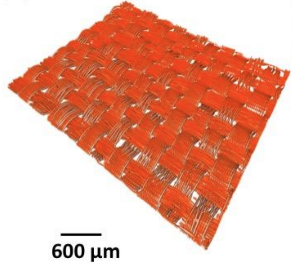
Figure 4: Microtomography of a parachute fabric (image credit: NASA/LBNL-Berkeley [28]).

(a) $2/7\times 2/7$

(b) $20\%\times 40\%$

(c) $10\%\times 80\%$

(d) $8\%\times 100\%$

Figure 5: Simple equivalent pore candidates with $\alpha=8\%$ but different aspect ratios: (a) 1:1; (b) 2:1; (c) 8:1; and (d) 12.5:1.

4.2 Exploration of candidate equivalent pores

The permeability of the PIA-C-7020 Type I fabric with Ripstop weave was measured and reported in [5]. A series of tests were conducted using a Textest Instruments FX 3300 Labotester III Air Permeability Tester, which consists of a test chamber with a vacuum pump. In all tests, the fabric sample was clamped over the test head opening and the upstream flow pressure was set to $p=94,625\ \mathrm{Pa}$. The temperature of the laboratory where the experiment was conducted was measured to be $T=296.5\ \mathrm{K}$ and the following air properties were assumed

$$\gamma=1.4,\quad R=287.2\ \mathrm{J\ kg^{-1}K^{-1}},\quad\textrm{and}\quad\mu=1.846\times 10^{-5}\ \mathrm{kg\ m^{-1}s^{-1}}.$$ (31)

Each different test was performed using still air and a different downstream pressure value that was maintained constant in time using the vacuum pump in the chamber. Then, the permeability of the fabric material was deduced from the experimentally obtained variation of the averaged velocity of the fluid through the fabric with the prescribed difference between the upstream and downstream pressure values.

For each candidate equivalent pore shown in Fig. 5, seven pore-resolved, unsteady numerical simulations mimicking the experimental setup described above are performed using direct numerical simulation (DNS) flow solver Hydrodynamics Adaptive Mesh Refinement Simulator (HAMeRS) [41] as described in Appendix B. In all simulations, the computational fluid domain is chosen to be the $4\ \mathrm{mm}\times 0.5\ \mathrm{mm}\times 0.5\ \mathrm{mm}$ box (dimensions in the $x$-, $y$-, and $z$-directions, respectively) shown in Fig. 1. The upstream (inlet) boundary conditions as well as the initial conditions in the half domain delimited in the $x$-direction by the inlet boundary and the porous wall are set to the uniform flow field defined by $\rho^{\textrm{up}}=1.111\ \mathrm{kg/m}^{3}$, ${\bm{v}}^{\textrm{up}}=0\ \mathrm{m\ s^{-1}}$, and $p^{\textrm{up}}=94,625\ \mathrm{Pa}$. As for the downstream (outlet) boundary conditions and the initial conditions in the other half of the computational fluid domain, they are set in each case to the uniform flow field defined by $\rho^{\textrm{dn}}=1.112\ \mathrm{kg/m}^{3}$ ($1.109\ \mathrm{kg/m}^{3}$, $1.105\ \mathrm{kg/m}^{3}$, $1.099\ \mathrm{kg/m}^{3}$, $1.088\ \mathrm{kg/m}^{3}$, $1.076\ \mathrm{kg/m}^{3}$, and $1.064\mathrm{kg/m}^{3}$), ${\bm{v}}^{\textrm{dn}}=0\ \mathrm{m\ s^{-1}}$, and $p^{\textrm{dn}}=94,525\ \mathrm{Pa}$ ($94,425\ \mathrm{Pa}$, $94,125\ \mathrm{Pa}$, $93,625\ \mathrm{Pa}$, $92,625\ \mathrm{Pa}$, $91,625\ \mathrm{Pa}$, and $90,625\mathrm{Pa}$). Note that these initial conditions are consistent with the temperature $T=296.5\ \mathrm{K}$ of the quiescent air in the laboratory.

At the beginning of each pore-resolved, unsteady numerical simulation characterized by a different uniform outlet pressure field, pressure waves propagate in both directions away from the porous fabric coupon. For each explored pore geometry, the pressure difference across the porous wall instantly drops, the fluid flow near the porous wall accelerates, and a weak jet stream forms downstream. In Fig. 6, the reader can observe that the computed Mach number profiles substantially differ across the considered pore geometries. As expected, the holes with the smaller aspect ratios ($2/7\times 2/7\textrm{ and }20\%\times 40\%$) lead to larger maximum Mach number values (around 0.2), which is consistent with the observation made in Section 3.3 that equivalent pores with smaller aspect ratios lead to smaller momentum dissipation.

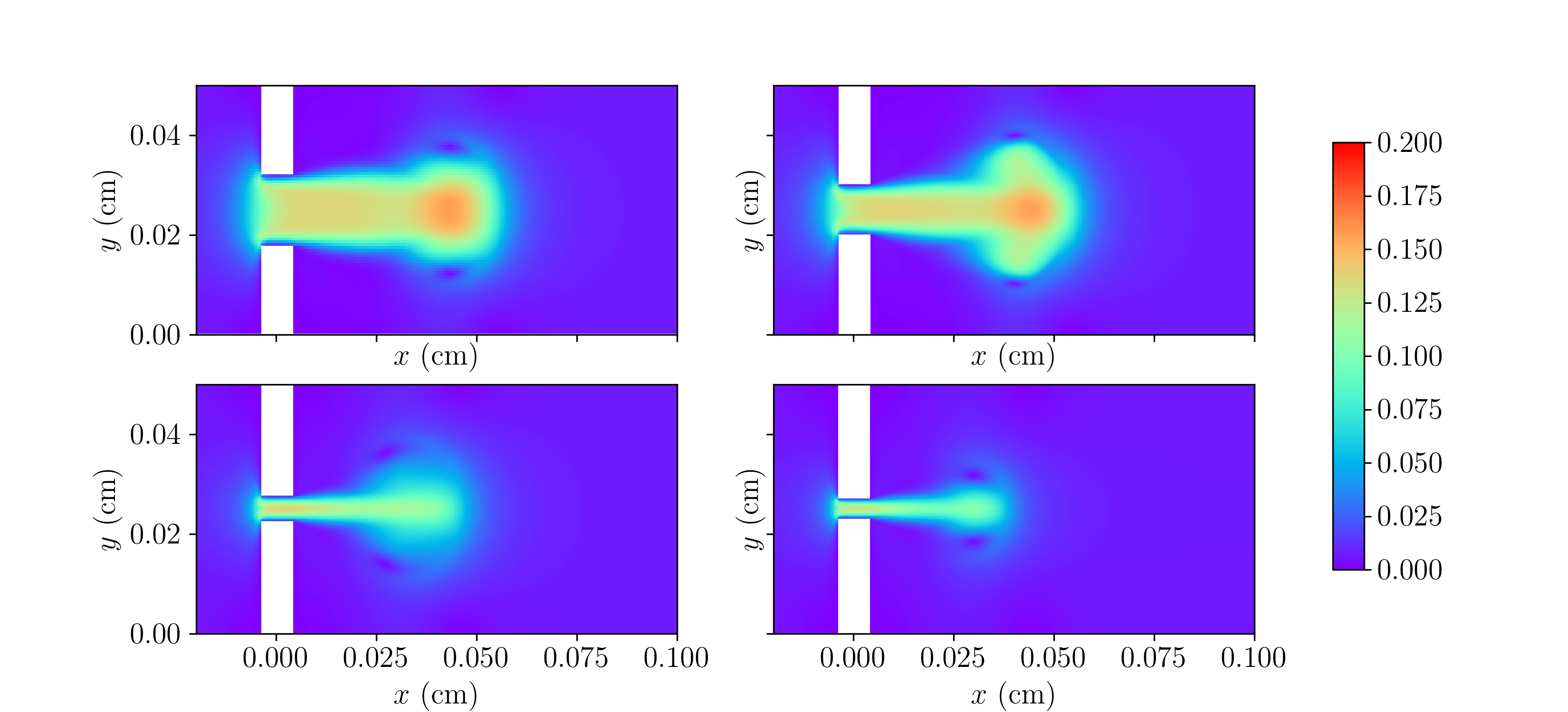
Figure 6: Mach number profiles in the central $x$-$y$ plane computed using pore-resolved numerical simulations and different pore geometries: $2/7\times 2/7$ (top-left); $20\%\times 40\%$ (top-right); $10\%\times 80\%$ (bottom-left); and $8\%\times 100\%$ (bottom-right) ($p^{up}-p^{dn}=3,000\ \mathrm{Pa}$, $t=15.8\ \mathrm{\mu s}$).

In each of the 28 performed pore-resolved numerical simulations, the pressure difference across the porous wall rapidly tends to become quasi-steady and the velocity field on each side of the porous wall converges to a steady-state value around $t=15.8\ \mathrm{\mu s}$. These results are reported in Fig. 7 in the form of velocity-pressure difference curves together with their counterpart experimental values measured in [5] within a confidence interval of $99.7\%$. Here, velocity refers to the averaged quasi-steady velocity through the fabric and pressure difference refers to the averaged quasi-steady pressure difference between both sides of the porous wall.

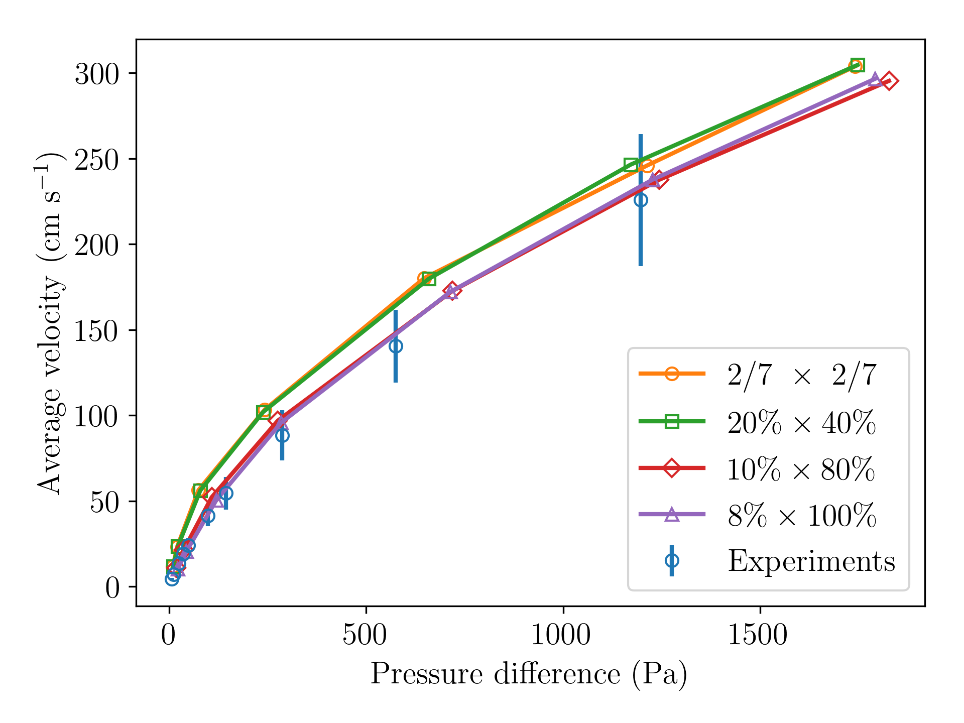
Figure 7: Permeability results (PIA-C-7020 Type I fabric with Ripstop weave): experimental data (blue circles and 99.7% confidence interval); and quasi-steady results of pore-resolved, unsteady numerical simulations (other symbols).

The permeability velocity through the porous membrane $u^{\textrm{pe}}$ is defined as the ratio of the averaged mass flux across $\Omega$ and the initial upstream density $\rho^{\textrm{up}}$ – that is,

$$u^{\textrm{pe}}=\displaystyle{\frac{\int_{\Omega}\rho u\,d\Omega}{|\Omega|\rho^{\textrm{up}}}}\,.$$ (32)

Both experimental and numerical results reported above are close to the incompressible flow regime, where the density fluctuation can be neglected. Indeed, all performed pore-resolved numerical simulations reveal a density fluctuation of the order of $2\%$. In this case, the definition (32) simplifies to $u^{\textrm{pe}}=\bar{u}$. From this result and Fig. 7, it follows that: each explored pore geometry leads to a numerical prediction of the permeability velocity that matches reasonably well its experimentally measured counterpart; but the geometry labeled as (d) in Fig. 5, which is characterized by the highest aspect ratio ($8\%\times 100\%$ or 12.5:1) , delivers the closest permeability velocity value to the experimentally measured one and therefore is the most suitable equivalent pore geometry.

It is worth noting that according to [6] and for a given wall permeability, the total pressure drop across a porous wall $(\Delta p)^{\textrm{tot}}$ can be split into two components due to viscous and inertial effects – that is,

$$\Delta p^{\textrm{tot}}=\Delta p^{\textrm{vis}}+\Delta p^{\textrm{ine}}.$$ (33)

The viscous effect is dominant at low Reynolds number and the inertial effect prevails at high Reynolds number. The study carried out herein falls into the former category ($10\leq Re\leq 400$), where one contribution of the viscous effect is the friction loss due to the shear stress near the surface of each spun fiber. Pore geometries characterized by smaller aspect ratios (e.g., $2/7\times 2/7$ and $20\%\times 40\%$) are also characterized by smaller pore surfaces (e.g., see Fig. 5): hence, they lead to smaller values of $\Delta p^{\textrm{vis}}$ and therefore smaller values of $\Delta p^{\textrm{tot}}$. This explains why the pore geometries with the larger aspect ratios (e.g., $10\%\times 80\%$ and $8\%\times 100\%$) are found in Fig. 7 to lead to numerical predictions of the permeability velocity that match better the experimental data.

4.3 Verification for a supersonic application

Here, the homogenization approach presented in this paper is verified for a series of supersonic instances of the porous flow model problem graphically depicted in Fig. 1. In each instance:

• The computational fluid domain is chosen to be the $10\ \mathrm{mm}\times 0.5\ \mathrm{mm}\times 0.5\ \mathrm{mm}$ box (dimensions in the $x$-, $y$-, and $z$-directions, respectively).

• This domain is divided in two non overlapping subdomains labeled as “Upstream” and “Downstream”: the interface $\Gamma$ between them is located at $250\ \mathrm{\mu m}$ from the porous wall within the Upstream subdomain (see Fig. 8 below).

  Figure 8: Supersonic porous flow model problem: separation of the computational fluid domain in two subdomains; interface $\Gamma$; and initial shock (central $x$-$y$ plane view).

• In both subdomains, the flow solution is initialized using constant states chosen so that at $t=0$, a shock occurs at $x=\Gamma$ with a specified initial speed $V_{s}$. Specifically:

  • In the Upstream subdomain, the flow solution is initialized as follows

    $$\rho^{\textrm{up}}(x,y,z,0) = 0.0076\ \mathrm{kg\ m^{-3}}\,,\quad p^{\textrm{up}}(x,y,z,0)=260\ \mathrm{Pa}\,,$$

    $$u^{\textrm{up}}(x,y,z,0) = u^{\textrm{up}}(V_{s},\textrm{RH})\,,\quad{\textrm{and}}\quad v(x,y,z,0)=w(x,y,z,0)=0\,,$$

    where the notation $\spadesuit(V_{s},\textrm{RH})$ designates that $\spadesuit$ is determined from $V_{s}$ and the Ranking-Hugoniot jump conditions.

  • In the Downstream subdomain, the flow is assumed to be initially quiescent and in a constant state determined by $V_{s}$ and the Rankine-Hugoniot jump conditions (see Tab. 1) – that is

    $$\rho^{\textrm{dn}}(x,y,z,0) = \rho^{\textrm{dn}}(V_{s},\textrm{RH})\,,\quad p^{\textrm{dn}}(x,y,z,0)=p^{\textrm{dn}}(V_{s},\textrm{RH})\,,$$

    $$\textrm{and}\quad u^{\textrm{dn}}(x,y,z,0) = v(x,y,z,0)=w(x,y,z,0)=0.$$

  • The Mars atmosphere consisting mainly of carbon dioxide CO₂, the gas properties are set to

    $$\gamma=1.33,\quad R=188.4\ \mathrm{J\ kg^{-1}K^{-1}},\quad\textrm{and}\quad\mu=1.03\times 10^{-5}\ \mathrm{kg\ m^{-1}s^{-1}}.$$ (34)

• At each subdomain boundary facing $\Gamma$ – that is, at each of the inlet and outlet boundaries – the boundary conditions are set to the uniform flow defined by the constant state used to specify the initial conditions in that subdomain.

• Two equivalent pore geometries defined by the aspect ratios $2/7\times 2/7$ and $8\%\times 100\%$ ($\alpha=8\%$) are considered.

• For each considered equivalent pore geometry, three unsteady numerical simulations are performed in a time-interval sufficiently large to capture the reflection of the shock wave on the porous wall:

  • One three-dimensional pore-resolved simulation performed using DNS flow solver HAMeRS as described in Appendix B to generate reference data.

  • Two counterpart one-dimensional simulations performed using the flow solver AERO-F [10, 8] equipped with the EBM FIVER [38, 19, 22, 12] and the homogenization approach presented in this paper (see Appendix A): one simulation performed using 400 grid points; and one performed using 2,000 grid points.

Each aforementioned supersonic instance of the porous flow model problem graphically depicted in Fig. 1 is defined by a specified shock speed value $V_{s}$. Three different values of $V_{s}$ are considered: $V_{s}=279.4\ \mathrm{m\ s^{-1}}$, $V_{s}=335.9\ \mathrm{m\ s^{-1}}$, and $V_{s}=367.1\ \mathrm{m\ s^{-1}}$. In all cases, the effect of bulk viscosity is neglected.

$V_{s}$	Upstream boundary/initial conditions	Downstream boundary/initial conditions
$279.4\ \mathrm{m\ s^{-1}}$	$\rho=0.0076\ \mathrm{kg\ m^{-3}}$, $u=127.98\ \mathrm{m\ s^{-1}}$, $p=260\ \mathrm{Pa}$	$\rho=0.004119\ \mathrm{kg\ m^{-3}}$, $u=0\ \mathrm{m\ s^{-1}}$, $p=112.73\ \mathrm{Pa}$
$335.9\ \mathrm{m\ s^{-1}}$	$\rho=0.0076\ \mathrm{kg\ m^{-3}}$, $u=213.31\ \mathrm{m\ s^{-1}}$, $p=260\ \mathrm{Pa}$	$\rho=0.002774\ \mathrm{kg\ m^{-3}}$, $u=0\ \mathrm{m\ s^{-1}}$, $p=61.240\ \mathrm{Pa}$
$367.1\ \mathrm{m\ s^{-1}}$	$\rho=0.0076\ \mathrm{kg\ m^{-3}}$, $u=255.97\ \mathrm{m\ s^{-1}}$, $p=260\ \mathrm{Pa}$	$\rho=0.002300\ \mathrm{kg\ m^{-3}}$, $u=0\ \mathrm{m\ s^{-1}}$, $p=43.772\ \mathrm{Pa}$

Table 1: Supersonic porous flow model problem: boundary and initial conditions (additionally, $v=w=0\ \mathrm{m\ s^{-1}}$ in all cases and both subdomains).

4.3.1 Pore-resolved numerical simulations

For each considered pore geometry and each considered shock speed value $V_{s}$, the results of the pore-resolved, unsteady simulation reveal that when the shock bounces off the porous wall, a high density/high pressure flow zone develops upstream of the porous wall. Consequently, the flow through the pore behaves like a flow through a converging-diverging nozzle. Downstream of the porous wall, the flow immediately accelerates and goes through an expansion. Fig. 9 displays the Mach number profiles computed at $t=23.46\ \mathrm{\mu s}$. It shows that as in the case of low-speed flow (see Fig. 6), the pore geometry with the smaller aspect ratio leads to jet streams. However, the reader can also observe that in the high-speed case, the flows are choked.

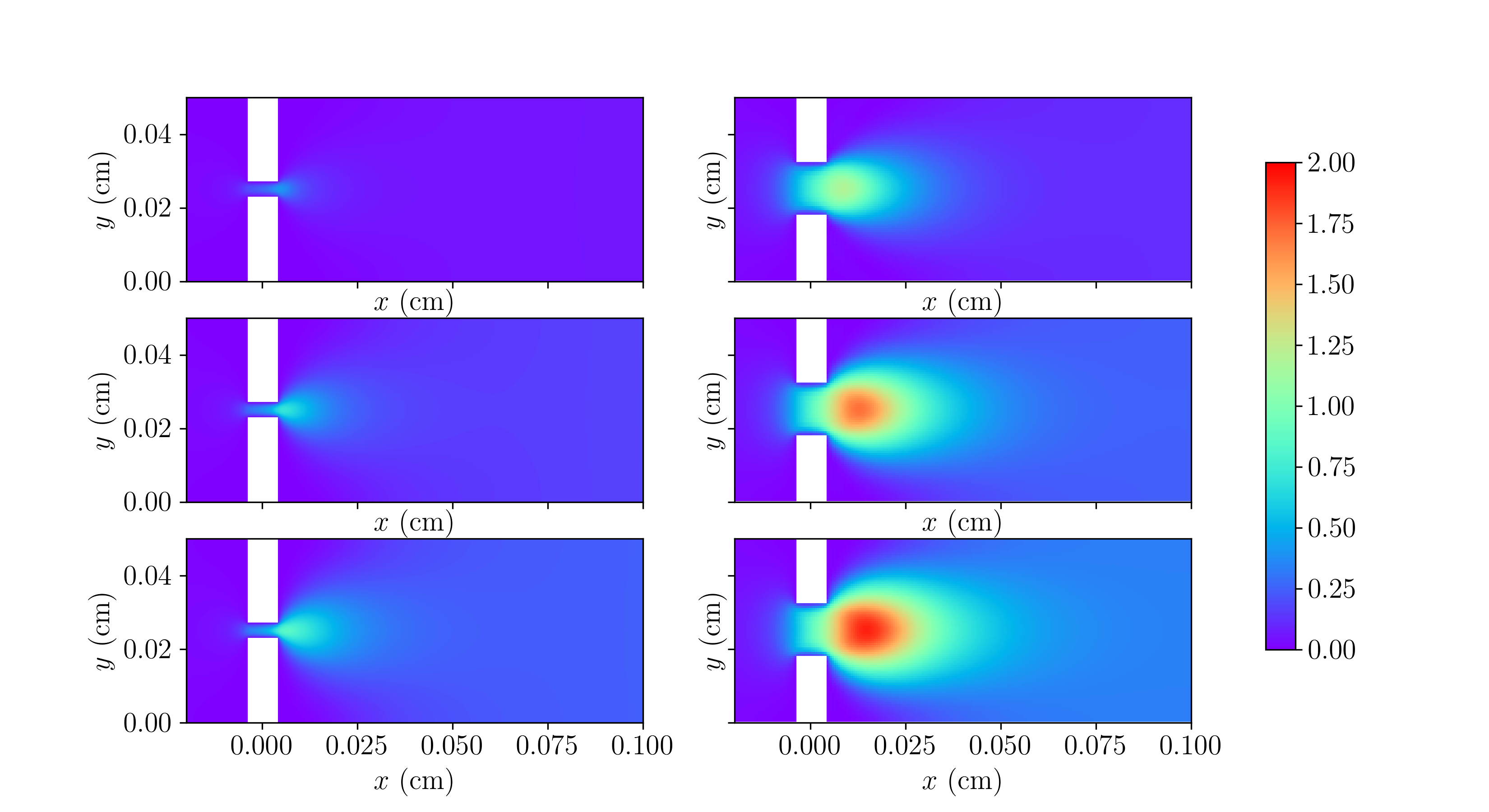
Figure 9: Mach number profiles in the central $x$-$y$ plane computed at $t=23.46\ \mathrm{\mu s}$ using pore-resolved, unsteady numerical simulations: pore geometry with $2/7\times 2/7$ aspect ratio (left) and $8/\%\times 100/\%$ aspect ratio (right); $V_{s}=279.4,\ 335.9,\ \textrm{and}\ 367.1\ \mathrm{m\ s^{-1}}$ (top to bottom).

Let

$$Re=\displaystyle{\left(\frac{\int_{\Omega^{\textrm{pore}}}\rho u^{2}\,d\Omega^{\textrm{pore}}}{\rho^{\textrm{up}}|\Omega^{\textrm{pore}}|}\right)^{1/2}\frac{\rho^{\textrm{up}}d}{\mu}},$$ (35)

where $|\Omega^{\textrm{pore}}|$ denotes the area of the pore and $d=\sqrt{4|\Omega^{\textrm{pore}}|/\pi}$ is the pore diameter, denote the Reynolds number based on the jet flow velocity at the pore exit. Tab. 2 reports the values of this number computed at $t=23.46\ \mathrm{\mu s}$ by post-processing the results of the pore-resolved simulations. The reported low values, which are partially due to the low density and partially to the small pore size, highlight the importance of accounting for viscous effects when computing flows past porous walls

Aspect ratio of pore geometry	$V_{s}=279.4\ \mathrm{m\ s^{-1}}$	$V_{s}=335.9\ \mathrm{m\ s^{-1}}$	$V_{s}=367.1\ \mathrm{m\ s^{-1}}$
$2/7\times 2/7$	7.3	13.50	17.96
$8\%\times 100\%$	16.43	23.75	27.38

Table 2: Reynolds numbers based on the jet flow velocity computed at $t=23.46\ \mathrm{\mu s}$ using pore-resolved numerical simulations.

Fig. 10 reports for each considered pore geometry the variation of the averaged mass flow rate with the pressure difference between both sides of the porous wall computed by post-processing at each time-step of the computation the results of the corresponding pore-resolved, unsteady numerical simulation. Each variation is found to be linear and therefore describable by

$$\overline{\rho u}\approx K\overline{\Delta p}.$$ (36)

In other words, it satisfies Darcy’s law, where the constant $K$ depends on the pore geometry. In this case, a simple least square fitting yields $K=1.61\times 10^{-4}\ \mathrm{s\ m^{-1}}$ for the pore geometry with $2/7\times 2/7$ aspect ratio and $K=8.54\times 10^{-5}\ \mathrm{s\ m^{-1}}$ for that with $8\%\times 100\%$ aspect ratio.

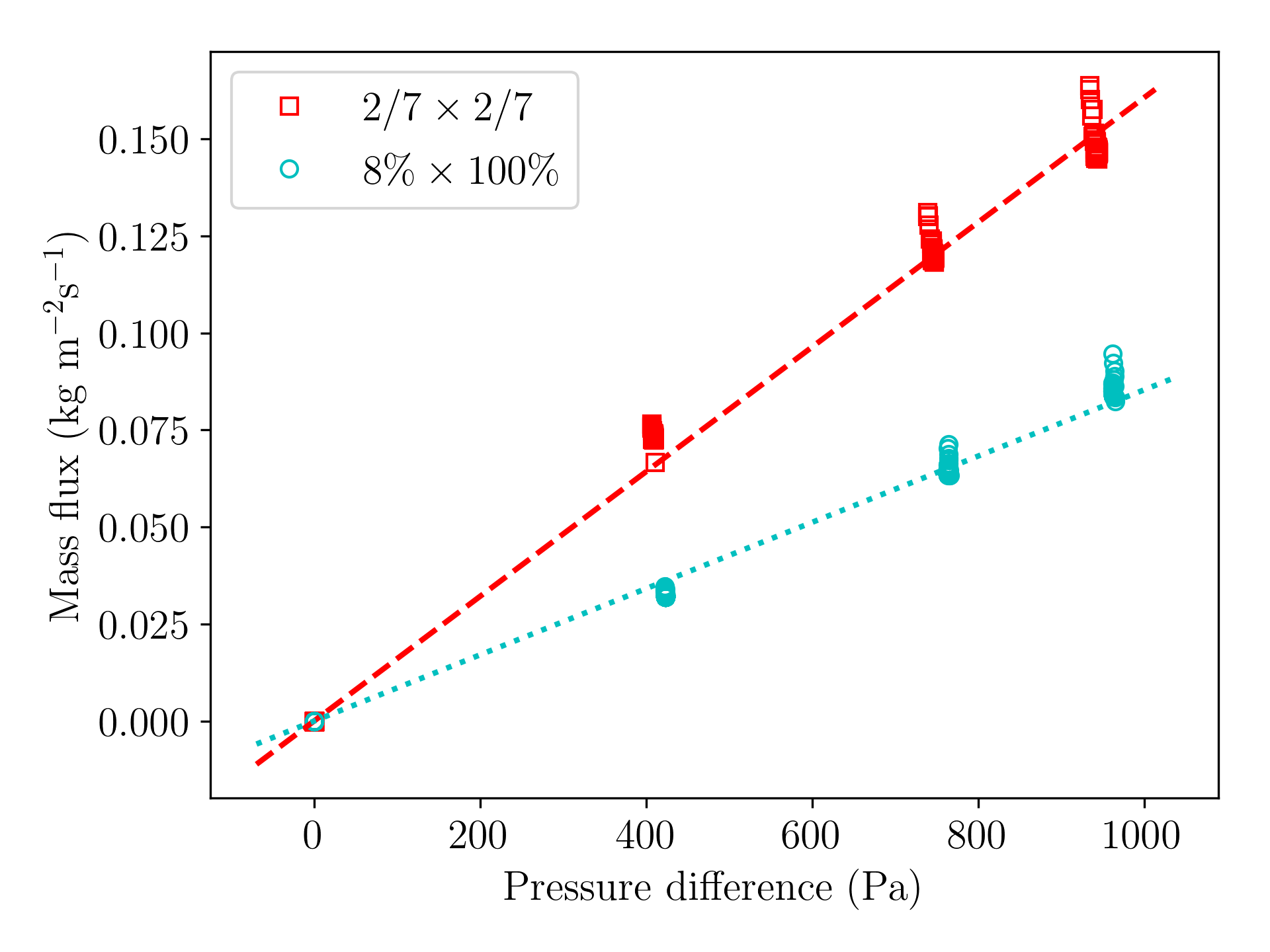
Figure 10: Variations of the averaged mass flow rate with the pressure difference computed using pore-resolved, unsteady numerical simulations.

4.3.2 Homogenization-based numerical simulations

Recall that all numerical simulations discussed herein are performed at the coupon level, due to the periodicity of the weave pattern (see Section 4.1). For this reason and due to the flat geometry of the considered porous wall (see Fig. 8), all counterparts of the pore-resolved, unsteady numerical simulations presented in Section 4.3.1 based on the homogenization approach described in this paper are performed in one dimension, in the computational fluid domain $x\in[-0.5,0.5]\ \mathrm{cm}$. Two discretizations of this domain in dual computational cells are considered for this purpose: one with $N=400$ grid points; and one with $N=2,000$ grid points. In each case, the porous wall is “embedded” in the discretization at $x=0$. The homogenization-based numerical simulations are performed using the vertex-based, finite volume flow solver AERO-F [10, 8] equipped with the second-order space-accurate EBM FIVER [22] (see also Appendix A) and the second-order explicit Runge-Kutta time-integrator constrained by the constant CFL number of 0.5.

Because for the equivalent pore with the aspect ratio of $2/7\times 2/7$ the jet stream was reported in Section 4.3.1 to expand immediately downstream of the porous wall (see Fig. 9), the thickness correction factor (see Section 3.3) is set for this case to $\eta_{f}=1$. For the equivalent pore with the aspect ratio of $8\%\times 100\%$, the jet stream can be seen in Fig. 9 to extend further in the computational fluid domain: thus, the thickness correction factor is set in this case to $\eta_{f}=4$.

Figs. 11, 12 and 13 report the averaged density, streamwise velocity, and pressure profiles computed at $t=23.46\ \mathrm{\mu s}$ using the proposed homogenization approach. It shows that: the one-dimensional discretization of $[-0.5,0.5]\ \mathrm{cm}$ in $N=400$ grid points is well resolved; and the results obtained using the proposed homogenization approach agree well with their counterparts obtained using the pore-resolved numerical simulations.

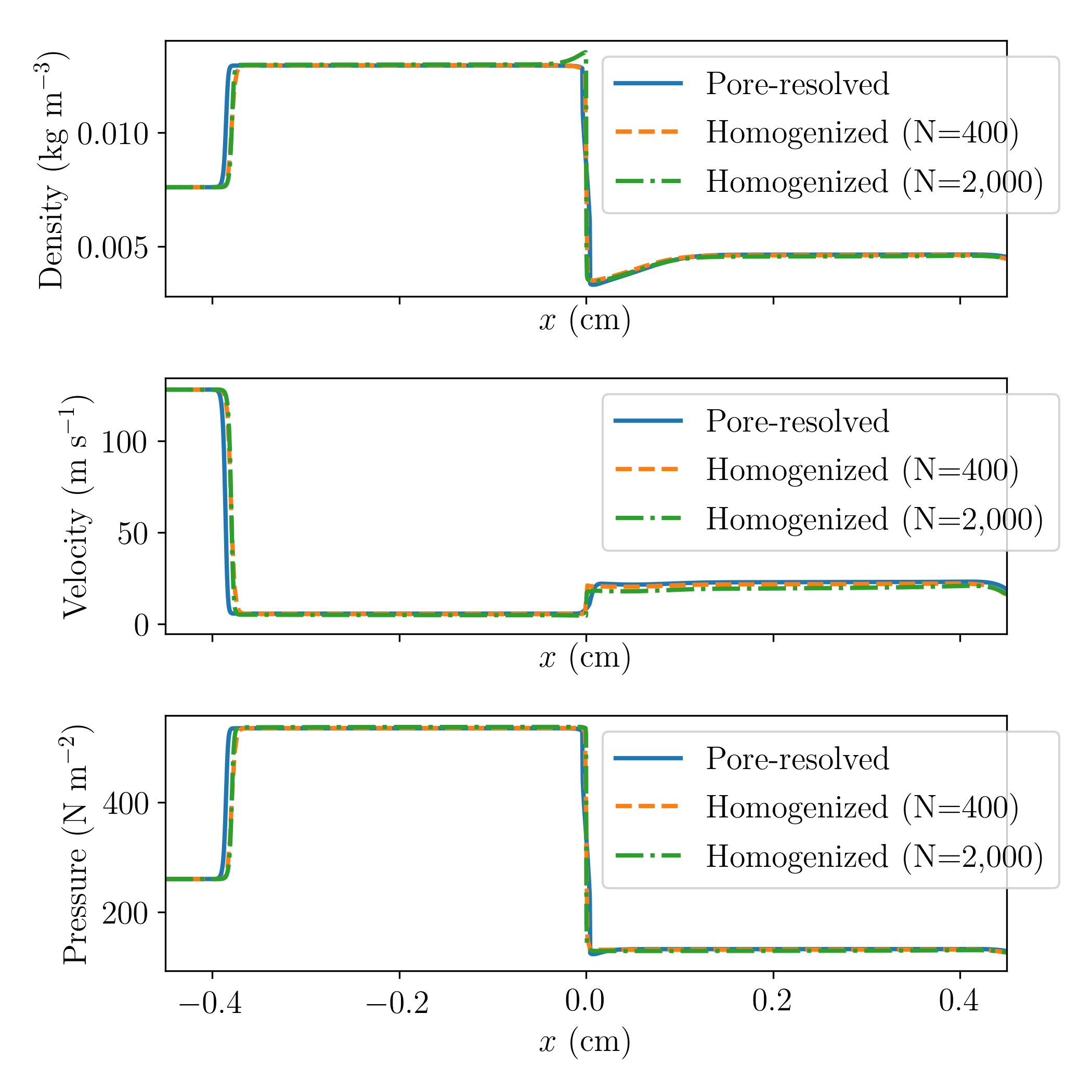
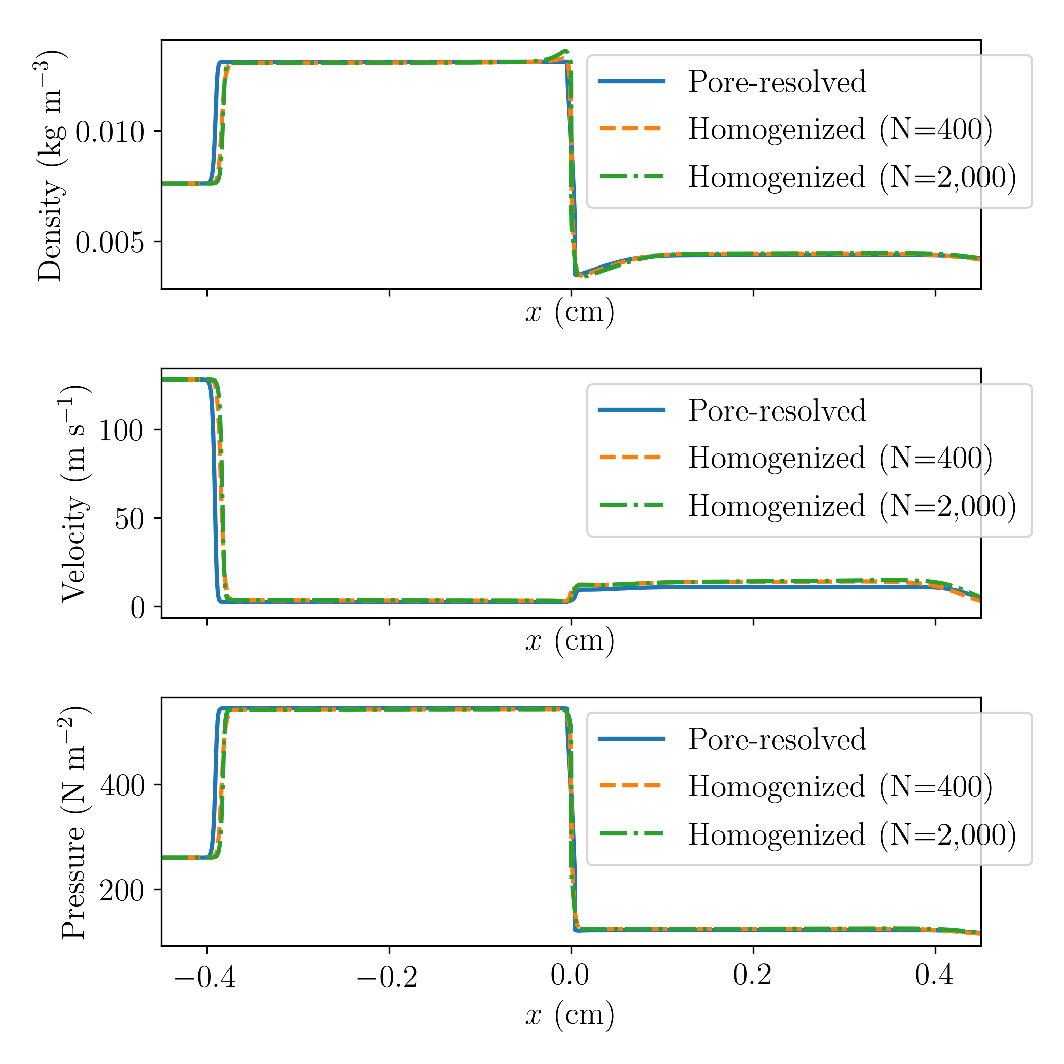
Figure 11: Averaged density, streamwise velocity, and pressure profiles (top to bottom) predicted at $t=23.46\ \mathrm{\mu s}$ for $V_{s}=279.4\mathrm{m\ s^{-1}}$: pore with aspect ratio of $2/7\times 2/7$ (left); and pore with aspect ratio of $8\%\times 100\%$ (right).

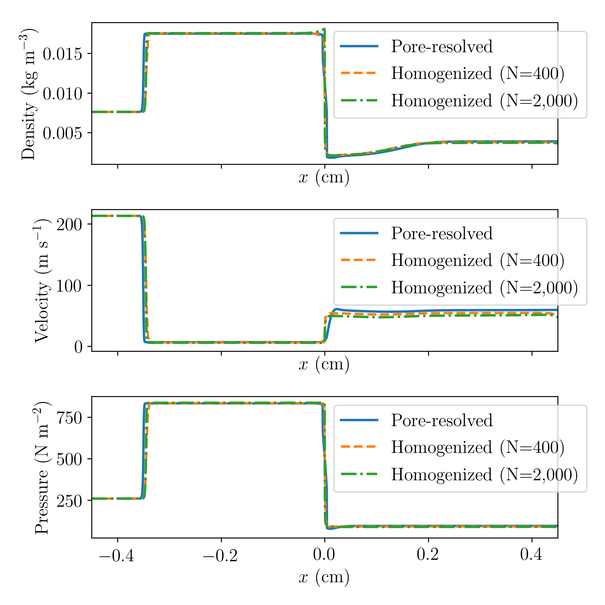
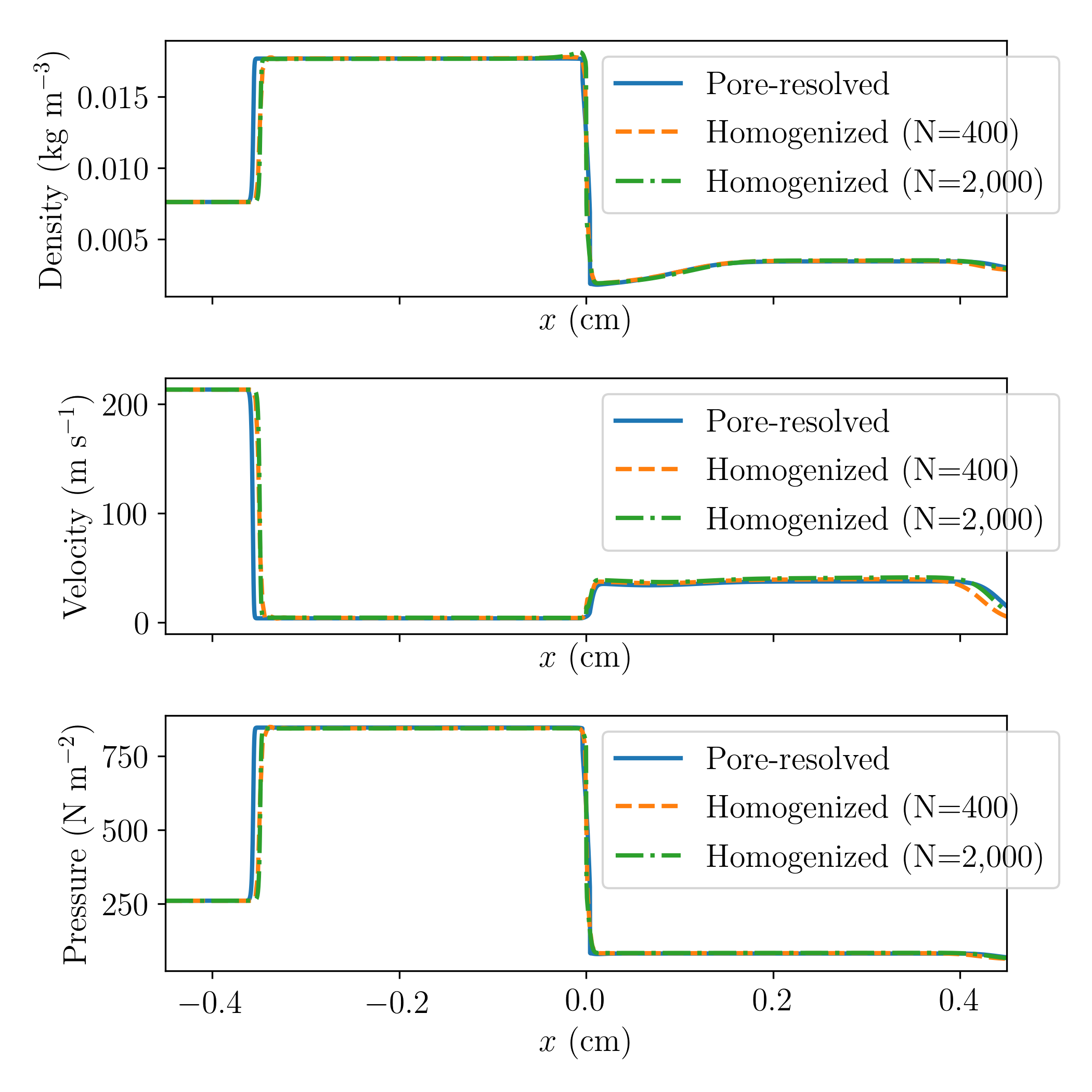
Figure 12: Averaged density, streamwise velocity, and pressure profiles (top to bottom) predicted at $t=23.46\ \mathrm{\mu s}$ for $V_{s}=335.9\mathrm{m\ s^{-1}}$: pore with aspect ratio of $2/7\times 2/7$ (left); and pore with aspect ratio of $8\%\times 100\%$ (right).

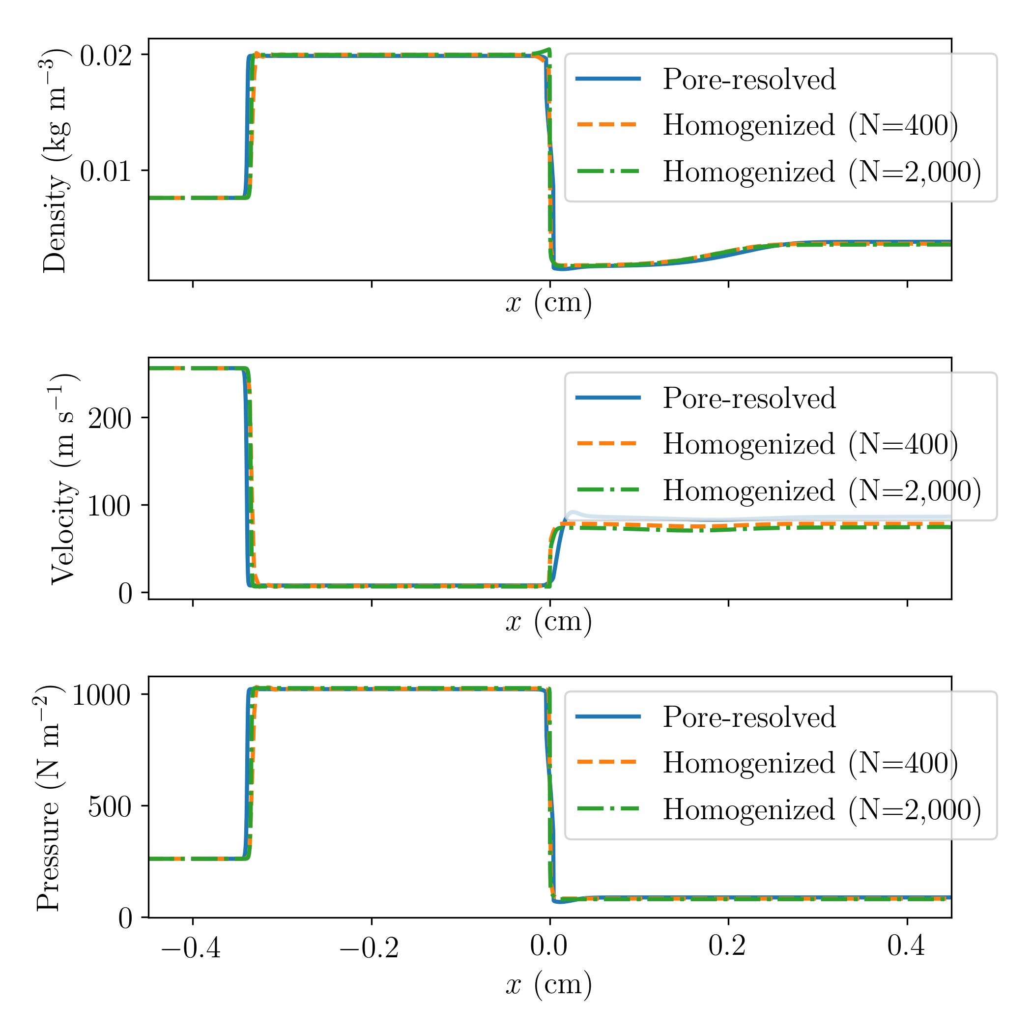
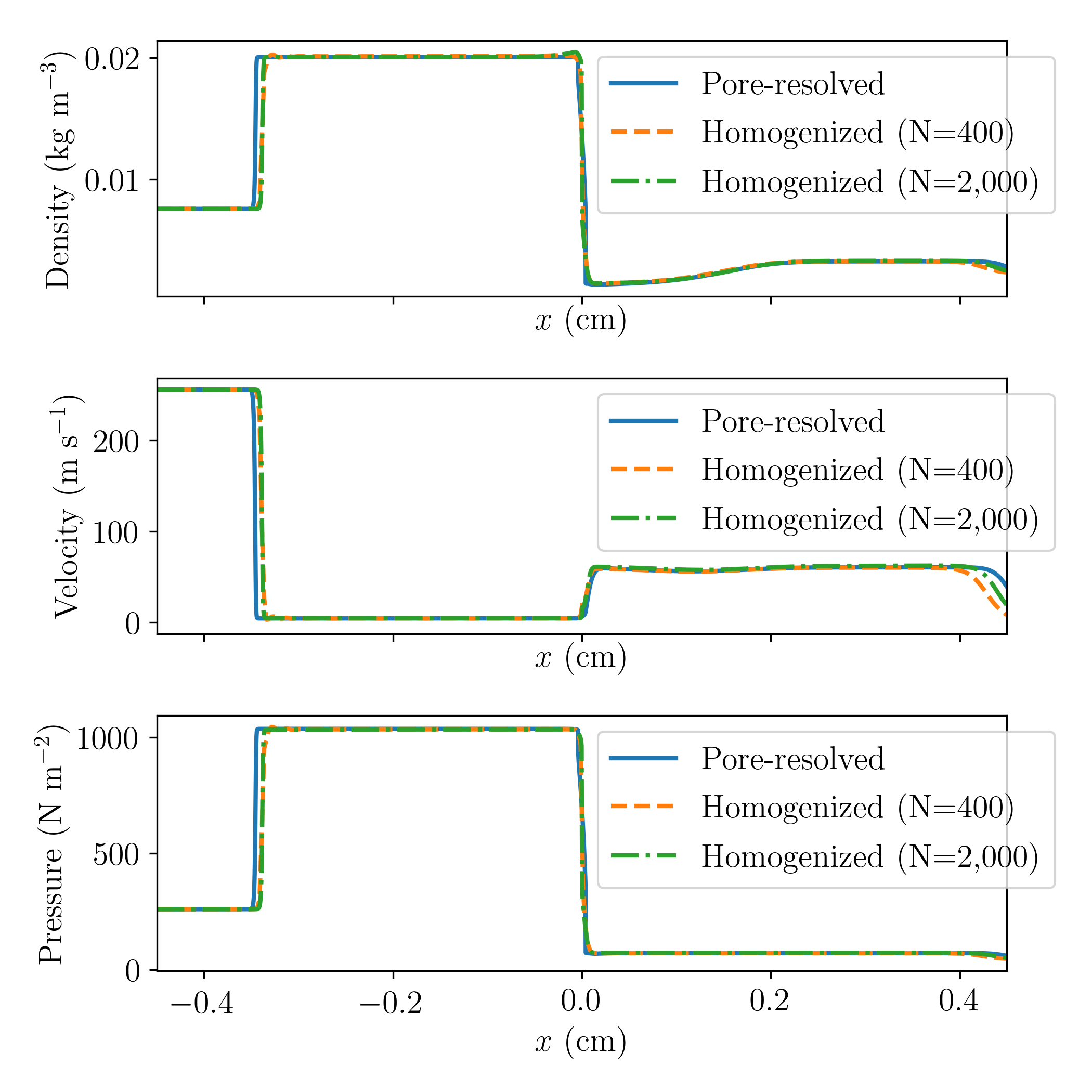
Figure 13: Averaged density, streamwise velocity, and pressure profiles (top to bottom) predicted at $t=23.46\ \mathrm{\mu s}$ for $V_{s}=367.1\mathrm{m\ s^{-1}}$: pore with aspect ratio of $2/7\times 2/7$ (left); and pore with aspect ratio of $8\%\times 100\%$ (right).

Next, attention is focused on the drag force $F_{D}$ generated by the porous wall. For a pore-resolved numerical simulation, $F_{D}$ can be defined as

$$F_{D}=\underbrace{-\int_{\partial{\Omega_{\textrm{vol}}}\backslash\partial\Omega_{\textrm{vol}}^{\textrm{pore}}}pn\ d\partial\Omega_{\textrm{vol}}}_{<1>}+\underbrace{\int_{\partial{\Omega_{\textrm{vol}}}\backslash\partial\Omega_{\textrm{vol}}^{\textrm{pore}}}\uptau\cdot n\ d\partial\Omega_{\textrm{vol}}}_{<2>}+\underbrace{\int_{\partial\Omega_{\textrm{vol}}^{\textrm{pore}}}\uptau\cdot n\ d\partial\Omega_{\textrm{vol}}^{\textrm{pore}}}_{<3>},$$ (37)

where $\Omega_{\textrm{vol}}$ denotes the volume representation of the porous wall, $\Omega_{\textrm{vol}}^{\textrm{pore}}$ denotes the part of $\Omega_{\textrm{vol}}$ occupied by the pores, $\partial{\Omega_{\textrm{vol}}}$ denotes the wet boundary surface of $\Omega_{\textrm{vol}}$, $\partial\Omega_{\textrm{vol}}^{\textrm{pore}}$ denotes the boundary surface of $\Omega_{\textrm{vol}}^{\textrm{pore}}$, and $n$ denotes the unit, outward normal to the surface over which the spatial integration is performed. Hence, $F_{D}$ consists in this case of a force due to the pressure jump across the porous wall (term ¡1¿ in (37)), a force induced by the jump of the normal component of the shear stress traction across the porous wall (term ¡2¿ in (37)), and the shear force on the pore boundaries (term ¡3¿ in (37)).

For a simulation based on the homogenization approach proposed in this paper, $F_{D}$ can be defined consistently with (37) as follows

$$F_{D}=-\int_{\Omega}pn\ d\partial\Omega+\int_{\Omega}\tau\cdot n\ d\partial\Omega\,,$$ (38)

which in the case of the one-dimensional homogenized computations performed herein simplifies to

$$F_{D}=-\int_{\Omega}pn\ d\partial\Omega+\int_{\Omega}\tau\cdot n\ d\partial\Omega=|\Omega|(\Delta p^{\textrm{tot}}-\Delta{\uptau}_{xx})|\Omega|.$$ (39)

Each of the integrals in (37) and (39) can be evaluated numerically using standard approximations. In the context of an EBM for CFD, the load evaluation algorithm presented in [19] can be used for this purpose.

Fig. 14 shows that for $N=400$, the homogenization-based numerical simulations accurately reproduce in all cases the variation with the shock speed of the drag force per unit area obtained at $t=23.46\ \mathrm{\mu s}$ using the counterpart pore-resolved numerical simulation.

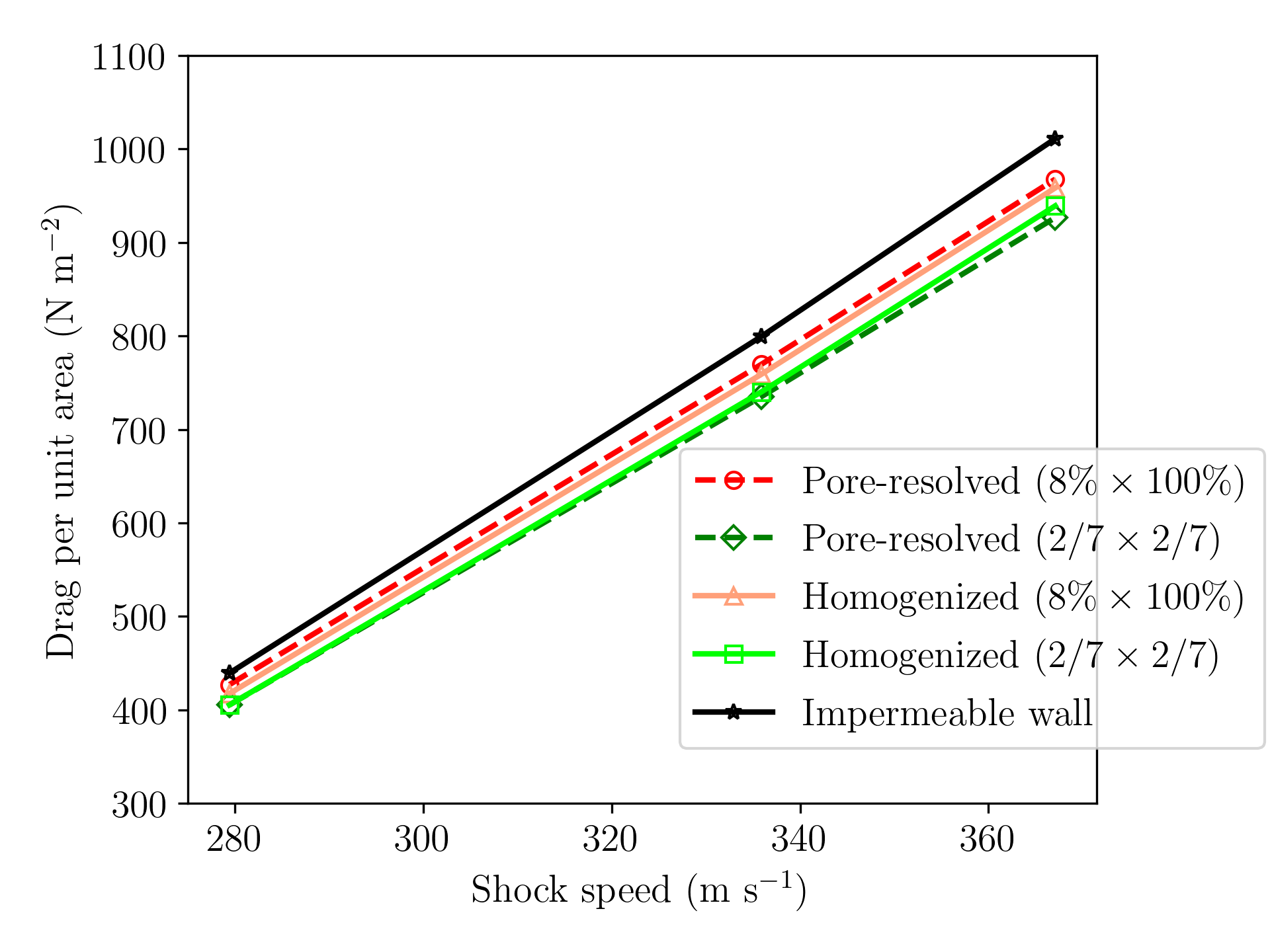
Figure 14: Variations with the shock speed of the drag force per unit area predicted at $t=23.46\ \mathrm{\mu s}$ (for homogenization-based numerical simulations, $N=400$).

5 Conclusions

The homogenization approach proposed in this paper for the treatment of porous wall boundary conditions distinguishes itself from alternatives in many ways. To begin, it is valid for both incompressible and compressible viscous flows. It does not require prescribing neither a mass flow rate nor a heuristic discharge coefficient. Instead, it models the inviscid flux through a porous wall surrounded by the flow as a weighted average of the inviscid flux at an impermeable surface and that through pores, and introduces a body force term in the governing equations to account for friction loss along the pore boundaries. The latter term is parameterized however by a thickness correction factor. The proposed approach, which can be implemented in any semi-discretization or discretization method, is successfully verified for a series of one-dimensional supersonic flow problems through a rigid porous wall, using three-dimensional pore-resolved numerical simulations. Its successful application to three-dimensional fluid-structure interaction problems associated with supersonic parachute inflation dynamics during Mars landing is reported in the companion papers  [14, 2].

Appendix A EBM FIVER and arbitrary embedding CFD meshes

Brief descriptions of the simplest version of the FInite Volume method with Exact two-material Riemann problems (FIVER) [38] and the implementation in this Embedded Boundary Method (EBM) for CFD of the proposed homogenization approach for the treatment of porous wall boundary conditions are provided here, in the context of arbitrary embedding CFD meshes. For more advanced versions of FIVER, the reader is referred to, for example, [22, 12, 4].

FIVER semi-discretizes the inviscid fluxes of Eq. 1 by a vertex-based Finite Volume (FV) method and the viscous fluxes of this equation by a FE method. Both methods are known for their ability to operate on arbitrary meshes. Using the standard characteristic function associated with a control volume (dual cell) $\mathcal{C}_{i}$ defined at a grid point $i$ of the structured or arbitrarily unstructured CFD mesh, the standard piecewise-linear tent test function $\psi_{i}$ associated with the grid point $i$, the standard bijection between the space of piecewise linear FE functions defined over the primal elements of the CFD mesh and the space of constant characteristic shape functions defined over the dual cells of this mesh [7], FIVER adopts the standard variational approach and integration by parts to semi-discretize Eq. 1 as follows

$${|\mathcal{C}_{i}|\dfrac{\partial\bm{W}_{i}}{\partial t}}+\sum_{j\in\mathcal{K}(i)}\int_{\partial\mathcal{C}_{ij}}\mathcal{F}(\bm{W}_{h})\bm{\cdot}n_{ij}\,d\partial B\,+\int_{\partial\mathcal{C}_{i}\cap\partial B_{\infty}}\mathcal{F}(\bm{W}_{h})\bm{\cdot}n_{\infty}\,d\partial B\,+\sum_{B^{e}\ni\,i}\int_{B^{e}}\nabla{\psi^{e}_{i}}\bm{\cdot}\mathcal{G}(\bm{W}_{h})\,dB^{e}\,=0.$$ (40)

In Eq. 40 above, $|\mathcal{C}_{i}|$ denotes the volume of $\mathcal{C}_{i}$, $\partial\mathcal{C}_{i}$ denotes its boundary, $\partial\mathcal{C}_{ij}$ denotes the cell facet shared by $\mathcal{C}_{i}$ and $\mathcal{C}_{j}$, $n_{ij}$ denotes the unit outward normal to $\partial\mathcal{C}_{ij}$, $\bm{W}_{h}$ denotes the spatial approximation of the fluid state vector $\bm{W}$, $\bm{W}_{i}$ denotes the average value of $\bm{W}_{h}$ in $\mathcal{C}_{i}$, $\mathcal{K}(i)$ denotes the set of grid points connected by an edge to the grid point $i$, $B$ denotes the computational fluid domain and $\partial B_{\infty}$ denotes its far-field boundary, $n_{\infty}$ denotes the unit outward normal to $\partial B_{\infty}$, $B^{e}$ denotes a primal element of the CFD mesh discretizing $B$, and $\psi^{e}_{i}$ denotes the restriction of $\psi_{i}$ to $B^{e}$.

Let $\Omega$ denote a surface embedded in the discretization of $B$ by a CFD mesh and let $(i,j)$ be an edge of this mesh that intersects $\Omega$ (see Fig. 15). In order to semi-discretize the inviscid flux through $\partial\mathcal{C}_{ij}$, the simplest version of FIVER assumes that the midpoint $M$ of the edge $(i,j)$ lies on $\Omega$ – and more specifically, $\partial\mathcal{C}_{ij}$ lies on $\Omega$; constructs a fluid-structure half-Riemann problem at the point $M$ in the direction of the normal $n_{ij}$ to $\partial\mathcal{C}_{ij}$; solves this half-Riemann problem to obtain the fluid state vector at the point $M$, $\bm{W}_{i}^{\star}$; and then approximates the inviscid flux through $\partial\mathcal{C}_{ij}$ as follows

$$\int_{\partial\mathcal{C}_{ij}}\mathcal{F}(\bm{W}_{h})\bm{\cdot}n_{ij}\,dB \approx \bm{F}_{ij}=|\partial\mathcal{C}_{ij}|\,\bm{F}^{\textrm{{Roe}}}(\bm{W}_{i},\bm{W}_{i}^{\star},n_{ij}),\quad\textrm{if the grid point}~{}i~{}\textrm{lies in}~{}B$$

and (41)

$$\int_{\partial\mathcal{C}_{ji}}\mathcal{F}(\bm{W}_{h})\bm{\cdot}n_{ji}\,dB \approx \bm{F}_{ji}=|\partial\mathcal{C}_{ji}|\,\bm{F}^{\textrm{{Roe}}}(\bm{W}_{j},\bm{W}_{j}^{\star},n_{ji}),\quad\textrm{if the grid point}~{}j~{}\textrm{lies in}~{}B,$$

where $|\partial\mathcal{C}_{ij}|$ = $|\partial\mathcal{C}_{ji}|$ and $n_{ji}=-n_{ij}$. Note that by computing $\bm{W}_{i}^{\star}$ (or $\bm{W}_{j}^{\star}$) via the solution of a fluid-structure half-Riemann problem, FIVER is able to capture any shock or rarefaction wave near the embedded surface – that is, at the fluid-structure interface. Away from $\Omega$ – that is, when the edge $(i,j)$ does not intersect $\Omega$, FIVER approximates the inviscid flux through $\partial\mathcal{C}_{ij}$ using a standard FV method based on a standard approximate Riemann solver.

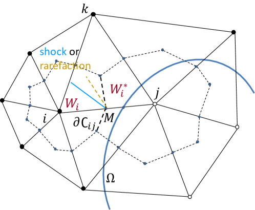
Figure 15: Embedding of a porous wall $\Omega$ in a CFD mesh: construction and solution of a fluid-structure half-Riemann problem at the midpoint $M$ of the edge $(i,j)$ intersecting $\Omega$.

From (41) and Eq. 15, it follows that if $\Omega$ is a porous wall, the homogenized, numerical inviscid flux functions through $\Omega$ can be computed by FIVER as follows

$$\begin{split}\bm{F}^{\textrm{ave}}_{ij}&=|\partial{\mathcal{C}}_{ij}|\left(\alpha\bm{F}^{\textrm{{Roe}}}(\overline{\bm{W}}_{i},\overline{\bm{W}}_{j},n_{ij})+(1-\alpha)\bm{F}^{\textrm{imp-wall}}(\overline{\bm{W}}_{i},n_{ij})\right)=|\partial{\mathcal{C}}_{ij}|\left(\alpha\bm{F}^{\textrm{{Roe}}}(\overline{\bm{W}}_{i},\overline{\bm{W}}_{j},n_{ij})+(1-\alpha)\bm{F}^{\textrm{{Roe}}}(\bm{W}_{i},\bm{W}_{i}^{\star},n_{ij})\right)\,,\\ \bm{F}^{\textrm{ave}}_{ji}&=|\partial{\mathcal{C}}_{ji}|\left(\alpha\bm{F}^{\textrm{{Roe}}}(\overline{\bm{W}}_{j},\overline{\bm{W}}_{i},n_{ji})+(1-\alpha)\bm{F}^{\textrm{imp-wall}}(\overline{\bm{W}}_{j},n_{ji})\right)=|\partial{\mathcal{C}}_{ji}|\left(\alpha\bm{F}^{\textrm{{Roe}}}(\overline{\bm{W}}_{j},\overline{\bm{W}}_{i},n_{ji})+(1-\alpha)\bm{F}^{\textrm{{Roe}}}(\bm{W}_{j},\bm{W}_{j}^{\star},n_{ji})\right)\,,\end{split}$$ (42)

where averaging is performed as in (6). Again, the second-order extension of the above approximations using the classical Monotonic Upstream-centered Scheme for Conservation Laws (MUSCL) is straightforward.

As for the viscous approximation in Eq. 40, it can be re-written as

$$\sum_{B^{e}\ni\,i}\int_{B^{e}}\nabla{\psi^{e}_{i}}\bm{\cdot}\mathcal{G}(\bm{W}_{h})\,dB^{e}\,\approx\,\sum_{B^{e}\ni\,i}|B^{e}|\nabla{\psi^{e}_{i}}\bm{\cdot}\mathcal{G}(\bm{V}^{e},\nabla\bm{V}^{e})\,,$$

due to the fact that the gradients of the piecewise-linear shape functions $\psi_{i}^{e}$ are constant in each primal element of the CFD mesh, $B^{e}$, whose volume is denoted here by $|B^{e}|$, and where $\bm{V}^{e}$ denotes an “element-value” of the vector of primitive fluid state variables. FIVER computes $\bm{V}^{e}$ and its gradient $\nabla\bm{V}^{e}$ as follows

$$\bm{V}^{e}=\frac{1}{N^{e}}\sum_{\begin{subarray}{c}i\in B^{e}\end{subarray}}\bm{V}_{i}\,,\quad\nabla\bm{V}^{e}=\frac{1}{N^{e}}\sum_{\begin{subarray}{c}i\in B^{e}\end{subarray}}\nabla{\psi^{e}_{i}}\bm{V}_{i}\,,$$ (43)

where $N^{e}$ denotes the number of grid points connected to the element $B^{e}$. If $B^{e}$ is intersected by an impermeable wall $\Omega$, FIVER reconstructs $\bm{V}^{e}$ by populating the velocity and temperature at the grid points connected to $B^{e}$ and occluded by $\Omega$ using constant or linear extrapolation procedures [19, 12]. This leads to the reconstructed vector $\bm{V}^{e,\textrm{be}}$. Hence, in general, FIVER computes $\bm{V}^{e}$ and $\nabla\bm{V}^{e}$ as follows

$$\bm{V}^{e,{\textrm{be}}}=\frac{1}{N^{e}}\left(\sum_{\begin{subarray}{c}i\in B^{e}\\ i\textrm{ is not occluded}\end{subarray}}\bm{V}_{i}+\sum_{\begin{subarray}{c}i\in B^{e}\\ i\textrm{ is occluded}\end{subarray}}\bm{V}_{i}^{\textrm{be}}\right)\quad\textrm{and}\quad\nabla\bm{V}^{e,\textrm{be}}=\sum_{\begin{subarray}{c}i\in B^{e}\\ i\textrm{ is not occluded}\end{subarray}}\nabla{\psi^{e}_{i}}\bm{V}_{i}+\sum_{\begin{subarray}{c}i\in B^{e}\\ i\textrm{ is occluded}\end{subarray}}\nabla{\psi^{e}_{i}}\bm{V}_{i}^{\textrm{be}}.$$ (44)

It follows that if $\Omega$ is a porous wall, the homogenized approximation of the viscous fluxes at a grid point $i$ inside the porous wall can be computed as follows

$$\sum_{B^{e}\ni\,i}\int_{B^{e}}\nabla{\psi^{e}_{i}}\bm{\cdot}\mathcal{G}(\bm{W}_{h})\,dB^{e}=\sum_{B^{e}\ni\,i}|B^{e}|\Big{(}\alpha\nabla{\psi^{e}_{i}}\bm{\cdot}\mathcal{G}(\bm{V}^{e},\nabla\bm{V}^{e})+(1-\alpha)\nabla{\psi^{e}_{i}}\bm{\cdot}\mathcal{G}(\bm{V}^{e,\textrm{be}},\nabla\bm{V}^{e,\textrm{be}})\Big{)}.$$ (45)

The body force term (see Eq. 30), which acts in the direction normal to the porous wall, is added at each grid point of the embedding CFD mesh as follows

$$\bm{S}(\bm{X})=\begin{pmatrix}0\\ \eta_{f}D(\bm{X})\left(\overline{\frac{\partial\tau_{xy}}{\partial y}}+\overline{\frac{\partial\tau_{xz}}{\partial z}}\right)(\overline{u})\,n_{\textrm{w}}\\ 0\end{pmatrix}\,,$$ (46)

where $\bm{X}$ denotes position vector of a point in the computational fluid domain $B$, $n_{\textrm{w}}$ is the normal to the porous wall at the closest point $\bm{X}_{0}\in\Omega$ to $\bm{X}$,

$$\overline{u}=\bm{v}\cdot n_{\textrm{w}}\,,$$ (47)

and $D(\bm{X})$ is the following Gaussian approximation of the Dirac function based on the distance $\|\bm{X}-\bm{X}_{0}\|_{2}$ to the porous wall

$$D(\bm{X})=\exp{\left[-\frac{1}{2}\left(\frac{(\bm{X}-\bm{X}_{0})\cdot n_{\textrm{w}}}{\sigma}\right)^{2}\right]}\,$$ (48)

where, as before, $\sigma=\eta_{f}/(2\pi)$.

Finally, it is noted that for the sake of computational efficiency, it suffices in practice to add the above source term only at the grid points located within one layer of elements of the embedding CFD mesh away from the porous wall.

Appendix B Pore-resolved numerical simulations

All pore-resolved numerical simulations discussed in Section 4 are performed using the flow solver HAMeRS [43, 42, 41] on uniform meshes. For each different simulation and pore geometry, the size of the computational domain graphically depicted in Fig. 1 – or Fig. 8, as appropriate – and its discretization are reported in Tab. 3. Specifically, each tabulated discretization is uniform in each direction and verified to be converged by comparing the results it delivers to their counterparts obtained on a discretization that is twice finer in each direction (for example, see Fig. 16).

Simulation description	Pore geometry	Computational	Mesh size
		domain (mm)
Evaluation of a candidate equivalent pore (Section 4.2)	$2/7\times 2/7$	$4\times 0.5\times 0.5$	$800\times 182\times 182$
Evaluation of a candidate equivalent pore (Section 4.2)	$20\%\times 40\%$	$4\times 0.5\times 0.5$	$800\times 200\times 200$
Evaluation of a candidate equivalent pore (Section 4.2)	$10\%\times 80\%$	$4\times 0.5\times 0.5$	$800\times 200\times 200$
Evaluation of a candidate equivalent pore (Section 4.2)	$8\%\times 100\%$	$4\times 0.5$	$1,600\times 200$
Shock-porous-wall interaction (Section 4.3)	$2/7\times 2/7$	$10\times 0.5\times 0.5$	$2,000\times 84\times 84$
Shock-porous-wall interaction (Section 4.3)	$8\%\times 100\%$	$10\times 0.5$	$2,000\times 200$

Table 3: Pore-resolved numerical simulations: computational domains and mesh sizes.

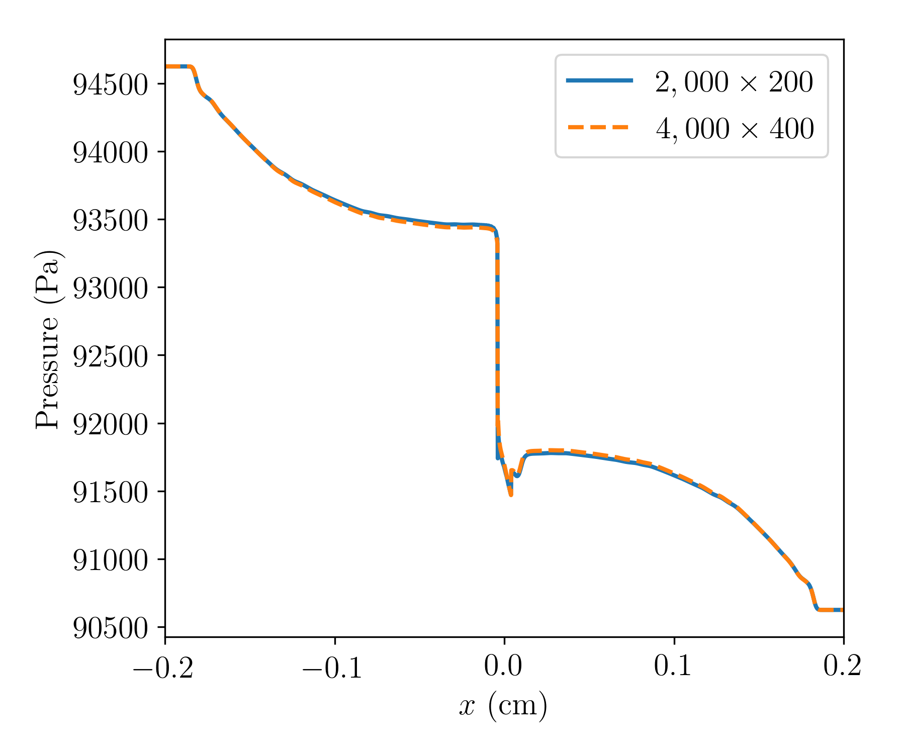
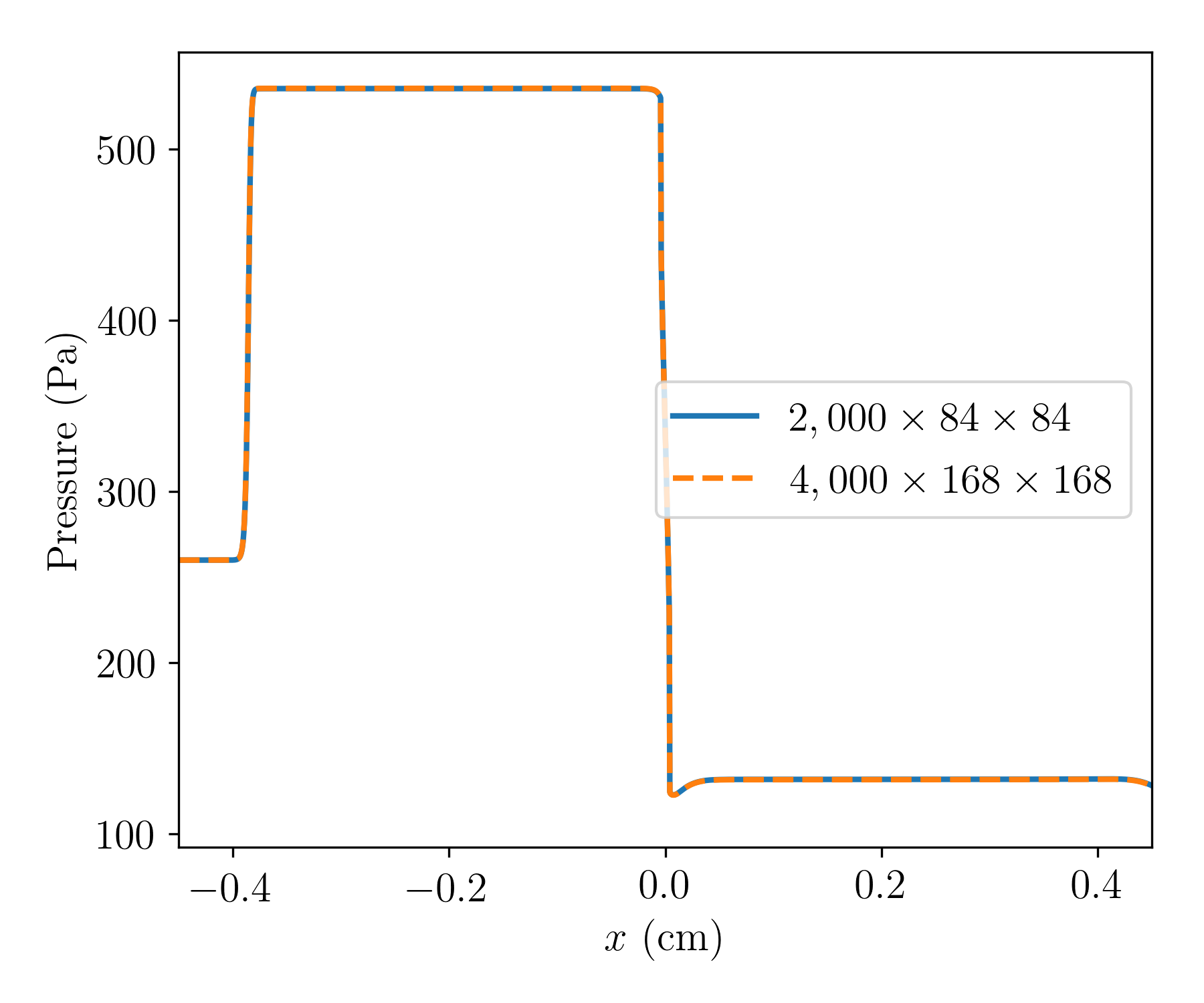
Figure 16: Convergence of a pore-resolved simulation: type “evaluation of a candidate equivalent pore”, $8\%\times 100\%$ pore geometry, initial pressure jump of $4,000\ \mathrm{Pa}$, and pressure profile in the central $x$-$y$ plane at $t=5.3\ \mathrm{\mu s}$ (left); and type “shock-porous-wall interaction”, $2/7\times 2/7$ pore geometry, $V_{s}=279.4\ \mathrm{m\ s^{-1}}$, and pressure profile in the central $x$-$y$ plane at $t=23.46\ \mathrm{\mu s}$ (right).

References

- Apte and Yang [2001] Sourabh Apte and Vigor Yang. Unsteady flow evolution in porous chamber with surface mass injection, part 1: Free oscillation. AIAA journal, 39(8):1577–1586, 2001. doi: https://doi.org/10.2514/2.1483.
- Avery et al. [2020] Philip Avery, Daniel Z Huang, Wanli He, Johanna Ehlers, Armen Derkevorkian, and Charbel Farhat. A computationally tractable framework for nonlinear dynamic multiscale modeling of membrane fabric. arXiv preprint arXiv:2007.05877, 2020.
- Beavers and Joseph [1967] Gordon S Beavers and Daniel D Joseph. Boundary conditions at a naturally permeable wall. Journal of Fluid Mechanics, 30(1):197–207, 1967. doi: https://doi.org/10.1017/S0022112067001375.
- Borker et al. [2019] Raunak Borker, Daniel Huang, Sebastian Grimberg, Charbel Farhat, Philip Avery, and Jason Rabinovitch. Mesh adaptation framework for embedded boundary methods for computational fluid dynamics and fluid-structure interaction. International Journal for Numerical Methods in Fluids, 2019. doi: https://doi.org/10.1002/fld.4728.
- Cruz et al. [2017] Juan R Cruz, Clara O’Farrell, Elsa Hennings, and Paul Runnells. Permeability of two parachute fabrics-measurements, modeling, and application. In 24th AIAA Aerodynamic Decelerator Systems Technology Conference, page 3725, 2017. doi: https://doi.org/10.2514/6.2017-3725.
- Ergun and Orning [1949] Sabri Ergun and Ao Ao Orning. Fluid flow through randomly packed columns and fluidized beds. Industrial & Engineering Chemistry, 41(6):1179–1184, 1949.
- Farhat et al. [1993] Charbel Farhat, Loula Fezoui, and Stéphane Lanteri. Two-dimensional viscous flow computations on the connecti on machine: Unstructured meshes, upwind schemes and massively parallel computations. Computer Methods in Applied Mechanics and Engineering, 102(1):61–88, 1993. doi: https://doi.org/10.1016/0045-7825(93)90141-J. URL http://www.sciencedirect.com/science/article/pii/004578259390141J.
- Farhat et al. [2003] Charbel Farhat, Philippe Geuzaine, and Gregory Brown. Application of a three-field nonlinear fluid–structure formulation to the prediction of the aeroelastic parameters of an f-16 fighter. Computers & Fluids, 32(1):3–29, 2003. doi: https://doi.org/10.1016/S0045-7930(01)00104-9.
- Gao et al. [2016] Zheng Gao, Richard D Charles, and Xiaolin Li. Numerical modeling of flow through porous fabric surface in parachute simulation. AIAA journal, 55(2):686–690, 2016. doi: https://doi.org/10.2514/1.J054997.
- Geuzaine et al. [2003] Philippe Geuzaine, Gregory Brown, Chuck Harris, and Charbel Farhat. Aeroelastic dynamic analysis of a full f-16 configuration for various flight conditions. AIAA journal, 41(3):363–371, 2003. doi: https://doi.org/10.2514/2.1975.
- Griffiths et al. [2013] IM Griffiths, PD Howell, and RJ Shipley. Control and optimization of solute transport in a thin porous tube. Physics of Fluids, 25(3):033101, 2013. doi: https://doi.org/10.1063/1.4795545.
- Huang et al. [2018a] Daniel Z Huang, Dante De Santis, and Charbel Farhat. A family of position-and orientation-independent embedded boundary methods for viscous flow and fluid–structure interaction problems. Journal of Computational Physics, 365:74–104, 2018a. doi: https://doi.org/10.1016/j.jcp.2018.03.028.
- Huang et al. [2020a] Daniel Z Huang, Philip Avery, and Charbel Farhat. An embedded boundary approach for resolving the contribution of cable subsystems to fully coupled fluid-structure interaction. International Journal for Numerical Methods in Engineering, 2020a. doi: https://doi.org/10.1002/nme.6322.
- Huang et al. [2020b] Daniel Z Huang, Philip Avery, Charbel Farhat, Jason Rabinovitch, Armen Derkevorkian, and Lee D Peterson. Modeling, simulation and validation of supersonic parachute inflation dynamics during mars landing. In AIAA Scitech 2020 Forum, page 0313, 2020b. doi: https://doi.org/10.2514/6.2020-0313.
- Huang et al. [2018b] Zhengyu Huang, Philip Avery, Charbel Farhat, Jason Rabinovitch, Armen Derkevorkian, and Lee D Peterson. Simulation of parachute inflation dynamics using an eulerian computational framework for fluid-structure interfaces evolving in high-speed turbulent flows. In 2018 AIAA Aerospace Sciences Meeting, page 1540, 2018b. doi: https://doi.org/10.2514/6.2018-1540.
- Judd et al. [1996] MJ Judd, MR Raupach, and JJ Finnigan. A wind tunnel study of turbulent flow around single and multiple windbreaks, part i: velocity fields. Boundary-Layer Meteorology, 80(1-2):127–165, 1996. doi: https://doi.org/10.1007/BF00119015.
- Karagiozis et al. [2011] K Karagiozis, R Kamakoti, F Cirak, and C Pantano. A computational study of supersonic disk-gap-band parachutes using large-eddy simulation coupled to a structural membrane. Journal of Fluids and Structures, 27(2):175–192, 2011. doi: https://doi.org/10.1016/j.jfluidstructs.2010.11.007.
- Kim and Peskin [2006] Yongsam Kim and Charles S Peskin. 2–D parachute simulation by the immersed boundary method. SIAM Journal on Scientific Computing, 28(6):2294–2312, 2006. doi: https://doi.org/10.1137/S1064827501389060.
- Lakshminarayan et al. [2014] V Lakshminarayan, C Farhat, and A Main. An embedded boundary framework for compressible turbulent flow and fluid–structure computations on structured and unstructured grids. International Journal for Numerical Methods in Fluids, 76(6):366–395, 2014. doi: https://doi.org/10.1002/fld.3937.
- Lin et al. [2010] John K Lin, Lauren S Shook, Joanne S Ware, and Joseph V Welch. Flexible material systems testing. NASA report CR-2010-216854, 2010.
- Ling et al. [2016] Bowen Ling, Alexandre M Tartakovsky, and Ilenia Battiato. Dispersion controlled by permeable surfaces: surface properties and scaling. Journal of Fluid Mechanics, 801:13–42, 2016.
- Main et al. [2017] Alex Main, Xianyi Zeng, Philip Avery, and Charbel Farhat. An enhanced FIVER method for multi-material flow problems with second-order convergence rate. Journal of Computational Physics, 329:141–172, 2017. doi: https://doi.org/10.1016/j.jcp.2016.10.028.
- Mendez and Nicoud [2008a] Simon Mendez and Franck Nicoud. Adiabatic homogeneous model for flow around a multiperforated plate. AIAA journal, 46(10):2623–2633, 2008a. doi: https://doi.org/10.2514/1.37008.
- Mendez and Nicoud [2008b] Simon Mendez and Franck Nicoud. Large-eddy simulation of a bi-periodic turbulent flow with effusion. Journal of Fluid Mechanics, 598:27–65, 2008b.
- Mendez et al. [2007] Simon Mendez, Franck Nicoud, and Thierry Poinsot. Large-eddy simulation of a turbulent flow around a multi-perforated plate. In Complex Effects in Large Eddy Simulations, pages 289–303. Springer, 2007.
- Muskat [1934] Morris Muskat. The flow of compressible fluids through porous media and some problems in heat conduction. Physics, 5(3):71–94, 1934. doi: https://doi.org/10.1063/1.1745233.
- Nassehi [1998] V Nassehi. Modelling of combined Navier–Stokes and Darcy flows in crossflow membrane filtration. Chemical Engineering Science, 53(6):1253–1265, 1998. doi: https://doi.org/10.1016/S0009-2509(97)00443-0.
- Panerai et al. [2017] Francesco Panerai, Arnaud Borner, Joseph C Ferguson, Nagi N Mansour, Eric C Stern, Harold S Barnard, Alastair A MacDowell, and Dilworth Y Parkinson. X-ray micro-tomography applied to nasa’s materials research: heat shields, parachutes and asteroids. NASA report ARC-E-DAA-TN39049, 2017.
- Patton et al. [1998] Edward G Patton, Roger H Shaw, Murray J Judd, and Michael R Raupach. Large-eddy simulation of windbreak flow. Boundary-Layer Meteorology, 87(2):275–307, 1998. doi: https://doi.org/10.1023/A:1000945626163.
- Roe [1981] Philip L Roe. Approximate Riemann solvers, parameter vectors, and difference schemes. Journal of Computational Physics, 43(2):357–372, 1981. doi: https://doi.org/10.1016/0021-9991(81)90128-5.
- Schmidt [2014] BE Schmidt. Compressible flow through porous media with application to injection. California Inst. of Technology IR-FM-2014.001, Pasadena, CA, 2014.
- Shepherd and Begeal [1988] JE Shepherd and DR Begeal. Transient compressible flow in porous materials. NASA STI/Recon Technical Report N, 88, 1988.
- Sutera and Skalak [1993] Salvatore P Sutera and Richard Skalak. The history of poiseuille’s law. Annual review of fluid mechanics, 25(1):1–20, 1993. doi: 10.1146/annurev.fl.25.010193.000245.
- Takizawa et al. [2012] Kenji Takizawa, Matthew Fritze, Darren Montes, Timothy Spielman, and Tayfun E Tezduyar. Fluid–structure interaction modeling of ringsail parachutes with disreefing and modified geometric porosity. Computational Mechanics, 50(6):835–854, 2012. doi: https://doi.org/10.1007/s00466-012-0761-3.
- Takizawa et al. [2017] Kenji Takizawa, Tayfun E Tezduyar, and Taro Kanai. Porosity models and computational methods for compressible-flow aerodynamics of parachutes with geometric porosity. Mathematical Models and Methods in Applied Sciences, 27(04):771–806, 2017. doi: https://doi.org/10.1142/S0218202517500166.
- Tutt et al. [2010] Benjamin Tutt, C Richard, S Roland, and Greg Noetscher. Development of parachute simulation techniques in ls-dyna. In 11th international LS-DYNA users conference, pages 25–36. Livermore Software Technology Corporation, 2010.
- Wang et al. [2001] Hao Wang, Eugene S Takle, and Jinmei Shen. Shelterbelts and windbreaks: mathematical modeling and computer simulations of turbulent flows. Annual Review of Fluid Mechanics, 33(1):549–586, 2001. doi: 10.1146/annurev.fluid.33.1.549.
- Wang et al. [2011] Kevin Wang, Arthur Rallu, J-F Gerbeau, and Charbel Farhat. Algorithms for interface treatment and load computation in embedded boundary methods for fluid and fluid–structure interaction problems. International Journal for Numerical Methods in Fluids, 67(9):1175–1206, 2011. doi: https://doi.org/10.1002/fld.2556.
- White [2006] Frank M White. Viscous fluid flow. McGraw-Hill New York, third edition, 2006.
- Wilson [1985] John D Wilson. Numerical studies of flow through a windbreak. Journal of Wind Engineering and Industrial Aerodynamics, 21(2):119–154, 1985. doi: https://doi.org/10.1016/0167-6105(85)90001-7.
- Wong [2019] Man Long Wong. High-order shock-capturing methods for study of shock-induced turbulent mixing with adaptive mesh refinement simulations. PhD thesis, Stanford University, 2019.
- Wong and Lele [2016] Man Long Wong and Sanjiva K Lele. Multiresolution feature detection in adaptive mesh refinement with high-order shock-and interface-capturing scheme. In 46th AIAA Fluid Dynamics Conference, page 3810, 2016. doi: https://doi.org/10.2514/6.2016-3810.
- Wong and Lele [2017] Man Long Wong and Sanjiva K Lele. High-order localized dissipation weighted compact nonlinear scheme for shock-and interface-capturing in compressible flows. Journal of Computational Physics, 339:179–209, 2017. doi: https://doi.org/10.1016/j.jcp.2017.03.008.