Barycentric interpolation on Riemannian and semi-Riemannian spaces

Abstract

Interpolation of data represented in curvilinear coordinates and possibly having some non-trivial, typically Riemannian or semi-Riemannian geometry is an ubiquitous task in all of physics. In this work we present a covariant generalization of the barycentric coordinates and the barycentric interpolation method for Riemannian and semi-Riemannian spaces of arbitrary dimension. We show that our new method preserves the linear accuracy property of barycentric interpolation in a coordinate-invariant sense. In addition, we show how the method can be used to interpolate constrained quantities so that the given constraint is automatically respected. We showcase the method with two astrophysics related examples situated in the curved Kerr spacetime. The first problem is interpolating a locally constant vector field, in which case curvature effects are expected to be maximally important. The second example is a General Relativistic Magnetohydrodynamics simulation of a turbulent accretion flow around a black hole, wherein high intrinsic variability is expected to be at least as important as curvature effects.

1 Introduction

Interpolation is necessary in a variety of physical problems, both in modeling and the analysis of measurements. When the data are distributed on a grid, the interpolation problem can be solved by the simplest of methods such as $n$-dimensional linear interpolation. However, when the data are scattered, more general methods are required, such as kriging or barycentric interpolation (Matheron, 1963; Floater et al., 2006).

In some cases the data can be both scattered and more importantly distributed on a manifold with some intrinsic geometry, such as for example the celestial sphere (Kamionkowski et al., 1997; The Polarbear Collaboration, 2014) or a planetary surface (Colony & Thorndike, 1984; Bindschadler & Scambos, 1991; Stohl et al., 1995). The data values may be also be constrained on some submanifold with an induced geometry. A typical example is the velocity field of matter, which in general or special relativity is constrained to have unit norm everywhere. These complications can also arise all at once, such as in simulations of strong gravity or of cosmological scales. In both cases, the base manifold is curved, and the velocity field is simultaneously constrained (Etienne et al., 2012; Adamek et al., 2014). Finally, in addition to having intrinsic geometry, the data might be known only as a distribution due to for example measurement uncertainties. This final complication requires statistical methods compatible with the data geometry (e.g. Pihajoki, 2017) and is beyond interpolation and the scope of this work.

When the data, now assumed precisely known, are bound by some geometry, the interpolation method used should respect this. The intuitive motivation is two-fold: Firstly, the interpolated value ought to be constructed using only the intrinsic variations within the data, so that the result is independent of the choice of coordinates. Secondly, the interpolated value should still be on the constraint manifold in order to avoid having to project the value back to the manifold.

A number of interpolation methods suited for scattered data on a specific Riemannian manifold, the two-dimensional sphere $S^{2}$, have been developed using a variety of approaches (e.g. Hardy & Göpfert, 1975; Wahba, 1981; Renka, 1984; Lawson, 1984; Pottmann & Eck, 1990; Alfeld et al., 1996; Cavoretto & Rossi, 2010). Comparatively few algorithms have been invented for interpolation on general Riemannian manifolds. However, a family of algorithms for generalized Hermite(–Birkhoff) interpolation on closed, compact Riemannian manifolds does exist (Narcowich, 1995; Dyn et al., 1999; Allasia et al., 2018), as well as a method for nearest neighbour interpolation of vector and tensor fields (Sharp et al., 2019). The authors know of no general purpose interpolation algorithms designed specifically for scattered data on semi-Riemannian manifolds.

In this paper we present an intrinsic, coordinate-independent generalization of the barycentric interpolation method to Riemannian and semi-Riemannian spaces. The method is suitable for interpolation of scattered tensorial data of any rank with or without constraints. In Section 2, we briefly review the concept of barycentric coordinates and the standard barycentric interpolation method. This is followed in Section 3 by our generalization. We show that the new method yields the linear precision characteristic of barycentric interpolation in a coordinate-independent manner, whereas the coordinate-only method fails to do so. We also provide approximate formulae with which our method can be put into a mathematically explicit form. In Section 4 we show numerical examples of the behaviour of our algorithm in the case of a curved Kerr spacetime. We provide here also the numerical implementation of the new method as a part of the Arcmancer ray-tracing library (Pihajoki et al., 2018).

2 Barycentric coordinates and interpolation

2.1 Barycentric coordinates

Barycentric interpolation is based on the notion of barycentric coordinates. Assume we have a convex polytope $P$ consisting of $N$ vertices $V_{1},\ldots,V_{N}$ in $n$ dimensions, with coordinates $\psi(V_{i})=\bm{\mathrm{x}}\in\mathbb{R}^{n}$ in the coordinate system $\psi$. The corresponding barycentric coordinate functions $\phi_{1},\ldots,\phi_{N}:\mathbb{R}^{n}\rightarrow\mathbb{R}$ are then defined by the conditions $\phi_{i}\geq 0$ and

$$\sum_{i=1}^{N}\phi_{i}(\bm{\mathrm{x}})\bm{\mathrm{x}}_{i}=\bm{\mathrm{x}}$$ (1)

$$\sum_{i=1}^{N}\phi_{i}=1,$$ (2)

where $\psi(X)=\bm{\mathrm{x}}\in\mathbb{R}^{n}$ are the coordinates of the point $X$ under consideration.

If $N=n+1$, the barycentric coordinates can be directly determined from equations (1) and (2). For $N>n+1$, the barycentric coordinate system is not unique. A review of barycentric coordinate systems and the methods to compute them is found in Floater (2015). Most of the coordinate systems were originally defined in two dimensions, but some, such as the maximum entropy (Sukumar, 2004), Wachspress (Wachspress, 1975) and mean value coordinate systems (Floater, 2003) generalize to higher dimensions. Of these, the Wachspress and mean value coordinates use global geometric properties such as areas, volumes or distances which make easy generalization to semi-Riemannian spaces difficult. On the other hand, the maximum entropy coordinates, briefly introduced in the following, can be readily generalized to semi-Riemannian spaces.

2.2 Maximum entropy coordinates

The key idea of maximum entropy coordinates is to consider the barycentric coordinates $\phi_{i}$ at a point $\bm{\mathrm{x}}$ as a discrete probability distribution. From this point of view, equation (1) is the statement $\langle\bm{\mathrm{x}}_{i}\rangle=\bm{\mathrm{x}}$, or that the mean of $\bm{\mathrm{x}}_{i}$ equals $\bm{\mathrm{x}}$ over the distribution $\{\phi_{i}\}$. Another way to formulate this is to note that equation (1) can be written as

$$\sum_{i=1}^{N}\phi_{i}(\bm{\mathrm{x}}_{i}-\bm{\mathrm{x}})=\sum_{i=1}^{N}\phi_{i}\Delta\bm{\mathrm{x}}_{i}=0,$$ (3)

where $\Delta\bm{\mathrm{x}}_{i}=\bm{\mathrm{x}}_{i}-\bm{\mathrm{x}}$. From this, we have correspondingly $\langle\Delta\bm{\mathrm{x}}_{i}\rangle=0$. The coordinates $\phi_{i}$ can then be found by maximizing the Shannon entropy $S(\{\phi_{i}\})=-\sum\phi_{i}\ln\phi_{i}$, subject to the constraints (2) and (3). This can be achieved by introducing the Lagrange multipliers $\alpha\in\mathbb{R}$ and $\bm{\mathrm{\beta}}\in\mathbb{R}^{n}$, and maximizing the function

$$\begin{split}&S({\phi_{i}},\alpha,\bm{\mathrm{\beta}})=\\ &\quad-\sum_{i=1}^{N}\phi_{i}\ln\phi_{i}+\alpha\left(\sum_{i=1}^{N}\phi_{i}-1\right)+\bm{\mathrm{\beta}}\cdot\sum_{i=1}^{N}\phi_{i}\Delta\bm{\mathrm{x}}_{i}.\end{split}$$ (4)

Setting the derivatives of equation (4) to zero yields the equations

$$Z=\sum_{i=1}^{N}Z_{i}=\exp(-\alpha+1)$$ (5)

$$Z_{i}=\exp(\bm{\mathrm{\beta}}\cdot\Delta\bm{\mathrm{x}}_{i})$$ (6)

$$\phi_{i}=\frac{Z_{i}}{Z}.$$ (7)

The constraint (3) then gives

$$\sum_{i=1}^{N}Z_{i}\Delta\bm{\mathrm{x}}_{i}=0,$$ (8)

from which $\bm{\mathrm{\beta}}$ and subsequently $\phi_{i}$ can be solved directly. Alternatively, the solution can be obtained from the equivalent minimization problem

$$\bm{\mathrm{\beta}}=\operatorname*{argmin}_{\bm{\mathrm{\beta}}^{\prime}}\ln Z(\bm{\mathrm{\beta}}^{\prime}),$$ (9)

which may be in some cases numerically easier (Sukumar, 2004; Hormann & Sukumar, 2008).

2.3 Barycentric interpolation

Barycentric coordinates have a natural application in interpolation. Assume we wish to interpolate some field $f(\bm{\mathrm{x}})$, where the codomain of $f$ could be any vector space over $\mathbb{R}$ in general, but for typical physical applications would be $\mathbb{R}$ itself or the space of vectors or tensors at a point. We know the values of $f$ at the vertices $\bm{\mathrm{x}}_{i}$, and wish to obtain the interpolant $\widehat{f}(\bm{\mathrm{x}})$ at $\bm{\mathrm{x}}$. When the barycentric coordinates $\phi_{i}$ of $\bm{\mathrm{x}}$ have been obtained, the barycentric interpolant is computed from

$$\widehat{f}(\bm{\mathrm{x}})=\sum_{i=1}^{N}\phi_{i}f(\bm{\mathrm{x}}_{i}).$$ (10)

The interpolation method (10) turns out to have linear precision, so that if $f(\bm{\mathrm{x}})$ is linear in the coordinates $\psi$, then $\widehat{f}=f$ inside the polytope $P$ (Floater et al., 2006).

3 Generalization to semi-Riemannian spaces

In the following, we now assume that the vertices $V_{i}$ are points on an $n$-dimensional Riemannian or semi-Riemannian manifold $M$ with a metric $g$ and some coordinate chart $\psi:M\rightarrow\mathbb{R}^{n}$. The data are taken to originate from an arbitrary rank $(r,s)$ tensor field $f\in\mathcal{T}^{r}_{s}(M)$, including scalar fields. Here $\mathcal{T}^{r}_{s}(M)$ is the space of all tensor fields on $M$, so that at each vertex $V_{i}$ sits a tensor $f(V_{i})\in T_{V_{i}}(M)^{r}_{s}$, where $T_{V_{i}}(M)^{r}_{s}$ is the space of all rank $(r,s)$ tensors at point $V_{i}$. We need a method to find the barycentric coordinates of $X$ with respect to the $V_{i}$. We also need to transform the data from the spaces $T_{V_{i}}(M)^{r}_{s}$ to the common space $T_{X}(M)^{r}_{s}$ to compute the interpolant.

3.1 Barycentric coordinates in curved spaces

In order to find a generalization of barycentric coordinates to semi-Riemannian spaces, we need to generalize the condition (3) to curved spaces. This amounts to finding a reasonable generalization for the difference of Cartesian position vectors $\Delta\bm{\mathrm{x}}_{i}$. An additional requirement for the object sought after is that it should be defined locally at the point $X\in M$, where we wish to compute the interpolant.

An object fulfilling these requirements is the tangent vector $\bm{\mathrm{z}}_{i}\in T_{X}(M)$ at $X$ of a geodesic $\gamma_{\bm{\mathrm{z}}_{i}}:\mathbb{R}\rightarrow M$ for which $\gamma_{\bm{\mathrm{z}}_{i}}(0)=X$ and $\gamma_{\bm{\mathrm{z}}_{i}}(1)=V_{i}$. Equivalently, the components of $\bm{\mathrm{z}}_{i}$ are the Riemann normal coordinates (RNC) of the point $V_{i}$ as developed around point $X$. The vectors $\bm{\mathrm{z}}_{i}$ are all defined at $X$, and are a coordinate independent concept, as is the sum $\sum_{i}\phi_{i}\bm{\mathrm{z}}_{i}$. Furthermore, for an Euclidean space with Cartesian coordinates, we get precisely $\bm{\mathrm{z}}_{i}=\Delta\bm{\mathrm{x}}_{i}$. While the RNC are often defined assuming an orthonormal basis of the tangent space $T_{X}M$ at $X$ (e.g. O’Neill, 1983; Lee, 1997), this is not strictly necessary and the components of $\bm{\mathrm{z}}_{i}$ can be computed in any local basis of $T_{X}M$ (Misner et al., 1973), such as the coordinate vector basis of the chart $\psi$. In the following, we use the coordinate vector basis of $\psi$ for all tensors.

Determining the vector $\bm{\mathrm{z}}_{i}$ for a given $X$ and each $V_{i}$ in general requires the solution of a boundary value problem

$$\begin{split}&\frac{\mathrm{d}^{2}\gamma_{\bm{\mathrm{z}}_{i}}(\lambda)^{a}}{\mathrm{d}\lambda^{2}}+\Gamma^{a}_{bc}\frac{\mathrm{d}\gamma_{\bm{\mathrm{z}}_{i}}(\lambda)^{b}}{\mathrm{d}\lambda}\frac{\mathrm{d}\gamma_{\bm{\mathrm{z}}_{i}}(\lambda)^{c}}{\mathrm{d}\lambda}=0\\ &\gamma_{\bm{\mathrm{z}}_{i}}(0)=X\quad\quad\gamma_{\bm{\mathrm{z}}_{i}}(1)=V_{i}.\end{split}$$ (11)

This can be done numerically by combining a numerical ordinary differential equation solver with a root-finding or optimization routine.

The new barycentric coordinate condition is now

$$\sum_{i=1}^{N}\phi_{i}\bm{\mathrm{z}}_{i}=0,$$ (12)

at the point $X$. The curved-space barycentric coordinates $\phi_{i}$ of $X$ can again be found by maximizing the entropy

$$\begin{split}&S(\{\phi_{i}\},\alpha,\bm{\mathrm{\beta}})=\\ &\quad-\sum_{i=1}^{N}\phi_{i}\ln\phi_{i}+\alpha\left(\sum_{i=1}^{N}\phi_{i}-1\right)+\sum_{i=1}^{N}\langle\bm{\mathrm{\beta}},\phi_{i}\bm{\mathrm{z}}_{i}\rangle,\end{split}$$ (13)

where again $\alpha\in\mathbb{R}$ but now $\bm{\mathrm{\beta}}\in T^{*}_{X}(M)$ is an element of the cotangent space at $X$, and the angle brackets denote the natural pairing of tangent and cotangent spaces so that $\left\langle\bm{\mathrm{\beta}},\bm{\mathrm{z}}_{i}\right\rangle=\beta_{a}z_{i}^{a}$ in the abstract index notation. The solution to the maximization problem is identical to equations (5)–(9), with $\Delta\bm{\mathrm{x}}_{i}$ everywhere replaced with $\bm{\mathrm{z}}_{i}$ and $\bm{\mathrm{\beta}}\cdot\Delta\bm{\mathrm{x}}_{i}$ by $\langle\bm{\mathrm{\beta}},\bm{\mathrm{z}}_{i}\rangle$.

It is interesting to note that to derive the barycentric coordinates for a curved space, only the connection is required, for computing the normal coordinates. A metric is not required, but for physically interesting cases, a metric typically exists, and then the natural choice for the connection is the metric (Levi–Civita) connection.

3.2 Interpolation of unconstrained data

For curved spaces, the interpolation formula (10) cannot be used directly. This is because the data $f(V_{i})$ are defined in different spaces with different base points $V_{i}$. To obtain the interpolant $\widehat{f}$ at $X$, these data must first be transported to $X$. For semi-Riemannian spaces, a natural solution is to parallel transport the data from each $V_{i}$ back to $X$, using the same geodesic $\gamma_{\bm{\mathrm{z}}_{i}}$ used to define the RNC of each $V_{i}$. This choice of curve is sufficient if we wish to retain the linear accuracy property of barycentric interpolation, as is seen below in Section 3.4.

In the case of scalar data, after parallel transport we have just equation (10) again. For rank $(r,s)$ tensorial data, $f(V_{i})=T(V_{i})^{a_{1}\cdots a_{r}}_{b_{1}\cdots b_{s}}$, we have to first solve the parallel transport problem

$$\begin{split}&\frac{\mathrm{d}T(\lambda)^{a_{1}\cdots a_{r}}_{b_{1}\cdots b_{s}}}{\mathrm{d}\lambda}=\biggl{(}-\Gamma^{a_{1}}_{cd}T(\lambda)^{c\cdots a_{r}}_{b_{1}\cdots b_{s}}-\ldots-\Gamma^{a_{r}}_{cd}T(\lambda)^{a_{1}\cdots c}_{b_{1}\cdots b_{s}}\\ &\quad+\Gamma^{c}_{b_{1}d}T(\lambda)^{a_{1}\cdots a_{r}}_{c\cdots b_{s}}+\ldots+\Gamma^{c}_{b_{s}d}T(\lambda)^{a_{1}\cdots a_{r}}_{b_{1}\cdots c}\biggr{)}v_{i}(\lambda)^{d}\end{split}$$ (14)

$$T(1)^{a_{1}\cdots a_{r}}_{b_{1}\cdots b_{s}}=T(V_{i})^{a_{1}\cdots a_{r}}_{b_{1}\cdots b_{s}},$$ (15)

where $v_{i}(\lambda)^{a}=\mathrm{d}\gamma_{\bm{\mathrm{z}}_{i}}(\lambda)^{a}/\mathrm{d}\lambda$, to obtain the parallel transported $\widetilde{T}^{a_{1}\cdots a_{r}}_{b_{1}\cdots b_{s}}=T(0)^{a_{1}\cdots a_{r}}_{b_{1}\cdots b_{s}}$. After the parallel transport, all quantities are now defined in the same space at the point $X$, and we can use equation (10) to obtain

$$\widehat{T}=\sum_{i=1}^{N}\phi_{i}\widetilde{T}_{i},$$ (16)

where the tensor indices have been suppressed.

3.3 Interpolation of constrained data

Often the field $f$ to be interpolated has additional constraints. The archetypal example in relativity is the four-velocity field $\bm{\mathrm{u}}$ of matter, which has to fulfill $g_{ab}u^{a}u^{b}=1$ everywhere. The existence of a constraint restricts the field $f(p)$ to a subspace $S_{p}\subset T_{p}(M)^{r}_{s}$ of the space of all rank $(r,s)$ tensors at each point $p\in M$. Here we assume that $S_{p}$ is a (semi-)Riemannian submanifold of $T_{p}(M)^{r}_{s}$ for each $p$, with a metric $g_{S}$, possibly induced from the metric $g$. If the constraint is compatible with parallel transport, we can still obtain the parallel transported data $\widetilde{T}_{i}$ at the interpolation point $X$. However, now the direct interpolant $\widehat{T}$ given by equation (16) is in general not a member of the constraint space $S_{p}$. For example in the case of unit vector fields, the magnitude of the interpolant is always less than or equal to unity in Riemannian spaces, and greater than or equal to unity for timelike unit vector fields in Lorentzian spaces. This is because the barycentric interpolant is a convex combination.

The problem can be solved by using the method to compute the barycentric coordinates in reverse. The constraint submanifold $S_{X}\subset T_{X}(M)^{r}_{s}$ has a geometry defined by the metric $g_{S}$ by assumption. We can find the interpolant $\widehat{T}$ by requiring that

$$\sum_{i=1}^{N}\phi_{i}\widetilde{t}_{i}=0,$$ (17)

where $\widetilde{t}_{i}$ are now the Riemann normal coordinates of the data $\widetilde{T}_{i}$ as developed at point $\widehat{T}$. In the case of no constraints, or $S_{p}=T_{p}(M)^{r}_{s}$, the geometry is flat since $T_{p}(M)^{r}_{s}$ is a vector space isomorphic to $\mathbb{R}^{r\times s}$, and we have $\widetilde{t}_{i}=\widehat{T}_{i}-\widehat{T}$. In this case, the equation (17) reduces to equation (16).

3.4 Proof of linear accuracy

In the following, we show that the interpolation method presented in this paper is the correct covariant generalization of barycentric interpolation in the sense that it preserves the property of linear accuracy in curved spaces in a coordinate-independent sense, whereas the usual coordinate space method fails to do so. Here we assume that the vertices $V_{i}$ where the data are located at are contained in a relatively small region compared to the curvature scale, as well as the scale of variation of the field from which the data are sampled. The accuracy of the curved space barycentric interpolation scheme described above can then be compared to the standard coordinate-only barycentric interpolation by using Taylor expansions up to second order.

Let the coordinates of the interpolation point $X$ be $\bm{\mathrm{x}}$ and the coordinates of the vertices $V_{i}$ be $\bm{\mathrm{x}}_{i}$, and let us write $\Delta\bm{\mathrm{x}}_{i}=\bm{\mathrm{x}}_{i}-\bm{\mathrm{x}}$. By expanding the geodesic $\gamma_{i}$ connecting $X$ and $V_{i}$ in a Taylor series, we find the following relations between the normal coordinates $\bm{\mathrm{z}}_{i}$ of the vertex $V_{i}$ and the coordinate differences $\Delta\bm{\mathrm{x}}_{i}$ (see also Brewin (2009))

$$z_{i}^{a} =\Delta x_{i}^{a}+\frac{1}{2}\Gamma^{a}_{bc}\Delta x_{i}^{b}\Delta x_{i}^{c}+O(\Delta\bm{\mathrm{x}}_{i}^{3})$$ (18)

$$\Delta x_{i}^{a} =z_{i}^{a}-\frac{1}{2}\Gamma^{a}_{bc}z_{i}^{b}z_{i}^{c}+O(\bm{\mathrm{z}}_{i}^{3}),$$ (19)

where the $O$-notation indicates that the quantities are given to second order in the components of $\Delta\bm{\mathrm{x}}_{i}$ and $\bm{\mathrm{z}}_{i}$, which are by assumption small. Here and throughout the rest of this section the Christoffel symbols and their derivatives are computed in the original coordinate basis $\psi$.

Let us then assume that the data to be interpolated is represented by a vector field $\bm{\mathrm{u}}\in\mathcal{T}^{1}_{0}(M)$. The following derivation works for general tensor fields as well, but the algebraic complexity grows significantly with each additional index. We evaluate $\bm{\mathrm{u}}$ at $V_{i}$ by propagating it from $X$ along the geodesic $\gamma_{i}$. The derivatives of $\bm{\mathrm{u}}$ with respect to the curve parameter $\lambda$ along $\gamma_{i}$ are then

$$\frac{\mathrm{d}u^{a}}{\mathrm{d}\lambda}(\lambda) =\Bigl{(}u^{a}_{;c}-\Gamma^{a}_{bc}u^{b}\Bigr{)}\frac{\mathrm{d}\gamma_{i}^{c}}{\mathrm{d}\lambda}$$ (20)

$$\begin{split}\frac{\mathrm{d}^{2}u^{a}}{\mathrm{d}{\lambda}^{2}}(\lambda)&=\Bigl{(}u^{a}_{;cd}-\Gamma^{a}_{bc}u^{b}_{;d}-\Gamma^{a}_{bd}u^{b}_{;c}-\Gamma^{a}_{bc,d}u^{b}\\ &\quad+\Gamma^{a}_{ce}\Gamma^{e}_{bd}u^{b}+\Gamma^{a}_{be}\Gamma^{e}_{cd}u^{b}\Bigr{)}\frac{\mathrm{d}\gamma_{i}^{c}}{\mathrm{d}\lambda}\frac{\mathrm{d}\gamma_{i}^{d}}{\mathrm{d}\lambda},\end{split}$$ (21)

where we have used the notation $u^{a}_{;cd}=\nabla_{d}\nabla_{c}u^{a}$ for covariant derivatives, which indicate the ‘true’ change in $\bm{\mathrm{u}}$ as opposed to purely coordinate or curvature related effects. Since $V_{i}=\gamma_{i}(1)$, we can express $\bm{\mathrm{u}}$ at $V_{i}$ to second order in $\bm{\mathrm{z}}_{i}$ through

$$\begin{split}u_{i}^{a}&=u_{0}^{a}+\frac{\mathrm{d}u^{a}}{\mathrm{d}\lambda}(0)+\frac{1}{2}\frac{\mathrm{d}^{2}u^{a}}{\mathrm{d}{\lambda}^{2}}(0)\\ &=u_{0}^{a}+(u^{a}_{;c}-\Gamma^{a}_{bc}u_{0}^{b})z_{i}^{c}\\ &\quad\quad+\frac{1}{2}\Bigl{(}u^{a}_{;cd}-2\Gamma^{a}_{bc}u^{b}_{;d}-\Gamma^{a}_{bc,d}u_{0}^{b}\\ &\quad\quad\quad+\Gamma^{a}_{ce}\Gamma^{e}_{bd}u_{0}^{b}+\Gamma^{a}_{be}\Gamma^{e}_{cd}u_{0}^{b}\Bigr{)}z_{i}^{c}z_{i}^{d}\end{split}$$ (22)

where we have used the symmetry of $z_{i}^{c}z_{i}^{d}$, and where now all Christoffel symbols and derivatives are evaluated at $X$.

When the data $\bm{\mathrm{u}}_{i}$ are parallel transported back to $X$ we get

$$\widetilde{u}_{i}^{a}=u_{0}^{a}+z_{i}^{c}u^{a}_{;c}+\frac{1}{2}z_{i}^{c}z_{i}^{d}u^{a}_{;cd}+O(z_{i}^{3}).$$ (23)

The curved space barycentric interpolant, equation (16), is then, to second order in $\bm{\mathrm{z}}_{i}$, given by

$$\widehat{u}^{a}=\sum_{i=1}^{N}\phi_{i}\widetilde{u}_{i}^{a}=u_{0}^{a}+\frac{1}{2}u^{a}_{;cd}\sum_{i=1}^{N}\phi_{i}z_{i}^{c}z_{i}^{d},$$ (24)

whereas the usual geometry-ignorant (‘flat’) barycentric interpolation yields similarly to second order

$$\begin{split}\widehat{u}^{a}&=\sum_{i=1}^{N}\chi_{i}u_{i}^{a}\\ &=u_{0}^{a}+\frac{1}{2}\left(u^{a}_{;cd}+C^{a}_{cd}(u)\right)\sum_{i=1}^{N}\chi_{i}\Delta x_{i}^{c}\Delta x_{i}^{d},\end{split}$$ (25)

where

$$C^{a}_{cd}(u)=\Gamma^{b}_{cd}u^{a}_{;b}-2\Gamma^{a}_{bc}u^{b}_{;d}+\Gamma^{a}_{ce}\Gamma^{e}_{bd}u_{0}^{b}-\Gamma^{a}_{bc,d}u_{0}^{b}$$ (26)

is the contribution from curvature, and we have used $\chi_{i}$ for the ‘flat’ barycentric coordinates. Here the curved space barycentric coordinates $\phi_{i}$ fulfill equation (12), whereas the ‘flat’ barycentric coordinates $\chi_{i}$ solve equation (3) instead.

Comparing equations (24) and (25), we can immediately point out our key results. First, when there is no curvature in the space or the coordinate system, so that $\Gamma^{a}_{bc}=\Gamma^{a}_{bc,d}=0$, both methods give equivalent results and are exact for locally linear fields, as expected. Furthermore, we see that if the vector field $\bm{\mathrm{u}}$ is locally linear, so that $u^{a}_{;cd}=0$, then the curved space method, equation (24) gives exact results, whereas the flat method, equation (25), does not. In fact, the flat method fails to give correct results even for locally constant fields, i.e. $u^{a}_{;cd}=u^{a}_{;c}=0$, due to the introduction of curvature effects. It should be emphasized here that the result in equation (24) requires both aspects of the new interpolation algorithm: computing the barycentric coordinates using the Riemann normal coordinates and the parallel transport of the data back to the interpolation point. As such, we conclude that the method presented here is a correct covariant generalization of the flat space barycentric interpolation method.

3.5 Approximate formulae

For generic problems, the interpolation method described in Section 3 cannot be put into an explicit form. Instead, several steps of numerical computation are required. Firstly, finding the Riemann normal coordinates of the vertices requires several solutions of a boundary value problem (11) for the geodesic equation. After this, the maximum entropy procedure to obtain the barycentric coordinates requires a solution to an optimization problem, equation (9), or a root finding problem, equation (12). Finally, if the data are constrained, a combined solution of finding Riemann normal coordinates and root finding, equation (17), is required. This can amount to a large computational cost per single interpolation. However, if the size of the region containing the vertices $V_{i}$ is comparatively small, and the curvature of the space is likewise small, explicit forms for the some sub-steps of the interpolation method can be derived in an approximate form.

The problem of finding Riemann normal coordinates can be transformed into an explicit form using series approximations (Brewin, 2009). For example, to second order, we have the formulae (18) and (19).

The minimization problem (9) can also be explicitly solved in the special case where the interpolation point $X$ is near the barycentre of the vertices $V_{i}$. In this case we have $\bm{\mathrm{\beta}}\sim 0$, and the barycentric coordinate condition (12) gives

$$\sum_{i=1}^{N}(1+\langle\bm{\mathrm{\beta}},\bm{\mathrm{z}}_{i}\rangle)\bm{\mathrm{z}}_{i}+O(\bm{\mathrm{\beta}}^{2})=0.$$ (27)

Discarding the higher order terms, this equation can be directly solved through

$$\bm{\mathrm{\beta}}=-(\mathsf{Z}^{T}\mathsf{Z})^{-1}\mathsf{Z}^{T}\bm{\mathrm{1}},$$ (28)

where

$$\mathsf{Z}^{T}=\begin{pmatrix}\bm{\mathrm{z}}_{1}&\cdots&\bm{\mathrm{z}}_{N}\end{pmatrix}\quad\text{($n\times N$ real matrix)}$$ (29)

$$\bm{\mathrm{1}}^{T}=(1,\ldots,1)\quad\text{($1\times N$ row vector)}.$$ (30)

This can be seen to be equivalent to the least squares solution of the equation $\mathsf{Z}\bm{\mathrm{\beta}}=-\bm{\mathrm{1}}$.

The parallel transport problem, equations (14)–(15) can also be solved approximately using series methods. If the RNC of a vertex $V$ are $\bm{\mathrm{z}}$, the data at $V$ is a rank $(r,s)$ tensor $T^{a_{1}\cdots a_{r}}_{b_{1}\cdots b_{s}}$ and $\Gamma^{a}_{bc}$ are the Christoffel symbols evaluated at the interpolation point $X$, then to first order the parallel transported tensor $\widetilde{T}$ at $X$ is

$$\begin{split}\widetilde{T}^{a_{1}\cdots a_{r}}_{b_{1}\cdots b_{s}}&=T^{a_{1}\cdots a_{r}}_{b_{1}\cdots b_{s}}+\Gamma^{a_{1}}_{cd}T^{c\cdots a_{r}}_{b_{1}\cdots b_{s}}z^{d}+\ldots+\Gamma^{a_{r}}_{cd}T^{a_{1}\cdots c}_{b_{1}\cdots b_{s}}z^{d}\\ &\quad-\Gamma^{c}_{b_{1}d}T^{a_{1}\cdots a_{r}}_{c\cdots b_{s}}z^{d}-\ldots-\Gamma^{c}_{b_{s}d}T^{a_{1}\cdots a_{r}}_{b_{1}\cdots c}z^{d}.\end{split}$$ (31)

And in particular for ubiquitous vectorial data, we have

$$\widetilde{T}^{a}=T^{a}+\Gamma^{a}_{bc}T^{b}z^{c}.$$ (32)

For interpolating constrained data, there is naturally no generic explicit solution. This is also true for such physically motivated simple cases as timelike unit vector fields on Lorentzian manifolds, but for these at least the solution can be condensed to a single implicit equation. Assume that we have previously derived the barycentric coordinates $\phi_{i}$ of the interpolation point $X$, and we have several timelike unit vectors $\bm{\mathrm{v}}_{i}$ that have been parallel transported from the vertices to $X$. We wish to find the interpolant $\bm{\mathrm{v}}$ fulfilling equation (17). We further assume that the metric at $X$ is in the Minkowski form, which can always be achieved by e.g. orthonormalizing the coordinate frame. In the space of timelike unit vectors at $X$, the Riemann normal coordinates of a vector $\bm{\mathrm{v}}_{i}$ with respect to the vector $\bm{\mathrm{v}}$ can now be found in the following manner. First, set

$$\bm{\mathrm{u}} =\bm{\mathrm{v}}_{i}-\bm{\mathrm{v}}-\left\langle\bm{\mathrm{v}}_{i}-\bm{\mathrm{v}},\bm{\mathrm{v}}\right\rangle$$ (33)

$$\bm{\mathrm{\widehat{u}}} =\frac{\bm{\mathrm{u}}}{\sqrt{-\left\langle\bm{\mathrm{u}},\bm{\mathrm{u}}\right\rangle}},$$ (34)

so that $\bm{\mathrm{\widehat{u}}}$ is the normalized part of $\bm{\mathrm{v}}_{i}-\bm{\mathrm{v}}$ orthogonal to $\bm{\mathrm{v}}$. Now

$$\bm{\mathrm{\gamma}}(\omega)=\cosh(\omega)\bm{\mathrm{v}}+\sinh(\omega)\bm{\mathrm{\widehat{u}}}$$ (35)

is a geodesic in the velocity space, with $\bm{\mathrm{\gamma}}(0)=\bm{\mathrm{v}}$ and $\bm{\mathrm{\gamma}}(\omega^{*})=\bm{\mathrm{v}}_{i}$, from which we get $\omega^{*}=\operatorname{arcosh}(\left\langle\bm{\mathrm{v}},\bm{\mathrm{v}}_{i}\right\rangle)$. Thus the Riemann normal coordinates $\bm{\mathrm{t}}_{i}$ of $\bm{\mathrm{v}}_{i}$ developed at point $\bm{\mathrm{v}}$ are

$$\bm{\mathrm{t}}_{i}=\operatorname{arcosh}(\left\langle\bm{\mathrm{v}},\bm{\mathrm{v}}_{i}\right\rangle)\bm{\mathrm{\widehat{u}}}.$$ (36)

The desired unit length interpolant $\bm{\mathrm{v}}$ is then found by solving $\sum_{i}\phi_{i}\bm{\mathrm{t}}_{i}=0$, a system of $n$ non-linear equations for the $n$ components of $\bm{\mathrm{v}}$.

3.6 When are curvature effects important?

Since the curved space computation is potentially more numerically demanding, it would be useful to know when exactly we can expect to benefit from such a procedure. The equation for the second order error of the flat barycentric interpolation, equation (25), provides an estimate for when curvature effects should be taken into account.

For scalar fields, we see that the only difference between flat and curved space barycentric interpolation is in the computation of the barycentric coordinates. This in turn depends on the difference between $\Delta\bm{\mathrm{x}}_{i}$, the coordinate differences between the vertex and the interpolation point, and $\bm{\mathrm{z}}_{i}$, the Riemann normal coordinates of the vertex with respect to the interpolation point. From equations (18) and (19) we see that this difference is proportional to the components of the connection and the amount of coordinate difference. Thus we can say that when the values of $\frac{1}{2}\Gamma^{a}_{bc}\Delta x_{i}^{b}\Delta x_{i}^{c}$ are small compared to $\Delta x_{i}^{a}$ itself, the curvature effects can be safely ignored for all scalar field interpolation.

For vector and tensor fields, the situation is more complicated. Firstly, we have the condition obtained above for scalar fields. In addition, from equation (25) we can deduce that curvature effects are likely to be important when the natural variability, represented by the second order covariant derivatives of the field, is of the same order as the curvature error contribution $C^{a}_{cd}(u)$.

In the following section, we will numerically investigate situations in curved spaces where the curvature effects are either crucial or of limited importance.

4 Numerical examples

4.1 Locally constant vector fields

To clearly illustrate the difference between the new method and coordinate space methods, we investigated numerically the interpolation error in a curved spacetime as a function of the size of the interpolation region. We computed the interpolation error in the squared norm and the components of a locally constant unit-norm vector field $\bm{\mathrm{u}}$ in the Kerr spacetime (Kerr, 1963), with a mass parameter $M=1$ and a dimensionless spin parameter $\chi=0.99$. Since the vector field was taken to be locally constant, we have $u^{a}_{;bc}=0$, and by the discussion in Section 3.6, the error caused by neglecting curvature should be significant.

The vector field was computed in the outgoing Cartesian Kerr–Schild coordinates $(t,x,y,z)$ (Kerr & Schild, 1965). Local constantness was achieved up to numerical precision by parallel transporting a vector $\bm{\mathrm{u}}_{0}=(g_{tt}^{-1/2},0,0,0)$ from the interpolation point to the data vertices using the Arcmancer code (Pihajoki et al., 2018). The vertices were defined to span the hypercube $[0,L]\times[10,10+L]\times[0,L]^{2}$, where $L$ determines the size of the interpolation region. The interpolation point was set in the coordinate center of the hypercube.

Figure 1: Interpolation error for a locally constant vector field as a function of the interpolation grid cell size $L$. The curved space barycentric method is indicated by filled circles, and the flat space barycentric method by crosses. Open squares indicate the analytic error estimate from equation (25). The black dashed line indicates the double precision floating point machine epsilon level. The figure includes two lines proportional to $L^{2}$ and $L^{3}$, drawn to guide the eye.

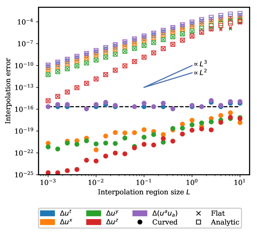
Figure 1 presents the absolute interpolation error of the curved space barycentric interpolation method, labelled ‘Curved’, and the coordinate space barycentric interpolation method, labelled ‘Flat’. We also computed the results of a standard $n$-linear coordinate interpolation method, which were identical to the flat space barycentric result to within numerical precision, as is expected when the data points lie on a regular grid (Sukumar, 2004). In addition, we computed the analytic error estimate for the flat barycentric method given by equation (25). The analytic estimate was found to be in excellent agreement with the numerical results up to interpolation region size of $\sim 1$, where higher order corrections can be expected to become significant. From the figure we see that the interpolation method presented here has essentially no error, with only round-off error from the numerical geodesic integration and optimization present. The level of numerical error seen in Figure 1 can be understood by considering the following rough estimate. If an exact process starting from some $x_{0}+\Delta$ and progressing to $x_{0}$ in $N$ small steps is approximated by an iterative numerical operation proceeding by consecutive differences, the resulting error is at most $\sim 2N\epsilon x_{0}+N\epsilon\Delta+O(\epsilon^{2})$, where $\epsilon$ is the machine epsilon, or the largest possible relative error when rounding to one (Goldberg, 1991). In this case, $\Delta$ is small and for the $u^{t}$ component $x_{0}\approx 1$, and for the $u^{x}$, $u^{y}$ and $u^{z}$ components $x_{0}=0$, which yields an estimate consistent with the errors seen in Figure 1, since we can expect $N$ to increase with $L$. In contrast to the curved space method, the standard coordinate-space methods are strictly bound by a non-zero error that scales at least quadratically with the size of the interpolation region. This result numerically illustrates the content of equations (24) and (25).

4.2 Interpolating a GRMHD simulation

We also investigated a situation, where the natural variability of the interpolated data can be expected to be high, and to possibly even surpass the effects of non-zero curvature. For this purpose, we chose a dataset consisting of a General Relativistic Magnetohydrodynamics (GRMHD) simulation of a turbulent, magnetized accretion flow around a Kerr black hole.

We used the harmpi code (Gammie et al., 2003; Noble et al., 2006) to run a three-dimensional simulation of a magnetized plasma torus around a Kerr black hole, with dimensionless spin of $\chi=0.5$. The initial conditions used were the standard initial conditions provided by the harmpi code, describing the Fishbone–Moncrief solution (Fishbone & Moncrief, 1976) of a poloidally magnetized plasma torus with a pressure maximum at a radius $r=12M$, where $M$ is the black hole mass. The number of (equidistant) grid points in the internal $(X_{1},X_{2},X_{3})$ coordinates was set to $(126,96,96)$. These coordinates correspond in a non-linear fashion to the spherical Kerr-Schild radial, polar and azimuthal coordinates $(r,\theta,\phi)$.

We evolved the simulation until $t=4250\,M$. From the final snapshot we created an output, downsampled by a factor of two by discarding data at every other grid point. Using the downsampled output, we interpolated the values of plasma density, internal energy, velocity and magnetic field at such points where the data had been discarded during downsampling, using both the method described in this paper and standard $n$-linear interpolation in the coordinate space. In the $n$-linear case, the velocity vectors were normalized to unit length after interpolation to obtain parity with the constrained barycentric method. All interpolation was done using the Cartesian ingoing Kerr-Schild coordinates (see e.g. Carter, 1968), in order not to introduce additional curvature from the use of a spherical coordinate chart.

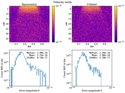
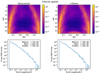
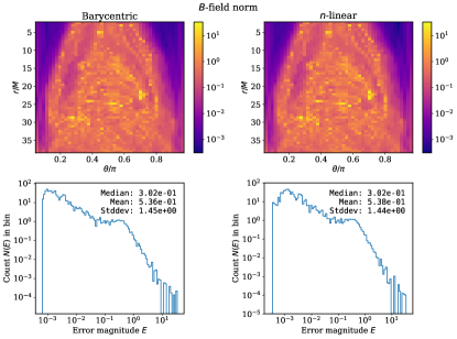
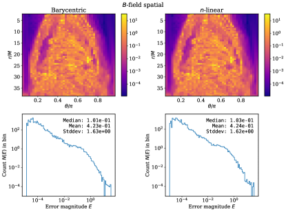
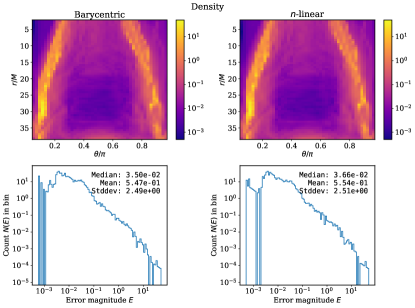
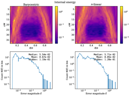
The interpolated values were then compared with the known values of the original snapshot, and the differences averaged over the azimuthal angle $\phi$, corresponding to averaging around the spin axis of the black hole. The results are shown in Figure 2. In the Figure, we plot the relative errors in the squared norm and spatial components of the fluid four-velocity $\bm{\mathrm{u}}$ and magnetic field $\bm{\mathrm{B}}$. The relative squared norm error for the velocity is computed as $(\left\|\hat{\bm{\mathrm{u}}}\right\|^{2}-\left\|\bm{\mathrm{u}}\right\|^{2})/\left\|\bm{\mathrm{u}}\right\|^{2}$, where $\hat{\bm{\mathrm{u}}}$ is the interpolated and $\bm{\mathrm{u}}$ the known reference value, and $\left\|\bm{\mathrm{u}}\right\|=\sqrt{\left|g_{ab}u^{a}u^{b}\right|}$. By relative spatial error we refer to $(\left\|\hat{\bm{\mathrm{u}}}_{s}-\bm{\mathrm{u}}_{s}\right\|^{2})/\left\|\bm{\mathrm{u}}_{s}\right\|^{2}$, where $\bm{\mathrm{u}}_{s}$ is vector $\bm{\mathrm{u}}$ with a zero time component. The errors for the magnetic field $\bm{\mathrm{B}}$ are computed similarly. For the scalars density and internal energy, Figure 2 shows the usual absolute relative difference with respect to the known values. In the Figure, we have also plotted histograms, and indicated the median, mean and standard deviations of all the relative errors.

Figure 2: Absolute relative errors in the squared norms and spatial components of the velocity and magnetic field ($B$-field), as well as density and internal energy, from left to right and top to bottom. All errors have been averaged over the azimuthal angle $\phi$. Each quantity has a $4\times 4$ panel where the top panels show a heatmap of the distribution of the error in the $(r,\theta)$ plane and bottom panels display histograms of the distribution of the relative error magnitudes. The leftmost two panels give the results corresponding to the barycentric method presented in this paper, and the rightmost two panels give the results of a standard $n$-linear coordinate interpolation method, combined with a normalization of the resulting velocity vector.

In Figure 3, we have plotted separately from equation (25) the ratio $\xi$ between the squared norm of the interpolation error due to the curvature terms and the error due to intrinsic variability, as represented by the covariant second derivative. For velocity, we computed

$$\xi(u)=\frac{\left\|\frac{1}{2}C^{a}_{bc}(u)\sum_{i}\chi_{i}\Delta x^{b}_{i}\Delta x^{c}_{i}\right\|^{2}}{\left\|\hat{u}^{a}-u_{0}^{a}-\frac{1}{2}C^{a}_{bc}(u)\sum_{i}\chi_{i}\Delta x^{b}_{i}\Delta x^{c}_{i}\right\|^{2}},$$ (37)

where the denominator is equivalent to $u^{a}_{;bc}\sum_{i}\chi_{i}\Delta x^{b}_{i}\Delta x^{c}_{i}$. The ratio $\xi(B)$ for magnetic field was computed similarly. As in Figure 2, the errors have been averaged over the azimuthal angle $\phi$.

Figure 3: Top panel: Heatmaps (top) and distributions (bottom) of the ratio of the curvature error to the intrinsic variability error, equation (37). The leftmost two panels show the result for the magnetic field and the rightmost two panels show the result for the velocity field. Bottom panel: The median ratio of the curvature error to the intrinsic variability error as a function of the radial distance $r$ from the black hole. Shaded area indicates the limits of one Median Absolute Deviation. A black line segment proportional to $r^{-2}$ has been added to help guide the eye.

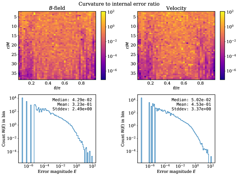
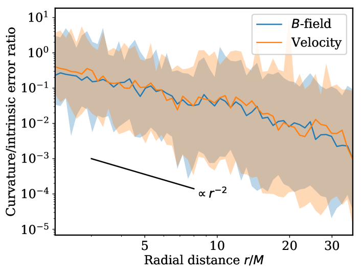
From Figure 3, we see that for at least this particular GRMHD simulation, the strong internal variability of the velocity field and the magnetic field dwarfs the curvature effects on the interpolation error. When the bulk of the simulation volume is considered as a whole, the median curvature contribution to the error is only on the order of $\sim 5\%$ of the error caused by the strong intrinsic variability. This is not unexpected, since the magnetized torus rotating around the black hole is subject to the magneto-rotational instability (MRI) (Balbus & Hawley, 1991), and will develop strong turbulence and corresponding intrinsic variability. However, even in this case of strong intrinsic variability, we can see from Figure 3 that when regions closer to the black hole are considered, the curvature errors can surpass intrinsic variability errors. This is potentially important, since in the light of the recent Event Horizon Telescope (EHT) results (Event Horizon Telescope Collaboration, 2019a), it is precisely these regions near the black hole event horizon that are expected to be most interesting. This is due to the fact that in the EHT data, the observable ring-like feature, which is used to constrain the black hole mass and spin, and attempt to separate General Relativity from other gravitational theories, is found in the immediate vicinity of the black hole event horizon, at $\sim 11~{}M$ (Event Horizon Telescope Collaboration, 2019b). From Figure 3, we see that the curvature error at this distance might be expected to be around $10\%$ of the intrinsic magnetic or velocity field error, albeit with a large scatter. This indicates that when interpolating future observational data at these distances, accounting for the spacetime curvature can potentially be important.

The results in Figure 3 might conceivably have some dependence on the resolution of the GRMHD simulation. However, from equation (25) we see that the possible resolution dependence of the curvature to intrinsic error ratio can only emerge from the ratios between vector field component magnitudes, and their first and second covariant derivatives. In a simulation such as the one used in this work, the simulation grid can be assumed to represent an implicit block filter, which is convolved with the ’true’ field to yield an effective large eddy simulation (e.g. Miesch et al., 2015). In this case, if the true smallest variability scales are much smaller than the grid size, the ratios of the maximum values of the vector field components and their derivatives should be independent of the grid resolution. Correspondingly the ratio between the maximum intrinsic and curvature errors should be resolution independent as well, as long as these assumptions hold. However, it should be noted that an increase in the resolution of the simulation will naturally always decrease the total absolute interpolation error.

Finally, as can be expected from the results in Figure 3, the interpolation errors for both vector quantities, velocity and magnetic field, shown in Figure 2, are quite similar for both methods. For the scalar quantities, density and internal energy, the results are likewise nearly identical. On the whole, the curved-space barycentric method gives more accurate results in the case of high intrinsic variability as well, but the improvement in the median error is only on the order of percents. This is a much more modest improvement when compared to the locally constant field in Section 4.1.

5 Conclusions

We have presented a covariant generalization of the barycentric interpolation method, suitable for constrained or unconstrained data on Riemannian and semi-Riemannian manifolds. The method is based on computing barycentric coordinates of an interpolation point using Riemann normal coordinates and parallel transport of all data to the interpolation point before computing the interpolant. The same approach also allows interpolation of constrained data without violating the constraint.

We have shown that the new method attains the linear precision property of barycentric interpolation in a coordinate-invariant sense, whereas the coordinate-only method is unable to replicate accurately even locally constant vector or tensor fields. This property was demonstrated in practice by interpolating data sampled from a locally constant vector field defined in a Kerr spacetime. The results showed that for interpolation regions ranging over four orders of magnitude in edge length $L$, the method presented here gave exact results up to floating point precision, whereas the coordinate-only method had an error proportional to at least $L^{2}$.

We further investigated the performance of the new method in the context of a General Relativistic Magnetohydrodynamics simulation, where the interpolated fields are highly non-linear. Here we saw that even though the intrinsic variability of the data was high, the barycentric method still provided improvements on the order of a few percent level.

This paper opens up some interesting new avenues for future work. An obvious followup is to investigate numerically efficient implementations of the new method and to compare the accuracy and computational cost to existing interpolation methods in a larger numerical survey. In addition, for certain geometries and choices of coordinates and/or vertex positions, the formulae may admit solutions in explicit form. This would provide an immediate computational speedup for that particular problem. Finally, there is the suggestion that similar straightforward covariant generalizations might be found for other known interpolation methods as well. Such generalizations might prove particularly useful for GRMHD simulation codes. This is because typically finite-volume simulations use high-order interpolation schemes to reconstruct grid cell boundary values from cell averaged values. High-order methods that take coordinate curvature into account do exist (Mignone, 2014) and are used in GRMHD simulations (e.g. White et al., 2016). However, the results in this paper suggest that in strong gravity situations, the spacetime curvature also needs to be accounted for.

References

- Adamek et al. (2014) Adamek J., Durrer R., Kunz M., 2014, Classical Quant. Grav., 31, 234006
- Alfeld et al. (1996) Alfeld P., Neamtu M., Schumaker L. L., 1996, J. Comput. Appl. Math., 73, 5
- Allasia et al. (2018) Allasia G., Cavoretto R., Rossi A. D., 2018, Appl. Math. Comput., 318, 35
- Balbus & Hawley (1991) Balbus S. A., Hawley J. F., 1991, ApJ, 376, 214
- Bindschadler & Scambos (1991) Bindschadler R. A., Scambos T. A., 1991, Science, 252, 242
- Brewin (2009) Brewin L., 2009, Classical Quant. Grav., 26, 175017
- Carter (1968) Carter B., 1968, Phys. Rev., 174, 1559
- Cavoretto & Rossi (2010) Cavoretto R., Rossi A. D., 2010, J. Comput. Appl. Math., 234, 1505
- Colony & Thorndike (1984) Colony R., Thorndike A. S., 1984, J. Geophys. Res. Oceans, 89, 10623
- Dyn et al. (1999) Dyn N., Narcowich F. J., Ward J. D., 1999, Constr. Approx., 15, 175
- Etienne et al. (2012) Etienne Z. B., Paschalidis V., Liu Y. T., Shapiro S. L., 2012, Phys. Rev. D, 85, 024013
- Event Horizon Telescope Collaboration (2019a) Event Horizon Telescope Collaboration 2019a, ApJ, 875, L1
- Event Horizon Telescope Collaboration (2019b) Event Horizon Telescope Collaboration 2019b, ApJ, 875, L6
- Fishbone & Moncrief (1976) Fishbone L. G., Moncrief V., 1976, ApJ, 207, 962
- Floater (2003) Floater M. S., 2003, Comput. Aided Geom. Des., 20, 19
- Floater (2015) Floater M. S., 2015, Acta Numer., 24, 161–214
- Floater et al. (2006) Floater M. S., Hormann K., Kós G., 2006, Adv. Comput. Math., 24, 311
- Gammie et al. (2003) Gammie C. F., McKinney J. C., Tóth G., 2003, ApJ, 589, 444
- Goldberg (1991) Goldberg D., 1991, ACM Comput. Surv., 23, 5
- Hardy & Göpfert (1975) Hardy R. L., Göpfert W. M., 1975, Geophys. Res. Lett., 2, 423
- Hormann & Sukumar (2008) Hormann K., Sukumar N., 2008, Comput. Graph. Forum, 27, 1513
- Kamionkowski et al. (1997) Kamionkowski M., Kosowsky A., Stebbins A., 1997, Phys. Rev. D, 55, 7368
- Kerr (1963) Kerr R. P., 1963, Phys. Rev. Lett., 11, 237
- Kerr & Schild (1965) Kerr R. P., Schild A., 1965, in Proc. Symp. Appl. Math. p. 199
- Lawson (1984) Lawson C. L., 1984, Rocky Mountain J. Math., 14, 177
- Lee (1997) Lee J. M., 1997, Riemannian manifolds: an introduction to curvature. Graduate Texts in Mathematics, Springer-Verlag New York, Inc., New York, NY 10010, USA
- Matheron (1963) Matheron G., 1963, Econ. Geol., 58, 1246
- Miesch et al. (2015) Miesch M., et al., 2015, Space Sci. Rev., 194, 97
- Mignone (2014) Mignone A., 2014, J. Comput. Phys., 270, 784
- Misner et al. (1973) Misner C. W., Thorne K. S., Wheeler J. A., 1973, Gravitation. W.H. Freeman and Company, New York, NY 10010, USA
- Narcowich (1995) Narcowich F., 1995, J. Math. Anal. Appl., 190, 165
- Noble et al. (2006) Noble S. C., Gammie C. F., McKinney J. C., Del Zanna L., 2006, ApJ, 641, 626
- O’Neill (1983) O’Neill B., 1983, Semi-Riemannian Geometry. Pure and Applied Mathematics, Academic Press, San Diego, CA 21101-4495, USA
- Pihajoki (2017) Pihajoki P., 2017, MNRAS, 472, 3407
- Pihajoki et al. (2018) Pihajoki P., Mannerkoski M., Nättilä J., Johansson P. H., 2018, ApJ, 863, 8
- Pottmann & Eck (1990) Pottmann H., Eck M., 1990, Comput. Aided Geom. Des., 7, 313
- Renka (1984) Renka R. J., 1984, ACM Trans. Math. Softw., 10, 417
- Sharp et al. (2019) Sharp N., Soliman Y., Crane K., 2019, ACM Trans. Graph., 38
- Stohl et al. (1995) Stohl A., Wotawa G., Seibert P., Kromp-Kolb H., 1995, J. Appl. Meteorol., 34, 2149
- Sukumar (2004) Sukumar N., 2004, Int. J. Numer. Methods Eng., 61, 2159
- The Polarbear Collaboration (2014) The Polarbear Collaboration 2014, ApJ, 794, 171
- Wachspress (1975) Wachspress E. L., 1975, A rational finite element basis. Mathematics in Science and Engineering, Elsevier, Burlington, MA
- Wahba (1981) Wahba G., 1981, SIAM J. Sci. Comput., 2, 5
- White et al. (2016) White C. J., Stone J. M., Gammie C. F., 2016, ApJS, 225, 22