Hall conductivity of a Sierpinski carpet

Abstract

We calculate the Hall conductivity of a Sierpinski carpet using Kubo-Bastin formula. The quantization of Hall conductivity disappears when we increase the depth of the fractal. The Hall conductivity is no more proportional to the Chern number. Nevertheless, these quantities behave in a similar way showing some reminiscence of a topological nature of the Hall conductivity. We also study numerically the bulk-edge correspondence and find that the edge states become less manifested when the depth of Sierpinski carpet is increased.

I Introduction

Fractals were very popular in 1980th and various properties of fractals were intensively studied at that time HavAbr1987 ; Tosatti_1986 ; Feder_1988 . Most of these works were focused on classical fractal systems; at the same time, it turned out that quantum properties of fractals are also unusual and interesting. For example, fractals have Cantor-like energy spectrum, which makes them similar to quasicrystals Domany_1983 . At that time, studies of quantum properties of fractal structures were of purely theoretical interest. With recent technological advances, fractals can be produced by both nanofabrication methods and manipulation of individual molecules on metal surfaces Polini_etal2013 ; Gibertini_etal2009 ; Shang_etal2015 ; Kempkes_etal2018 . This enhances the interest in a deeper understanding of the field. Recent theoretical works concerning quantum effects in fractals consider transport properties Veen2016 ; Veen2017 ; SongZhangLi2014 , plasmons Westerhout2018 , Anderson localization SticAkh2016 ; KosKrzys2017 , topological properties Brzezetal2018 ; AgPaiShen2018 ; Pal_etal2019 ; PaiPrem2019 , and other related topics Golmankhaneh2019 ; Akal2018 ; PalSaha2018 ; NandChak2016 ; NandPal2015 . The conductivity of fractals is especially interesting, due to possible experimental applications, and definitely deserves more attention.

In a seminal work TKNN1982 Thouless et al. established that the off-diagonal (Hall) conductivity of two-dimensional electron gas in magnetic field is proportional to the topological invariant called Chern number and is, therefore, closely related to topological properties of the system. The derivation rely on translational invariance of the system, thus the theory cannot be directly applied to quasiperiodic or fractal structures lacking the translational invariance. For quasiperiodic systems, one can obtain non-trivial topological properties of Hall conductivity by looking at the Brillouin zone as a non-commutative manifold KrausZilbl2015 ; Tran_etal2015 ; Bellissard1992 . The same is true for disordered systems Bellisard1994 ; Prodan2011 . To our knowledge, the relation between Hall conductivity and Chern numbers is still an open question for the case of fractals. A clarification of this issue could also provide better understanding of fracton topological order, another hot subject in contemporary condensed matter physics Halasz_etal2017 ; Devakul_etal_2019 .

It is also known for the systems with integer dimensions that quantization of Hall conductivity is closely related to the existence of edge states, in the form of the so called bulk-edge correspondense Halperin1982 ; Hatsugai1993 ; MongShiv2011 . The terms edge and bulk can be well defined for the systems without holes, or, at least, for a system, which has an integer dimension and finite number of holes. A fractal has an infinite number of holes, and the distribution of these holes is dense. Therefore the difference between edge states and bulk states should be carefully checked. This can be useful for better understanding of the Hall conductivity of fractals. One way to do this is to study various approximations to fractals with the holes of different scales.

Chern numbers for a Sierpinski carpet were calculated recently in Ref. Brzezetal2018, . The authors have concluded that the Chern numbers of a fractal are still quantized in some energy regions; in this sense, fractals still can possess non-trivial topological properties. Ref. Brzezetal2018, also studied Hall conductivity by calculating the variance of level spacings and its response to an added disorder. Technically, it was done by application of random matrix theory. However, the applicability of this approach to Sierpinski fractals is questionable, since the latter, strictly speaking, are not disordered systems. It was shown that the level-spacing distribution for some kind of fractals and quasiperiodic systems can have power-law behavior which cannot be described within the framework of the conventional random matrix theory IlKatSheng2019 ; MachFuj1986 ; Hernando2015 . Even if one can apply the latter to the spectrum of Sierpinski carpet, it is not enough to make definite conclusions on the quantization of Hall conductivity. Hence, the variance of level spacing distribution is not the most reliable tool to determine localization properties and their connection to the Hall conductivity.

In this work we examine relations between Hall conductivity and topological properties of Sierpinski carpet. In order to do this, we calculate the Hall conductivity and quasi-eigenstates for various iterations of Sierpinski carpet and investigate how they behave when the fractal depth is increased. We also compare our results with the calculated Chern numbers from the article Brzezetal2018 .

II The model

To study fractal structures, we use the single-orbital tight-binding Hamiltonian in the nearest-neighbor approximation, that is, the same model as in Refs. Veen2016, ; Veen2017, :

$$H=-t\sum_{\langle ij\rangle}e^{i\phi_{ij}}c^{\dagger}_{i}c_{j}\,,$$ (1)

where $c^{\dagger}_{i}$ creates fermion on a lattice site $i$, and $\langle ij\rangle$ denotes the nearest-neighbor sites belonging to the studied fractal. The influence of magnetic field is modeled by the standard Peierls substitution: $\phi_{ij}=2\pi/\Phi_{0}\int^{j}_{i}\mathbf{A}\,\mathbf{dr}$, where $\mathbf{A}$ is the vector potential and $\Phi_{0}=hc/e$ is the flux quantum. We use Landau gauge $\mathbf{A}=(-By,0,0)$.

We start with a square lattice of the size $3^{D_{f}}\times 3^{D_{f}}$. Then, we iteratively add holes, which gives us the realizations of Sierpinski carpet with varying depths. At first, we add the central hole of size $3^{D_{f}-1}\times 3^{D_{f}-1}$, then we add holes with size $3^{D_{f}-2}\times 3^{D_{f}-2}$, and so on. We can stop at any number of iterations $I_{f}$ less than $D_{f}$. The maximum depth of fractal on a given lattice is $D_{f}$. If $I_{f}=D_{f}$, the size of a hole is equal to one site. Examples of different iterations are given in Fig. 1

These structures have two parameters $I_{f}$ and $D_{f}$ that describe various approximations of Sierpinski carpet. They also describe a transition from the usual square lattice with dimension 2, to Sierpinski carpet with fractional dimension equal to $\ln 8/\ln 3$.

In order to calculate the density of states and Hall conductivity we use the real-space approaches described in Refs. Hams2000, ; Shengjun2010, ; Garcila_etal2015, ; ShengjunEdo2016, . Using these methods, we are able to calculate electronic properties for 6 iterations of Sierpinski carpet without any diagonalization.

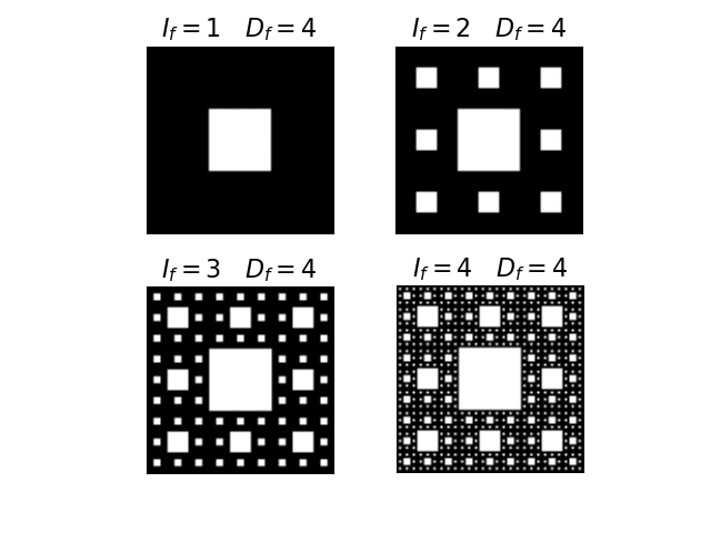
Figure 1: The examples of studied fractal structures. The size of the large square is $3^{D_{f}}\times 3^{D_{f}}$ sites with $D_{f}=4$ and different number of iterations $I_{f}$. With every iterations, new holes are deleted. The size of smallest holes is $3^{D_{f}-I_{f}}\times 3^{D_{f}-I_{f}}$.

III Results

III.1 Density of states

Let us at first shortly describe the numerical method which we use. We calculate density of states (DoS) for different fractal depths and iterations using a method based on the time evolution operator Hams2000 ; Shengjun2010 . We start the evolution of a quantum system with a random initial state $|\psi\rangle$, which is normalized so that $|\psi|^{2}=1$. The density of states is calculated via Fourier transform of the correlation function by averaging over initial random samplings Hams2000 ; Shengjun2010 :

$$d(\epsilon)=\langle\psi|\delta(\epsilon-H)|\psi\rangle=$$

$$=\frac{1}{2\pi}\int^{+\infty}_{-\infty}e^{i\epsilon\tau}\langle\psi|e^{-i\tau H}|\psi\rangle d\tau$$

Since density of states is a self-averaged quantity, it does not depend on the choice of the state $|\psi\rangle$ for large enough systems.

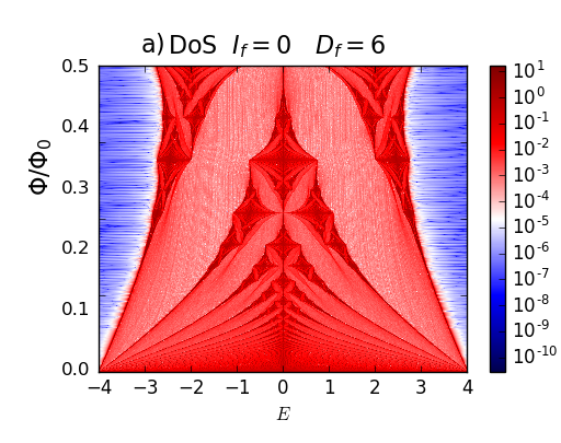
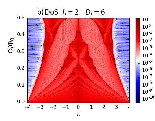
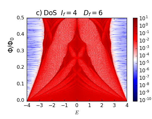
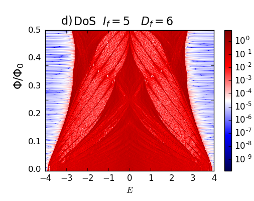
Figure 2: Pictures of DoS depending on magnetic field – Hofstadter butterflies (magnetic field $B$ corresponds to variations of $\Phi/\Phi_{0}$ from $0$ to $0.5$) for different iterations of Sierpinski carpet in a square of size $3^{D_{f}}\times 3^{D_{f}}$ and $D_{f}=6$: a) shows $I_{f}=0$ iteration, b) shows $I_{f}=2$ iterations, c) shows $I_{f}=4$ iterations, d) shows $I_{f}=5$ iterations. The differences between a), b) and c) are small. New peaks and gaps appear in the picture d).

In Fig. 2, we show the calculated density of states for various magnetic fields corresponding to $\Phi/\Phi_{0}$ changing from $0$ to $0.5$, $\Phi$ is the magnetic flux through the smallest element for a given structure. The energy $E$ is measured in values of hopping $t$ of the Hamiltonian (1). These pictures of Hofstadter butterflies Hofstadter1976 are calculated for $D_{f}=6$ and $I_{f}=0,2,4,5$.The figure demonstrates fractal structure of states and gaps due to additional period in hoppings associated with magnetic flux.

From these pictures one can see that for $I_{f}=0,2,4$ DoS is basically the same for all magnetic fields. The structure of Hofstadter butterfly with $I_{f}=5$ is different from the previous cases. Many more states appear and small gaps open for some magnetic fields (new red lines and white dots in Fig. 2 (d)). Therefore, $I_{f}=5$ seems to be the minimal depth that is needed to catch the peculiarities of quantum states in this particular fractal.

In Fig. 3, DoS is displayed for fractals with $I_{f}=5$, $D_{f}=6$ and $I_{f}=D_{f}=6$, $\Phi/\Phi_{0}=0.25$. The change from $I_{f}=5$ to $I_{f}=6$ is clear: a gap opens in the middle of the spectrum, and there are more states between peaks (around energy $E=2$). Density of states for $I_{f}=5$ is flatter in that region.

We also calculated DoS for $I_{f}=D_{f}=4$ and $I_{f}=D_{f}=5$. The results are visually almost indistinguishable from $I_{f}=D_{f}=6$. Hence, DoS converges for samples with maximum number of iterations and approaches the thermodynamic limit of a full fractal. For cases with $I_{f}<D_{f}<6$ we also observe that DoS changes only a little while a transition to another regime occurs when going from $I_{f}<D_{f}-1$ to $I_{f}=D_{f}-1$. Due to this transition, one cannot properly approximate the full fractal, if the smallest holes are absent in the sample.

The occurrence of the transition can be explained by the following reasoning. Before transition point the sample can still be treated as a bulk and the effective dimension is an integer. The holes in the sample can be seen as some additional disorder. When $I_{f}$ becomes equal to $5$ the distance between holes becomes comparable to the size of a site. Only at this point, the effective dimension of a sample becomes non-integer. The difference between cases $I_{f}=5$ and $I_{f}=6$ also can be explained by the difference in their non-integer dimensions. Proper approximation to Sierpinski carpet is only achieved when $I_{f}=D_{f}$.

Let us consider a square with one hole $I_{f}=1$ and then increase the number of sites $D_{f}$. This is an approximation of a two dimensional system. The cases of $D_{f}=1$ and $D_{f}=2$ correspond to the Sierpinski carpets with $D_{f}=I_{f}$ and $D_{f}=I_{f}-1$, since the average distances between holes are 1 site and 3 sites. These systems do not behave as two dimensional systems: $D_{f}=I_{f}=1$ is just a one dimensional cycle. However, in the case of $I_{f}=1$, for $D_{f}=3$, the sample already has DoS similar to a two dimensional sample. Therefore, we assume that samples with $I_{f}<D_{f}-1$ approximate systems with integer dimensions and transition of physical parameters should happen, when $I_{f}=D_{f}-1$.

We can think about this effect as a crucial property of exact scaling symmetry of fractals. Even the smallest breakage of scaling symmetry leads to effective integer dimension rather than fractional. Every site is an edge site in a sample with maximum fractal depth. This condition strongly restricts the geometry of paths in a sample. We can assume therefore that the scaled geometry plays a decisive role in the properties of a fractal and it is closely connected to the space of paths in Sierpinski carpet.

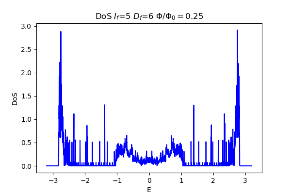
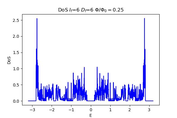
Figure 3: The density of states for Sierpinski carpet with $I_{f}=5$, $D_{f}=6$ and $D_{f}=I_{f}=6$ (maximum number of iterations for the square with size $3^{6}\times 3^{6}$), $\Phi/\Phi_{0}=0.25$. A gap appears in the middle of the spectrum for $I_{f}=6$, in comparison with $I_{f}=5$.

III.2 Hall conductivity

In order to calculate Hall conductivity, we use the approach from Refs. Garcila_etal2015, ; ShengjunEdo2016, . The method is based on the so called Kubo-Bastin formula:

$$\sigma_{\alpha\beta}=\frac{i\hslash e^{2}}{A}\int^{+\infty}_{-\infty}d\epsilon f(\epsilon)\operatorname{Tr}\langle v_{\alpha}\delta(\epsilon-H)v_{\beta}\frac{dG^{+}(\epsilon)}{d\epsilon}$$

$$-v_{\alpha}\delta(\epsilon-H)v_{\beta}\frac{dG^{-}(\epsilon)}{d\epsilon}\rangle$$

where $A$ is the area of the sample, $f(\epsilon)=\frac{1}{\exp{(\epsilon-\mu)/T}}$ is the Fermi-Dirac distribution, $T$ is the temperature, $\mu$ is the chemical potential, $v_{\alpha}$ is $\alpha$ component of velocity operator, $G^{\pm}=1/(\epsilon-H\pm i\eta)$ are the Green’s functions. In this formula we also average over random samplings as we did for the density of states. We can expand Green’s functions and delta function in Chebyshev polinomials and then for the conductivity we obtain:

$$\sigma_{\alpha\beta}=\frac{4\hslash e^{2}}{\pi A}\frac{4}{\Delta E^{2}}\int^{1}_{-1}d\tilde{\epsilon}\frac{f(\tilde{\epsilon})}{(1-\tilde{\epsilon}^{2})^{2}}\sum_{m,n}\Gamma_{nm}(\tilde{\epsilon})\mu^{\alpha\beta}_{m,n}(H)$$ (2)

where $\tilde{\epsilon}$ is rescaled energy within $[-1,1]$, $\Delta E$ is the energy range of spectrum, $\mu^{\alpha\beta}_{m,n}(H)$ and $\Gamma_{nm}(\tilde{\epsilon})$ are described by the following formulas:

$$\Gamma_{nm}(\tilde{\epsilon})=T_{m}(\tilde{\epsilon})(\tilde{\epsilon}-in\sqrt{1-\tilde{\epsilon}^{2}}e^{in\arccos(\tilde{\epsilon})})$$

$$+T_{n}(\tilde{\epsilon})(\tilde{\epsilon}+im\sqrt{1-\tilde{\epsilon}^{2}}e^{-im\arccos(\tilde{\epsilon})})$$

and

$$\mu^{\alpha\beta}_{m,n}(H)=\frac{g_{m}g_{n}}{(1+\delta_{n0})(1+\delta_{m})}$$

We use Jackson kernel $g_{m}$ to smooth Gibbs oscillations due to truncation of the expansion in Eq. (2) Garcila_etal2015 .

Our results for $\sigma_{xy}$ are shown in Fig. 4. The Hall conductivity was calculated for $\Phi/\Phi_{0}=0.25$, $D_{f}=6$ and $I_{f}=0,4,5,6$.

The Kubo-Bastin formula is derived under very general assumptions and can be used to study linear response for any Hamiltonian within single particle approximation. The only restriction of the formula is that it neglects the interelectron interactions. For example, the Kubo-Bastin formula was successfully applied to systems with irregularities, such as disordered systems Garcila_etal2015 , which also lack translational symmetry, and it can be used for fractals as well.

The Hall conductivity behaves similarly to the DoS pictures. The differences between $I_{f}=0$ and $I_{f}=4$ are quite small, although there are fluctuations in the case of $I_{f}=4$. The structure is similar, there are plateaus, which correspond to relatively small values of DoS, in the middle of the spectrum and between peaks. These plateaus are an indication of relation between Hall conductivity and topological invariants: Hall conductivity takes value of $e^{2}/h$ multiplied by integer (this integer equals to Chern number). One can see a clear transition at $I_{f}=5$ iterations. The plateaus in the middle of the spectrum are vanished at $I_{f}=5$ and fluctuations become much stronger.

The picture of Hall conductivity for $I_{f}=D_{f}=6$ demonstrates a completely different behaviour. We can compare these results to Chern numbers calculated in Ref. Brzezetal2018, (Fig. 3(c) in that article) for $I_{f}=D_{f}=4$. In general, Hall conductivity looks similar to Chern numbers, however, there are more fluctuations and peaks that are absent in the behaviour of Chern numbers. One can also notice that plateaues appear on the scale $1.5e^{2}/h$, not $e^{2}/h$, which would correspond to values of Chern number on these energies. The exact plateaus of Chern numbers are located on the energies $E=-1.5\ldots-0.9$ and $E=0.9\ldots 1.5$, almost quantized region is located around $\pm 2.5$ with the width of the order of $0.1$. These regions are highlighted in Fig. 4(d).

There are two regions which correspond to quantized Chern number, around $E=\pm 1$. These regions occur after smearing of peaks in smaller iteration depths $I_{f}$. From the previous plateaus there remain only small parts around $E=\pm 2.5$ and a part of region around $E=\pm 1$, these regions correspond to almost quantized Chern number. It is interesting that regions around $E=\pm 1$ with quantized Chern numbers are not flat plateaus. This was checked for different numbers of random samples and fluctuations were stable. The central gap in DoS corresponds to conductivity $\sigma_{xy}=0$, as well as the Chern number, which is equal to $0$. Therefore, we can conclude that the relation between Chern numbers and Hall conductivity does not hold in non-integer dimensions, although there are similarities in their behaviour.

We also added disorder to the sample by deleting random sites. The results are shown in Fig. 5, where we deleted around $20\%$ of sites in the sample. We see that DoS as well as Hall conductivity are stable with respect to the disorder. Moreover, one can see even less fluctuations on the pictures in comparison with Fig. 4. Thus, we can conclude that fractals are stable to disorder, like systems with integer dimensions.

Particularly this result could be expected, since holes in a fractal sample already could be seen as a kind of disorder. Therefore additional disorder should not effect physical properties unless this disorder is large enough. However, there are subtleties since exact scaling symmetry on all scales is important for correct approximation of the fractal.

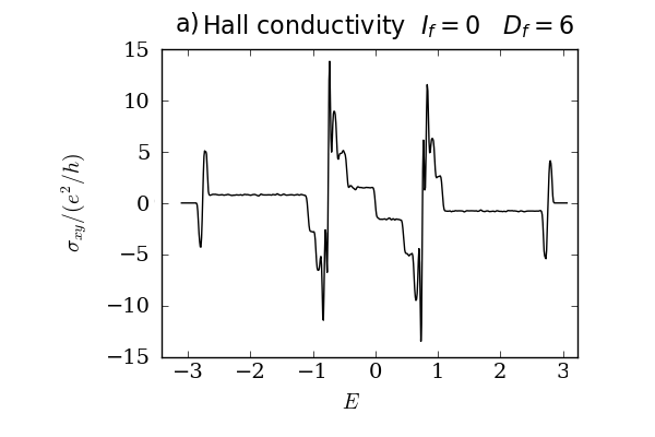
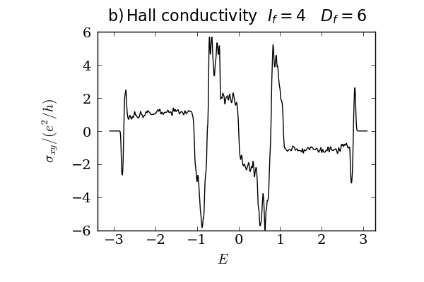
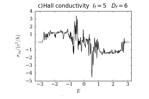
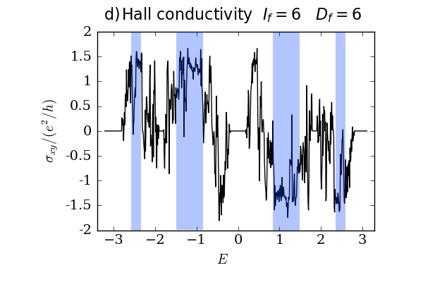
Figure 4: The Hall conductivity for different iterations of Sierpinski carpet in a square of the size $3^{D_{f}}\times 3^{D_{f}}$ and $D_{f}=6$ ($\Phi/\Phi_{0}=0.25$): a) is $I_{f}=0$ iteration, b) is $I_{f}=4$ iterations, c) is $I_{f}=5$ iterations, d) is $I_{f}=6$ iterations. As in the Fig. 2, the differences between a) and b) are small, only small fluctuations are added in b). Picture c) demonstrates transition to another phase, picture d) is very different from previous cases, the regions of quantized Chern numbers are shown by blue.

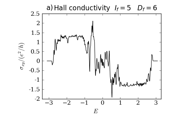
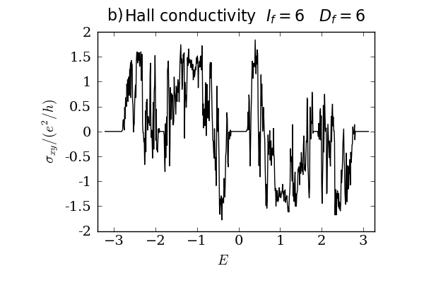
Figure 5: The Hall conductivity for Sierpinski carpet with additional disorder in a square of the size $3^{D_{f}}\times 3^{D_{f}}$ and $D_{f}=6$ ($\Phi/\Phi_{0}=0.25$): a) is $I_{f}=5$ iteration, b) is $I_{f}=6$ iterations. Approximately $20\%$ sites are deleted. There are no visible differences from the Fig. 4

III.3 Quasi-eigenstates

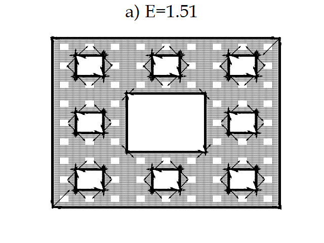
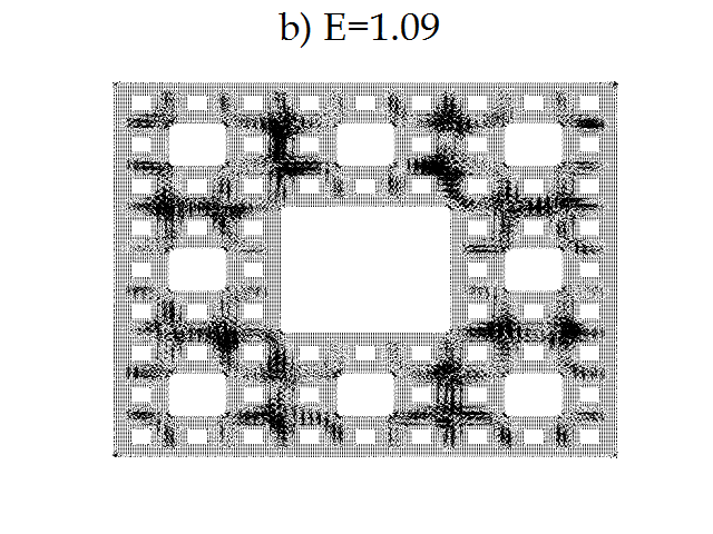
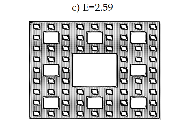
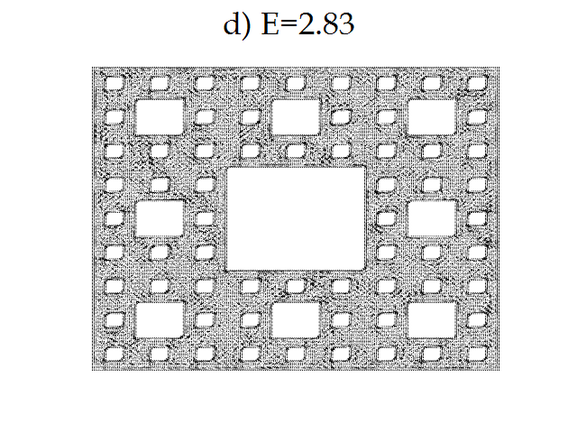
Figure 6: Quaisi-eigenstates for Sierpinski carpet with size $3^{D_{f}}\times 3^{D_{f}}$ with $D_{f}=5$ and $I_{f}=3$ iterations. Examples of edge states are on the left: picture a) $E=1.51$, picture c) $E=2.59$. Examples of bulk states are on the right: picture b) $E=1.09$, picture d) $E=2.83$

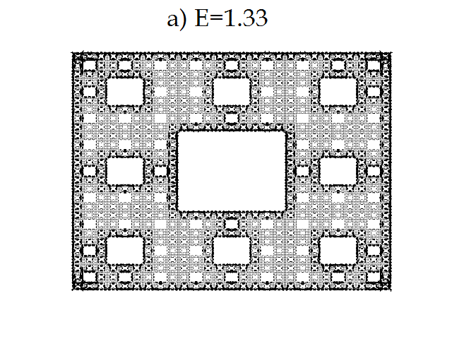
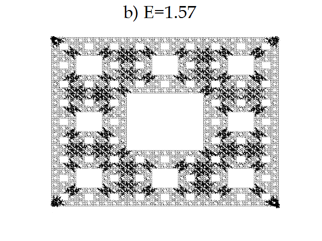
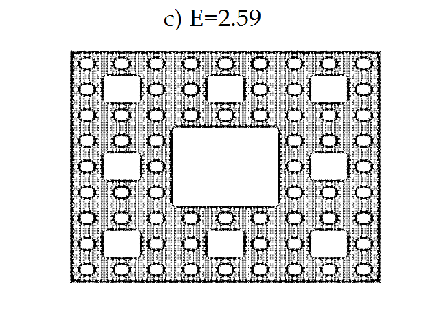
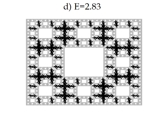
Figure 7: Quaisi-eigenstates for Sierpinski carpet with size $3^{D_{f}}\times 3^{D_{f}}$ with $D_{f}=5$ and $I_{f}=3$ iterations. Examples of edge states are on the left: picture a) $E=1.33$, picture c) $E=2.59$. Examples of bulk states are on the right: picture b) $E=1.57$, picture d) $E=2.83$ .

It is known that the edge states in quantum Hall systems are closely related to their topological properties Prange1987 ; Halperin1982 ; Hatsugai1993 . Occurrence of the edge states corresponds to quantized Chern numbers (bulk-edge correspondence). Therefore it is natural to assume that transitions with increasing $I_{f}$ in DoS and Hall conductivity will be seen in the edge states as well. To explore this question we calculated quasi-eigenstates for Sierpinski carpet. Quasi-eigenstates and probability current were calculated by the same method of averaging Shengjun2010 . For the probability current, we use the formula Hornberger2002 :

$$\mathbf{j}=\operatorname{Re}(\psi^{*}\mathbf{v}\psi)=\frac{\hbar}{m_{e}}\operatorname{Im}(\psi^{*}\nabla\psi)-\frac{q}{m_{e}}\mathbf{A}|\psi|^{2}$$ (3)

First, let us take a look at states corresponding to plateaus and peaks for some iterations with enough holes, but with regular behaviour of Hall conductivity. For more readable pictures we used samples with size $D_{f}=5$. Examples of bulk and edge states for $I_{f}=3$ iterations are shown in Fig. 6. Edge states, which are shown on the left side of picture, correspond to energies $E=1.51$ and $E=2.59$. Bulk states, which are shown on the right side of picture, correspond to energies $E=1.09$ and $E=2.83$. Edge states correspond to plateaus in Hall conductivity and bulk states correspond to slopes of peaks. We see that edge states can be localized along holes on different scales i.e. only the central hole, holes of the second iteration and the central hole, all holes up to the third iteration and so on.

Examples of bulk and edge states for $I_{f}=5$ iterations (i.e. fractal with maximum depth) are shown in Fig. 7. Edge states, which are shown on the left side of the picture, correspond to energies $E=1.33$ and $E=2.59$. Bulk states, which are shown on the right side of the picture, correspond to energies $E=1.57$ and $E=2.83$. Edge states correspond to quantized and almost quantized Chern number. There is a reminiscence of this quantization in Hall conductivity.

We see that the edge states in the full fractal differ from the edge states in Fig. 6. In the sample with $I_{f}=3$ iterations, the current is localized along borders in a homogeneous pattern, there are just lines of currents along the edges. However, in the full fractal, the current has a more complex pattern, for example, it can be localized along small holes, which are close to an edge. This deformation of edge current can be a reason of absence of plateaus in Hall conductivity even for regions with quantized Chern number. We also see that bulk states in a sample with $I_{f}=5$ iterations demonstrate more symmetric behaviour. This is, obviously, the manifestation of full scaling symmetry of a fractal.

We see that for the energies $E=1.33$ and $E=2.59$, which is in the region of almost quantized and quantized Chern number, the edge states remain to be well-defined. However, some part of plateaus of the previous iterations with the edge states become bulk states. We also see that some bulk states in different iterations have similar localization properties. Accordingly, we can assume that there are states with different effective scales. Some states spread over the rougher structure of a sample, some states sit only around smaller holes.

We have made calculations for various energies and they all follow the described pattern. We see that the quasi-eigenstates corresponding to the quantized Hall conductivity are localized along the edges for iterations smaller than $I_{f}=4$ (with maximum possible number of iterations equal to $D_{f}=5$). It is also worth noticing that all edges, namely, the edges of the sample and the edges of the holes can contribute to quasi-eigenstates. For the most of quasi-eigenstates which have been calculated for various energies in the case of $I_{f}=5$ and $D_{f}=5$, there was no obvious domination of edge states.

We observe that the same transition, which already was observed in DoS and Hall conductivity, manifests in quasi-eigenstates, when the number of iterations is one less than the possible number of iterations. In the case of bulk states, it manifests as a more symmetric picture of the current. In the case of edge states, it manifests as a more complex localization along the edges, so that some edge states become localized along smaller holes, which are close to an edge.

IV Summary

We see that with increasing the depth of a fractal the quantization of Hall conductivity disappears. However, there is some reminiscence of topological nature of quantization, namely some plateaus remain. We also see that for Sierpinski carpet the relation between topological invariants such as Chern numbers and Hall conductivity does not work, contrary to the case of integer dimensions. The calculated conductivity is not proportional to the Chern number, but follows a similar pattern. One can speculate about possible reasons of it.

At first, the formula, which calculates Chern number through projectors, was proven to be properly defined only for systems with translational invariance Kitaev2006 . Even if the formula works for fractals, it may be that one needs to calculate Hall conductivity and Chern numbers in the thermodynamic limit. Another reason can be related to difficulties with defining edge and bulk states. Some of the edge states are localized along inner holes. These states become closer to bulk states at maximal depth, so we cannot saywhether it is the localization along the edges or localization on small inhomogeneities. Edge states along large holes also become localized not only along edges, but also along small holes around an edge. These possible effects require future investigation.

We considered different iterations $I_{f}$ of Sierpinski carpet on a fixed rectangular sample with size $3^{D_{f}}\times 3^{D_{f}}$. We observed that there is a transition between two different regimes, which occurs when $I_{f}=D_{f}-1$. This transition can be seen in density of states, Hall conductivity and quasi-eigenstates. In the case of quaisi-eigenstates, the edge states mostly become bulk states when $I_{f}$ is increased. This result can be explained by the effective dimension. If the number of holes is finite, then the effective dimension of a sample is integer rather than fractional. The transition occurs when holes in a sample are dense enough and the effective dimension of the sample becomes non-integer.

Edge states can be localized along the borders of all holes of various scales, not only the edges of the sample. There is no big difference in amplitude of currents for different holes. Edge states can still be seen for a full fractal, however, they change their localization behavior. Additional holes along the edges increase effective localization width. Therefore, one can speculate that if a state is localized around small holes and these holes are dense enough, there could be a transition from edge state to a bulk state.

When this work was finished the preprint Fritz2019 appeared which treated a similar problem but in a technically different way (it was based on Landauer formula rather than Kubo-Bastin formula and did not include an analysis of edge states). Qualitatively, parts of our conclusions are similar to these obtained in that paper.

V Acknowledgements

We are thankful to Tom Westerhout for the helpful discussions. This work was supported by the National Science Foundation of China under Grant No. 11774269 and by the Dutch Science Foundation NWO/FOM under Grant No. 16PR1024 (S.Y.), and by the by the JTC-FLAGERA Project GRANSPORT (M.I.K.). Support by the Netherlands National Computing Facilities foundation (NCF), with funding from the Netherlands Organisation for Scientific Research (NWO), is gratefully acknowledged.

References

- (1) S. Havlin and D. Ben-Avraham, Diffusion in disordered media, Advances in Physics 36, 695 (1987).
- (2) L. Pietronero and E. Tosatti (Editors), Fractals in physics. (Elsevier, Amsterdam, 1986).
- (3) J. Feder, Fractals (Plenum Press, New York, 1988).
- (4) E. Domany, S. Alexander, D. Bensimon, and L. Kadanoff, Solutions to the Schrödinger equation on some fractal lattices, Phys. Rev. B 28, 3110 (1983).
- (5) M. Polini, F. Guinea, M. Lewenstein, H. C. Manoharan, and V. Pellegrini, Artificial honeycomb lattices for electrons, atoms and photons, Nature Nanotechnology 8, 625 (2013).
- (6) M. Gibertini, A. Singha, V. Pellegrini, M. Polini, G. Vignale, A. Pinczuk, L. N. Pfeiffer, and K. W. West, Engineering artificial graphene in a two-dimensional electron gas, Phys. Rev. B 79, 241406(R) (2009).
- (7) J. Shang, Y. Wang, M. Chen, J. Dai, X. Zhou, J. Kuttner, G. Hilt, X. Shao, J. M. Gottfried, and K. Wu, Assembling molecular Sierpinski triangle fractals, Nature Chemistry 7, 389 (2015).
- (8) S. N. Kempkes, M. R. Slot, S. E. Freeney, S. J. M. Zevenhuizen, D. Vanmaekelbergh, I. Swart, and C. Morais Smith, Design and characterization of electrons in a fractal geometry, Nature Physics 15, 127 (2018).
- (9) E. van Veen, S. Yuan, M. I. Katsnelson, M. Polini, and A. Tomadin, Quantum transport in Sierpinski carpets, Phys. Rev. B 93, 115428 (2016).
- (10) E. van Veen, A. Tomadin, M. Polini, M. I. Katsnelson, and S. Yuan, Optical conductivity of a quantum electron gas in a Sierpinski carpet, Phys. Rev. B 96, 235438 (2017).
- (11) Z.-G. Song, Y.-Y. Zhang, and S.-S. Li, The topological insulator in a fractal space, Appl. Phys. Lett. 104, 233106 (2014).
- (12) T. Westerhout, E. van Veen, M. I. Katsnelson, and S. Yuan, Plasmon confinement in fractal quantum systems, Phys. Rev. B 97, 205434 (2018).
- (13) D. Sticlet and A. Akhmerov, Attractive critical point from weak antilocalization on fractals, Phys. Rev. B 94, 161115(R) (2016).
- (14) A. Kosior and K. Sacha, Localization in random fractal lattices, Phys. Rev. B 95, 104206 (2017).
- (15) M. Brzezinska, A. M. Cook, and T. Neupert, Topology in the Sierpinski-Hofstadter problem Phys. Rev. B 98, 205116 (2018).
- (16) A. Agarwala, S. Pai, and V. B. Shenoy, Fractalized Metals ArXiv e-prints (2018), arXiv:1803.01404 [cond-mat.dis-nn].
- (17) B. Pal, W. Wang, S. Manna, A. E. B. Nielsen, Anyons and Fractional Quantum Hall Effect in Fractal Dimensions ArXiv e-prints (2019), arXiv:1907.03193 [cond-mat.str-el].
- (18) S. Pai, A. Prem, Topological states on fractal lattices ArXiv e-prints (2019), arXiv:1907.01558 [cond-mat.mes-hall].
- (19) A. K. Golmankhaneh, Statistical Mechanics Involving Fractal Temperature Fractal Fract. 3(2), 20 (2019).
- (20) I. Akal, Entanglement entropy on finitely ramified graphs Phys. Rev. D 98, 106003 (2018).
- (21) B. Pal and K. Saha, Flat bands in fractal-like geometry Phys. Rev. B 97, 195101 (2018)
- (22) A. Nandy and A. Chakrabarti, Engineering slow light and mode crossover in a fractal-kagome waveguide network Phys. Rev. A 93, 013807 (2016).
- (23) A. Nandy, B. Pal and A. Chakrabarti, Flat band analogues and flux driven extended electronic states in a class of geometrically frustrated fractal networks Journal of Physics: Condensed Matter 27(12), 125501 (2015).
- (24) D. J. Thouless, M. Kohmoto, M. P. Nightingale, and M. den Nijs, Quantized Hall conductance in a two-dimensional periodic potential, Phys. Rev. Lett. 49, 405 (1982).
- (25) D.-C. Tran, A. Dauphin, N. Goldman, and P. Gaspard, Topological Hofstadter insulators in a two-dimensional quasicrystal, Phys. Rev. B 91, 085125 (2015).
- (26) Y. E. Kraus and O. Zilberberg, Topological Equivalence between the Fibonacci Quasicrystal and the Harper Model, Phys. Rev. B 91, 085125 (2015).
- (27) J. Bellissard Gap Labelling Theorems for Schrödinger Operators. In: M. Waldschmidt, P. Moussa, JM. Luck, C. Itzykson (eds) From Number Theory to Physics. Springer, Berlin, Heidelberg (1992).
- (28) E. Prodan Disordered topological insulators: a non-commutative geometry perspective, J. Phys. A: Math. Theor. 44, 239601 (2011).
- (29) J. Bellissard, A. van Elst, and H. Schulz‐Baldes The noncommutative geometry of the quantum Hall effect, J. Math. Phys. 35, 5373 (1994).
- (30) G. B. Halász, T. H. Hsieh, and L. Balents, Fracton topological phases from strongly coupled spin chains, Phys. Rev. Lett. 109, 116404 (2012).
- (31) T. Devakul, Y. You, F. J. Burnell, S. L. Sondhi, Fractal symmetric phases of matter SciPost Phys. 6, 007 (2019).
- (32) B. I. Halperin, Quantized Hall conductance, current-carrying edge states, and the existence of extended states in a two-dimensional disordered potential Phys. Rev. B 25, 2185 (1982).
- (33) Y. Hatsugai, Chern number and edge states in the integer quantum Hall effect Phys. Rev. Lett. 71, 3697 (1993).
- (34) R. S. K. Mong and V. Shivamoggi, Edge states and the bulk-boundary correspondence in Dirac Hamiltonians Phys. Rev. B 83, 125109 (2011).
- (35) A. A. Iliasov, M. I. Katsnelson, and S. Yuan, Power-law energy level spacing distributions in fractals, Phys. Rev. B 99, 075402 (2019).
- (36) A. Hernando, M. Sulc, and J. Vanicek, Spectral properties of electrons in fractal nanowires ArXiv e-prints (2019), arXiv:1907.01558 [cond-mat.mes-hall]
- (37) K. Machida and M. Fujita, Quantum energy spectra and one-dimensional quasiperiodic systems, Phys. Rev. B 34, 7367 (1986).
- (38) A. Hams and H. De Raedt, Fast algorithm for finding the eigenvalue distribution of very large matrices, Phys. Rev. E 62, 4365 (2000).
- (39) S. Yuan, H. De Raedt, and M. I. Katsnelson, Modeling electronic structure and transport properties of graphene with resonant scattering centers Phys. Rev. B 82, 115448 (2010).
- (40) J. H. Garcia, L. Covaci, and T. G. Rappoport, Real-space calculation of the conductivity tensor for disordered topological matter Phys. Rev. Lett. 114, 116602 (2015).
- (41) S. Yuan, E. van Veen, and M. Katsnelson, R. Roldan, Quantum Hall effect and semiconductor-to-semimetal transition in biased black phosphorus, Phys. Rev. B 93, 245433 (2016).
- (42) D. R. Hofstadter, Energy levels and wave functions of Bloch electrons in rational and irrational magnetic fields Phys. Rev. B 14, 2239 (1976).
- (43) R. E. Prange and S. M. Girvin (Editors), The quantum Hall effect (Springer, Berlin, 1987).
- (44) K. Hornberger, U. Smilansky, Magnetic edge states Physics Reports 367, 249 (2002) .
- (45) A. Kitaev, Anyons in an exactly solved model and beyond Annals of Physics 321, 2–111 (2006).
- (46) M. Fremling, M. van Hooft, C. Morais Smith, and L. Fritz, A Chern insulator in ln(8)/ln(3) dimensions arXiv:1906.07387 [cond-mat.str-el].