Searching for correlations in Gaia DR2 unbound star trajectories

Abstract

Scattering events with compact objects are expected in the primordial black hole (PBH) cold dark matter (CDM) scenario due to close encounters between stars and PBH in the dense environments of dwarf spheroidals. We develop a Bayesian framework to search for correlations among Milky Way stellar trajectories and those of globular clusters and dwarf galaxies in the halo, and other nearby galaxies. We apply the method to a selection of hypervelocity stars (HVS) and globular clusters from Gaia DR2 catalog, and known nearby (mostly dwarf) galaxies with full phase-space and size measurements. We report positive evidence for trajectory intersection $\sim$20–40 Myr ago of up to 2 stars, depending on priors, with the Sagittarius dwarf Spheroidal (dSph) galaxy when assuming Marchetti et al. (2019) distance estimates. We verify that the result is compatible with their evolutionary status, setting a lower bound for the stellar age of $\sim$100 Myr. However, such scattering events are not confirmed when assuming Anders et al. (2019) distance estimates. We discuss shortcomings related to present data quality and future prospects for detection of HVS with the full Gaia catalog and Sagittarius dSph.

1 Introduction

The hierarchical structure formation scenario assumes that large galaxies are formed by mergers of smaller ones, which bring in both gas (hydrogen), stars and dark matter (DM). These smaller structures, generically called dwarf galaxies, orbit around the larger galaxy and interact with it. Some appear tidally disrupted by previous crossings through the disk and are elongated, and others are still approaching it and have more or less spherical shape. All this substructure have large mass-to-light ratios, in some cases larger than 1000, making them extremely difficult to detect in the sky. Their numbers were predicted, within the cold dark matter scenario, to be large, hundreds to thousands of objects orbiting each large galaxy. However, only about a dozen had been observed until SDSS and DES discovered several tens of them (Drlica-Wagner et al., 2015; Newton et al., 2018; Simon et al., 2019), solving the so-called substructure problem when extrapolated to the whole sky.

The low surface brightness of dwarf galaxies could be explained in the PBH CDM scenario (García-Bellido, 2017) due to the loss of stars via close encounters with massive primordial black holes comprising the dark matter halos of all galaxies. In this scenario, stars in the shallow potential wells of dwarf galaxies are more likely to get slingshot away due to close encounters with DM black holes, acquiring velocities in the hundreds to thousands of km/s (Clesse & García-Bellido, 2017). Such hypervelocity stars (HVS), likely unbound to the Milky Way potential, should travel across the sky and their trajectories should point back to the dSph from which they originate. High-velocity stars are also found in the core of globular clusters (GC) (Lützgendorf et al., 2012), which may indicate a population of PBH, and also in this case some of them may acquire a velocity above the escape threshold (Clesse & García-Bellido, 2017).

In this paper we develop a Bayesian framework for the detection of such close encounters via the correlation of stellar trajectories in Gaia DR2 catalog (Gaia Collaboration et al., 2016, 2018a) with trajectories of dwarf and other nearby galaxies, and GC. If massive black holes are indeed responsible for the depletion of stars from dwarf galaxies, it is expected that a few slingshot events must have happened in the last 100 million years inside dwarf galaxies in the Milky Way. In particular, since the probability of events is proportional to the density of the dwarf galaxy, one expects the most massive ones to be the source of HVS. Unfortunately, Gaia has limited resolution for distant stars, and only those relatively close to the Sun are measured with sufficient accuracy in 6D phase space (we consider stars up to $\sim$13 kpc).

Recently, Marchetti et al. (2019) found that some of the observed HVS were not pointing away from the center of the Milky Way, as was naively expected, but rather towards the disk, as if they had originated in the halo of our galaxy. Furthermore, Hattori et al. (2018) reported one star whose orbit has non-negligible probability of having passed near the Large Magellanic Cloud in the past. This prompted us to explore the possible origin of HVS and whether they could originate in the dSph that orbit around the MW within a radius of several tens of kiloparsecs, and which could have been travelling for several tens of millions of years from their sources and velocities up to ten times larger than typical stellar velocities in the halo.

We compute the close encounter evidence between HVS and Milky Way GC, dwarf, and nearby galaxies studying the posterior distribution of an impact parameter defined upon phase-space and size information. The evolutionary status of HVS scattering candidates is further analyzed based to their Hertzsprung–Russell (HR) diagram to confirm that their expected age is consistent with having travelled over typically large distances.

In section 2 we illustrate our Gaia DR2 HVS catalog, and the data selection for Milky Way GC and nearby galaxies discussing distribution and kinematic properties properties of each selection. In section 3 we outline our Bayesian methodology to evaluate the scattering evidence between HVS and compact objects in GC or nearby galaxies. In section 4 we give our results. We conclude in section 5. In appendix A we discuss results based on an alternative stellar selection than the one considered throughout the main paper. In appendix B we define our Galactocentric reference frame. In appendix C we provide references for the selected GC and galaxies, as well as orbit data for Sagittarius dSph and HVS compatible with having crossed its trajectory.

2 Data

2.1 Hyper-velocity stars

Our reference catalog is Gaia DR2 (Gaia Collaboration et al., 2016, 2018a), an all sky survey consiting of more than 1.3 billion stars. It contains accurate accurate positions ($\alpha$, $\delta$), proper motions ($\mu_{\alpha*}$,$\mu_{\delta}$), parallax ($\omega$), radial velocity, magnitudes and colors for the bright end, for $\sim 7$ million stars. We base our analysis on the 7183262 stars selection provided by Marchetti et al. (2019), established with the following quality cuts (see also Gaia DR2 documentation for more information about variables description):

• astrometric_gof_al $<3$.

• astrometric_excess_noise_sig $\leq 2$.

• $-0.23\leq$ mean_varpi_factor_al $\leq 0.32$.

• visibility_periods_used $>8$.

• rv_nb_transits $>5$.

We further clean the sample:

• Selecting heliocentric total velocities in the Galactic rest frame large enough compared to their uncertainties $v-\sigma_{v}\gtrsim 500$ km/s, to mitigate errors in the Galactic absolute velocity.

• Removing potentially spurious radial velocities (Boubert et al., 2019).

Marchetti et al. (2019) provides for each star the probability $P_{\rm ub}$ of being unbound to the Milky Way potential. Our final selection of 1649 stars takes into account this information and further photometric and astrometric quality cuts (Schönrich et al., 2019):

• $P_{\rm ub}>0.5$.

• Color cut $G_{\rm BP}-G_{\rm RP}<1.5$ mag.

• Magnitude cut $G<14.5$ mag, and $G,G_{\rm BP},G_{\rm RP}>0$ mag.

• BP-RP excess flux factor cut $1.172<E_{\rm bprp}<1.3$.

• astrometric_excess_noise $<1$.

See appendix A for an alternative stellar selection.

We consider distance estimates given in Marchetti et al. (2019). The catalog does not include systematic errors on parallax measurements, and it sets a large scale length in the distance prior for likely distant stars that may overestimate distances. To overcome these shortcomings, we also consider the more recent Anders et al. (2019) work that improves the accuracy of extinction and effective temperature estimates provided with Gaia DR2 by combining its astrometric and photometric measurements with external photometric catalogs. In particular, the related distance catalog includes errors induced by a parallax zero-point offset. We find that Marchetti et al. (2019) distances are systematically larger on average by roughly a factor of 2 than Anders et al. (2019) estimates for distant stars. The disagreement increases even up to an order of magnitude for stars whose distance is estimated to be $\lesssim 2$ kpc by Anders et al. (2019), whereas this latter catalog agrees well with other computations (Bailer-Jones et al., 2018; Schönrich et al., 2019) within this range. Probabilities $P_{\rm ub}$ used for our selection rely on Marchetti et al. (2019) distances, but evaluating $P_{\rm ub}$ based on Anders et al. (2019) is beyond the scope of the present work. Since $P_{\rm ub}$ does not enter in following computations, comparing results based on the two different distance estimates still provides a consistency check.

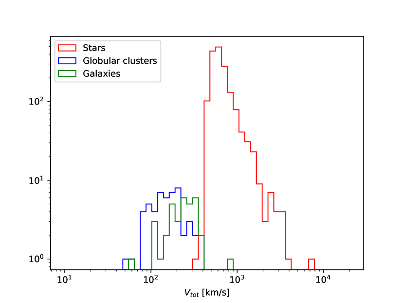
Figure 1: Total velocities in Galactocentric coordinates for our selection of stars, globular clusters and galaxies.

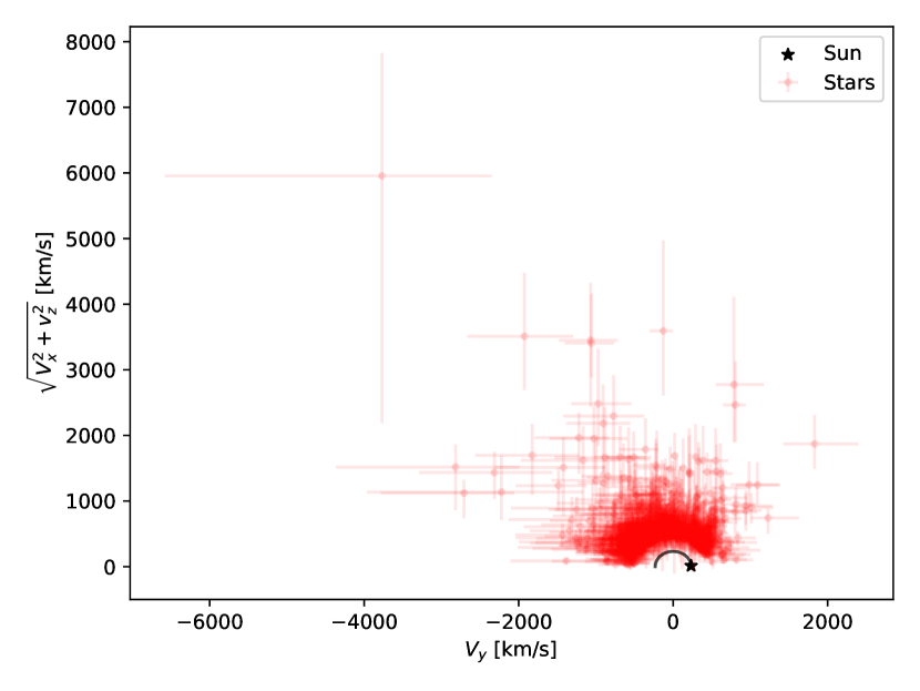
Figure 2: Toomre diagram in terms of Galactocentric Cartesian velocities for our HVS selection. All HVS are above the black semi-circle centered at the origin and of radius given by the Sun (black star) $V_{y}$ component.

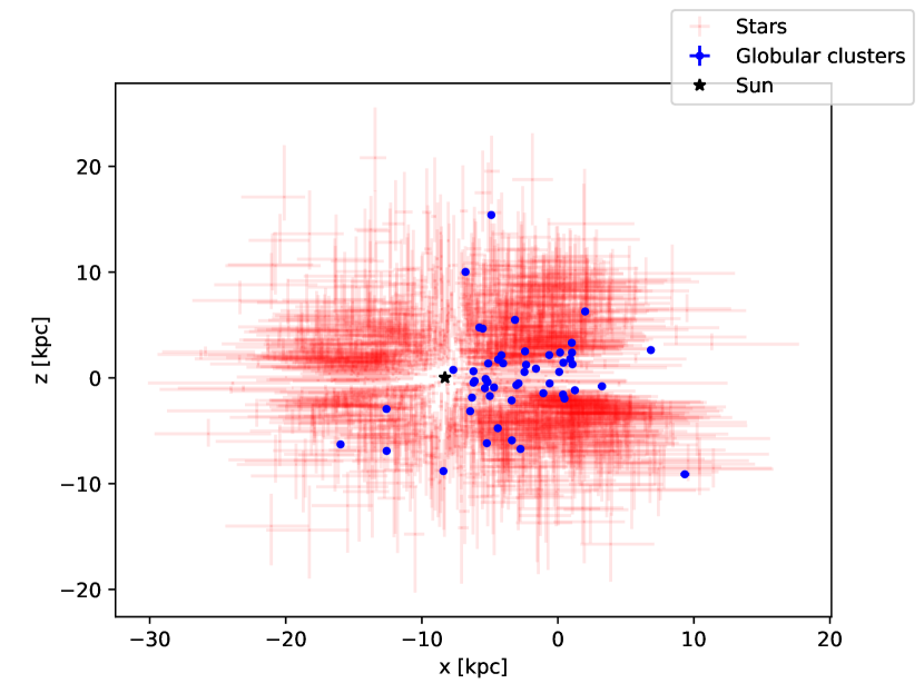
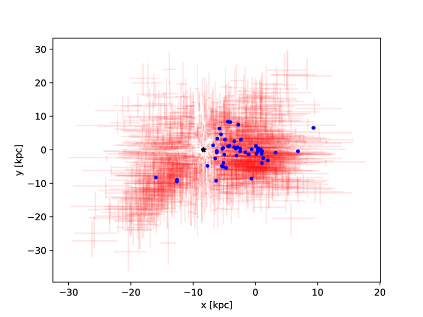
Figure 3: Galactocentric positions for stars and globular clusters. Error bars $\lesssim 3\%$ for GC are smaller than markers (the latter are not representative of objects extension).

Figure 1 shows that most of our HVS selection is characterized by total Galactocentric velocities $V_{tot}\sim\mathcal{O}(10^{3})$ km/s. For details about our coordinates system see appendix B. Figure 2 shows the Toomre diagram with the Galactocentric Cartesian $V_{y}$ component on the abscissa, and the $\sqrt{V_{x}^{2}+V_{z}^{2}}$ component on the ordinate. Here and afterwards error bars indicates 68% confidence intervals. The diagram is populated only above a semi-circle centered at the origin and of radius given by the Sun $V_{y}$ component, suggesting that we select a population of halo stars (e.g., Bonaca et al., 2017). Figure 3 shows Galactocentric positions with error bars dominated by uncertainties on distances from the Sun.

2.2 Globular clusters and galaxies

We select 52 globular clusters (GC) identified in the Gaia DR2 catalog (Gaia Collaboration et al., 2018b) that report both full phase-space and radius, defined as the maximum radius at which proper-motion members are found.

We select all galaxies for which we can match position and half-light radius (measured along major axes) given by McConnachie (2012) with peculiar motions of identified dwarf Milky Way satellite galaxies in Gaia DR2 (Fritz et al., 2018). We also include Antlia II (Torrealba et al., 2019) and Andromeda (velocity from van der Marel et al., 2012). In the latter case we retrieve the optical major-axis from the SIMBAD database (Wenger et al., 2000), also used to get sizes and velocities of the large (LMC) and small (SMC) Magellanic clouds that we combine with positions listed in McConnachie (2012). This gives a total of 35 galaxies.

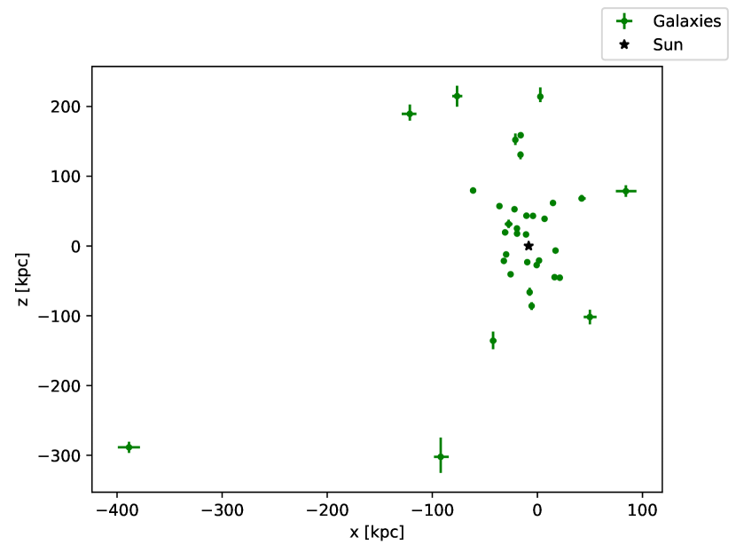
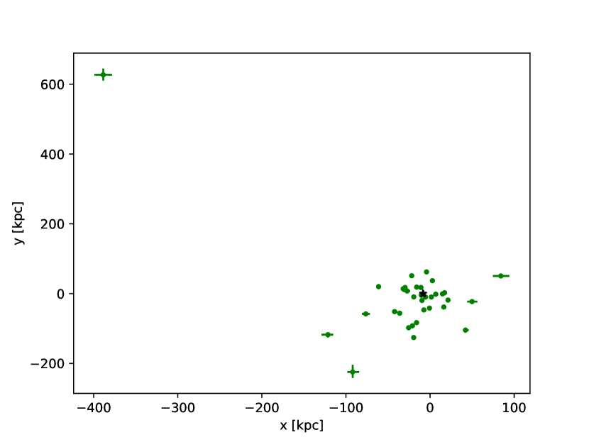
Figure 4: Galactocentric positions for galaxies. The further galaxy is Andromeda. Marker size (for some object larger that error bars) is not representative of object extension.

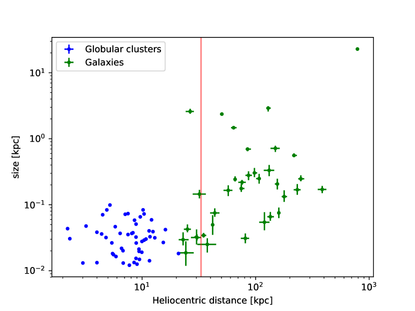
Figure 5: Heliocentric distance and size for GC and galaxies. The vertical line corresponds to the further HVS; the largest object within this distance is Sagittarius dSph, placed at coordinates $(26\pm 2,2.6\pm 0.2)$ kpc.

Figure 1 shows total Galactocentric velocities $V_{tot}\sim\mathcal{O}(10^{2})$ km/s both for GC and galaxies. Figures 3 and 4 show GC and galaxy positions, respectively. We verified that the asymmetric GC distribution, concentrated between the Sun and the galactic Center is also present in the full catalog and not only in our selection (note the lack of GC in the upper quadrants for objects with $x<x_{\sun}\approx-8.3$ kpc). Figure 5 shows heliocentric distances and sizes in terms of radii defined above. GC are characterized by sizes $\mathcal{O}(10)$ – $\mathcal{O}(100)$ pc, while galaxies show a larger variation because we include objects of different types, ranging from dwarfs with radius $\sim\mathcal{O}(10)$ pc to large galaxies such as Andromeda with major semi-axis $\sim 23$ kpc. Most galaxies reach distances further than our HVS selection.

Further details about the selected objects are given in appendix C.

3 Methodology

3.1 Trajectories

Orbits are integrated using the gala software library (Price-Whelan, 2017). We use its default Milky Way potential model based on four components. Below $G$ indicates the gravitational constant, $r_{s}$ is the radial distance in Galactocentric spherical coordinates, $r_{c}$ and $z_{c}$ are the radial distance and height, respectively, in Galactocentric cylindrical coordinates. The nucleus and bulge follow a Hernquist potential for a spheroid (Hernquist, 1990):

$$\phi(r_{s})=-\frac{Gm}{r_{s}+a}\;.$$ (1)

The disk follows a Miyamoto-Nagai profile (Miyamoto & Nagai, 1975; Bovy, 2015):

$$\phi(r_{c},z_{c})=-\frac{Gm}{\sqrt{r_{c}^{2}+\left(a+\sqrt{z_{c}^{2}+b^{2}}\right)^{2}}}\;.$$ (2)

The halo follows a spherical Navarro-Frenk-White (NFW) profile: (Navarro et al., 1996).

$$\phi(r_{s})=-\frac{Gm}{r_{s}}\ln\left(1+\frac{r_{s}}{a}\right)\;.$$ (3)

We use the same parameters as in Marchetti et al. (2019), summarized in table 1. In the PBH CDM scenario the inner part of the halo is better described by an Einasto profile (Einasto, 1965), but this only affects the dynamics close to the Galactic center, where a few of our HVS candidates lie. We have verified that taking into account a power-law gravitational potential profile (Evans, 1993, 1994; Calcino et al., 2018) rather than NFW does not affect our conclusions.

Table 1: Milky Way potential parameters.

Component	Potential	Parameters
Nucleus	Hernquist	$m=1.71\times 10^{9}M_{\sun}$
		$a=0.07$ kpc
Bulge	Hernquist	$m=5\times 10^{9}M_{\sun}$
		$a=1.0$ kpc
Disk	Miyamoto-Nagai	$m=6.8\times 10^{10}M_{\sun}$
		$a=3$ kpc
		$b=0.28$ kpc
Halo	NFW	$m=5.4\times 10^{11}M_{\sun}$
		$a=15.62$ kpc

We trace trajectories back in time by 100 Myr and 1 Gyr when looking for correlations between HVS and GC or galaxies, respectively, with a resolution of 1 kyr (necessary to resolve the smallest GC). In the case of large and distant objects (Andromeda, LMC and SMC) we use a poorer time resolution of 100 kyr, but integrate up to 5 Gyr back in time (to assure that the slower stars in our selection have the time to reach Andromeda distance).

3.2 Impact parameter

Let $r(t_{i})$ be the distance between a star and a GC or galaxy with radius $R$ (defined as discussed in section 2) at a given time $t_{i}$. We define the impact parameter for the trajectories of a star and a GC/galaxy as

$$\theta\equiv\frac{1}{R}\min_{i}r(t_{i})\;.$$ (4)

Given the impact parameter likelihood $P(D|\theta)$, where $D$ denotes data, we want to identify those stars compatible with having scattered with compact objects bounded to a given GC or galaxy. In the case of GC the radius is determined via proper motion members, and we set $\theta\lesssim 1$ as necessary condition for scattering. In the case of galaxies, the half-light radius (measured along the major axis) or the optical major semi-axis are looser proxies of the underlying DM distribution. Furthermore, dwarf galaxies can have large ellipticity. We take into account these uncertainties by extending the relevant range to $\theta\lesssim 10$ for a star being compatible with having scattered with compact objects bound to a given galaxy, and by studying results as functions of the impact parameter.

3.3 Likelihoods

We illustrate how we sample from trajectory parameters space based on observables or derived quantities available in the catalogs described in section 2. Since position errors are dominated by uncertainties on distances, we neglect errors in right-ascension $\alpha$ and declination $\delta$ for computational convenience.

We write the probability distribution for the star trajectory parameters in terms of log-normal and normal $\mathcal{N}(\mu,\sigma^{2})$ distributions

$$P_{*} = {\rm Lognormal}\left(m_{d},v_{d}\right)\mathcal{N}(\boldsymbol{\mu}_{\alpha\beta},\boldsymbol{\Sigma}_{\mu_{\alpha\beta}})\mathcal{N}(V_{r},\sigma_{V_{r}}^{2})\;.$$ (5)

Here $d$ is the heliocentric distance discussed in section 2.1 (we find that a log-normal distribution for distances recover the respective asymmetric probability distributions), $\boldsymbol{\mu}_{\alpha\beta}=\left(\mu_{\alpha^{*}},\mu_{\delta}\right)$ with $\boldsymbol{\Sigma}_{\mu_{\alpha\beta}}$ their covariance matrix ($\mu_{\alpha^{*}}=\mu_{\alpha}cos(\delta)$ is proportional to the proper motion in right-ascension direction $\mu_{\alpha}$, $\mu_{\delta}$ is the proper motion in declination direction), and $V_{r}$ is the radial velocity. Gaia DR2 provides astrometric parameters at epoch J2015.5 that, for comparison with other datasets, we transform to epoch J2000.0 following the reduction procedures used to construct the Hipparcos and Tycho catalogues (ESA, 1997) (more rigorous transformations including the effects of light-travel time are given in Butkevich & Lindegren (2014), but they are not well suited for negative parallaxes characterizing some of our sources). We verified that the only quantities affected non-negligibly by epoch propagation are $\alpha$, $\delta$ and for a few sources $V_{r}$.

We write the probability distribution for globular clusters as

$$P_{gc}=\mathcal{N}\left(\boldsymbol{X},\boldsymbol{\Sigma_{X}}\right)\mathcal{N}(\boldsymbol{\mu}_{\alpha\beta},\boldsymbol{\Sigma}_{\mu_{\alpha\beta}})\mathcal{N}(V_{r},\sigma_{V_{r}}^{2})\;,$$ (6)

where $\boldsymbol{X}$ are heliocentric Cartesian coordinates used to compute distances. In the case of galaxies we have

$$P_{gal} = \mathcal{N}\left(\mu,\sigma_{\mu}^{2}\right)\mathcal{N}(\boldsymbol{\mu}_{\alpha\beta},\boldsymbol{\Sigma}_{\mu_{\alpha\beta}})\mathcal{N}(V_{r},\sigma_{V_{r}}^{2})\times$$ (7)

$${\rm Lognormal}(m_{R},v_{R})\;.$$

Here the heliocentric distance is computed from the distance modulus $\mu$ (for Antlia II we use the derived distance obtained in Torrealba et al. (2019)). For Andromeda we sample directly from the derived Galactocentric velocity error distributions (van der Marel et al., 2012) rather than proper motions and radial velocity. The log-normal distribution for the radius $R$ takes into account the asymmetric error bounds for some of the objects, and the fact that its expectation value is restricted to be positive (we verified that results do not change if we assume a normal distribution and a prior $R>0$). In the case of Andromeda, LMC, SMC and of GC we don’t have information about the respective radius probability distributions, but this is not critical information since afterwards we study results as a function of the impact parameter $\theta\propto 1/R$.

The impact parameter likelihood $P(D|\theta)$ for every star and GC or galaxy pair is obtained by sampling from $P_{*}P_{gc}$ or $P_{*}P_{gal}$, respectively. We reconstruct each likelihood drawing at least 1000 random samples, necessary to recover Bayes factors at the $\mathcal{O}(1\%)$ level. We verified that uncertainties in the Galactocentric frame definition, see appendix B, are negligible for our purposes.

We verified that for the cases of our interest ($\theta\lesssim 10$) likelihoods are well fit by skew log-normal distributions

$$P(D|\theta)=\frac{1}{(\theta-\lambda_{D})\sigma_{D}\sqrt{2\pi}}\exp\left[-\frac{\left(\ln(\theta-\lambda_{D})-\mu_{D}\right)^{2}}{2\sigma_{D}^{2}}\right]\;,$$ (8)

where the fit parameters $\mu_{D}$, $\sigma_{D}$, $\lambda_{D}$ are determined for each star and galaxy/GC pair.

Together with the impact parameter likelihoods, we also reconstruct the likelihoods for the scattering time (i.e., the time corresponding to the minimum distance between trajectories).

3.4 Hypothesis testing

Given an impact parameter likelihood and a prior $\Pi(\theta)$, the posterior distribution is given by Bayes’ theorem $P(\theta|D)\propto P(D|\theta)\Pi(\theta)$. We can establish at what credible interval a star is compatible with having scattered with compact objects bound to the given system if values $\theta\lesssim\mathcal{O}(1)$ (for GC) or $\theta\lesssim\mathcal{O}(10)$ (galaxies) are included in the region of interest. Below we consider Bayesian hypothesis testing.

We want to compute the Bayes factor for the hypothesis $H$ that the star trajectory intersects the given galaxy/GC trajectory, relative to the hypothesis $\bar{H}$ of no intersection. Positive evidence for $H$ suggests that the star is compatible with having scattered with compact objects bounded to the given galaxy/GC (possibly fixing a lower threshold for $\theta$).

Given the likelihood $P(D|\theta)$ computed in section 3.3, the marginal likelihoods under the two hypothesis are:

$$P(D|H) = \int_{0}^{\infty}\mathop{}\!\mathrm{d}\theta\ P(D|\theta)\Pi(\theta|H)\;,$$ (9)

$$P(D|\bar{H}) = 1-P(D|H)\;.$$ (10)

$\Pi(\theta|H)$ models our prior knowledge on the impact parameter distribution under the trajectories intersection hypothesis. We opt for a flat prior

$$\Pi(\theta|H)=\begin{cases}\frac{1}{\theta_{*}-\theta_{0}}&\theta_{0}\leq\theta\leq\theta_{*}\\ 0&\text{otherwise.}\end{cases}$$ (11)

Finally, the Bayes factor is defined by:

$$K(\theta_{0},\theta_{*})\equiv\frac{P(D|H)}{P(D|\bar{H})}\;.$$ (12)

We fix the lower prior threshold $\theta_{0}$ at the smallest distance from the GC/galaxy center at which we expect scattering with compact objects. Note that in the PBH CDM scenario, due to the finite size of black holes, the DM density distribution, rather than peaking around a central cusp, may be small in the innermost regions of the galaxy due to the gravitational slingshot effect (García-Bellido, 2017), and reach a maximum at a finite distance from the center. We then study the Bayes factor as a function of the upper threshold $\theta_{*}$. In other words, we marginalize over the uncertainties outlined in section 3.2.

Our prior choice is dictated by simplicity given that here we aim at investigating at once several objects with different mass distributions (in some case highly irregular) dependent not only on astrophysical details associated to a given object, but also on the intrinsic nature of DM. Follow-up analyses focused on individual objects should consider priors based on realistic modeling for ejection location and velocity inside a GC/galaxy. We stress that being the problem inherently Bayesian (we have at our disposal only one physical realization of the sources under consideration), discussion cannot disregard a prior choice.

Given the flat prior, the marginal likelihood can be written in terms of the likelihood cumulative distribution function (CDF). While we could compute the empirical CDF, it is numerically convenient to use the analytical form obtained by fitting eq. (8), and obtain an analytical expression for the marginal likelihood

$$P(D|H) = \frac{F(\theta_{*})-F(\theta_{0})}{\theta_{*}-\theta_{0}}\;,$$ (13)

where $F(x)$ is the CDF up to a given threshold $x$, given in terms of the CDF for the standard normal distribution $\Phi$

$$F(x) = \Phi\left(\frac{\ln(x-\lambda_{D})-\mu_{D}}{\sigma_{D}}\right)$$ (14)

$$= \frac{1}{2}\left[1+{\rm erf}\left(\frac{\ln(x-\lambda_{D})-\mu_{D}}{\sigma_{D}\sqrt{2}}\right)\right]\;,$$

and erf is the error function. We verified that differences in Bayes factors computed using the empirical CDF and the analytical approximation are of order 10% for likelihoods peaked in the $\theta$ range of interest, and within 5% for those objects with $K\gtrsim 1$.

4 Results

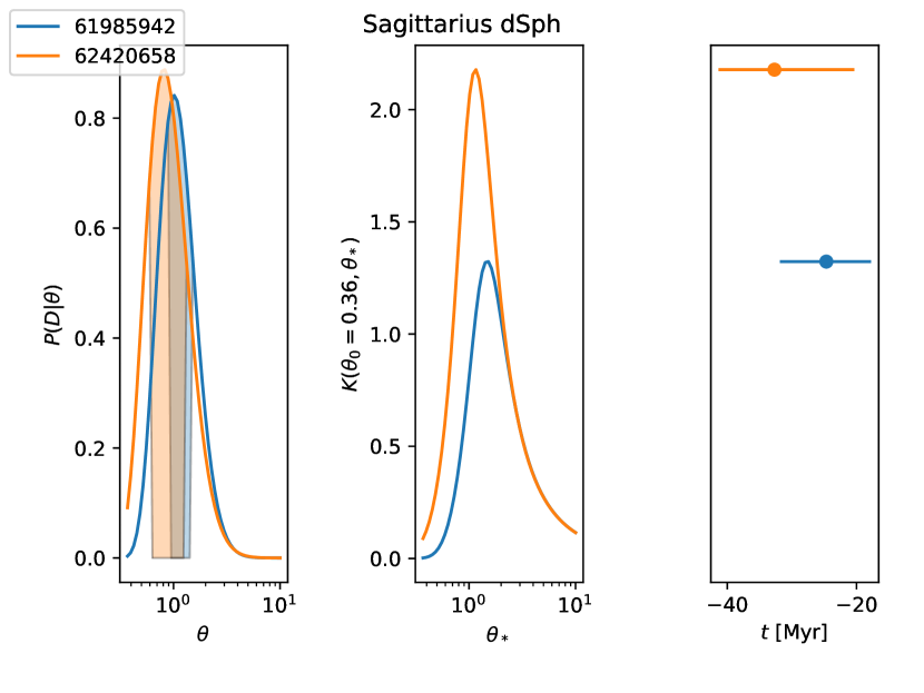
Figure 6: Stars compatible with having scattered with compact objects within Sagittarius dSph assuming Marchetti et al. (2019) distances. The legend shows the first 8 digits of Gaia DR2 star identification numbers. Left panel: Impact parameter likelihood. Filled regions are 68% confidence intervals. Central panel: Bayes factor for $\theta_{0}=0.36$ as a function of the upper prior threshold $\theta_{*}$. Right panel: Mean and 68% intervals for the intersection time (today corresponds to $t=0$ yr). The height of error bars is proportional to the respective maximum Bayes factor.

We first fix the prior lower threshold $\theta_{0}=0$ and search for scattering events within a given upper threshold $\theta_{*}$. Then we repeat the search for a few values of the lower prior threshold $\theta_{0}\leq 0.5$. This parameterise our belief that a scattering event is unlikely to take place in the innermost region of a given object, as it is the case if we look for interactions with the PBH CDM halo of a galaxy. We consider both Marchetti et al. (2019) and Anders et al. (2019) distance estimates. If $K>1$ then the star is compatible with having interacted with a given object.

In the case $\theta_{0}=0$ we do not find candidate scattering events (see however appendix A). As shown in figure 6, in the case of the Sagittarius dwarf spheroidal galaxy (Sagittarius dSph), we find two stars candidate to having scattered with compact objects within it when assuming Marchetti et al. (2019) distances for $\theta_{0}=0.36$, corresponding to the minor-to-major axis ratio for Sagittarius dSph given its ellipticity $\epsilon=0.64\pm 0.02$ (McConnachie, 2012). The Bayes factor peaks at values $\theta_{*}\sim 1$. Scattering times are about 20–40 Myr ago, excluding that these events are directly related to the fact that Sagittarius dSph may have crossed the Galactic disk 300–900 Myr ago (Antoja et al., 2018).

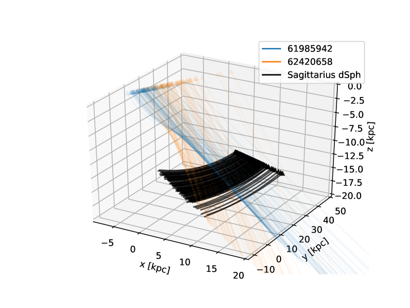
Figure 7: Orbits in Galactocentric Cartesian coordinates corresponding the same objects discussed in figure 6. Line density is proportional to the likelihood. Markers represent positions today.

Figure 7 shows 100 orbits randomly sampled from the respective likelihoods for objects discussed in figure 6. Distance uncertainties lead to large spreads in radial directions from the Sun. Trajectories beyond the scattering event are no longer reliable as they may be depend on a different potential, but that’s not a concern for our purposes.

In order to verify whether our results are compatible with the evolutionary status of our stars (i.e., whether their life time is enough to have crossed the very large distance from the original point), we derive their effective temperature (T_eff) and bolometric luminosity (L_bol) and compare with theoretical isochrones and evolutionary tracks. First, we obtain L_bol and T_eff using the Virtual Observatory SED Analyzer (VOSA, Bayo et al., 2008), by constructing a complete Spectral Energy Distribution (SED) taking advantage of different photometric repositories under Virtual Observatory (VO) protocols. Then, the basic properties are derived using atmospheric models by Kurucz (Castelli et al., 1997). We impose restrictions on the surface gravity ($\log g=2$) and metallicity ([Fe/H]=-0.5), based on the expectations about these candidates (they should be giant or subgiant stars with low metallicity, since Sagittarius dSph has [Fe/H]$=-0.40\pm 0.2$ dex (McConnachie, 2012)). In any case, SED fitting depends weakly on $\log g$ and our results are very similar if a larger degree of freedom is allowed. Thus, the T_eff range between 6000 and 4250 K, whereas the L_bol are bracketed between 620 and 2000 L_⊙. We have compared these values with PADOVA models (Marigo et al., 2017). Their position in a HR diagram clearly shows that they have masses in the range 3.5-6 M$\odot$ and they are either in the subgiant branch, close to the subgiant branch, or the Blue loop. Therefore, we can establish a lower limit for the age, about 100 Myr, fully compatible with our expectations.

Positive evidence is not confirmed when using Anders et al. (2019) distances. However, our result provides motivation to model a prior based on the actual three-dimensional DM distribution of Sagittarius dSph, a difficult issue that has to take into account strong tidal disruption.

More information about the sources discussed here is given in table 5.

5 Conclusions

We have defined a Bayesian framework to search for correlations between 1642 Gaia DR2 high-velocity star trajectories and those of 52 globular clusters (identified by Gaia DR2) and 35 Milky Way dwarf and nearby galaxies. We report 2 stars candidate to have scattered with compact objects within Sagittarius dSph roughly between 20 and 40 Myr ago when assuming distances estimated in Marchetti et al. (2019). Analysis of their evolutionary status leads to a lower bound of about 100 Myr for their age, fully compatible with the scattering time window. Results are not confirmed when assuming distances estimated in Anders et al. (2019).

These events may correspond to DM scattering, if the latter is composed by PBH able to accelerate significantly a star upon encounter. In principle the reported number of scattering events may be used to validate this hypothesis. However, given the statistically small sample considered here and uncertainties in PBH mass distribution we cannot put meaningful limits.

Marchetti et al. (2019) reported HVS candidates compatible with extragalactic origin. Their trajectory may also be explained if they scattered with DM bounded to a galaxy or GC. We repeated our search including their final HVS selection of 20 stars (with probability of being unbound larger than 80%), and we do not find evidence to support this hypothesis (furthermore several stars in their selection are contaminated by spurious radial velocities (Boubert et al., 2019)).

In defining the impact parameter based on the radius of a sphere centered around a given galaxy or GC, we have taken into account the necessity to analyze at once several heterogeneous objects. Studying the Bayes factor as a function of the marginal likelihood prior takes into account that the radius is only a proxy to the actual shape (e.g., Sagittarius dSph is characterized by a large ellipticity) or DM distribution (that can extend well beyond the optical size). Nevertheless, a follow-up analysis focused on Sagittarius dSph should define the impact parameter based on its actual shape and DM distribution, taking into account its time evolution.

Our results are highly dependent on the distance computation methodology. We find that Marchetti et al. (2019) distances are usually significantly larger than other catalogs for our stellar selection (see table 5). Distances estimated in Anders et al. (2019) are more in agreement with other computations (e.g., (Bailer-Jones et al., 2018) and Schönrich et al. (2019)) although results generally differ significantly for stars more distant than 3 kpc. This sensitivity on systematic effects (especially a global parallax zero-point difficult to model) calls for future confirmations based on more accurate parallax estimates.

Marchetti et al. (2018) showed that the majority of HVS expected to be detected by Gaia are fainter than the limiting magnitude to obtain radial velocities in DR2. Future data releases will include a larger number of stars with full phase-space information, together with improved astronomy and photometry. As our analysis shows, the understanding of systematic errors up to distances of around $10$ kpc is crucial for a robust search. More accurate data will also help to avoid spurious HVS identification possibly affecting our selection.

The fact that we only find candidate scattering events within Sagittarius dSph, relatively large and close, may be due to a selection effect that can be included in future analyses. In fact, if the events under consideration correspond to DM scattering, then we would expect to be able to detect a similar number of interactions also with other large galaxies such as LMC. It is important to repeat and possibly extend the search when future Gaia data releases will be available.

The main motivation of the present search is that HVS may be correlated to past scattering events with massive compact objects in dwarf galaxies. The same idea prompts another interesting prospect, i.e., using trajectories of HVS compatible with having extragalactic origin as a guide for discovery of faint dwarf galaxies, particularly relevant to extend catalogs of low surface brightness galaxies (Du et al., 2019) and for missions like the MESSIER surveyor (Valls-Gabaud, 2016).

Appendix A Alternative stellar selection

As an alternative to the stellar selection mentioned in section 2.1, here we consider 1747 stars that still satisfy cuts given in Marchetti et al. (2019), total heliocentric velocities $v-\sigma_{v}\gtrsim 500$ km/s and exclude possibly contaminated radial velocities (Boubert et al., 2019), but have an higher unbound probability threshold $P_{\rm ub}>0.9$. Most of the stars have negative parallax, an indicator of poor data quality due to the absence of further photometric and astrometric cuts.

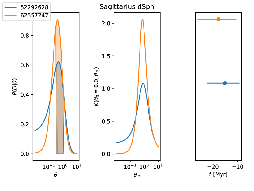
Figure 8: Same as figure 6, but for different stars. The Bayes factor in the central panel is computed setting a lower prior threshold $\theta_{0}=0$.

Assuming Marchetti et al. (2019) distances and setting a lower prior threshold $\theta_{0}=0$ for the computation of the Bayes factor, the same search described in section 4 brings to figure 8. Two stars are compatible with having scattered with compact objects in Sagitarius dSph 10–30 Myr ago. If we set $\theta_{0}=0.36$ as discussed in section 4, we find that the maximum Bayes factors increase to $K\sim 2,10$ for stars 52292628 and 62557247, respectively, and that a third star (62779130) has positive scattering evidence ($K\gtrsim 1$). We verified that all stars are compatible with being at least $\sim 80$ Myr old. (More information about these sources is given in table 5.)

However, results are not confirmed when we repeate the same search assuming Anders et al. (2019) distances. Furthermore, Anders et al. (2019) flags the aforementioned stars as possible spurious astrometry due to large renormalised unit-weight error (RUWE). Hence, in this case positive evidence for scattering events may be driven not only by distance estimate systematic errors, but also by poor astrometric fit.

Appendix B Galactocentric coordinates

Galactocentric coordinates are defined as a Cartesian right-handed system with the $x$-axis pointing from the position of the Sun projected on the Galactic midplane to the Galactic center, the $y$-axis roughly pointing towards Galactic longitude $\ell=90^{\circ}$ and the $z$-axis points roughly towards the North Galactic Pole (we define the Galactic plane to be the normal to the north pole of Galactic coordinates defined by Blaauw (1960)). The Galactic Center right-ascension and declination are taken to be $\alpha=17:45:37.224$ hr and $\delta=-28:56:10.23$ deg, respectively (Reid & Brunthaler, 2004). We assume the distance from the Sun to the Galactic Center to be $8.33\pm 0.35$ kpc (Gillessen et al., 2009) and its height above the Galactic midplane to be $27\pm 4$ pc (Chen et al., 2001). Galactocentric velocities are definied assuming a circular velocity of 220 km/s at solar radius (Bovy, 2015) and a Sun peculiar velocity with respect to the Galactic center $(V_{x},V_{y},V_{z})_{\sun}=(11.1\pm 0.74\pm 1,12.24\pm 0.47\pm 2,7.25\pm 0.37\pm 0.5)$ km/s with additional systematic errors $(1,2,0.5)$ km/s (Schönrich et al., 2010).

Appendix C Orbits data

Tales 2 and 3 list source identifiers for GC and galaxies used in the main analysis. Table 4 shows Sagittarius dSph phase-space data and size. Table 5 shows phase-space data and derived quantities for Gaia DR2 stars compatible with having scattered with compact objects within Sagittarius dSph when assuming Marchetti et al. (2019) distances.

GC, galaxy and star catalogs are available as ancillary files at https://arxiv.org/abs/1907.09298.

Table 2: Globular clusters identifiers.

NGC0104	NGC5272	NGC6218	NGC6388	NGC6656
NGC0288	NGC5286	NGC6254	NGC6397	NGC6681
NGC0362	NGC5466	NGC6266	NGC6440	NGC6752
NGC1851	NGC5897	NGC6273	NGC6453	NGC6779
NGC1904	NGC5904	NGC6284	NGC6522	NGC6809
NGC2298	NGC5986	NGC6287	NGC6535	NGC6838
NGC2808	NGC6093	NGC6293	NGC6541	NGC6864
NGC3201	NGC6121	NGC6304	NGC6544	NGC7078
NGC4372	NGC6144	NGC6341	NGC6626	NGC7089
NGC4833	NGC6171	NGC6352	NGC6637	NGC7099
NGC5139	NGC6205

Table 3: Nearby galaxy identifiers and detailed references (complementing those given in section 2.2) for position, size and other useful measurements. All systems are identified as dwarf galaxies, excluded Andromeda, Large Magellanic Cloud (LMC), Small Magellanic Cloud (SMC) and objects of ambiguous nature denoted by an asterisk (*).

*Draco II	Laevens et al. (2015b)
Grus 1	Koposov et al. (2015)
Horologium 1	Koposov et al. (2015); Bechtol et al. (2015)
Reticulum 2	Bechtol et al. (2015); Koposov et al. (2015)
Triangulum II	Laevens et al. (2015a)
Tucana III	Drlica-Wagner et al. (2015)
Andromeda	See section 2.2
Antlia II	See section 2.2
Bootes (I)	Dall’Ora et al. (2006); Martin et al. (2007); Martin et al. (2008b); Koposov et al. (2011); Grcevich & Putman (2009); Norris et al. (2010)
Bootes II	Walsh et al. (2008); Koch et al. (2009); Martin et al. (2008b); Grcevich & Putman (2009)
Canes Venatici (I)	Martin et al. (2008a); Simon & Geha (2007); Martin et al. (2008b); Grcevich & Putman (2009); Kirby et al. (2008, 2011)
Canes Venatici II	Greco et al. (2008); Simon & Geha (2007); Martin et al. (2008b); Grcevich & Putman (2009); Kirby et al. (2008, 2011)
Carina	Pietrzyński et al. (2009); Walker et al. (2009a); Irwin & Hatzidimitriou (1995); Walker et al. (2008); Grcevich & Putman (2009); Koch et al. (2006)
Coma Berenices	Belokurov et al. (2007); Simon & Geha (2007); Martin et al. (2008b); Grcevich & Putman (2009); Kirby et al. (2008, 2011)
Draco	Bonanos et al. (2004); Walker et al. (2007); Martin et al. (2008b); Wilkinson et al. (2004); Grcevich & Putman (2009); Kirby et al. (2011)
Eridanus 2	Koposov et al. (2015); Bechtol et al. (2015)
Fornax	Pietrzyński et al. (2009); Walker et al. (2009a); Irwin & Hatzidimitriou (1995); Walker et al. (2008, 2009b); Grcevich & Putman (2009); Kirby et al. (2011)
Hercules	Coleman et al. (2007); Adén et al. (2009); Martin et al. (2008b); Grcevich & Putman (2009); Kirby et al. (2008, 2011)
Hydra II	Martin et al. (2015); Kirby et al. (2015)
LMC	See section 2.2
Leo I	Bellazzini et al. (2004); Mateo et al. (2008); Irwin & Hatzidimitriou (1995); Grcevich & Putman (2009); Kirby et al. (2011)
Leo II	Bellazzini et al. (2005); Walker et al. (2007); Irwin & Hatzidimitriou (1995); Grcevich & Putman (2009); Kirby et al. (2011)
Leo IV	Moretti et al. (2009); Simon & Geha (2007); de Jong et al. (2010); Grcevich & Putman (2009); Kirby et al. (2008, 2011)
Leo V
SMC	See section 2.2
Sagittarius dSph	Ibata et al. (1994); Ibata et al. (1997); Mateo et al. (1998); Majewski et al. (2003); Monaco et al. (2004); Chou et al. (2007); Grcevich & Putman (2009); Peñarrubia et al. (2011)
Sculptor	Pietrzyński et al. (2008); Walker et al. (2009a); Irwin & Hatzidimitriou (1995); Walker et al. (2008); Carignan et al. (1998); Grcevich & Putman (2009); Kirby et al. (2009, 2011)
Segue (I)	Belokurov et al. (2007); Simon et al. (2011); Martin et al. (2008b); Grcevich & Putman (2009); Norris et al. (2010)
Segue II	Belokurov et al. (2009); Kirby et al. (2013)
Sextans (I)	Lee et al. (2009); Walker et al. (2009a); Irwin & Hatzidimitriou (1995); Walker et al. (2008); Grcevich & Putman (2009); Kirby et al. (2011)
Tucana 2	Koposov et al. (2015); Bechtol et al. (2015)
Ursa Major (I)	Okamoto et al. (2008); Simon & Geha (2007); Martin et al. (2008b); Grcevich & Putman (2009); Kirby et al. (2008, 2011)
Ursa Major II	Zucker et al. (2006); Simon & Geha (2007); Martin et al. (2008b); Grcevich & Putman (2009); Kirby et al. (2008, 2011)
Ursa Minor	Carrera et al. (2002); Walker et al. (2009c); Irwin & Hatzidimitriou (1995); Wilkinson et al. (2004); Grcevich & Putman (2009); Kirby et al. (2011)
Willman 1	Willman et al. (2006); Martin et al. (2007); Martin et al. (2008b); Grcevich & Putman (2009); Willman et al. (2011)

Table 4: Sagittarius dSph phase-space and size data. Rows correspond to right-ascension $\alpha$ and declination $\delta$ (ICRS at epoch J2000.0), distance modulus $\mu$, proper motions in right-ascension direction $\mu_{\alpha*}=\mu_{\alpha}\cos{\delta}$ and in declination direction $\mu_{\delta}$, radial velocity along the line-of-sight $V_{r}$ and half-light radius measured along the major axis $r_{h}$.

$\alpha$ [deg]	283.8313
$\delta$ [deg]	-30.4606
$\mu$	$17.13\pm 0.11$
$\mu_{\alpha*}$ [mas/yr]	$-2.736\pm 0.044$
$\mu_{\delta}$ [mas/yr]	$-1.357\pm 0.043$
$V_{r}$ [km/s]	$140\pm 2$
$r_{h}$ [arcmin]	$342\pm 12$

Table 5: HVS compatible with having scattered with compact objects within Sagittarius dSph. Columns correspond to Gaia DR2 source identifier, RA and declination, parallax, proper motion in RA direction $\mu_{\alpha*}=\mu_{\alpha*}\cos(\delta)$, proper motion in declination direction, proper motions correlation coefficient, radial velocity and heliocentric distance derived in Marchetti et al. (2019), heliocentric distance derived in Anders et al. (2019) and probability of being unbound from the Milky Way potential. The unbound probability relies on Marchetti et al. (2019) distances. Reference epoch for astrometric quantities is J2015.5. While here we report the full source identifier, in the main text we only refer to the first 8 digits. The first two stars are discussed in section 4, the others in appendix A

source	($\alpha$, $\delta$)	$\varpi$	$\mu_{\alpha*}$	$\mu_{\delta}$	$c_{\mu_{\alpha*}\mu_{\delta}}$	$V_{r}$	$d_{\rm Marchetti}$	$d_{\rm Anders}$	$P_{\rm ub}$
	[deg]	[mas]	[mas/yr]	[mas/yr]		[km/s]	[kpc]	[kpc]
6198594250104473728	(223.0436, -37.9298)	$0.10\pm 0.04$	$-21.14\pm 0.06$	$2.40\pm 0.05$	-0.12	$96.0\pm 1.3$	$9.4_{-2.0}^{+3.3}$	$5.8_{-1.3}^{+1.9}$	0.87
6242065813132837376	(241.4245, -24.0908)	$0.08\pm 0.04$	$-11.97\pm 0.07$	$2.71\pm 0.04$	$0.03$	$-60.5\pm 1.3$	$11.7_{-3.0}^{+4.8}$	$7.2_{-1.8}^{+1.8}$	0.54
5229262874909180928	(162.8655, -73.4932)	$-3.79\pm 1.14$	$-30.45\pm 2.16$	$38.96\pm 2.12$	$-0.08$	$51.9\pm 1.3$	$8.6_{-3.2}^{+4.8}$	$2.0_{-0.5}^{+1.8}$	0.97
6255724732546338688	(228.2981, -20.7720)	$-2.59\pm 0.73$	$-31.37\pm 1.42$	$10.88\pm 1.36$	$-0.12$	$-109.3\pm 0.8$	$8.6_{-3.6}^{+5.3}$	$2.3_{-0.8}^{+1.9}$	0.93
6277913053288720512	(214.1732, -20.3474)	$-2.02\pm 0.43$	$-40.19\pm 0.69$	$11.60\pm 0.54$	$-0.22$	$-39.7\pm 2.9$	$10.1_{-3.3}^{+5.5}$	$4.3_{-1.4}^{+2.5}$	1.00

References

- Adén et al. (2009) Adén D., et al., 2009, A&A, 506, 1147 (arXiv:0908.3489)
- Anders et al. (2019) Anders F., et al., 2019, A&A, 628, A94 (arXiv:1904.11302)
- Antoja et al. (2018) Antoja T., et al., 2018, Nature, 561, 360 (arXiv:1804.10196)
- Astropy Collaboration et al. (2013) Astropy Collaboration et al., 2013, A&A, 558, A33 (arXiv:1307.6212)
- Astropy Collaboration et al. (2018) Astropy Collaboration et al., 2018, AJ, 156, 123 (arXiv:1801.02634)
- Bailer-Jones et al. (2018) Bailer-Jones C. A. L., Rybizki J., Fouesneau M., Mantelet G., Andrae R., 2018, AJ, 156, 58 (arXiv:1804.10121)
- Bayo et al. (2008) Bayo A., Rodrigo C., Barrado Y Navascués D., Solano E., Gutiérrez R., Morales-Calderón M., Allard F., 2008, A&A, 492, 277 (arXiv:0808.0270)
- Bechtol et al. (2015) Bechtol K., et al., 2015, ApJ, 807, 50 (arXiv:1503.02584)
- Bellazzini et al. (2004) Bellazzini M., Gennari N., Ferraro F. R., Sollima A., 2004, MNRAS, 354, 708 (arXiv:astro-ph/0407444)
- Bellazzini et al. (2005) Bellazzini M., Gennari N., Ferraro F. R., 2005, MNRAS, 360, 185 (arXiv:astro-ph/0503418)
- Belokurov et al. (2007) Belokurov V., et al., 2007, ApJ, 654, 897 (arXiv:astro-ph/0608448)
- Belokurov et al. (2009) Belokurov V., et al., 2009, MNRAS, 397, 1748 (arXiv:0903.0818)
- Blaauw (1960) Blaauw A., 1960, MNRAS, 121, 164
- Bonaca et al. (2017) Bonaca A., Conroy C., Wetzel A., Hopkins P. F., Kereš D., 2017, ApJ, 845, 101 (arXiv:1704.05463)
- Bonanos et al. (2004) Bonanos A. Z., Stanek K. Z., Szentgyorgyi A. H., Sasselov D. D., Bakos G. Á., 2004, AJ, 127, 861 (arXiv:astro-ph/0310477)
- Boubert et al. (2019) Boubert D., et al., 2019, MNRAS, 486, 2618 (arXiv:1901.10460)
- Bovy (2015) Bovy J., 2015, ApJS, 216, 29 (arXiv:1412.3451)
- Butkevich & Lindegren (2014) Butkevich A. G., Lindegren L., 2014, A&A, 570, A62 (arXiv:1407.4664)
- Calcino et al. (2018) Calcino J., Garcia-Bellido J., Davis T. M., 2018, Mon. Not. Roy. Astron. Soc., 479, 2889 (arXiv:1803.09205)
- Carignan et al. (1998) Carignan C., Beaulieu S., Côté S., Demers S., Mateo M., 1998, AJ, 116, 1690 (arXiv:astro-ph/9807222)
- Carrera et al. (2002) Carrera R., Aparicio A., Martínez-Delgado D., Alonso-García J., 2002, AJ, 123, 3199 (arXiv:astro-ph/0203300)
- Castelli et al. (1997) Castelli F., Gratton R. G., Kurucz R. L., 1997, A&A, 318, 841
- Chen et al. (2001) Chen B., et al., 2001, ApJ, 553, 184
- Chou et al. (2007) Chou M.-Y., et al., 2007, ApJ, 670, 346 (arXiv:astro-ph/0605101)
- Clesse & García-Bellido (2017) Clesse S., García-Bellido J., 2017, Phys. Dark Univ., 15, 142 (arXiv:1603.05234)
- Coleman et al. (2007) Coleman M. G., et al., 2007, ApJ, 668, L43
- Dall’Ora et al. (2006) Dall’Ora M., et al., 2006, ApJ, 653, L109 (arXiv:astro-ph/0611285)
- Drlica-Wagner et al. (2015) Drlica-Wagner A., et al., 2015, ApJ, 813, 109 (arXiv:1508.03622)
- Du et al. (2019) Du W., Cheng C., Wu H., Zhu M., Wang Y., 2019, MNRAS, 483, 1754 (arXiv:1811.04569)
- ESA (1997) ESA ed. 1997, The HIPPARCOS and TYCHO catalogues. Astrometric and photometric star catalogues derived from the ESA HIPPARCOS Space Astrometry Mission ESA Special Publication Vol. 1200
- Einasto (1965) Einasto J., 1965, Trudy Astrofizicheskogo Instituta Alma-Ata, 5, 87
- Evans (1993) Evans N. W., 1993, MNRAS, 260, 191
- Evans (1994) Evans N. W., 1994, MNRAS, 267, 333
- Fritz et al. (2018) Fritz T. K., Battaglia G., Pawlowski M. S., Kallivayalil N., van der Marel R., Sohn S. T., Brook C., Besla G., 2018, A&A, 619, A103 (arXiv:1805.00908)
- Gaia Collaboration et al. (2016) Gaia Collaboration et al., 2016, A&A, 595, A1 (arXiv:1609.04153)
- Gaia Collaboration et al. (2018a) Gaia Collaboration et al., 2018a, A&A, 616, A1 (arXiv:1804.09365)
- Gaia Collaboration et al. (2018b) Gaia Collaboration et al., 2018b, A&A, 616, A12 (arXiv:1804.09381)
- García-Bellido (2017) García-Bellido J., 2017, J. Phys. Conf. Ser., 840, 012032 (arXiv:1702.08275)
- Gillessen et al. (2009) Gillessen S., Eisenhauer F., Trippe S., Alexand er T., Genzel R., Martins F., Ott T., 2009, ApJ, 692, 1075 (arXiv:0810.4674)
- Grcevich & Putman (2009) Grcevich J., Putman M. E., 2009, ApJ, 696, 385 (arXiv:0901.4975)
- Greco et al. (2008) Greco C., et al., 2008, ApJ, 675, L73 (arXiv:0712.2241)
- Hattori et al. (2018) Hattori K., Valluri M., Bell E. F., Roederer I. U., 2018, ApJ, 866, 121 (arXiv:1805.03194)
- Hernquist (1990) Hernquist L., 1990, ApJ, 356, 359
- Ibata et al. (1994) Ibata R. A., Gilmore G., Irwin M. J., 1994, Nature, 370, 194
- Ibata et al. (1997) Ibata R. A., Wyse R. F. G., Gilmore G., Irwin M. J., Suntzeff N. B., 1997, AJ, 113, 634 (arXiv:astro-ph/9612025)
- Irwin & Hatzidimitriou (1995) Irwin M., Hatzidimitriou D., 1995, MNRAS, 277, 1354
- Kirby et al. (2008) Kirby E. N., Simon J. D., Geha M., Guhathakurta P., Frebel A., 2008, ApJ, 685, L43 (arXiv:0807.1925)
- Kirby et al. (2009) Kirby E. N., Guhathakurta P., Bolte M., Sneden C., Geha M. C., 2009, ApJ, 705, 328 (arXiv:0909.3092)
- Kirby et al. (2011) Kirby E. N., Lanfranchi G. A., Simon J. D., Cohen J. G., Guhathakurta P., 2011, ApJ, 727, 78 (arXiv:1011.4937)
- Kirby et al. (2013) Kirby E. N., Boylan-Kolchin M., Cohen J. G., Geha M., Bullock J. S., Kaplinghat M., 2013, ApJ, 770, 16 (arXiv:1304.6080)
- Kirby et al. (2015) Kirby E. N., Simon J. D., Cohen J. G., 2015, ApJ, 810, 56 (arXiv:1506.01021)
- Koch et al. (2006) Koch A., Grebel E. K., Wyse R. F. G., Kleyna J. T., Wilkinson M. I., Harbeck D. R., Gilmore G. F., Evans N. W., 2006, AJ, 131, 895 (arXiv:astro-ph/0511087)
- Koch et al. (2009) Koch A., et al., 2009, ApJ, 690, 453 (arXiv:0809.0700)
- Koposov et al. (2011) Koposov S. E., et al., 2011, ApJ, 736, 146 (arXiv:1105.4102)
- Koposov et al. (2015) Koposov S. E., Belokurov V., Torrealba G., Evans N. W., 2015, ApJ, 805, 130 (arXiv:1503.02079)
- Laevens et al. (2015a) Laevens B. P. M., et al., 2015a, ApJ, 802, L18 (arXiv:1503.05554)
- Laevens et al. (2015b) Laevens B. P. M., et al., 2015b, ApJ, 813, 44 (arXiv:1507.07564)
- Lee et al. (2009) Lee M. G., Yuk I.-S., Park H. S., Harris J., Zaritsky D., 2009, ApJ, 703, 692 (arXiv:0907.5102)
- Lützgendorf et al. (2012) Lützgendorf N., et al., 2012, A&A, 543, A82 (arXiv:1205.4022)
- Majewski et al. (2003) Majewski S. R., Skrutskie M. F., Weinberg M. D., Ostheimer J. C., 2003, ApJ, 599, 1082 (arXiv:astro-ph/0304198)
- Marchetti et al. (2018) Marchetti T., Contigiani O., Rossi E. M., Albert J. G., Brown A. G. A., Sesana A., 2018, MNRAS, 476, 4697 (arXiv:1711.11397)
- Marchetti et al. (2019) Marchetti T., Rossi E. M., Brown A. G. A., 2019, MNRAS, 490, 157 (arXiv:1804.10607)
- Marigo et al. (2017) Marigo P., et al., 2017, ApJ, 835, 77 (arXiv:1701.08510)
- Martin et al. (2007) Martin N. F., Ibata R. A., Chapman S. C., Irwin M., Lewis G. F., 2007, MNRAS, 380, 281 (arXiv:0705.4622)
- Martin et al. (2008a) Martin N. F., et al., 2008a, ApJ, 672, L13 (arXiv:0709.3365)
- Martin et al. (2008b) Martin N. F., de Jong J. T. A., Rix H.-W., 2008b, ApJ, 684, 1075 (arXiv:0805.2945)
- Martin et al. (2015) Martin N. F., et al., 2015, ApJ, 804, L5 (arXiv:1503.06216)
- Mateo et al. (1998) Mateo M., Olszewski E. W., Morrison H. L., 1998, ApJ, 508, L55 (arXiv:astro-ph/9810015)
- Mateo et al. (2008) Mateo M., Olszewski E. W., Walker M. G., 2008, ApJ, 675, 201 (arXiv:0708.1327)
- McConnachie (2012) McConnachie A. W., 2012, AJ, 144, 4 (arXiv:1204.1562)
- Miyamoto & Nagai (1975) Miyamoto M., Nagai R., 1975, PASJ, 27, 533
- Monaco et al. (2004) Monaco L., Bellazzini M., Ferraro F. R., Pancino E., 2004, MNRAS, 353, 874 (arXiv:astro-ph/0406350)
- Moretti et al. (2009) Moretti M. I., et al., 2009, ApJ, 699, L125 (arXiv:0906.0700)
- Navarro et al. (1996) Navarro J. F., Frenk C. S., White S. D. M., 1996, Astrophys. J., 462, 563 (arXiv:astro-ph/9508025)
- Newton et al. (2018) Newton O., Cautun M., Jenkins A., Frenk C. S., Helly J., 2018, Mon. Not. Roy. Astron. Soc., 479, 2853 (arXiv:1708.04247)
- Norris et al. (2010) Norris J. E., Wyse R. F. G., Gilmore G., Yong D., Frebel A., Wilkinson M. I., Belokurov V., Zucker D. B., 2010, ApJ, 723, 1632 (arXiv:1008.0137)
- Okamoto et al. (2008) Okamoto S., Arimoto N., Yamada Y., Onodera M., 2008, A&A, 487, 103 (arXiv:0804.2976)
- Peñarrubia et al. (2011) Peñarrubia J., et al., 2011, ApJ, 727, L2 (arXiv:1011.6206)
- Pietrzyński et al. (2008) Pietrzyński G., et al., 2008, AJ, 135, 1993 (arXiv:0804.0347)
- Pietrzyński et al. (2009) Pietrzyński G., Górski M., Gieren W., Ivanov V. D., Bresolin F., Kudritzki R.-P., 2009, AJ, 138, 459 (arXiv:0906.0082)
- Price-Whelan (2017) Price-Whelan A. M., 2017, The Journal of Open Source Software, 2, 388
- Reid & Brunthaler (2004) Reid M. J., Brunthaler A., 2004, ApJ, 616, 872 (arXiv:astro-ph/0408107)
- Schönrich (2012) Schönrich R., 2012, MNRAS, 427, 274 (arXiv:1207.3079)
- Schönrich et al. (2010) Schönrich R., Binney J., Dehnen W., 2010, MNRAS, 403, 1829 (arXiv:0912.3693)
- Schönrich et al. (2019) Schönrich R., McMillan P., Eyer L., 2019, MNRAS, 487, 3568 (arXiv:1902.02355)
- Simon & Geha (2007) Simon J. D., Geha M., 2007, ApJ, 670, 313 (arXiv:0706.0516)
- Simon et al. (2011) Simon J. D., et al., 2011, ApJ, 733, 46 (arXiv:1007.4198)
- Simon et al. (2019) Simon J., et al., 2019, BAAS, 51, 409 (arXiv:1903.04743)
- Taylor (2005) Taylor M. B., 2005, in Shopbell P., Britton M., Ebert R., eds, Astronomical Society of the Pacific Conference Series Vol. 347, Astronomical Data Analysis Software and Systems XIV. p. 29
- Taylor (2006) Taylor M. B., 2006, in Gabriel C., Arviset C., Ponz D., Enrique S., eds, Astronomical Society of the Pacific Conference Series Vol. 351, Astronomical Data Analysis Software and Systems XV. p. 666
- Torrealba et al. (2019) Torrealba G., et al., 2019, MNRAS, 488, 2743 (arXiv:1811.04082)
- Valls-Gabaud (2016) Valls-Gabaud D., 2016. Cambridge University Press, pp 199–201, doi:10.1017/S1743921316011388
- Walker et al. (2007) Walker M. G., Mateo M., Olszewski E. W., Gnedin O. Y., Wang X., Sen B., Woodroofe M., 2007, ApJ, 667, L53 (arXiv:0708.0010)
- Walker et al. (2008) Walker M. G., Mateo M., Olszewski E. W., 2008, ApJ, 688, L75 (arXiv:0810.1511)
- Walker et al. (2009a) Walker M. G., Mateo M., Olszewski E. W., 2009a, AJ, 137, 3100 (arXiv:0811.0118)
- Walker et al. (2009b) Walker M. G., Belokurov V., Evans N. W., Irwin M. J., Mateo M., Olszewski E. W., Gilmore G., 2009b, ApJ, 694, L144 (arXiv:0902.3003)
- Walker et al. (2009c) Walker M. G., Mateo M., Olszewski E. W., Peñarrubia J., Evans N. W., Gilmore G., 2009c, ApJ, 704, 1274 (arXiv:0906.0341)
- Walsh et al. (2008) Walsh S. M., Willman B., Sand D., Harris J., Seth A., Zaritsky D., Jerjen H., 2008, ApJ, 688, 245 (arXiv:0712.3054)
- Wenger et al. (2000) Wenger M., et al., 2000, Astron. Astrophys. Suppl. Ser., 143, 9 (arXiv:astro-ph/0002110)
- Wilkinson et al. (2004) Wilkinson M. I., Kleyna J. T., Evans N. W., Gilmore G. F., Irwin M. J., Grebel E. K., 2004, ApJ, 611, L21 (arXiv:astro-ph/0406520)
- Willman et al. (2006) Willman B., et al., 2006, arXiv e-prints, pp astro–ph/0603486 (arXiv:astro-ph/0603486)
- Willman et al. (2011) Willman B., Geha M., Strader J., Strigari L. E., Simon J. D., Kirby E., Ho N., Warres A., 2011, AJ, 142, 128 (arXiv:1007.3499)
- Zucker et al. (2006) Zucker D. B., et al., 2006, ApJ, 650, L41 (arXiv:astro-ph/0606633)
- de Jong et al. (2010) de Jong J. T. A., Martin N. F., Rix H.-W., Smith K. W., Jin S., Macciò A. V., 2010, ApJ, 710, 1664 (arXiv:0912.3251)
- van der Marel et al. (2012) van der Marel R. P., Fardal M., Besla G., Beaton R. L., Sohn S. T., Anderson J., Brown T., Guhathakurta P., 2012, ApJ, 753, 8 (arXiv:1205.6864)