Measure the temperature of the spin via weak measurement

Abstract

In this study, we give a new proposal to measure the temperature of the spin in a sample in magnetic resonance force microscopy system by using postselected weak measurement, and investigate the fisher information to estimate the precision of our scheme. We showed that in high temperature regime the temperature of the spin can be measured via weak measurement technique with proper postselection and our scheme able to increase the precision of temperature estimation.

I Introduction

Measurement is a basic concept in physics and any information of the system can be obtained from the measurement. Unlike the classical measurement, in most of the quantum measurement processes the information of the system only can be obtained or estimated by using indirect measurements. Using quantum measurement terminology, in a quantum measurement process, there have an interaction between measuring device (probe) and measured system, and for guarantee the measurement precision the interaction time must be very short so that the system and the probe itself doesn’t effect the results of measurements. In mathematics, these requirements of quantum measurement can be expressed by von Newmann Hamiltonian $H=g\hat{A}\otimes\hat{P}$Neumann . Here, $\hat{A}$ is the operator of measured system we want to measure, $\hat{P}$ the canonical momentum of measuring device, and $g$ represent the measuring strength. If the interaction strength between the system and the probe is strong, i.e. $g\gg 1$, we can get the information of the system by single trial with very small error, the Stern-Gerlah experiment is a typical example. In contrast, if the interaction strength between probe and system is very small, i.e. $g\ll 1$, there have still interference between different eigenvalues of the system observable we want to measure, and after single trial we can not obtain the information of the system precisely.

However, the weak measurement, as a generalized von Neumann quantum measurement theory, was proposed by Aharonov, Albert, and Vaidman in 1988 opens a new route to measure the system information in weak coupling measurement problemsAharonov(1988) . In weak measurement technique, the coupling between the pointer and the measured systems is sufficiently weak,and the obtained information by single trial is trivial, but using its inherent feature one can get enough information as precisely as possibleTollaksen(2010) . One of the distinguished properties of weak measurement compared with strong measurement is that its induced weak value of the observable on the measured system can be beyond the usual range of the eigenvalues of that observableqparadox(2005) . The feature of weak value usually referred to as an amplification effect for weak signals rather than a conventional quantum measurement and used to amplify many weak but useful information in physical systemsDressel(2014) ; Nori ; Shikano(2010) . So far, the weak measurement technique has been applied in different fields to investigate very tiny effects, such as beam deflectionPfeifer(2011) ; Hosten2008 ; Hogan(2011) ; Zhou(2013) ; Starling(2009) ; Dixon(2009) , frequency shiftsStarling(2010)-1 , phase shiftsStarling(2010) , angular shiftsMagana(2013) ; Bertulio(2014) , velocity shiftsviza(2013) , and even temperature shiftEgan(2012) . Furthermore, it has been applied to solve some fundamentals of quantum physics such as quantum paradoxes(Hardy’s paradoxAharonov(2002) ; Lundeen(2009) ; Yokota(2009) and the three-box paradoxResch(2004) ), quantum correlation and quantum dynamicsAharonov(2005) ; Aharonov(2008) ; Holger(2013) ; Shikano(2012) ; Aharonov(2011) ; Shikano(2011) , quantum state tomographyLundeen(2012) ; Braveman(2013) ; Kocsis(2011) ; Malik(2014) ; Salvail(2013) ; Lundeen(2011) , violation of the generalized Leggett-Garg inequalitiesPalacios ; Suzuki(2012) ; Emary(2014) ; Goggin(2011) ; Groen(2013) ; Dressel(2011) and the violation of the initial Heisenberg measurement-disturbance relationshipLee(2012) ; Eda(2014) ,etc.

We know that temperature is a basic concept in thermodynamics and most of the properties of a matter is directly related with its temperature. According to the thermodynamics the temperature is an intensive quantity and independent to sample’s volume and mass. Thus, it is possible to measure the temperature of nanoscale objects which inserted in large sample. The motion of nanoscale objects obey the quantum mechanics and with the recent progress to manipulation of individual quantum systems, it has been possible to temperature readings with nanometric spatial resolutionNeu ; Kubo ; Toyli . Quantum thermometery also applied to precisely estimate the temperature of fermonicHauck ; Haupt and bosonicWhite ; Braun hot reservoirs, micromechanical resonatorsBruelli2 ; Brunelli ; Higgins and nuclear spinsRaitz . The nanoscale system is too fragile and measuring the temperature of such systems requires that the measurement process should not disturb them to much while keeping the high measurement precision. Furthermore, as investigated in previous studiesDressel(2014) , the weak measurement almost doesn’t destroy the measured system and can get the desired system information via statistical techniques with high precision. Thus,here raising an intriguing question as to whether one can measure the temperature of nanoscale objects by using postselected weak measurement technique. In recent studyPati(2019) , they investigated the method to measure the temperature of a bath using the postselected weak measurement scheme with a finite dimensional probe, and anticipated more applications of post weak measurement method in thermometry.

In this paper, motivated by the previous studyPati(2019) , we investigate to measure the temperature of nanoscale system(spin) which inserted in large thermal reservoir by using postselected weak measurement. We assume that there have a weak interaction between spin and cantilever in magnetic resonance force microscopy(MRFM) systemBerman . We show that the temperature of the spin which stayed in hot reservoir with termpreature $T$, can be measured by postselected weak measurement technique with proper postselected states of the spin, and the weak value can be read out from optical experimental processes. In temperature estimation process the fluctuation always exists due to the indirect measurement, but the quantum estimation theory provides the tool to evaluate lower bounds to the amount of fluctuations for a given measurement. To investigate the precision of our method, we evaluate the fisher information(FI) for the estimation of temperature via postselected weak measurement. We found that in high temperature regime the FI is more larger than unity with proper postselected states of the spin, and this enable us to show that postselected meak measurement method is indeed cane be used in temperature estimation process in MRFM system with high presicion.

The rest of the paper is organized as follows. In Sec. II, we give the setup for our system. In Sec. III, we give the details how to measure the temperature of a spin via postselected weak measurement. In Sec. IV, we investigate the Fisher information to investigate the precision of our scheme.We give a conclusion to our paper in Sec. V.

II Model setup

As illustrated in Fig.1, two ends of a cantilever used in MRFM is fixed and a small ferromagnetic particle is attached at the middle of the cantileverBerman . The force produced by a single spin on the ferromagnetic particle effects the parameters of the mechanical vibrations of the cantilever. There have a external permanent magnetic field $B_{ext}$ directed in the $z$ direction exerts on the spin and a ferromagnetic particle attached on the middle of the cantilever also exerts a gradient dipole magnetic field produced by the ferromagnetic particle on the spin $\partial B_{d}$/$\partial z$ with $B_{d}=\frac{2}{3}\mu_{0}M_{0}(\frac{R_{0}}{R_{0}+d+z})^{3},$ where $\mu_{0}$ is the permeability of the free space, $d$ is the distance between the bottom of the ferromagnetic particle and the spin is initially at equilibrium position($z=0$), $R_{0}$ and $M_{0}$ are the radius and magnetization of the ferromagnetic particle,respectively. The spin also exposed to the transversal frequency modulated rf magnetic field $\vec{B}_{1}(t)=B_{1}\left(\cos(\omega t+\phi(t)),\sin(\omega t+\phi(t)),0\right)$ in $x-y$ plane. The motion of the cantilever with ferromagnetic particle can be modeled as a simple harmonic oscillator with effective mass $m$ and frequency $\omega_{c}$. we can express the oscillation position $z$ of the cantilever with creation and annihilation operators $\hat{a}$ and $\hat{a}^{\dagger}$ by $\hat{z}=\sigma(\hat{a}+\hat{a}^{\dagger})$, with $\sigma=\sqrt{\text{$\hbar$}/2m\omega_{c}}$. In the rotating system coordinates(RSC) the Hamiltonian of this system can be written asBerman

$$H =\hbar\omega_{c}\hat{a}^{\dagger}\hat{a}+\hbar\omega_{z}\hat{S}_{z}+\hbar\omega_{R}\hat{S}_{x}-\hbar g\hat{S}_{z}\otimes\hat{z}.$$ (1)

Here, $\omega_{R}=\gamma B_{1}$, $\omega_{z}=\gamma B_{0}-\omega-\frac{d\phi}{dt}$ , $g=\gamma\frac{\partial B_{d}}{\partial z}$, $\gamma$ is the gyromagnetic ratio and $B_{0}=B_{ext}+B_{d}^{(0)}$ is the total magnetic field on the spin when $z=0$ in $z$ direction, and the gradient of the dipole field $\partial B_{d}$/$\partial z$ is taken at the spin location when $z=0$. $\hat{S}_{z,x}$are defined by Pauli operators $\hat{S}_{x}\rightarrow\frac{1}{2}\hat{\sigma}_{x}$ and $\hat{S}_{z}\rightarrow\frac{1}{2}\hat{\sigma}_{z}$, respectively. As we can see, our coupling system Hamiltonian consists of three parts(see Eq.1); first term represents the motion of cantilever, middle two terms describes the spin system and we denote with $H_{s}$, and the final term describes the interaction of spin and cantilever, and we denote it with $H_{int}$. According to the technique of MRFM, if the frequency of the spin oscillations matches the resonance frequency of the cantilever vibrations, the spin force will amplify the vibrations of the cantilever and its motion can be detected by optical methodsBerman . In this study, we will focus on to measure the temperature of the single spin which stayed in reservoir with temperature $T$ in MRFM system. Hereafter, in this paper we use the unit $\hbar=1$.

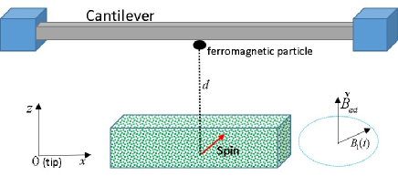
Figure 1: (Color online) The setup of our scheme. A spin and the cantilever are coupled with each other by a tiny ferromagnetic particle attached to the middle of the cantilever. $d$ is the distance between the bottom of the ferromagnetic particle and the spin at equilibrium position, $z=0$.

III Measure the temperature of the spin

As given in Eq.(1), the interaction Hamiltonian between the system(spin) and pointer(cantilever) is given by the standard von Neumman Hamiltonianqparadox(2005)

$$H_{ini}=-g\hat{S}_{z}\otimes\hat{z}$$ (2)

Here, $g$ is a coupling coefficient between spin and cantilever, and its value depends on gyromagnetic ratio $\gamma$ and the gradient magnetic field at the spin position produced by ferromagnetic particle. $\hat{z}=\int z|z\rangle\langle z|dz$ is the position operator,while the conjugate momentum operator is $\hat{p}=\int p|p\rangle\langle p|dp$ where $[\hat{x},\hat{p}]=i\text{$\hat{I}$}$. We consider the spin as system and cantilever as measuring device(pointer) to measure the temperature of the spin. We assume that initially the system (spin) is in a heat bath with temperature $T$, and reached the thermal equilibrium state $\text{$\rho$}_{s}=e^{-\beta H_{s}}/Tr(e^{-\beta H_{s}})$. Here $\beta=1/k_{B}T$ , $k_{B}$ is Boltzmann constant and it taken as unity hereafter. We assume that the initial state of measuring device and system are prepared as $\phi(z)=\langle z|\phi\rangle$ and $\rho(0)=\rho_{s}$, respectively. Then, under the action of unitary evolution operator $U(t)=\exp(-i\int_{0}^{t}H_{ini}d\tau)$, the initial state of total system $\rho(0)=\rho_{s}\otimes|\phi\rangle\langle\phi|$ will be evolved to

$$\text{$\rho(t)=U^{\dagger}(t)\rho(0)U(t)$}.$$ (3)

This is the state of the total system after interaction, but we only interested on final state of measuring device(cantilever) which contains system information. If we assume that the interaction strength $g$ is very small , then it is enough to consider the expansion of unitary operator up to its first order, and Eq.(3) becomes as

$$\rho(t)\approx\rho_{s}\otimes|\phi\rangle\langle\phi|+igt\left[\hat{S}_{z}\otimes\hat{z},\rho_{s}\otimes|\phi\rangle\langle\phi|\right].$$ (4)

According the standard terminology and procedure of weak measurement theory, if we choose the state $|\psi_{f}\rangle$ as the final state of the spin, and project it onto the total system state, Eq.(4), it gives the unnormalized final state of measuring device as

$$\phi(t)\approx\langle\psi_{f}|\rho_{s}|\psi_{f}\rangle e^{igt\text{$\hat{S}$}_{w}\hat{z}}|\phi\rangle\langle\phi|e^{-igt\hat{S}_{w}\hat{z}}.$$ (5)

Here,

$$S_{w} \frac{\langle\psi_{f}|\hat{S}_{z}\rho_{s}|\psi_{f}\rangle}{\langle\psi_{f}|\rho_{s}|\psi_{f}\rangle}$$= (6)

is the weak value of spin $z$ component and it related to the initial state of the spin which reached thermal equilibrium with a heat bath with temperature $T$. As can see from Eq.(5) and Eq.(6), we can deduce the spin temperature by properly choosing the final state$|\psi_{f}\rangle$. However, we have to note that $|\psi_{f}\rangle$ cannot be eigenstate of operator $\hat{S}_{z}$, otherwise the temperature will not related to the weak value and our scheme will lose its validity to measure the temperature of the spin.

To read the temperature of the spin system, next we will study the property of weak value of spin operator $\hat{S}_{z}$ by assuming that it in the hot bath with high temperature, i.e. $\beta\ll 1$. Furthermore, we assume that the eigenvalues of $\hat{S}_{x}$ and $\hat{S}_{y}$ are $\epsilon_{m}$and $\varepsilon_{m}$, and the corresponding eigenstates are $|\psi_{m}\rangle$ and $|\varphi_{m}\rangle$, i.e.,$\hat{S}_{x}|\psi_{m}\rangle=\epsilon_{m}|\psi_{m}\rangle$ and $\hat{S}_{z}|\varphi_{m}\rangle=\varepsilon_{m}|\varphi_{m}\rangle$, respectively. Then, the weak value of the spin $z$ component can be rewritten as

$$S_{w} =\frac{\langle\psi_{f}|\hat{S}_{z}e^{-\beta H_{s}}|\psi_{f}\rangle}{\langle\psi_{f}|e^{-i\beta H_{s}}|\psi_{f}\rangle}$$

$$=\frac{\sum_{n,m}e^{-\beta(\omega_{z}\varepsilon_{n}+\omega_{R}\epsilon_{m})}\langle\psi_{n}|\phi_{m}\rangle\langle\psi_{f}|\text{$\hat{S}_{z}$}|\psi_{n}\rangle\langle\phi_{m}|\psi_{f}\rangle}{\sum_{n,m}e^{-\beta(\omega_{z}\varepsilon_{n}+\omega_{R}\epsilon_{m})}\langle\psi_{n}|\phi_{m}\rangle\langle\psi_{f}|\psi_{n}\rangle\langle\phi_{m}|\psi_{f}\rangle}$$

$$=\frac{\langle\psi_{f}|\hat{S_{z}}|\psi_{f}\rangle-\beta\langle\psi_{f}|\hat{S_{z}}\hat{H}_{s}|\psi_{f}\rangle}{1-\beta\langle\psi_{f}|\hat{H}_{s}|\psi_{f}\rangle}.$$ (7)

During the derivation of Eq.(7), we use $e^{\pm x}\approx 1\pm x$, $(x\ll 1)$, and completeness of the basis $|\psi_{m}\rangle,\text{$|\varphi_{m}\rangle,$i.e. $\text{$\sum_{m}|\psi_{m}\rangle\langle\psi_{m}|=\sum_{m}|\varphi_{m}\rangle\langle\varphi_{m}|=1.$}$}$Since $(1-x)^{-1}\approx 1-x,(x\ll 1)$, we can rewrite the Eq.(7) as below

$$S_{w}=\left[\langle\psi_{f}|\hat{S_{z}}|\psi_{f}\rangle-\beta\langle\psi_{f}|\hat{S_{z}}\hat{H}_{s}|\psi_{f}\rangle\right]\left(1-\beta\langle\psi_{f}|\hat{H}_{s}|\psi_{f}\rangle\right).$$ (8)

From this relation, we can express the temperature parameter $\beta$ by using the weak value $S_{w}$ as

$$\beta=\frac{S_{w}-\langle\hat{S}_{z}\rangle}{Conv(S_{z},H_{s})-\langle\psi_{f}|\hat{S}_{z}\hat{H_{s}}|\psi_{f}\rangle},$$ (9)

where $Conv(S_{z},H_{s})=\langle\hat{S}_{z}\rangle\langle\psi_{f}|\hat{H}_{s}|\psi_{f}\rangle$ and $\langle\hat{S}_{z}\rangle=\langle\psi_{f}|\hat{S}_{z}|\psi_{f}\rangle$, respectively. From Eq.(9) we can see that since the value of $\langle\hat{S}_{z}\rangle$ and $Conv(S_{z},H_{s})$ can be find by using postselection $|\psi_{f}\rangle$, if we can find the value of $S_{w}$, then the temperature of the spin can be estimated very easily. For example, if we take $|\psi_{f}\rangle=\frac{1}{\sqrt{2}}(|\psi_{1}\rangle+|\psi_{2}\rangle)$, then Eq.(9) reduced to

$$\beta=\frac{2(1-2S_{w})}{\omega_{R}+3\omega_{z}}.$$ (10)

From the above theoretical results we can deduce that the estimation of spin in MRFM system depends on the postselected weak value. Thus, in the remaining part of this section we will discuss the possibility to find the weak value of our scheme. We can assume that the motion of the cantilever can be described by simple harmonic oscillator, and its initial state can be written as

$$\phi_{0}\left(z\right)=\langle z|0\rangle=\left(\frac{1}{2\pi\sigma^{2}}\right)^{\frac{1}{4}}\exp\left(-\frac{z^{2}}{4\sigma^{2}}\right)$$ (11)

where $\sigma$ is the width of the oscillation beam. The normalized final state of the cantilever after postselection, i.g. Eq.(5), can be written as

$$|\phi_{f}\rangle=\text{$\kappa$}[|0\rangle+ig_{0}S_{w}|1\rangle],$$ (12)

where $g_{0}=gt\sigma$, $\kappa=(1+g_{0}^{2}|S_{w}|^{2})^{-\frac{1}{2}}$ and we the $\phi_{0}(z)=\langle z|0\rangle$ and $\phi_{1}(z)=\langle z|1\rangle$ represent the ground and first excited states of catilever, respectively. The expectation values the position and momentum operators under the final state of the catilever $|\phi_{f}\rangle$ can be calculated as

$$\langle z\rangle =-2\sigma g_{0}\kappa^{2}\Im S_{w}$$ (13)

and

$$\langle p\rangle =\frac{\kappa^{2}g_{0}}{\sigma}\Re(S_{w})$$ (14)

respectively. According to the results of recent studiesYutaka(2014) ; Lundeen(2019) , we can measure the real and imaginary parts of the weak values with optical experiments. Thus, in our scheme the temperature of spin can be measured in the Lab with proper optical experimental setups.

IV Precision of our scheme

Fisher information is the maximum amount of information about the parameter that we can estimate from the system. For a pure quantum state $|\phi\rangle$, the quantum fisher information estimating the parameter $\beta$ is

$$F(\beta)=4[\langle\partial_{\beta}\text{$\phi$}|\partial_{\beta}\phi\rangle-|\langle\phi|\partial_{\beta}\phi\rangle|^{2}],$$ (15)

where the state $|\phi\rangle$is the normalized final state of the cantilever, i.e. Eq.(12). The variance of unknown parameter $\triangle\beta$ is bounded by the Cramér-Rao bound

$$Var\left(\beta\right)\geq\frac{1}{NF(\beta)},$$ (16)

where $N$ is the number of measurements. From this definition of variance of parameter $\beta$, we can see that the Fisher information set the minimal possible estimate for parameter $\beta$, while higher Fisher information means a better estimation. As the variance of $\beta$ is inverse proportional to the measurement time, we consider $N=1$ throughout this paper.

We investigate the variation of quantum Fisher information for different postselected states $|\psi_{f}\rangle=\cos\frac{\theta}{2}|\uparrow\rangle+e^{i\varphi}\sin\frac{\theta}{2}|\downarrow\rangle$ where $\theta\in[0,\pi],\varphi\in[0,2\pi)$, and $|\uparrow\rangle$ and $|\downarrow\rangle$ are eigenvector of the spin operator $\hat{S}_{z}$ with corresponding eigenvalues $+\frac{1}{2}$ and $-\frac{1}{2}$, respectively. Our numerical results in Fig.2 and Fig.3 show that the quantum Fisher information is higher in high temperature regime, and phase of postselected state also can effect of the precision of our scheme. However, as we mentioned in this section, when the postselected state is an eigenstate of the spin operator $\hat{S}_{z}$, the Fisher information become zero and our scheme lose its validity of measure the temperature of the spin.

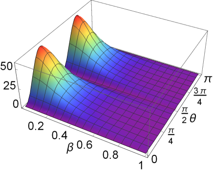
Figure 2: (Color online) Quantum fisher information for parameter estimation $\beta.$ Here, we take $\phi=0,g_{0}=10^{-8},\omega_{z}=4.8\times 10^{6}Hz$ , $\omega_{R}=3\times 10^{9}Hz$.

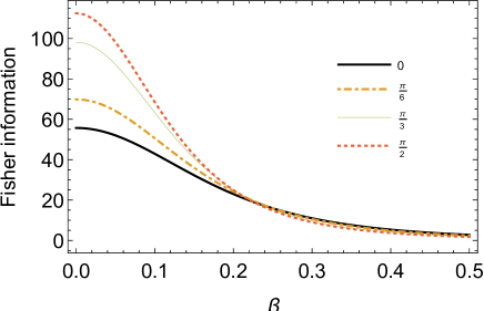
Figure 3: (Color online) Quantum fisher information for parameter estimation $\beta$ with different phase of postselected states. Here $\theta=\frac{\pi}{4}$ and other parameters are the same with Fig.2.

V Conclusion

In this study, we have proposed a new scheme to measure the temperature of spin which put it in thermal bath with temperature $T$ by using postselected weak measurement method. We find that in high temperature regime, the precision of our proposal is high enough and can be controlled by adjusting the parameters of postselected states of the spin. Furthermore, in Ref.Brun , the authors studied that quantum Fisher information is higher in postselected rather than non-postselected weak measurement.Thus, even though we only consider the high temperature regime, but in our scheme if someone use the postselected measurement, it will show its good performance in low temperature regime rather than non-postselected measurement schemes.

- (1) von Neumann J 1955 Mathematical Foundations of Quantum Mechanics (Princeton: Princeton University Press); published in German, 1932
- (2) Y. Aharonov, D.Z. Albert, and L. Vaidman, Phys. Rev. Lett. 60, 1351 (1988).
- (3) J. Tollaksen et al., New J. Phys.12, 013023(2010).
- (4) Y. Aharonov, D. Rohrlich, Quantum Paradoxes- Quantum Theory for the Perplexed (WILEY-VCH Verlag GmbH & Co. KGaA).
- (5) A. Hosoya and Y. Shikano, J. Phys. A 43, 385307 (2010).
- (6) A. G. Kofman, S. Ashhab, and F. Nori, Phys. Rep. 520, 43 (2012).
- (7) J. Dressel, M. Malik, F. M. Miatto, A. N. Jordan, and R. W. Boyd, Rev. Mod. Phys. 86, 307 (2014).
- (8) O. Hosten and P. Kwiat, Science 319, 787 (2008).
- (9) P. B. Dixon, D. J. Starling, A. N. Jordan, and J. C. Howell, Phys. Rev. Lett. 102, 173601 (2009).
- (10) D. J. Starling, P. B. Dixon, A. N. Jordan, and J. C. Howell, Phys. Rev. A 80, 041803(R) (2009).
- (11) J. M. Hogan, J. Hammer, S.-W. Chiow, S. Dickerson, D. M. S. Johnson, T. Kovachy, A. Sugarbaker, and M. A. Kasevich, Opt. Lett. 38, 1698 (2011).
- (12) M. Pfeifer, and P.Fischer, Opt.Exp 19, 16508 (2011).
- (13) L. Zhou, Y. Turek, C. P. Sun, and F. Nori, Phys. Rev. A 88, 053815 (2013).
- (14) D. J. Starling, P. B. Dixon, A. N. Jordan, and J. C. Howell, Phys. Rev. A 82, 063822 (2010).
- (15) D. J. Starling, P. B. Dixon, N. S. Williams, A. N. Jordan, and J. C. Howell, Phys. Rev. A 82, 011802(R) (2010).
- (16) O. S. Magaña-Loaiza, M. Mirhosseini, B. Rodenburg, and R. W. Boyd, Phys. Rev. Lett. 112, 200401 (2014).
- (17) B. de Lima Bernardo, S. Azevedo, and A. Rosas. Phys. Lett. A 378, 2029 (2014).
- (18) G. I. Viza, J. Martinez-Rincon, G. A. Howland, H. Frosting, I. Shromroni, B. Dayan, and J. C. Howell, Opt. Lett. 38, 2949 (2013).
- (19) P. Egan and J. A. Stone, Opt. Lett. 37, 4991 (2012).
- (20) Y. Aharonov, A. Botero, S. Popescu, B. Reznik, and J. Tollaksen, Phys. Lett. A 301, 130 (2002).
- (21) J. S. Lundeen and A. M. Steinberg, Phys. Rev. Lett. 102, 020404 (2009).
- (22) K. Yokota, T. Yamamoto, M. Koashi, and N. Imoto, New J. Phys. 11, 033011 (2009).
- (23) K. J. Resch, J. S. Lundeen, and A. M. Steinberg, Phys. Lett. A 324, 125 (2004).
- (24) Y. Aharonov and D. Rohrlich, Quantum Paradoxes: Quantum Theory for the Perplexed (Wiley-VCH, Weinheim, 2005).
- (25) Y. Aharonov and L. Vaidman, in Time in Quantum Mechanics, Vol. 1, edited by J. G. Muga, R. Sala Mayato, and I. L. Egusquiza (Springer, Berlin Heidelberg, 2008), p. 399.
- (26) Y. Aharonov and J. Tollaksen, in Vision of Discovery: New Light on Physics, Cosmology, and Consciousness, edited by R. Y. Chiao, M. L. Cohen, A. J. Legget, W. D. Phillips, and C. L. Harper, Jr. (Cambridge University Press, Cambridge, 2011), p. 105.
- (27) Y. Shikano, in Measurement in Quantum Mechanics, edited by M. R. Pahlavani (InTech, Rijeka, Croatia, 2012), p. 75, arXiv:1110.5055.
- (28) Y. Shikano and S. Tanaka, Europhys. Lett. 96, 40002 (2011).
- (29) H. F. Hofmann and C. Ren, Phys. Rev. A 87, 062109 (2013).
- (30) J. S. Lundeen, B. Sutherland, A. Patel, C. Stewart, and C. Bamber, Nature 474, 188 (2011).
- (31) J. S. Lundeen, and C. Bamber, Phys. Rev. Lett. 108, 070402 (2012).
- (32) S. Kocsis, B. Braverman, S. Ravets, M. J. Stevens, R. P. Mirin, L. K. Shalm, and A. M. Steinberg, Science 332, 1170 (2011).
- (33) B. Braverman and C. Simon, Phys. Rev. Lett. 110, 060406 (2013).
- (34) J. Z. Salvail, M. Agnew, A. S. Johnson, E. Bolduc, J. Leach, and R. W. Boyd, Nat. Photon. 7, 316 (2013).
- (35) M. Malik, M. Mirhosseini, M. P. Lavery, J. Leach, M. J. Padgett, and R. W. Boyd, Nat. Commun. 5, 3115 (2014).
- (36) A. Palacios-Laloy, A. F. Mallet, F. Nguyen, P. Bertet, D. Vion, D. Esteve, and A. N. Korotkov, Nat. Phys. 6, 442 (2010).
- (37) Y. Suzuki, M. Iinuma, and H. F. Hofmann, New J. Phys. 14, 103022 (2012).
- (38) J. Dressel, C. J. Broadbent, J. C. Howell, and A. N. Jordan, Phys. Rev. Lett. 106, 040402 (2011).
- (39) M. E. Goggin, M. P. Almeida, M. Barbieri, B. P. Lanyon, J. L. O’Brien, A. G. White, and G. J. Pryde, Proc. Natl. Acad. Sci. U. S. A. 108, 1256 (2011).
- (40) C. Emary, N. Lambert, and F. Nori, Rep. Prog. Phys. 77, 016001 (2014).
- (41) J. P. Groen, D. Riste, L. Tornberg, J. Cramer, P. C. de Groot, T. Picot, G. Johansson, and L. DiCarlo, Phys. Rev. Lett. 109, 090506 (2013).
- (42) L. A. Rozema, A. Darabi, D. H. Mahler, A. Hayat, Y. Soudagar, and A. M. Steinberg, Phys. Rev. Lett. 109, 100404 (2012).
- (43) F. Kaneda, S.-Y. Baek, M. Ozawa, and K. Edamatsu, Phys. Rev. Lett. 112, 020402 (2014).
- (44) P. Neumann et al., Nano Lett. 13, 2738 (2013).
- (45) G. Kucsko, P. Maurer, N. Yao, M. Kubo, H. Noh, P. Lo, H. Park, and M. Lukin, Nature (London) 500, 54 (2013).
- (46) D. M. Toyli, F. Charles, D. J. Christle, V. V. Dobrovitski, and D. D. Awschalom, Proc. Natl. Acad. Sci. U.S.A. 110, 8417 (2013).
- (47) F. Seilmeier, M. Hauck, E. Schubert, G. J. Schinner, S. E. Beavan, and A. Höele, Phys. Rev. Applied 2, 024002 (2014).
- (48) F. Haupt, A. Imamoglu, and M. Kroner, Phys. Rev. Applied 2, 024001 (2014).
- (49) C. Sabín, A. White, L. Hackermuller, and I. Fuentes, Sci. Rep. 4, 6436 (2014).
- (50) U. Marzolino and D. Braun, Phys. Rev.A 88, 063609 (2013).
- (51) M. Brunelli, S. Olivares, and M. G. A. Paris, Phys. Rev. A 84, 032105 (2011).
- (52) M. Brunelli, S. Olivares, M. Paternostro, and M. G. A. Paris, Phys. Rev. A 86, 012125 (2012).
- (53) K. D. B. Higgins, B.W. Lovett, and E. M. Gauger, Phys. Rev. B 88, 155409 (2013).
- (54) C. Raitz, A. Souza, R. Auccaise, R. Sarthour, and I. Oliveira, Quantum Inf. Process. 14, 37 (2014).
- (55) A. K. Pati, and C. Mukhopadhyay, arXiv: 1901.074415v1.
- (56) G. P. Berman, F. Brogonovi, V. N. Gorshkov, and V. I. Tsifrinovich, Magnetic resonance force microscopy and a single-spin measurement(World Scientific,Singapore, 2006).
- (57) A. Hariri, D. Curic, L.Giner, and J.S. Lundeen, Phys. Rev. A 100, 032119 (2019).
- (58) H. Kobayashi,K. Nonaka, and Y. Shikano, Phys. Rev. A 89, 053816 (2014).
- (59) S. Pang and T. A. Brun, Phys. Rev. Lett. 115, 120401 (2014).