SI-HEP-2019-10

SFB-257-P3H-19-022

QCD corrections to inclusive heavy hadron weak decays
at $\Lambda_{\rm QCD}^{3}/m_{Q}^{3}$

Thomas Mannel and Alexei A. Pivovarov

Theoretische Elementarteilchenphysik, Naturwiss.- techn. Fakultät,
Universität Siegen, 57068 Siegen, Germany

We present an analytical calculation of the $\alpha_{s}$ corrections for the coefficient of $\rho_{D}/m_{Q}^{3}$ term in the heavy quark expansion for the inclusive semileptonic decays of heavy hadrons, such as $B\to X_{c}\ell\bar{\nu}$. The full dependence of the coefficient on the final-state quark mass is taken into account. Our result leads to further improvement of the theoretical predictions for the precision determination of CKM matrix element $|V_{cb}|$.

PACS: 12.38.Bx, 12.38.Lg, 12.39.Hg, 14.40.Nd

1 Introduction

The discovery of a Higgs boson a few years ago completed the the Standard Model of particle physics (SM), which thereby became a highly predictive framework, i.e. it allows us to perform very precise calculations. On the experimental side there is currently no hint at any particle or interaction which is not described by the SM, even at the highest possible energies. This implies that particle physics is about to enter an era of precision measurements of the SM parameters.

In particular, accurate measurements accompanied by precise theoretical calculations in the flavour sector of the SM have already proven to have an enormous reach at scales that are much larger than the center-of-mass of any existing or projected colliders [1]. Aside from large-scale experimental efforts, this strategy also requires accurate theoretical computations.

The need in obtaining a high precision of theoretical predictions in particular in the flavour sector is urgent, since the structure of the quark mixing is expected to be rather sensitive to possible the effects from physics beyond the SM (BSM). While the SM has successfully passed a variety of tests within current precision (as a review, see e.g. [2, 3, 4]), any further insights will require the use of even more accurate theoretical predictions.

The weak decays of quarks mediated by charged currents occur at a tree level and are believed to not have sizable contributions from BSM Physics. However, the study of such decays is importance for the precise determination of the numerical values of the SM parameters, in particular CKM matrix elements. For heavy quarks (i.e. for heavy hadrons) a reliable theoretical treatment of weak decays is possible, because the mass $m_{Q}$ of the decaying heavy quark constitutes a perturbative scale that is much larger than the QCD infrared scale $\Lambda_{\rm QCD}$, $m_{Q}\gg\Lambda_{\rm QCD}$.

Heavy quark expansion (HQE) techniques provide a systematic expansion of physical observables in powers of the small parameter $\Lambda_{\rm QCD}/m_{Q}$. Quantitatively, the techniques work well for bottom quarks, since a typical hadronic scale associated with binding effects in QCD is $\Lambda_{\rm QCD}\sim 400-800\leavevmode\nobreak\ {\rm MeV}$. With some reservations, the HQE has been used for charmed quarks as well though the analysis is expected to be more of qualitative nature, since the charm-quark mass is not sufficiently large. Thus, the HQE and the corresponding effective theory of heavy quarks and soft gluons (HQET) have become the major tools of modern precision analyses in heavy quark flavor physics [5, 6, 7, 8].

In particular for the determination of $V_{cb}$ from inclusive $b\to c$ semileptonic transitions the HQE has brought an enormous progress. The HQE expansion for the total rate and for spectral moments have been driven to such a high accuracy that the theoretical uncertainty in the determination of $V_{cb}$ is now believed to be at the order of about one percent. However, this assumes that higher order terms in $\Lambda_{\rm QCD}/m_{Q}$ and $\alpha_{s}(m_{Q})$ are of the expected size. In fact, the leading order terms (i.e. the partonic rate) has been fully computed to order $\alpha_{s}^{2}(m_{Q})$, the first subleading terms of order $(\Lambda_{\rm QCD}/m_{Q})^{2}$ are known to ${\cal O}(\alpha_{s}(m_{Q}))$ while all higher-order term in the $(\Lambda_{\rm QCD}/m_{Q})^{n}$ ($n=3,4,5$) are known only at tree level.

In the present paper we analytically compute parts of the QCD corrections to the contributions of order $(\Lambda_{\rm QCD}/m_{Q})^{3}$, which is one of the not yet known pieces. We point out that the size of these terms is expected to be of the same order as the partonic $\alpha_{s}^{3}(m_{Q})$ contributions, likewise the terms of order $\alpha_{s}^{2}(m_{Q})(\Lambda_{\rm QCD}/m_{Q})^{2}$. However, at the level of the current precision these terms turn out to be small and hence their calculation is to validate the assumption that they are of the expected size.

Specifically we compute the coefficient of the power suppressed dimension six Darwin term $\rho_{D}$ at next-to-leading order (NLO) of the strong coupling perturbation theory with the full dependence on the final state quark mass. Compared to the calculations at lower orders in the HQE, it has some new features since the mixing of operators of different dimensionality in HQET has to be taken into account for the proper renormalization of the Darwin term coefficient.

2 Heavy Quark Expansion for Heavy Flavour Decays

In this section we set the stage by giving the very basics for the theoretical descriptions of semileptonic decays, in particular for the decay $B\to X_{c}l\nu$. A more detailed description can be found in e.g. [9].

The low-energy effective Lagrangian ${\cal{L}}_{\rm eff}$ for the semileptonic $b\to cl\bar{\nu}_{l}$ transitions reads

$${\cal L}_{\rm eff}=2\sqrt{2}{\rm G_{F}}V_{cb}(\bar{b}_{L}\gamma_{\mu}c_{L})(\bar{\nu}_{L}\gamma^{\mu}\ell_{L})+{\rm h.c.}\,,$$ (1)

where the subscript $L$ denotes the left-handed projection of the fermion fields and $V_{cb}$ is the relevant CKM matrix element.

Using optical theorem one obtains the inclusive decay rate $B\to X_{c}\ell\bar{\nu}_{\ell}$ from taking an absorptive part of the forward matrix element of the leading order transition operator ${\cal T}$ (see e.g. [9])

$${\cal T}=i\!\!\int\!dx\,T\left\{{\cal L}_{\rm eff}(x){\cal L}_{\rm eff}(0)\right\}\,,\quad\Gamma(B\to X_{c}\ell\bar{\nu}_{\ell})\sim\text{Im}\langle B|{\cal T}|B\rangle.$$ (2)

The transition operator ${\cal T}$ is a non-local functional of the quantum fields participating in the decay process. Since the quark mass is a large scale compared to the scale $\Lambda_{\rm QCD}$ of QCD $m_{Q}\gg\Lambda_{\rm QCD}$, the relevant forward matrix element still contains perturbatively calculable contributions. These can be separated form the non-perturbative pieces by employing effective field theory tools, which allows us an efficient separation of the kinematical $m_{Q}$ and dynamical $\Lambda_{\rm QCD}$ scales involved in the decay process.

For a heavy hadron with the momentum $p_{H}$ and the mass $M_{H}$, a large part of the heavy-quark momentum $p_{Q}$ is due to a pure kinematical contribution due to its large mass $p_{Q}=m_{Q}v+\Delta$ with $v=p_{H}/M_{H}$ being the velocity of the heavy hadron. The momentum $\Delta$ describes the soft-scale fluctuations of the heavy quark field near its mass shell originating from the interaction with light quarks and gluons in the hadron. This is implemented by re-defining the heavy quark field $Q(x)$ by separating a “hard” oscillating phase and a “soft” field $b_{v}(x)$ with a typical momentum of order $\Delta\sim\Lambda_{\rm QCD}$

$$Q(x)=e^{-im_{Q}(vx)}b_{v}(x)\,.$$ (3)

Inserting this into (2) we get

$${\cal T}=i\!\!\int\!dx\,e^{im_{Q}v\cdot x}T\left\{\widetilde{\cal L}_{\rm eff}(x)\widetilde{\cal L}_{\rm eff}(0)\right\}\,,$$ (4)

where $\widetilde{\cal L}$ is the same expression as ${\cal L}$ with the replacement $Q(x)\to b_{v}(x)$. This makes the dependence of the decay rate on the heavy quark mass $m_{Q}$ explicit and allows us to build up an expansion in $\Lambda_{\rm QCD}/m_{Q}$ by matching the transition operator ${\cal T}$ in QCD onto an expansion in terms of Heavy Quark Effective Theory (HQET) operators [11, 12].

Generally, the HQE for semileptonic weak decays is written as (e.g. [13])

$$\Gamma(B\to X_{c}\ell\bar{\nu}_{\ell})=\Gamma^{0}|V_{cb}|^{2}\left[a_{0}(1+\frac{\mu_{\pi}^{2}}{2m_{b}^{2}})+a_{2}\frac{\mu_{G}^{2}}{2m_{b}^{2}}+\frac{a_{D}\rho_{D}+a_{LS}\rho_{LS}}{2m_{b}^{3}}+\ldots\right]$$

where $\Gamma^{0}={\rm G_{F}^{2}}m_{b}^{5}/(192\pi^{3})$ and $m_{b}$ is the $b$-quark mass. The coefficients $a_{i}$, $i=0,2,D,LS$ depend on the ratio $m_{c}^{2}/m_{b}^{2}$, while $\mu_{\pi}^{2}$, $\mu_{G}^{2}$, $\rho_{D}$ and $\rho_{LS}$ are forward matrix elements of local operators, usually called HQE parameters.

The precise definition of the appropriate mass parameter for the heavy quark field is of utmost importance for the precision of the predictions of the HQE and is thus extensively discussed in the literature, see e.g. [10]. The HQE parameter $\mu_{\pi}^{2}$ is the kinetic energy parameter for the $B$-meson in HQE, $\mu_{G}^{2}$ is the chromo-magnetic parameter. The term $\rho_{LS}$ contains the spin-orbital interaction and $\rho_{D}$ is the Darwin term which is of our main interest in the present paper.

The power suppressed terms are becoming important phenomenologically as the precision of experimental data continues to improve. The coefficients $a_{i}$ have a perturbative expansion in the strong coupling constant $\alpha_{s}(m_{Q})$. The leading coefficient $a_{0}$ is known analytically to ${\cal O}\left(\alpha_{s}^{2}\right)$ precision in the massless limit for the final state quark [14]. At this order the mass corrections have been analytically accounted for the total width as an expansion in the mass of the final fermion [15] and for the differential distribution in [16].

The coefficient of the kinetic energy parameter is linked to the coefficient $a_{0}$ by reparametrization invariance (e.g. [17]). The NLO correction to the coefficient of the chromo-magnetic parameter $a_{2}$ has been investigated in [18] where the hadronic tensor has been computed analytically and the total decay rate has been then obtained by direct numerical integration over the phase space. This calculation allows for the application of different energy/momentum cuts in the phase space necessary for the accurate comparison with experimental data.

The NLO strong interaction $\alpha_{s}$ correction to the chromo-magnetic coefficient $a_{2}$ in the total decay rate has been analytically computed in [19, 20]. The techniques of ref. [19, 20] allow also for an analytical computation of various moments in the hadronic invariant mass or/and that of the lepton pair. In the present paper we give the NLO result for the coefficient $a_{D}$ of $\rho_{D}$ in the analytical form retaining the full dependence on the charm quark mass.

3 NLO for Darwin term $\rho_{D}$ : Calculation and Results

In this section we describe the actual computation of the coefficient $a_{D}$ of the Darwin term. The present calculation follows the techniques used earlier for the determination of NLO corrections to the chromo-magnetic operator coefficient in the total width [19, 21, 20]. Here we give a brief outline of the calculational setup, for details of the techniques, see [20].

We consider a normalized transition operator $\tilde{\cal T}$ defined by

$${\rm Im}{\cal T}=\Gamma^{0}|V_{cb}|^{2}\tilde{\cal T}\,.$$ (5)

The heavy quark expansion for the rate is constructed by using a direct matching from QCD to HQET

$$\tilde{\cal T}=C_{0}{\cal O}_{0}+C_{v}\frac{{\cal O}_{v}}{m_{b}}+C_{\pi}\frac{{\cal O}_{\pi}}{2m_{b}^{2}}+C_{G}\frac{{\cal O}_{G}}{2m_{b}^{2}}+C_{D}\frac{{\cal O}_{D}}{2m_{b}^{3}}$$ (6)

where we retain only the Darwin term in the $1/m_{Q}^{3}$ order. The local operators ${\cal O}_{i}$ in the expansion (6) are ordered by their dimensionality

$${\cal O}_{0}=\bar{h}_{v}h_{v}\qquad\qquad\mbox{(dimension three in mass units),}$$ (7)

$${\cal O}_{v}=\bar{h}_{v}v\pi h_{v}\qquad\qquad\mbox{(dimension four in mass units),}$$ (8)

$${\cal O}_{\pi}=\bar{h}_{v}\pi_{\perp}^{2}h_{v}\qquad\qquad\mbox{(dimension five in mass units),}$$ (9)

$${\cal O}_{G}={\bar{h}}_{v}\sigma^{\mu\nu}G_{{}^{\mu\nu}}h_{v}\qquad\qquad\mbox{(dimension five in mass units),}$$ (10)

$${\cal O}_{D}={\bar{h}}_{v}[\pi_{\perp}^{\mu},[\pi_{\perp}^{\mu},\pi v]]h_{v}\qquad\qquad\mbox{(dimension six in mass units).}$$ (11)

Here the field $h_{v}$ is the heavy quark field the dynamics of which is given by the QCD Lagrangian expanded to order $1/m_{Q}^{3}$. Furthermore, $\pi_{\mu}=iD_{\mu}$ is the covariant derivative of QCD and $\pi^{\mu}=v^{\mu}(v\pi)+\pi^{\mu}_{\perp}$. The coefficients $C_{0}$, $C_{v}$, $C_{G}$, $C_{D}$ of the operators are obtained by matching the appropriate matrix elements between QCD and HQET.

After taking the forward matrix element with the $B$-meson state one can use the HQET equations of motion for the field $h_{v}$ in order to eliminate the operator ${\cal O}_{v}$. We note that, in general, there is an additional operator ${\cal O}_{5}=\bar{h}_{v}(v\pi)^{2}h_{v}$ in the complete basis at dimension five, however it will be of higher order in the HQE after using equations of motion of HQET.

Note that one can use the full QCD fields for the heavy quark expansion afterwards [22]. It is convenient to choose the local operator $\bar{b}\not{v}b$ defined in full QCD as a leading term of the heavy quark expansion [23] as it is absolutely normalised and provides a direct correspondence to the quark parton model as the leading order of the HQE.

We note that (6) is an operator relation and hence the coefficient functions $C_{i}$ are independent of any external states. Thus these states can be freely chosen as long as they comply with the requirements of HQE. Thus, for the matching of QCD to HQET we can chose external states built from gluons and heavy quarks, and the matching procedure consists in computing matrix elements of the relation (6) with partonic states built from quarks and gluons.

The coefficient function $C_{0}$ determines the total width of the heavy quark and, at the same time, the leading power contribution to the total width of a bottom hadron within the HQE. At NLO the contributions to the transition operator $\tilde{\cal T}$ in (2) are represented by three-loop Feynman diagrams shown in (1).

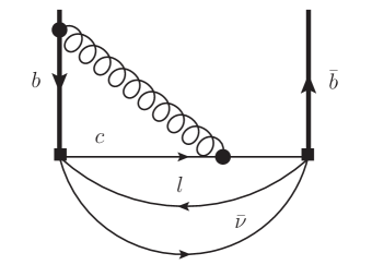
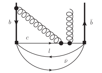
Figure 1: Diagrams for the contribution at NLO level, (left) - partonic type, right - power correction type with an insertion of an external gluon

The leading order result is given by two-loop Feynman integrals of a simple topology – the so called sunset-type diagrams [24, 25], while at the NLO level one has to evaluate three-loop integrals with massive lines due to the massive $c$- and $b$-quarks. In Fig. 1 we show a typical three-loop diagram for the power corrections in the heavy quark expansion.

We use dimensional regularization for both ultraviolet and infrared singularities. We used the systems of symbolic manipulations REDUCE [26] and Mathematica [27] with special codes written for the calculation. For reduction of integrals to master integrals the program LiteRed [28] was used. The master integrals have been then computed directly. Some of them have checked with the program HypExp [29].

For the Darwin term one takes an amplitude of quark to quark-gluon scattering and projects it to an HQET operator. We choose a momentum $k$ gluon and take the structure $(\epsilon v)k_{\perp}^{2}$. There are several operators in HQET that can have such a structure, for instance, ${\bar{h}}_{v}(\pi v)\pi_{\perp}^{2}h_{v}$. This operator is irrelevant because it is of higher power on shell. One disentangles the mixing of such operators with the Darwin term by using two quark momenta $k_{1}$ and $k_{2}$ and pick up the structure $(k_{1}k_{2})$ that emerges in the coefficient of the Darwin term. The other operators can have $k_{1}^{2}$ or $k_{2}^{2}$ structure. The coefficient $a_{D}$ is defined in front of the meson matrix element. After taking the matrix element one can use equation of motion of HQET to reduce the number of the operators in the basis. One more conventional step is to trade the leading order operator ${\bar{h}}_{v}h_{v}$ for the QCD operator ${\bar{b}}\not{v}b$ that provides correspondence to the parton model.

The final expression for the coefficient $a_{D}$ is then

$$a_{D} = 2(C_{D}+\frac{3}{4}(C_{v}C_{D}^{HQET}-C_{0}C_{D}^{bvb}))$$ (12)

where $C_{D}^{HQET}$ is the NLO coefficient of the operator $O_{D}$ in HQET Lagrangian, and $C_{D}^{bvb}$ is the NLO coefficient of the operator $O_{D}$ in the expansion of ${\bar{b}}\not{v}b$. At the LO we find

$$a_{D}^{LO}=-5r^{4}-8r^{3}+24r^{2}+36r^{2}\log(r)-88r+48\log(r)+77$$ (13)

where $r=m_{c}^{2}/m_{b}^{2}$ that agrees with [30]. The coefficient contains a logarithmic singularity $\log(r)$ at small $r$. This singularity reflects the mixing to hidden/intrinsic charm contribution [31]. At higher powers even more singular terms (like $1/r$) can appear [32]. The matching is performed by integrating out the charm quark simultaneously with the hard modes of the $b$-quark. This means that we treat $m_{c}^{2}/m_{b}^{2}$ as a number fixed in the limit $m_{b}\to\infty$, and therefore our results cannot be used to extrapolate to the limit $m_{c}\to 0$.

An important check of a loop computation consists in verifying the cancellation of poles after performing the appropriate renormalization of the physical quantity in question. Since in the case at hand this is quite delicate, we briefly discuss the renormalization of the $\rho_{D}$ coefficient at NLO within our computation.

We single out the pole contribution to the NLO coefficient in the form

$$C^{NLO}_{D}=\frac{\alpha_{s}(m_{b})}{4\pi}\left(\frac{1}{\epsilon}C^{NLO-pol}_{D}+C^{NLO-fin}_{D}\right)\,.$$ (14)

The contribution to the coefficient $C^{NLO-pol}_{D}$ from one-particle irreducible diagrams reads

$$C^{NLO-pol}_{D} = C_{A}\left(-\frac{17r^{4}}{3}+\frac{16r^{3}}{3}-28r^{2}+36r^{2}\log(r)+\frac{32r}{3}+16\log(r)+\frac{53}{3}\right)$$

$$+ C_{F}\left(-\frac{1181r^{4}}{8}+207r^{3}+87r^{2}+\frac{285}{2}r^{2}\log(r)-419r+72\log(r)+\frac{2181}{8}\right)\,.$$

The pole part of the coefficient $C^{NLO-pol}_{D}$ contains different functional dependencies on $r$, and it is instructive to see how the cancellation works in the present case.

The proper cancellation of these poles requires to consider the mixing between HQE operators of different dimensionality which is known to be possible in HQET [33, 34, 35, 36, 37, 38]. The anomalous dimensions of the operators are numbers independent of $r$ while the functions of $r$ appearing in $C_{D}$ should cancel in the renormalization of the coefficient. This is a rather strong restriction because only the coefficient functions of the lower power operators (which are basically $C_{0}(r)$ and $C_{v}(r)$) can be used for the pole cancellation in $C_{D}$. The leading order $C_{G}$ coefficient is proportional to $C_{0}^{LO}(r)$. Indeed, the explicit expression reads

$$C_{G}^{LO}=2-16r-24r^{2}\ln(r)+16r^{3}-2r^{4}=2C_{0}^{LO}\,.$$ (15)

These properties of HQE are important for the implementation of the renormalization procedure of the Darwin-term coefficient.

The operator ${\cal O}_{\pi}$ from HQE after the insertion of one more ${\cal O}_{\pi}$ from the Lagrangian can mix with ${\cal O}_{D}$ that produces the pole structure proportional to $C_{0}(r)$

$${\cal O}_{\pi}^{R}={\cal O}_{\pi}^{B}+\gamma_{\pi D}\frac{\alpha_{s}}{4\pi\epsilon}\frac{1}{m_{b}}{\cal O}_{D}\,.$$ (16)

The relation (16) means that the $ghh$ vertex computed in perturbation theory within HQET with one insertion of ${\cal O}_{\pi}$ gets a contribution from higher powers of the HQET Lagrangian (see, e.g. [33]). By the same token the operator ${\cal O}_{G}$ from HQE after the insertion of one more ${\cal O}_{G}$ from the Lagrangian can mix with ${\cal O}_{D}$

$${\cal O}_{G}^{R}={\cal O}_{G}^{B}+\gamma_{GD}\frac{\alpha_{s}}{4\pi\epsilon}\frac{1}{m_{b}}{\cal O}_{D}$$ (17)

that produces the pole structure proportional to $C_{0}(r)$ again because of eq. (15). The cross-insertions (${\cal O}_{G}$ from HQE to ${\cal O}_{\pi}$ from the Lagrangian and vice versa) renormalize the spin-orbit operator at the order $1/m_{b}^{2}$. This type of mixing is known for a long time from computation of $1/m_{b}^{2}$ running of coefficients of HQET Lagrangian.

In the literature the renormalization is considered often for the static heavy fields when the contributions of reiterated terms in the HQET Lagrangian are accounted for through the bi-local operators [36, 37]. We consider the standard approach and treat higher order terms as perturbations (see, [35, 39]). In our case the inclusion of these mixings does not suffice to cancel all the poles in $C_{D}$ as there are other structures than $C_{0}(r)$ necessary. The operator ${\cal O}_{v}$ can mix with double insertions of higher dimensional terms, i.e.

$${\cal O}_{v}^{R}={\cal O}_{v}^{B}+\gamma_{vD}\frac{\alpha_{s}}{4\pi\epsilon}\frac{1}{m_{b}^{2}}{\cal O}_{D}$$ (18)

and the counterterm proportional to ${\cal O}_{D}$ emerges from two insertions of the operators ${\cal O}_{\pi}$. The mixing matrix $\gamma_{vD}$ is unknown. But the effect of such a mixing leads to the appearance of the coefficient $C_{v}(r)$ in the expression for the poles. One can now fit the pole function with two entries $C_{0}(r)$ and $C_{v}(r)$.

Thus we infer the corresponding mixing anomalous dimensions and find that the combination

$$(-C_{A}+\frac{23}{8}C_{F})C_{v}(r)-(\frac{5}{4}C_{A}+\frac{31}{8}C_{F})C_{0}(r)$$ (19)

cancels the poles in both color structures $C_{F}$ and $C_{A}$ for the entire $m_{c}$ dependence. The solution in eq. (19) is unique. The presence of the coefficient $C_{v}$ means an admixture to the operator ${\cal O}_{v}$. At this level it is impossible to confirm the two mixings as the mixing matrices are still not uniquely given in the literature and $\gamma_{vD}$ is completely new. An independent computation of mixing matrices could be a useful check of our computation. Because the term $r^{2}$ is present only in the mixing with ${\cal O}_{v}$ one can extract $\gamma_{vD}$. But it is impossible to separate $\gamma_{mD}$ and $\gamma_{kD}$ as only their sum is extracted with our current method.

Thus we arrive at a finite coefficient for $\rho_{D}$, the analytical expression for NLO correction to $a_{D}$ is given in the Appendix. Here we discuss the numerical impact of our result. With $\alpha_{s}$ normalized at $m_{b}$ and for $r=m_{c}^{2}/m_{b}^{2}=0.07$ one finds

$$a_{D} = -57.159+\frac{\alpha_{s}(m_{b})}{4\pi}(-56.594C_{A}+408.746C_{F})$$ (20)

$$= -57.159+\frac{\alpha_{s}(m_{b})}{4\pi}(375.213)$$

$$= -57.159(1-\frac{\alpha_{s}}{4\pi}6.564\ldots)$$

For $\alpha_{s}(m_{b})=0.2$

$$a_{D} = -57.159(1-0.10)$$ (21)

the NLO contribution shifts the $\rho_{D}$ coefficient by 10%.

4 Discussion

The technical details of the calculation will be discussed in a more detailed paper, where we also plan to calculate moments of various distributions. However, the result presented here already have a few interesting consequences.

The first remark concerns the dependence on the mass of the charm quark which appears in the ratio $r=m_{c}^{2}/m_{b}^{2}$. This ratio is kept at a fixed value as $m_{b},m_{c}\to\infty$ and the behavior of the coefficients close to $r=0$ is given by

$$a_{D}^{LO} = -20(1-r)^{4}+\ldots$$ (22)

$$a_{D}^{NLO} = -C_{F}8(1-r)^{3}(29+312\ln(1-r))+\cdots$$ (23)

Note that the behaviour of the coefficient at the border of the available phase space depends on the definition of the $c$-quark mass. Here we use $\overline{\rm MS}$ mass. Ii Fig. 2 (left panel) we plot the dependence on $r$ in the full kinematically allowed region range $0\leq r\leq 1$. We show the ratio

$$\frac{a_{D}^{NLO}(1-r)}{a_{D}^{LO}}$$ (24)

while the right panel of Fig. 2 focuses on the physical region around $r=0.07$.

The plots show that the mass dependence in the physical region is weak, while it is sizable over the full range. As we discussed above, the massless limit cannot be taken, since in the case of a $b\to u$ transition additional operators have to be taken into account. Nevertheless at small $r$ the NLO corrections become even smaller and have a zero at $r\sim 0.005$. A similarly strong dependence has been observed also for the QCD corrections in the coefficient of $\mu_{G}^{2}$ [20].

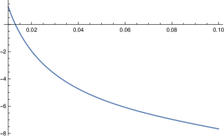
Figure 2: Mass dependence of the NLO Coefficient of $\rho_{D}$. Left panel: The ratio (24) over the full range of $r$, right panel: The ratio of the NLO coefficient to the LO one in the physically interesting region.

Although the corrections are not untypically large, they will have a visible impact on the determination of $V_{cb}$. This is mainly due to the fact that the coefficient in front of $\rho_{D}$ in the total rate is quite large, see (21). While a detailed analysis will require to repeat the combined fit as e.g. in [40] we may obtain a tendency from an approximate formula given in eq. (12) in this paper. According to (21) the NLO correction corresponds to a reduction of the contribution of $\rho_{D}$ by 10%, thus eq. (12) of [40] implies a shift in the central value of

$$\frac{\Delta V_{cb}}{V_{cb}}=-0.3\%\,,$$ (25)

which is about a third of the current theoretical uncertainty.

However, parametrically this correction is of the same size as the yet unknown corrections of order $\alpha_{s}^{2}\Lambda_{\rm QCD}^{2}/m_{b}^{2}$ and $\alpha_{s}^{3}$, which would need to be included in a full analysis up to order $\alpha_{s}\Lambda_{\rm QCD}^{3}/m_{b}^{3}$. We note in passing that the corrections $\alpha_{s}\rho_{LS}^{2}$ are not needed, since these are included in the known $\alpha_{s}\mu_{G}^{2}$ contributions [41]. Nevertheless, the contribution of $\rho_{D}$ is significant due to the large coefficient in front of $\rho_{D}$ and hence we expect that the impact of this correction is largest.

Acknowledgments
This research was supported by the Deutsche Forschungsgemeinschaft (DFG, German Research Foundation) under grant 396021762 - TRR 257 “Particle Physics Phenomenology after the Higgs Discovery”

5 Appendix

The matching coefficient of the “operator” $\rho_{D}$ in the HQET Lagrangian in NLO at $\mu=m_{b}$ gets a correction [12]

$$1+\frac{\alpha_{s}(m_{b})}{4\pi}2C_{A}\,.$$ (26)

After using equation of motions the final $\rho_{D}$-coefficient is expressed through the coefficient of the relevant operator in HQE (direct contribution) and the contributions due to HQET Lagrangian and the choice of the full QCD operator at the leading power through the relation

$$a_{D}=2\left\{C_{D}^{dir}+\frac{3}{4}C_{v}\left(1+\frac{\alpha_{s}}{4\pi}2C_{A}\right)-\frac{3}{4}C_{0}\right\}\,.$$ (27)

At LO one obtains

$$a_{D}^{LO}=-5r^{4}-8r^{3}+24r^{2}+36r^{2}\log(r)-88r+48\log(r)+77$$ (28)

that agrees with [30].

We write the coefficient of $\rho_{D}$ term after taking matrix elements as

$$a_{D}=a_{D}^{LO}+\frac{\alpha_{s}}{4\pi}a_{D}^{NLO}$$ (29)

and then

$$a_{D}^{NLO}=a_{D}^{NLO,cf}C_{F}+a_{D}^{NLO,ca}C_{A}\,.$$ (30)

The $C_{F}$ color part reads at NLO

$$a_{D}^{NLO,cf}=\left(-1776r^{5/2}-\frac{6464r^{3/2}}{3}-144r^{4}+120r^{2}-\frac{880\sqrt{r}}{3}\right)\text{Li}_{2}\left(-\sqrt{r}\right)+$$

$$\left(3408r^{5/2}+5312r^{3/2}-144r^{4}+120r^{2}+880\sqrt{r}\right)\text{Li}_{2}\left(\sqrt{r}\right)$$

$$+\left(168r^{4}+256r^{3}-1304r^{2}+928r+424\right)\text{Li}_{2}\left(\frac{r-1}{r}\right)$$

$$+\left(-408r^{5/2}-\frac{2368r^{3/2}}{3}-192r^{4}-32r^{3}+144r^{2}-\frac{440\sqrt{r}}{3}+80\right)\text{Li}_{2}(r)$$

$$-648\pi^{2}r^{5/2}-\frac{2800}{3}\pi^{2}r^{3/2}+44\pi^{2}r^{4}-\frac{1615r^{4}}{48}+\frac{16\pi^{2}r^{3}}{3}-\frac{123184r^{3}}{45}$$

$$-34\pi^{2}r^{2}-\frac{363827r^{2}}{180}$$

$$+\left(164r^{4}+\frac{880r^{3}}{3}-\frac{443r^{2}}{3}+584r+140\right)\log^{2}(r)$$

$$+\left(\frac{18677r^{4}}{15}-\frac{54296r^{3}}{45}+\frac{1648r^{2}}{9}+\frac{392}{15r^{2}}+\frac{6424r}{3}-\frac{4496}{45r}-\frac{20603}{9}\right)\log(1-r)$$

$$+\left(\left(1296r^{5/2}+\frac{5600r^{3/2}}{3}+\frac{880\sqrt{r}}{3}\right)\log\left(1-\sqrt{r}\right)\right.$$

$$+\left(-1296r^{5/2}-\frac{5600r^{3/2}}{3}-\frac{880\sqrt{r}}{3}\right)\log\left(\sqrt{r}+1\right)$$

$$-\frac{2093r^{4}}{60}+\frac{34466r^{3}}{45}+\frac{41815r^{2}}{18}$$

$$+\left(-296r^{4}-\frac{352r^{3}}{3}-\frac{6904r^{2}}{3}-576r-\frac{1912}{3}\right)\log(1-r)$$

$$\left.+\frac{3752r}{3}-\frac{2096}{3}\right)\log(r)+\frac{220204r}{45}-\frac{440\pi^{2}\sqrt{r}}{3}$$

$$+\frac{392}{15r}-\frac{40\pi^{2}}{3}-\frac{91603}{720}$$ (31)

Here $\text{Li}_{2}(z)$ is a dilogarithm.

The new master integral $N_{m}$ has appeared compared to our previous results. The relevant combination turns out to be $(N_{p}+N_{m})/2$, and both $N_{p}$ and $N_{m}$ should be evaluated at LO in $\epsilon$-expansion.

A similar expression for the $C_{A}$ color part of the NLO coefficient reads

$$a_{D}^{NLO,ca}=\left(-152r^{5/2}-\frac{400r^{3/2}}{3}-336r^{2}+\frac{280\sqrt{r}}{3}\right)\text{Li}_{2}\left(-\sqrt{r}\right)$$

$$+\left(456r^{5/2}+400r^{3/2}-336r^{2}-280\sqrt{r}\right)\text{Li}_{2}\left(\sqrt{r}\right)+$$

$$\left(-208r^{3}+\frac{712r^{2}}{3}-360r+216\right)\text{Li}_{2}\left(\frac{r-1}{r}\right)$$

$$+\left(-76r^{5/2}-\frac{200r^{3/2}}{3}-24r^{3}+72r^{2}-72r+\frac{140\sqrt{r}}{3}+24\right)\text{Li}_{2}(r)-$$

$$76\pi^{2}r^{5/2}-\frac{200}{3}\pi^{2}r^{3/2}+\frac{329r^{4}}{36}+4\pi^{2}r^{3}+\frac{749r^{3}}{9}+16\pi^{2}r^{2}+\frac{12941r^{2}}{45}+$$

$$\left(-\frac{172r^{3}}{3}+\frac{268r^{2}}{3}-216r+40\right)\log^{2}(r)+$$

$$\left(48r^{4}-\frac{10114r^{3}}{45}+134r^{2}+\frac{238}{15r^{2}}+\frac{280r}{3}-\frac{62}{r}-\frac{40}{9}\right)\log(1-r)+$$

$$\left(\left(152r^{5/2}+\frac{400r^{3/2}}{3}-\frac{280\sqrt{r}}{3}\right)\log\left(1-\sqrt{r}\right)+\left(-152r^{5/2}-\frac{400r^{3/2}}{3}+\frac{280\sqrt{r}}{3}\right)\log\left(\sqrt{r}+1\right)\right.$$

$$\left.-26r^{4}+\frac{11794r^{3}}{45}-673r^{2}+\left(\frac{136r^{3}}{3}-144r^{2}+128r-\frac{320}{3}\right)\log(1-r)+\frac{508r}{3}-\frac{1060}{3}\right)\log(r)+$$

$$12\pi^{2}r-\frac{2009r}{15}+\frac{140\pi^{2}\sqrt{r}}{3}+\frac{238}{15r}-4\pi^{2}-\frac{47137}{180}$$ (32)

Note that there is no $1/r$ singularity at small $r$. The small $r$ expansion for the $C_{F}$ structure is

$$a_{D}^{NLO,cf}=\left(-72\log^{2}(r)-\frac{2096\log(r)}{3}-84\pi^{2}-\frac{5815}{144}\right)-\frac{440\pi^{2}\sqrt{r}}{3}$$

$$+\frac{1}{9}r\left(1080\log^{2}(r)+7896\log(r)-1392\pi^{2}+80111\right)+O\left(r^{3/2}\right)$$ (33)

and for the $C_{A}$ part is

$$a_{D}^{NLO,ca}=\left(-68\log^{2}(r)-\frac{1060\log(r)}{3}-40\pi^{2}-\frac{7481}{36}\right)+\frac{140\pi^{2}\sqrt{r}}{3}$$

$$+r\left(-36\log^{2}(r)+\frac{740\log(r)}{3}+72\pi^{2}-\frac{2134}{9}\right)+O\left(r^{3/2}\right)$$ (34)

References

- [1] J. Charles, O. Deschamps, S. Descotes-Genon, H. Lacker, A. Menzel, S. Monteil, V. Niess and J. Ocariz et al., Phys. Rev. D 91, no. 7, 073007 (2015)
- [2] J. N. Butler et al. [Quark Flavor Physics Working Group Collaboration], arXiv:1311.1076 [hep-ex].
- [3] A. J. Bevan et al. [BaBar and Belle Collaborations], Eur. Phys. J. C 74, no. 11, 3026 (2014) [arXiv:1406.6311 [hep-ex]].
- [4] S. Forte, A. Nisati, G. Passarino, R. Tenchini, C. M. C. Calame, M. Chiesa, M. Cobal and G. Corcella et al., arXiv:1505.01279 [hep-ph].
- [5] M. A. Shifman and M. B. Voloshin, Sov. J. Nucl. Phys. 41, 120 (1985);
- [6] H. Georgi, Phys. Lett. B 240, 447 (1990);
- [7] M. Neubert, Phys. Rept. 245, 259 (1994);
- [8] A. V. Manohar and M. B. Wise, Camb. Monogr. Part. Phys. Nucl. Phys. Cosmol. 10, 1 (2000).
- [9] I. I. Y. Bigi, M. A. Shifman, N. G. Uraltsev and A. I. Vainshtein, Phys. Rev. Lett. 71, 496 (1993).
- [10] A. A. Penin and A. A. Pivovarov, Phys. Lett. B 443, 264 (1998) doi:10.1016/S0370-2693(98)01323-9 [hep-ph/9805344].
- [11] T. Mannel, W. Roberts and Z. Ryzak, Nucl. Phys. B 368, 204 (1992).
- [12] A. V. Manohar, Phys. Rev. D 56, 230 (1997)
- [13] D. Benson, I. I. Bigi, T. Mannel and N. Uraltsev, Nucl. Phys. B 665, 367 (2003).
- [14] T. van Ritbergen, Phys. Lett. B 454, 353 (1999) .
- [15] A. Pak and A. Czarnecki, Phys. Rev. Lett. 100, 241807 (2008).
- [16] K. Melnikov, Phys. Lett. B 666, 336 (2008).
- [17] T. Becher, H. Boos and E. Lunghi, JHEP 0712, 062 (2007) .
- [18] A. Alberti, P. Gambino and S. Nandi, JHEP, 1 (2014).
- [19] T. Mannel, A. A. Pivovarov and D. Rosenthal, Phys. Lett. B 741, 290 (2015) [arXiv:1405.5072 [hep-ph]].
- [20] T. Mannel, A. A. Pivovarov and D. Rosenthal, Phys. Rev. D 92, no. 5, 054025 (2015) doi:10.1103/PhysRevD.92.054025 [arXiv:1506.08167 [hep-ph]].
- [21] T. Mannel, A. A. Pivovarov and D. Rosenthal, Nucl. Part. Phys. Proc. 263-264, 44 (2015). doi:10.1016/j.nuclphysbps.2015.04.008
- [22] T. Mannel and K. K. Vos, JHEP 1806, 115 (2018) doi:10.1007/JHEP06(2018)115 [arXiv:1802.09409 [hep-ph]].
- [23] A. V. Manohar and M. B. Wise, Phys. Rev. D 49, 1310 (1994)
- [24] S. Groote, J. G. Korner and A. A. Pivovarov, Nucl. Phys. B 542, 515 (1999) doi:10.1016/S0550-3213(98)00812-8 [hep-ph/9806402].
- [25] S. Groote, J. G. Korner and A. A. Pivovarov, Annals Phys. 322, 2374 (2007); Phys. Lett. B 443, 269 (1998).
-
[26]
A. C. Hearn, REDUCE, User’s manual. Version 3.8.
Santa Monica, CA, USA. February 2004 - [27] Wolfram Research, Inc., Mathematica, Version 9.0, Champaign, IL (2012).
- [28] R. N. Lee, arXiv:1310.1145 [hep-ph].
- [29] T. Huber and D. Maitre, Comput. Phys. Commun. 178, 755 (2008).
- [30] M. Gremm and A. Kapustin, Phys. Rev. D 55, 6924 (1997) doi:10.1103/PhysRevD.55.6924 [hep-ph/9603448].
- [31] I. Bigi, T. Mannel, S. Turczyk and N. Uraltsev, JHEP 1004, 073 (2010) doi:10.1007/JHEP04(2010)073 [arXiv:0911.3322 [hep-ph]].
- [32] T. Mannel, S. Turczyk and N. Uraltsev, JHEP 1011, 109 (2010) doi:10.1007/JHEP11(2010)109 [arXiv:1009.4622 [hep-ph]].
- [33] A. F. Falk, B. Grinstein and M. E. Luke, Nucl. Phys. B 357, 185 (1991). doi:10.1016/0550-3213(91)90464-9
- [34] C. W. Bauer and A. V. Manohar, Phys. Rev. D 57, 337 (1998) doi:10.1103/PhysRevD.57.337 [hep-ph/9708306].
- [35] M. Finkemeier and M. McIrvin, Phys. Rev. D 55, 377 (1997) doi:10.1103/PhysRevD.55.377 [hep-ph/9607272].
- [36] C. Balzereit and T. Ohl, Phys. Lett. B 386, 335 (1996) doi:10.1016/0370-2693(96)00947-1 [hep-ph/9604352].
- [37] B. Blok, J. G. Korner, D. Pirjol and J. C. Rojas, Nucl. Phys. B 496, 358 (1997) doi:10.1016/S0550-3213(97)00202-2 [hep-ph/9607233].
- [38] C. L. Y. Lee, CALT-68-1663.
- [39] C. W. Bauer, A. F. Falk and M. E. Luke, Phys. Rev. D 54, 2097 (1996) doi:10.1103/PhysRevD.54.2097 [hep-ph/9604290].
- [40] P. Gambino and C. Schwanda, Phys. Rev. D 89, no. 1, 014022 (2014) doi:10.1103/PhysRevD.89.014022 [arXiv:1307.4551 [hep-ph]].
- [41] M. Fael, T. Mannel and K. Keri Vos, JHEP 1902, 177 (2019) doi:10.1007/JHEP02(2019)177 [arXiv:1812.07472 [hep-ph]].
- [42] J. G. Korner, F. Krajewski and A. A. Pivovarov, Phys. Rev. D 63, 036001 (2001) [hep-ph/0002166].
- [43] A. A. Penin and A. A. Pivovarov, Phys. Lett. B 435, 413 (1998) [hep-ph/9803363].