Elliptic special Weingarten surfaces of minimal type in $\mathbb{R}^{3}$ of finite total curvature

Abstract

We extend the theory of complete minimal surfaces in $\mathbb{R}^{3}$ of finite total curvature to the wider class of elliptic special Weingarten surfaces of finite total curvature; in particular, we extend the seminal works of L. Jorge and W. Meeks and R. Schoen.

Specifically, we extend the Jorge-Meeks formula relating the total curvature and the topology of the surface and we use it to classify planes as the only elliptic special Weingarten surfaces whose total curvature is less than $4\pi$. Moreover, we show that a complete (connected), embedded outside a compact set, elliptic special Weingarten surface of minimal type in $\mathbb{R}^{3}$ of finite total curvature and two ends is rotationally symmetric; in particular, it must be one of the rotational special catenoids described by R. Sa Earp and E. Toubiana. This answers in the positive a question posed in 1993 by R. Sa Earp. We also prove that the special catenoids are the only connected non-flat special Weingarten surfaces whose total curvature is less than $8\pi$.

^†Departamento de Matemática, Facultad de Ciencias, Universidad de Cádiz,
Puerto Real 11510, Spain
Email:josemaria.espinar@uca.es
^∗Instituto Nacional de Matemática Pura e Aplicada, 110 Estrada Dona Castorina,
Rio de Janeiro 22460-320, Brazil
Email: jespinar@impa.br
Email: hebermes@impa.br
^‡Departamento de Matemáticas, Universidad del Valle,
Santiago de Cali, Colombia
Email: heber.mesa@correounivalle.edu.co

Introduction

The study of minimal surfaces goes back to Lagrange and Euler in the XIX century and, today, is still one of the most fruitful fields in Geometric Analysis. Among minimal surfaces in the Euclidean space $\mathbb{R}^{3}$, those of finite total curvature, i.e., the Gaussian curvature is integrable, attracted considerable attention in the 80’s by authors as Osserman, Chern, Costa, Jorge, Meeks or Schoen (see [40] and references therein for a survey).

The Chern-Osserman theorem [13] asserts that such surfaces are conformally equivalent to a closed Riemann surface of finite genus with finitely punctures which correspond to the ends. In the seminal work of L. Jorge and W. Meeks [30], the authors established their famous formula that relates the total curvature with the topology of a minimal surface in $\mathbb{R}^{3}$ of finite total curvature as well as they studied the behavior of the ends of those surfaces; in particular, they proved that the only complete minimal surface of finite total curvature and one embedded end is the plane. These techniques were also used by R. Schoen [47] to prove one of the most remarkable theorems on the classification of minimal surfaces with finite total curvature in $\mathbb{R}^{3}$; the only complete (connected) minimal surface in $\mathbb{R}^{3}$ of finite total curvature and two embedded ends is the catenoid. Moreover, the Jorge-Meeks formula and the above results also classified the plane and the catenoid as the only complete minimal surfaces of finite total curvature, embedded ends and total curvature less than $8\pi$.

We focus in this paper on a wider class of surfaces in $\mathbb{R}^{3}$ that contains the family of minimal surfaces, elliptic special Weingarten surfaces, those that verify $H=f(H^{2}-K)$ for a certain function $f\in C^{0}([0,+\infty))\cap C^{1}((0,+\infty))$, here $H$ and $K$ are the mean and Gaussian curvatures, satisfying the elliptic condition

$$4tf^{\prime}(t)^{2}<1\text{ for all }t\in(0,+\infty).$$

Closed Weingarten surfaces in $\mathbb{R}^{3}$ were widely studied by P. Hartman and A. Wintner [22], S. Chern [11, 12], H. Hopf [28] and R. Bryant [8] obtaining, among others, a generalization of Hopf’s theorem and Liebmann’s theorem. In the case of non-compact special Weingarten surfaces, some condition on the function $f$ at $0$ and/or infinity are required in order to avoid pathological behaviors; in this paper we will impose the natural conditions in order that rotational examples behaving as catenoids, the special catenoids constructed by R. Sa Earp and E. Toubiana [43, 44], do exist.

Elliptic special Weingarten surfaces lived its golden age in the 90’s thanks to the seminal work of H. Rosenberg and R. Sa Earp [42] where they proved that this family satisfies the maximum principle, interior and boundary, and they can be divided into two types: constant mean curvature type if $f(0)\neq 0$; and minimal type if $f(0)=0$. We will focus in elliptic special Weingarten surfaces of minimal type, in short, ESWMT-surfaces.

Sa Earp and Toubiana in a serie of papers [43, 44] constructed rotationally symmetric examples; in particular what they called special catenoids; that behave as minimal catenoids in $\mathbb{R}^{3}$. These examples allowed them to extend the famous half-space theorem of Hoffman-Meeks [23] to the class of elliptic special Weingarten surfaces of minimal type. The authors also proved that the Gaussian curvature is non-positive, and its zeroes are isolated, and the convex hull property, all of them properties shared with minimal surfaces.

In [42], H. Rosenberg and R. Sa Earp focused on elliptic special Weingarten surfaces of constant mean curvature type, $f(0)\neq 0$, which means that the sphere of radius $1/|f(0)|$ belongs to this family. They were able to extend the Korevaar-Kusner-Meeks-Solomon theory [33, 35] for properly embedded constant mean curvature surfaces in $\mathbb{R}^{3}$ to this class of surfaces under additional conditions on $f$. When the mean curvature $H$ and the Gaussian curvature $K$ satisfy a linear relation, that is, when we are considering a Weingarten relation of the form $aH+bK=c$, where $a$, $b$ and $c$ are real constants, these surfaces are called linear Weingarten surfaces, abbreviated as LW-surfaces. Rosenberg and Sa Earp in [42] showed that if $b=1$ and $a,c>0$, the annular ends of a properly embedded LW-surface converge to Delaunay ends. Others results about elliptic special Weingarten surfaces can be consulted in [7, 20, 45, 46].

There was a gap of almost twenty years until J.A. Aledo, J.M. Espinar and J.A. Gálvez, [3] extended the Korevaar-Kusner-Meeks-Solomon theory without any additional hypothesis on $f$. The authors also classified elliptic special Weingarten surfaces, ESW-surfaces or $f$-surfaces in short, for which the Gaussian curvature $K$ does not change sign; results analogous to those due to T. Klotz and R. Osserman [32] for minimal surfaces. Specifically, they obtained that, if an ESW-surface is complete with $K\geq 0$ then it must be either a totally umbilical sphere, a plane or a right circular cylinder, and, if an ESW-surface is properly embedded with $K\leq 0$, then it is a right circular cylinder or $f(0)=0$, that is, it is of minimal type. In [21], Gálvez, Martínez and Teruel improved the above result in the case $K\leq 0$ replacing the properly embedded hypothesis by just completeness.

There is a lack of examples in the literature of ESW-surfaces in $\mathbb{R}^{3}$, most of them when the relation is linear [20, 42], for example D. Yoon and J. Lee, [53] construct helicoidal surfaces satisfying a linear Weingarten equation; however in the general case we only know the rotational examples constructed by R. Sa Earp and E. Toubiana mentioned above. We hope this work will be the starting point for fulfilling this gap in the near future.

Organization of the paper and main results

In this paper we study complete elliptic special Weingarten surfaces of minimal type in $\mathbb{R}^{3}$ of finite total curvature.

We begin Section 1 by establishing the preliminaries results we will use all along this paper; in particular the exact definition of elliptic especial Weingarten surface of minimal type we will consider. We will recall the results of Sa Earp and Toubiana in [44] that characterize the rotational examples of ESWMT-surfaces. Also, here we present the Weierstrass-Enneper representation for minimal surfaces and summarize Kenmotsu’s work [31] on the Gauss map of immersed surfaces in $\mathbb{R}^{3}$. We prove that an ESWMT-surface of finite total curvature must have finite total second fundamental form. We finish this section by defining an adapted Codazzi pair on an ESWMT-surface, which is based on the Weingarten relation, and pointing out that this pair satisfies a Simons type formula.

Section 2 is devoted to study the growth of the ends of an ESWMT-surface of finite total curvature. We prove that if the Gauss map at infinity is vertical and the end is the graph of a function defined outside some compact set in a horizontal plane then, after a vertical translation of the end if necessary, this function (the height function) is either positive or negative. As a consequence of this result we obtain that there are no non-planar one ended ESWMT-surfaces of finite total curvature in $\mathbb{R}^{3}$. Using the Kenmotsu representation we show that the height function is of logarithmic order, obtaining the regularity at infinity for ends of ESWMT-surfaces of finite total curvature.

In Section 3, we present a (new?) proof of the well known Jorge-Meeks formula for complete minimal surfaces of finite total curvature using the Simons formula. This approach and the adapted Codazzi pair defined in Section 1 allow us to extend this result to the family of complete ESWMT-surfaces of finite total curvature.

In Section 4, we extend the Alexandrov reflection method to unbounded domains of catenoidal type. We use it to show that a complete ESWMT-surface of finite total curvature with two ends and embedded outside a compact set must be rotational. This fact joined with the results of Sa Earp and Toubiana give us a Schoen type theorem for ESWMT-surfaces.

Finally, in Section 5, we use the Jorge-Meeks type formula to prove that planes and special catenoids are the only connected ESWMT-surfaces embedded outside a compact set whose total curvature is less than $8\pi$.

1 Preliminaries

We begin this section by recovering the basic facts on ESWMT-surfaces in $\mathbb{R}^{3}$ as well as the rotational examples given by R. Sa Earp and E. Toubiana [44]. Then, we shall recall the Kenmotsu representation [31] necessary for the description of the ends later on. Next, we justify the notion of finite total curvature and we will overview the previous results on this matter we will use. Finally, we remind the adapted Codazzi pair supported on a ESWMT-surface given in [3].

First, we will establish the notation we will use along this work. $\Sigma$ will denote a connected immersed oriented surface in $\mathbb{R}^{3}$, possibly with boundary, whose unit normal is denoted by $N$. Also, $I$, $II$, $H$, $K$, $q$, $k_{1}$ and $k_{2}$ denote the first fundamental form, second fundamental form, mean curvature, Gaussian curvature, skew curvature and principal curvatures respectively. Recall that the mean, Gaussian and skew curvatures are defined in terms of the principal curvatures as

$$2H=k_{1}+k_{2},\,\,K=k_{1}k_{2}\text{ and }q=H^{2}-K.$$

1.1 Elliptic special Weingarten surfaces of minimal type

We say that an oriented immersed (connected) surface $\Sigma$ is an ESWMT-surface in $\mathbb{R}^{3}$ if the mean curvature $H$ and Gaussian curvature $K$ satisfy a Weingarten relation of the form $H=f(H^{2}-K)$, where $f\in C^{0}([0,+\infty))\cap C^{1}((0,+\infty))$ verifying:

$$\left\{\begin{array}[]{l}f(0)=0\mbox{ and }4tf^{\prime}(t)^{2}<1\mbox{ for all }t\in(0,+\infty),\\[5.69054pt] f\text{ is non-negative},\\[5.69054pt] f\text{ is Lipschitz at }t=0,\\[5.69054pt] \displaystyle\liminf_{t\to 0^{+}}\,4tf^{\prime}(t)^{2}<1,\\[8.53581pt] \displaystyle\limsup_{t\to+\infty}\,4tf^{\prime}(t)^{2}<1.\end{array}\right.$$ (1)

Remark 1.

The conditions given in (1) are the natural ones, as we will see next, for the existence of a one parameter family of rotationally symmetric examples behaving as the family of minimal catenoids.

We will refer to the conditions in (1) as the elliptic conditions for the function $f$, and in the case that $f$ satisfies them we will say that $f$ is an elliptic function of minimal type. Elliptic means that the family of $f$-surfaces satisfies the maximum principle (interior and boundary) [7, 42]; hence, for ESW-surfaces we are able to apply the geometric comparison principle and the Alexandrov reflection method.

Note that trivially planes are ESWMT-surfaces for any $f$. Another observation to be made is that there is no closed ESWMT-surfaces in $\mathbb{R}^{3}$ by the maximum principle; in fact, ESWMT-surfaces and minimal surfaces share other properties (see [3, 43, 44]):

• the Gaussian curvature is non positive;

• the zeros of the Gaussian curvature of a non-flat ESWMT-surface are isolated;

• a point is umbilic if, and only if, the Gaussian curvature vanishes at this point;

• a compact ESWMT-surface is contained inside the convex hull of its boundary;

• planes are the only ESWMT-surfaces whose Gaussian curvature vanishes identically.

1.1.1 Rotationally symmetric examples

As examples of ESWMT-surfaces we have all minimal surfaces, this is for the specific case when $f\equiv 0$. In general, Sa Earp and Toubiana proved in [44] the existence and uniqueness of rotational ESWMT-surfaces assuming that the function $f$ satisfies

$$\liminf_{t\to 0^{+}}\,4tf^{\prime}(t)^{2}<1.$$ (2)

Remark 2.

Just in this subsection, $f$ elliptic means that $4tf^{\prime}(t)^{2}<1$ for all $t>0$. At each result, we will mention the extra hypothesis that $f$ must satisfy. We will do this since, at the end of this subsection, we will see how our definition adapts to the existence of special catenoids.

The first theorem about the existence of rotationally symmetric examples says:

Theorem 1 (Existence of rotational ESWMT-surfaces, [44]).

Let $f$ be an elliptic function satisfying $f(0)=0$ and (2), and let $\tau>0$ be a real number satisfying

$$\frac{1}{\tau}<\lim_{t\to\infty}\big{(}\sqrt{t}-f(t)\big{)}.$$ (3)

Then there exists a unique complete ESWMT-surface, $M_{\tau}$, satisfying $H=f(q)$ such that $M_{\tau}$ is of revolution. Moreover, the generatrix curve is the graph of a convex function of class $C^{3}$, strictly positive, with $\tau$ as a global minimum, and symmetric.

Theorem 1 determines pretty well the geometry of rotational examples of ESWMT-surfaces. We have two cases, if the generatrix lies or not in a strip orthogonal to the axis of revolution. In the first case, the ESWMT-surface $M_{\tau}$ lies between two parallel planes and, in the second case, all coordinates functions of $M_{\tau}$ are proper functions. See Figure 1.

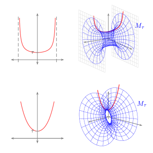
Figure 1: Generatrix (left) and complete ESWMT-surface $M_{\tau}$ (right).

Theorem 2 (Sa Earp-Toubiana, [44]).

Let $f$ be an elliptic function satisfying $f(0)=0$ and (2), and let $\tau>0$ be a real number satisfying (3). If $f$ is Lipschitz at $0$, then the ESWMT-surface $M_{\tau}$, obtained by Theorem 1, is not asymptotic to any plane in $\mathbb{R}^{3}$. Moreover, there exists a catenoid $C$ such that outside of a compact set, $M_{\tau}$ lies in the component of $\mathbb{R}^{3}\setminus C$ containing the revolution axis of $C$.

Theorem 3 (Sa Earp-Toubiana, [44]).

Let $f$ be a non-negative elliptic function satisfying $f(0)=0$ and (2). If $f$ is Lipschitz at $0$ and satisfies

$$\lim_{t\to\infty}\big{(}\sqrt{t}-f(t)\big{)}=+\infty,$$ (4)

then, as $\tau$ tends to $0$, the generatrix of $M_{\tau}$ tends to a ray orthogonal to the rotation axis.

Remark 3.

Our condition $\displaystyle\limsup_{t\to+\infty}\,4tf^{\prime}(t)^{2}<1$ in (1) implies (4).

The main consequence of the last theorem is that the family of ESWMT-surfaces $\left\{M_{\tau}:\tau>0\right\}$ behaves quite similar to the family of minimal catenoids. This means, in addition with the geometric comparison principle, that we have a half-space theorem for ESWMT-surfaces (with the appropriate requirements for $f$). The proof of this is the same as for minimal surfaces, see [23].

Corollary 1 (Half-space theorem for ESWMT-surfaces, [44]).

Let $f$ be a non-negative elliptic function Lipschitz at $0$ satisfying $f(0)=0$, (2) and (4). Let $\Sigma$ be a complete connected properly immersed ESWMT-surface verifying $H=f(q)$. If $\Sigma$ is contained in a half space of $\mathbb{R}^{3}$, then $\Sigma$ is flat.

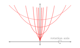
Figure 2: Generatrixes of rotational ESWMT-surfaces.

The uniqueness of these examples is obtained in the next theorem.

Theorem 4 (Sa Earp and Toubiana, [44]).

Let $f$ be an elliptic function satisfying $f(0)=0$ and (2). If $\Sigma$ is a complete ESWMT-surface satisfying $H=f(q)$ and rotationally symmetric, then there exists $\tau>0$ such that $\Sigma$ is the surface of revolution $M_{\tau}$ determined in Theorem 1.

1.2 Representation of surfaces in the Euclidean space

1.2.1 Weierstrass-Enneper representation

Let $(U,\mathbf{x}=(x,y))$ be a local chart of $\Sigma$, where $(x,y)$ are isothermal parameters for the first fundamental form, and consider the complex parameter $z=x+iy$, which is conformal, this is $I=2\lambda|dz|^{2}$. It is well known that $\Delta\mathbf{x}=2HN$, where $\Delta$ is the Laplace-Beltrami operator (see [15]). This allows us to conclude that $\Sigma$ is minimal in $\mathbb{R}^{3}$ if, and only if, the coordinate functions are harmonic.

We define

$$(\phi_{1},\phi_{2},\phi_{3})=\Phi=\partial_{z}\mathbf{x}\quad\mbox{and}\quad((\Phi,\Phi))=\phi_{1}^{2}+\phi_{2}^{2}+\phi_{3}^{2}.$$

A straightforward computation shows that $z$ is a conformal parameter if, and only if, $((\Phi,\Phi))=0$, and $\Delta\mathbf{x}=0$ if, and only if, $\partial_{\bar{z}}\Phi=0$, see [39]. Note that the condition $\partial_{\bar{z}}\Phi=0$ says that all the components of $\Phi$ are holomorphic, and in this case we will say that $\Phi$ is holomorphic.

We can recover the immersion $\mathbf{x}$, on simply connected domains, from $\Phi$ by Cauchy’s theorem as

$$\mathbf{x}(z)=\Re\left\{\int_{z_{0}}^{z}\Phi(w)\,dw\right\},$$

then, in order to get locally minimal surfaces, we focus on holomorphic solutions of the equation $((\Phi,\Phi))=0$. The next lemma characterizes those solutions.

Lemma 1 (Osserman, [39]).

Let $U\subset\mathbb{C}$ be a domain and $g:U\rightarrow\mathbb{C}$ a meromorphic function. Let $f:U\rightarrow\mathbb{C}$ be a holomorphic function having the property that each pole of $g$ of order $m$ is a zero of order at least $2m$. Then,

$$\Phi=\left(\frac{1}{2}f(1-g^{2}),\frac{i}{2}f(1+g^{2}),fg\right)$$ (5)

is holomorphic and satisfies $((\Phi,\Phi))=0$. Conversely, every holomorphic $\Phi$ satisfying $((\Phi,\Phi))=0$ may be represented in the form (5), except for $\Phi=(\phi,-i\phi,0)$.

The lemma above implies the next theorem which gives us a local representation of minimal surfaces in $\mathbb{R}^{3}$.

Theorem 5 (Weierstrass-Enneper representation).

Every minimal surface immersed in $\mathbb{R}^{3}$ can be locally represented in the form

$$\mathbf{x}(z)=\Re\left\{\int_{0}^{z}\Phi(\omega)\,d\omega\right\}+c$$ (6)

where $c$ is a constant in $\mathbb{R}^{3}$, $\Phi$ is defined by (5), the functions $(f,g)$ having the properties stated in Lemma 1, the domain $U$ being the unit disk, and the integral being taken along an arbitrary path from the origin to the point $z$. The surface $\mathbf{x}(U)$ will be regular if, and only if, $f$ vanishes only at the poles of $g$, and the order of each zero is exactly twice the order of this point as pole of $g$.

Remark 4.

It is easy to check that if an immersed minimal surface is represented by (6), the Gauss map is exactly the meromorphic function $g$.

1.2.2 Kenmotsu representation

A natural question is: can we generalize the Weierstrass-Enneper representation for any other kind of surface? The answer is yes, we can have a representation quite similar to the Weierstrass-Enneper one for any immersed surface in $\mathbb{R}^{3}$, however, the complex functions involved in the representation may not be holomorphic. One of this kind of representations was presented by Kenmotsu in [31].

Let $\Sigma$ be an oriented surface immersed in $\mathbb{R}^{3}$ and $z=x+iy$ be a conformal parameter for the first fundamental form, $I$. We consider the smooth unit normal vector field $N$ defined by $N=\frac{1}{|\partial_{x}\wedge\partial_{y}|}\left(\partial_{x}\wedge\partial_{y}\right)$, where $\wedge$ is the exterior product in $\mathbb{R}^{3}$. Consider the stereographic projection of the unit normal $N=(N_{1},N_{2},N_{3})$ from the north pole, that is,

$$g(z)=\frac{N_{1}(z)}{1-N_{3}(z)}+i\frac{N_{2}(z)}{1-N_{3}(z)}.$$

We will call this function, again, the Gauss map of the surface $\Sigma$. Hence,

$$N=\frac{1}{1+g\bar{g}}\left(g+\bar{g},-i\left(g-\bar{g}\right),-1+g\bar{g}\right),$$

and $N_{z}=g_{z}\bar{\xi}+\bar{g}_{z}\xi$, where $\xi$ is the vector field defined as

$$\xi=\frac{1}{(1+g\bar{g})^{2}}\big{(}1-g^{2},i(1+g^{2}),2g\big{)}.$$

The tangent vector field $\partial_{z}$ can be obtained from the Gauss map $g$ as

$$\partial_{z}=-\frac{1}{H}\bar{g}_{z}\xi,$$ (7)

and then, as in the minimal case, we can recover the immersion $\mathbf{x}$, on simply connected domains, by integration.

From (7) and the Codazzi equation we have that the Gauss map of the immersion is a solution of the next differential equations.

Theorem 6 (Kenmotsu, [31]).

The Gauss map $g$ of an immersed surface $\Sigma$ in $\mathbb{R}^{3}$ must satisfy

$$Hg_{z}=\frac{Q}{\lambda}g_{\bar{z}},$$ (8)

$$H\left(g_{z\bar{z}}-\frac{2\bar{g}}{1+g\bar{g}}g_{z}g_{\bar{z}}\right)=H_{z}g_{\bar{z}},$$ (9)

where $\lambda$ is the conformal factor, $Q$ is the $(2,0)-$part of the second fundamental form, $Q=II(\partial_{z},\partial_{z})$, and $H$ is the mean curvature of the immersion.

On the one hand, note that when the immersion is minimal, the Beltrami equation (8) implies that $g_{\bar{z}}=0$, which means that the Gauss map is a holomorphic function; this fact was pointed by Osserman in [39]. Hence, (8) can be seen as a generalization of the Cauchy-Riemann equations for $g$ in the minimal case. On the other hand, the second order differential equation (9) is a complete integrability condition for the equation (7).

We have now all the elements to recover the immersion from the Gauss map and the non-zero mean curvature. This means that we can have a representation formula for immersed surfaces prescribing the mean curvature and the Gauss map. Such representation, presented bellow, can be seen as a generalization of the Weierstrass-Enneper formula for minimal surfaces.

Theorem 7 (Kenmotsu representation, [31]).

Let $\Sigma$ be a simply connected $2$-dimensional smooth manifold and $H:\Sigma\rightarrow\mathbb{R}$ be a non-zero $C^{1}-$function. Let $g:\Sigma\rightarrow\mathbb{C}\cup\{\infty\}$ be a smooth map satisfying (9) for $H$. Then there exists a branched immersion $\mathbf{x}:\Sigma\rightarrow\mathbb{R}^{3}$ with Gauss map $g$ and mean curvature $H$. Moreover, the immersion is unique up to similarity transformations of $\mathbb{R}^{3}$ and it can be recovered using the equation

$$\mathbf{x}=\Re\left\{\int-\frac{1}{H}\bar{g}_{z}\xi\,dz\right\}+c,$$ (10)

where $c$ is a constant in $\mathbb{R}^{3}$ and the integrals are taken along a path from a fixed point to a variable point. Moreover, if $g_{\bar{z}}\neq 0$, then $\mathbf{x}(\Sigma)$ is a regular surface.

1.3 Finite total curvature

A complete immersed surface $\Sigma$ in $\mathbb{R}^{3}$ has finite total curvature if its Gaussian curvature is integrable, that is,

$$\left|\int_{\Sigma}K\,dA\right|<+\infty.$$

In [38], R. Osserman showed that for minimal surfaces in $\mathbb{R}^{3}$ the total curvature is related to the distribution of the normals, specifically he proved that if a complete minimal surface has finite total curvature, then the surface is conformally equivalent to a compact Riemann surface with a finite number of points removed, and the Gauss map extends to a meromorphic function in those points. It is possible to obtain a similar Osserman’s theorem avoiding the minimal hypothesis. The topological conclusion can be deduced without the minimal hypothesis, this was achieved by A. Huber in [29]; the second implication was obtained by B. White in [52] assuming finite total second fundamental form and Gaussian curvature non positive.

Theorem 8 (B. White, [52]).

If $\int_{\Sigma}|II|^{2}\,dA<+\infty$ then $\Sigma$ has finite total curvature, in particular $\Sigma$ is of finite conformal type, this is, $\Sigma$ is conformally diffeomorphic to $\overline{\Sigma}\setminus\{p_{1},\ldots,p_{k}\}$, where $\overline{\Sigma}$ is a compact Riemann surface. If in addition $K$ is non positive, then $\Sigma$ is properly immersed and the Gauss map extends continuously to all $\overline{\Sigma}$, and any end is a multigraph over some plane. Moreover, if an end is embedded, this end is a graph over some plane.

As mentioned above, finite total curvature does not ensure a good control on the ends; however the ellipticity conditions (1) and finite total curvature will imply finite total second fundamental form. Hence, by White’s theorem (Theorem 8), we will be able to control the conformal type and ensure that the ends are graphical.

Lemma 2.

Let $\Sigma\subset\mathbb{R}^{3}$ be a complete ESWMT-surface satisfying (1) of finite total curvature; then it has finite total second fundamental form. Moreover,

$$\lim_{\left|y_{i}\right|\to+\infty}\left|II\right|=0,$$

for any proper sequence $y_{i}\in\Sigma$.

Proof.

From (1), since $f$ is Lipschitz at $t=0$, there exists $\delta>0$ and $C>0$ so that $f(t)\leq Ct$ for all $t\in[0,\delta]$. Consider $\epsilon<{\rm min}\left\{\delta/2,C^{-2}/2\right\}$, then there exists $0<c(\epsilon)<1$ so that $f(t)\leq c_{1}\sqrt{t}$ for all $t\in[0,\epsilon]$; moreover $c(\epsilon)\to 0$ as $\epsilon\to 0$.

Since $4tf^{\prime}(t)^{2}<1$ for all $t\in\mathbb{R}^{+}$ and $\displaystyle\limsup_{t\to+\infty}\,4tf^{\prime}(t)^{2}<1$, there exists a constant $c(\bar{t})<1$ so that $f(t)\leq f(\epsilon)-c(\bar{t})\sqrt{\epsilon}+c(\bar{t})\sqrt{t}$ for all $t\in[\epsilon,+\infty]$. Finally, there exists ${\rm max}\left\{c(\epsilon),c(\bar{t})\right\}<\bar{c}<1$ so that $f(t)\leq\bar{c}\sqrt{t}$ for all $t\in\mathbb{R}^{+}_{0}$.

Let $E\subset\Sigma$ be an end, which is conformally equivalent to a punctured disk $\mathbb{D}^{*}:=\mathbb{D}\setminus\left\{0\right\}$ by Huber’s theorem [29]. Then,

$$\int_{\mathbb{D}^{*}}H^{2}\,dA=\int_{\mathbb{D}^{*}}f^{2}(H^{2}-K)\,dA\leq\bar{c}^{2}\int_{\mathbb{D}^{*}}\big{(}H^{2}-K\big{)}\,dA,$$

that is,

$$(1-\bar{c}^{2})\int_{\mathbb{D}^{*}}H^{2}\,dA\leq-\bar{c}^{2}\int_{\mathbb{D}^{*}}K\,dA<+\infty;$$

which implies that

$$\int_{\Sigma}|II|^{2}\,dA<+\infty,$$

as claimed.

Let us see now that the second fundamental form goes to zero at infinity. Let $E\subset\Sigma$ be such an end in the conditions above; by Theorem 8, up a rotation, $E$ is a multi-graph over the plane $P:=\left\{p\in\mathbb{R}^{3}\,:\,\,\langle p,e_{3}\rangle=0\right\}$, where $e_{3}=\displaystyle\lim_{i\to+\infty}N(y_{i})$ for any sequence $y_{i}\in E$ so that $\left|y_{i}\right|\to+\infty$; here $N$ is the normal of the surface.

Assume that there exists a sequence $y_{i}\in E$, $\left|y_{i}\right|\to+\infty$, so that $\left|II\right|\not\to 0$. Let $x_{i}\in P$ be the points $y_{i}$ projected onto $P$. Since $E$ is proper, up to a subsequence, we can find $\delta>0$ so that the disks $D_{i}:=D(x_{i},\delta)\subset P$ are pairwise disjoint; denote by $\mathcal{D}_{i}\subset\Sigma$ the graph that projects onto $D_{i}$. By abuse of notation, we still denote by $\mathcal{D}_{i}$ the translation that takes $y_{i}$ onto the origin. If the second fundamental form does not go zero along this sequence, we would be able to find a sequence $\tilde{y}_{i}\in\mathcal{D}_{i}$ so that $N(\tilde{y}_{i})\not\to e_{3}$; which contradicts that the Gauss map extends continuously. ∎

Remark 5.

In order to prove Lemma 2, we do not need to assume that $f$ is non-negative in (1).

Remark 6.

In [52], B. White proved that any complete surface immersed in $\mathbb{R}^{3}$ of finite total second fundamental form has finite total curvature. This result and Lemma 2 show that these conditions are equivalent for ESWMT-surfaces, in the same way that they are equivalent for minimal surfaces.

1.4 Adapted Codazzi pair

A Codazzi pair on a surface is, in a few words, a pair of symmetric bilinear forms $(A,B)$ satisfying a Codazzi type equation being $A$ positive definite. In the particular case of a immersed surface in $\mathbb{R}^{3}$, the pair $(I,II)$ given by the first and the second fundamental forms of the immersion is a Codazzi pair (see [3] and references therein).

Remark 7.

The results in this subsection are contained in [3] and, most of them, only use the Weingarten relation $H=f(H^{2}-K)$. However, we will state all the results for ESWMT-surfaces.

Consider a ESWMT-surface $\Sigma$ and the pair $(I,II)$ given by the fundamental forms of the immersion. Around any non umbilical point, or any interior umbilical point, there exist local parameters $(u,v)$, given by lines of curvature, such that we are able to write

$$\begin{array}[]{lll}I&=&Edu^{2}+Gdv^{2},\\[5.69054pt] II&=&k_{1}Edu^{2}+k_{2}Gdv^{2}.\end{array}$$

In these coordinates, the Codazzi equations satisfied by the fundamental pair are equivalent to the following equations:

$$(k_{1})_{v}E=-tE_{v}\text{ and }(k_{2})_{u}G=tG_{u},$$

where $t=\frac{1}{2}(k_{1}-k_{2})$. Note that $t^{2}=q=H^{2}-K$.

Now we will use the relation $H=f(H^{2}-K)$ in order to get a new Codazzi pair on the ESWMT-surface $\Sigma$. Set $\phi(r)=\int_{0}^{r}2f^{\prime}(s^{2})ds$ and define the following symmetric bilinear forms:

$$\begin{array}[]{lll}I_{f}&=&\left(\cosh\phi(\sqrt{q})-H\frac{\sinh\phi(\sqrt{q})}{\sqrt{q}}\right)I+\frac{\sinh\phi(\sqrt{q})}{\sqrt{q}}II,\\[5.69054pt] II_{f}&=&\left(-H\cosh\phi(\sqrt{q})+\sqrt{q}\sinh\phi(\sqrt{q})\right)I+\cosh\phi(\sqrt{q})II.\end{array}$$ (11)

A quick computation shows that the mean curvature, the extrinsic curvature, and the skew curvature of this pair are $H_{f}=0$, $\mathcal{K}_{f}=-t^{2}=-(H^{2}-K)=-q$ and $q_{f}=q$, respectively.

Lemma 3 (Aledo-Espinar-Gálvez, [3]).

If $\Sigma$ is a ESWMT-surface satisfying $H=f(H^{2}-K)$, then $(I_{f},II_{f})$ is a Codazzi pair on $\Sigma$. In particular, the $(2,0)-$part of $II_{f}$ is holomorphic with respect to the conformal structure given by $I_{f}$.

The pair $(I_{f},II_{f})$ can be defined globally on $\Sigma$; note that at an umbilic point $I_{f}=I$ and $II_{f}\equiv 0$ (see [3]). It is important to note that the umbilic points of $(I,II)$ coincide with the umbilic points of $(I_{f},II_{f})$ since $q=q_{f}$. Moreover, the Codazzi pair $(I_{f},II_{f})$ satisfies the Simons type formula (cf. [36]):

$$\Delta^{I_{f}}\ln|II_{f}|=2\mathcal{K}_{f}\text{ away from the umbilic points},$$ (12)

where $\Delta^{I_{f}}$ and $|II_{f}|$ are the laplacian w.r.t. the metric $I_{f}$ and the norm of $II_{f}$ respectively. Here, $\mathcal{K}_{f}$ is the Gaussian curvature of $I_{f}$.

2 Growth of an ESWMT-end of finite total curvature

By Theorem 8 and Lemma 2 we know that the embedded ends of an ESWMT-surface of finite total curvature are, outside of some compact set, graphs of functions defined over planes orthogonal to the Gauss map at infinity. We will prove that each of these functions cannot grow infinitely in opposite directions, this is, after a translation of the end we can consider each function either non-negative or non-positive. Using this fact we are able to use some results of S. Taliaferro about the growth of a positive superharmonic function near an isolated singularity, see [49, 50], for obtaining a Bôcher type theorem that gives us a full description of the height function defined on a conformal parameter. In order to describe the growth of the ends in cartesian coordinates we use the Kenmotsu representation obtaining a kind of regularity at infinity for the ends in the sense of Schoen [47].

2.1 The height function

Let $E\subset\Sigma$ be an embedded end and suppose that the Gauss map goes (at this end) to the unitary vector $\nu\in\mathbb{R}^{3}$ at infinity. We define the plane $\Pi_{\nu}=\{x\in\mathbb{R}^{3}:\langle x,\nu\rangle=0\}$. By Theorem 8 we can write $E=\{x+\phi(x)\nu:x\in\Pi_{\nu}\setminus B_{\Pi_{\nu}}(R)\}$ for some smooth function $\phi:\Pi_{\nu}\setminus B_{\Pi_{\nu}}(R)\rightarrow\mathbb{R}$, where $B_{\Pi_{\nu}}(R)=\{x\in\Pi_{\nu}:||x||\leq R\}$. We denote by $N:E\rightarrow\mathbb{S}^{2}$ the Gauss map and $\theta:E\rightarrow[-1,1]\subset\mathbb{R}$ the angle function defined by $\theta(x)=\langle N(x),\nu\rangle$ for each $x\in E$. By the continuity of the Gauss map at infinity there exists $0<\epsilon<1$ such that $1-\epsilon\leq\theta(x)\leq 1$ for all $x\in E$. Let $\iota:E\rightarrow\mathbb{R}^{3}$ be the inclusion map, then it is well known that $\Delta^{E}\iota=2\mathbf{H}$, where $\mathbf{H}$ is the mean curvature vector of $E$, that is, $\mathbf{H}=HN$, $H$ the mean curvature and $\Delta^{E}$ the Laplacian operator on $E$. Multiplying by $\nu$ this identity we get $\Delta^{E}\langle\iota,\nu\rangle=2H\theta$, and abusing notation we write $\langle\iota,\nu\rangle=\phi$ and $\Delta^{E}\phi=2H\theta$.

By Huber’s theorem [29] the end $E$ is conformally equivalent to the punctured disk $\mathbb{D}^{*}$, that is, there exists a diffeomorphism $\alpha:\mathbb{D}^{*}\rightarrow E$ such that the metrics $g_{0}$ and $g_{1}=\alpha^{*}g$ are pointwise conformal. Here we are denoting as $g_{0}$ and $g$, the flat metric in $\mathbb{D}^{*}$ and the Euclidean metric restricted to $E$, respectively. It follows that there exists a smooth positive function $\lambda:\mathbb{D}^{*}\rightarrow\mathbb{R}$ such that we can write $g_{1}=\lambda g_{0}$, and, after a straightforward computation, $\Delta^{g_{1}}=\lambda^{-1}\Delta^{g_{0}}$. Define the function $u:\mathbb{D}^{*}\rightarrow\mathbb{R}$ by $u(z)=\langle\alpha(z),\nu\rangle$, due to the fact that $\alpha$ is an isometry from $(\mathbb{D}^{*},g_{1})$ onto $(E,g)$ we have that $\Delta^{g_{1}}u=(\Delta^{E}\langle\iota,\nu\rangle)\circ\alpha$; joining this with the relation between the Laplacians and the expression obtained for $\Delta^{E}\phi$ we achieve

$$\Delta^{g_{0}}u=2\lambda H\theta.$$ (13)

We think on the function $u$ as the height of the end $E$, over the plane $\Pi_{\nu}$, given by the conformal immersion $\alpha:\mathbb{D}^{*}\rightarrow E$, see Figure 3.

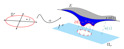
Figure 3: Parametrizing the end $E$ with a conformal parameter.

The first claim about the height function $u$ of an end $E$ is that, after a vertical translation of the end $E$, either $u\geq 0$ or $u\leq 0$. This means that the end $E$ cannot grow infinitely in both directions $\nu$ and $-\nu$ simultaneously. Specifically, we are going to prove the follow lemma.

Lemma 4 (Growth lemma).

Let $E$ be an embedded end of an immersed ESWMT-surface $\Sigma$. Suppose there exists $R>0$ such that $E$ is obtained as the graph of a $C^{2}$ class function $\phi$ defined in $\mathbb{R}^{2}\setminus B(R)$. Suppose also that $|\nabla\phi|\to 0$ as $r\to\infty$, where $r$ is the distance from an arbitrary point to the origin. Then at least one of the quantities $\displaystyle\inf_{|(x,y)|\geq R}\phi(x,y)$ or $\displaystyle\sup_{|(x,y)|\geq R}\phi(x,y)$ is finite.

Remark 8.

In order to prove Lemma 4, we only need to impose that the elliptic function $f$ satisfies $4tf^{\prime}(t)<1$ for all $t\in(0,+\infty)$ and $f(0)=0$; that is, we do not need to impose all the conditions on (1).

The proof presented here is based principally on the work of H. Chan [9, 10], S. Bernstein [6] and E. Hopf [25], and it is based in several lemmas that we are going to introduce.

Consider a circle $\gamma$ contained in the domain of $\phi$. Let $P_{\gamma}$ denote the linear function that best approximates the function $\phi$ on the circle $\gamma$ in the supremum norm. If we define

$$m(\gamma)=\inf_{a,b,c\in\mathbb{R}}\left\{\sup_{(x,y)\in\gamma}\left|\phi(x,y)-(ax+by+c)\right|\right\},$$ (14)

then $\displaystyle m(\gamma)=\sup_{(x,y)\in\gamma}\left|\phi(x,y)-P_{\gamma}(x,y)\right|$. Note that $m(\gamma)=0$ if, and only if, $\left\{\phi(x,y)\,:\,\,(x,y)\in\gamma\right\}$ is a planar curve.

The next lemma, under the hypothesis that $\phi$ is not linear, guaranties the existence of a circle such that its best approximating plane is not horizontal.

Lemma 5 (Chan-Treibergs, [10]).

If $\phi$ is not a linear function, there exists a circle $\gamma_{0}$ surrounding $\partial B(R)$ such that $m(\gamma_{0})\neq 0$ and $\nabla P_{\gamma_{0}}\neq 0$.

The Tchebychev equioscillation theorem, see [1, p. 57], says that if a polynomial of degree $n$ is the best approximation of a function defined on a compact interval, in the supremum norm, then there exist at least $n+2$ ordered points on the interval where this distance is attained and the polynomial oscillates around the function. There is a special version of the Tchebychev equioscillation theorem for periodic functions approximated by trigonometric functions, see [1, pp. 64–65]. This version immediately guaranties the following lemma.

Lemma 6.

For any circle $\gamma$ contained in the domain of $\phi$, there exist at least four points, ordered as, $\beta_{1}^{+}$, $\beta_{1}^{-}$, $\beta_{2}^{+}$, $\beta_{2}^{-}$ along $\gamma$, such that for $i=1,2$ we have $\phi(\beta_{i}^{+})=P_{\gamma}(\beta_{i}^{+})+m(\gamma)$ and $\phi(\beta_{i}^{-})=P_{\gamma}(\beta_{i}^{-})-m(\gamma)$.

This lemma means that on the circle $\gamma$ the function $\phi-P_{\gamma}$ alternates between $m(\gamma)$ and $-m(\gamma)$ at the points $\beta_{i}^{\pm}$, see Figure 4.

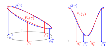
Figure 4: The Tchebychev theorem.

The next lemma is due to S. Bernstein and it was used by him to prove the famous Bernstein’s theorem about entire minimal graphs.

Lemma 7 (Bernstein, [6]).

Let $\phi$ be of class $C^{2}$ in a connected open set $\Omega$ and let $\phi_{xx}\phi_{yy}-\phi_{xy}^{2}\leq 0$ in $\Omega$. Assume $\phi>0$ in $\Omega$ and $\phi=0$ on $\partial\Omega$. Suppose that $\Omega$ can be placed in a sector of angle less than $\pi$. Let $M(r)$ be the maximum of $\phi$ on the part of the circle of radius $r$, centered at some fixed point, contained in $\overline{\Omega}$. Then there exist a positive constant $c$ such that $M(r)>cr$ for all $r$ sufficiently large.

The original proof of Bernstein of his theorem contained a gap. E. Hopf [26] proved a topological lemma, which is the key to fulfill the gap detected in Bernstein’s work. This lemma is also important in the proof of our result and it reads as follows.

Lemma 8 (Hopf, [26]).

If $\Omega\subset\mathbb{R}^{n}$ is a bounded open set and $\Omega^{\prime}\subset\Omega$ is a connected open subset whose boundary has at least one point in common with $\partial\Omega$, then the set $\partial\Sigma\cap\partial\Sigma^{\prime}$ of all of these common boundary points contains a set accessible from within $\Omega$. If $\partial\Sigma\cap\partial\Sigma^{\prime}$ is the union of two disjoint closed sets then each of these sets contains a set accessible from within $\Omega$.

Proof of the growth lemma.

The Gaussian curvature $K$ of $E$ is then given by

$$K=\frac{\phi_{xx}\phi_{yy}-\phi_{xy}^{2}}{(1+\phi_{x}^{2}+\phi_{y}^{2})^{2}},$$

therefore the function $\phi$ satisfies $\phi_{xx}\phi_{yy}-\phi_{xy}^{2}\leq 0$. If $K$ vanishes identically, then $E$ is contained in a plane and, hence, $\phi$ is linear. From the hypothesis on the gradient of $\phi$, we conclude that $\phi\equiv 0$, and the lemma is proven. Consequently we will consider that $K$ does not vanish identically.

Now, assume that

$$\inf_{|(x,y)|\geq R}\phi(x,y)=-\infty\mbox{ \ and \ }\displaystyle\sup_{|(x,y)|\geq R}\phi(x,y)=\infty,$$ (15)

with the purpose of obtaining a contradiction.

Claim A.

The function $\phi$ has sublinear growth.

Proof of Claim A.

For $r\geq R$, let $\gamma(r)$ be the circle centered at the origin and radius $r$, $m(r)$ and $M(r)$ be the minimum and the maximum value of $\phi$ on $\gamma(r)$ respectively. Taking $r$ large enough, (15) implies that

$$m(r)<\min\left\{0,m(R)\right\}\mbox{ \ and \ }M(r)>\max\left\{0,M(R)\right\}.$$

By Lemma 6, there exist ordered points $p_{1},q_{1},p_{2},q_{2}$ in $\gamma(r)$ such that $\phi(p_{1})=m(r)$, $\phi(p_{2})=M(r)$ and $\phi(q_{1})=\phi(q_{2})=0$. By the mean value theorem, there exist points $w_{1},w_{2}$ in $\gamma(r)$ such that

$$-m(r)=|\phi(p_{1})-\phi(q_{1})|\leq\pi r|\nabla\phi(w_{1})|,$$

$$M(r)=|\phi(p_{2})-\phi(q_{2})|\leq\pi r|\nabla\phi(w_{2})|.$$

Thus, for any $p$ in $\gamma(r)$, we have

$$-r\epsilon(r)\leq-\pi r|\nabla\phi(w_{1})|\leq m(r)\leq\phi(p)\leq M(r)\leq\pi r|\nabla\phi(w_{2})|\leq r\epsilon(r),$$

where $\displaystyle\epsilon(r)=\frac{1}{\pi}\max_{\gamma(r)}|\nabla\phi|$.

To obtain a non-increasing function $\epsilon(r)$ and the strict inequality it is sufficient to change $\epsilon(r)$ by $\sup\{\epsilon(\bar{r}):\bar{r}\geq r\}+\frac{1}{r^{2}}$; this proves Claim A. ∎

From now on, we redefine $R$, if necessary, in order to argue that the function $\phi$ has sublinear growth in $\mathbb{R}^{2}\setminus B(R)$.

According to Lemma 5, there exists a circle $\gamma_{0}$ of radius $r_{0}>R$ winding around $\partial B(R)$ such that $m(\gamma_{0})\neq 0$ and $|\nabla P_{\gamma_{0}}|\neq 0$. After a translation and a rotation in the domain of $\phi$, we can assume that the center of $\gamma_{0}$ is the origin and $P_{\gamma_{0}}(x,y)=q_{0}y$ with $q_{0}>0$. We would like to emphasize that all points of the set $\left\{\phi(x,y)\,:\,\,(x,y)\in\gamma_{0}\right\}$ are interior points of the end $E$. Let $B$ denote the set obtained after the translation and rotation above of $B(R)$.

We define the function $\psi(x,y)=\phi(x,y)-P_{\gamma_{0}}(x,y)$ for any $(x,y)\in\mathbb{R}^{2}\setminus B$. Note that $\psi_{xx}\psi_{yy}-\psi_{xy}^{2}\leq 0$. From Lemma 6 there exist four points, ordered as $\beta_{1}^{+}$, $\beta_{1}^{-}$, $\beta_{2}^{+}$, $\beta_{2}^{-}$ along $\gamma_{0}$, such that

$$\psi(\beta_{1}^{+})=\psi(\beta_{2}^{+})=m(\gamma_{0})>0\mbox{ \ and \ }\psi(\beta_{1}^{-})=\psi(\beta_{2}^{-})=-m(\gamma_{0})<0.$$

Let $\bar{r}>r_{0}$ large enough such that $\epsilon(r)<q_{0}$ for all $r\geq\bar{r}$. We define the subset $G$ of $\mathbb{R}^{2}$ as

$$G=B(\bar{r})\cup\left\{(x,y)\in\mathbb{R}^{2}\setminus B(\bar{r}):|y|<\frac{r\epsilon(r)}{q_{0}}\right\}.$$

Let us analyze the set $G$ in each quadrant of $\mathbb{R}^{2}$. On the first quadrant, using polar coordinates, the equation $|y|=\frac{r\epsilon(r)}{q_{0}}$ becomes $\sin\theta=\frac{\epsilon(r)}{q_{0}}$. Therefore outside $B(\bar{r})$, for each $r\geq\bar{r}$, there is a unique $\theta$ satisfying the last equation, moreover, since $\frac{\epsilon(r)}{q_{0}}$ is non-increasing, the curve determined by the initial equation is a graph over the $x-$line (outside $B(\bar{r})$), see Figure 5.

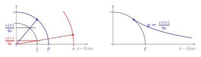
Figure 5: The set $\partial G$ in the first quadrant.

We must observe that $\partial G$ is symmetric with respect the $x$-axis and $y$-axis. Therefore, $\partial G$ is completely determined by the points in the curve solution to $|y|=\frac{r\epsilon(r)}{q_{0}}$ contained in the first quadrant, see Figure 6.

Figure 6: The set $G$.

We have obtained that the set $G$ is bounded by two curves $L^{+}$ and $L^{-}$. The curve $L^{-}$ is the union of the curves solution to $|y|=\frac{r\epsilon(r)}{q_{0}}$ in the first and the second quadrants and the arc of $\partial B(\bar{r})$ (in these quadrants) joining these curves. This arc can be described as the set of points $(x,y)\in\partial B(\bar{r})$ such that $y\geq\frac{\bar{r}\epsilon(\bar{r})}{q_{0}}$, see the left side of Figure 5 . The curve $L^{+}$ is the reflection of $L^{-}$ with respect to the $x-$axis. A sketch of the set $G$ is presented in the Figure 6.

On the one hand, any $(x,y)\in L^{-}$ satisfies either $y=\frac{r\epsilon(r)}{q_{0}}$ or $y\geq\frac{\bar{r}\epsilon(\bar{r})}{q_{0}}$. Therefore on $L^{-}$ either $\psi(x,y)=\phi(x,y)-q_{0}y=\phi(x,y)-r\epsilon(r)<0$ or $|(x,y)|=\bar{r}$ and $\psi(x,y)=\phi(x,y)-q_{0}y\leq\phi(x,y)-\bar{r}\epsilon(\bar{r})<0$. Thus, the function $\psi$ is negative on $L^{-}$. Analogously we can prove that $\psi$ is positive on $L^{+}$. On the other hand, any point $(x,y)$ above the curve $L^{-}$ satisfies $y>\frac{r\epsilon(r)}{q_{0}}$, then we can conclude that $\psi(x,y)=\phi(x,y)-q_{0}y<r\epsilon(r)-r\epsilon(r)=0$. In the same way, any point $(x,y)$ below the curve $L^{+}$ satisfies $\psi(x,y)>0$.

This shows that the set $\{(x,y)\in\mathbb{R}^{2}\setminus B:\psi(x,y)=0\}$ must be strictly contained in $G$. Clearly this set is not empty since $\psi$ alternates between $-m(\gamma_{0})$ and $m(\gamma_{0})$ on $\partial B(r_{0})$. Let us denote the sets

$$\Omega^{+} = \{(x,y)\in\mathbb{R}^{2}\setminus B(r_{0}):\psi(x,y)>m(\gamma_{0})\},$$

$$\Omega^{-} = \{(x,y)\in\mathbb{R}^{2}\setminus B(r_{0}):\psi(x,y)<-m(\gamma_{0})\}.$$

Claim B.

Neither $\Omega^{+}$ nor $\Omega^{-}$ is empty.

Proof of Claim B.

Suppose that the set $\Omega^{+}$ is empty; then $\psi(x,y)\leq m(\gamma_{0})$ for all $(x,y)\in\mathbb{R}^{2}\setminus B(r_{0})$. Recalling that $\psi(x,y)=\phi(x,y)-q_{0}y$ we infer that $\phi(x,y)\leq q_{0}y+m(\gamma_{0})$, this means that the end $E$ is placed below the plane $q_{0}y+m(\gamma_{0})$ which is above the plane parallel to $P_{\gamma_{0}}$ at distance $m(\gamma_{0})$, see Figure 7. The intersection between the end and the plane has no interior points of the end, by the geometric comparison principle. Consequently, the intersection occurs only on $\partial B(\bar{r})$ and this intersection is transversal, again by the geometric comparison principle. Moreover, as $r\to\infty$, the distance between the end $E$ and the plane $q_{0}y+m(\gamma_{0})$ goes to infinity since the function $\phi$ has sublinear growth and the Gauss map goes to $\nu$ at infinity. Now we can decrease the inclination of the plane keeping the end $E$ below until we obtain either an interior first contact point between the end and some plane, or a horizontal plane such that $E$ is below of this plane, see Figure 8. The first case cannot happen, by the geometric comparison principle, and the second case contradicts the assumption (15). Analogously, the statement $\Omega^{-}=\varnothing$ contradicts that $E$ grows also infinitely in the direction $-\nu$. This proves Claim B. ∎

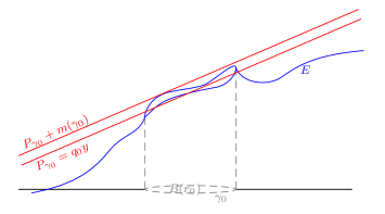
Figure 7: Assuming that $\Omega^{+}$ is empty.

Figure 8: Decreasing the inclination of the plane.

Claim C.

Each component of $\Omega^{+}$ and $\Omega^{-}$ is unbounded.

Proof of Claim C.

Suppose that a component of $\Omega^{+}$ is bounded; geometrically this means that the part of the end $E$, corresponding to that component, above the plane $q_{0}y+m(\gamma_{0})$ is compact. Hence for a positive constant $c$ the plane $q_{0}y+m(\gamma_{0})+c$ and the end $E$ have an interior contact point, again the geometric comparison principle leads to a contradiction. Analogously for the components of $\Omega^{-}$. This proves Claim C. ∎

Claim D.

Each set $\Omega^{+}$ and $\Omega^{-}$ has at least two connected unbounded components.

Proof of Claim D.

Each component of the sets $\Omega^{+}$ and $\Omega^{-}$ is unbounded by Claim C. Note that $\beta_{1}^{+},\beta_{2}^{+}\in\overline{\Omega^{+}}$ and $\beta_{1}^{-},\beta_{2}^{-}\in\overline{\Omega^{-}}$. Let us denote by $\Omega_{i}^{\pm}$ the connected component of $\Omega^{\pm}$ such that $\beta_{i}^{\pm}\in\partial\Omega_{i}^{\pm}$. Assume $\Omega_{1}^{+}=\Omega_{2}^{+}$, then we can connect the points $\beta_{1}^{+}$ and $\beta_{2}^{+}$ by a curve contained in $\Omega_{1}^{+}=\Omega_{2}^{+}$, moreover, we can connect these points also by a line segment contained in $B(r_{0})$; these curves enclose a compact set containing either $\beta_{1}^{-}$ or $\beta_{2}^{-}$, hence one of the sets $\Omega_{i}^{-}$ is contained in this compact set, thus $\Omega_{i}^{-}$ is empty, since all components are unbounded, see Figure 9. Interchanging the roles of $\Omega_{i}^{+}$ and $\Omega_{i}^{-}$, we obtain a similar conclusion. Then, it is enough to prove that all the sets $\Omega_{i}^{\pm}$ are not empty. Suppose that $\Omega_{1}^{+}=\varnothing$. In this case, the end $E$, in a neighborhood of $\phi(\beta_{1}^{+})$, is below the plane $q_{0}y+m(\gamma_{0})$. This situation is avoided by the geometric comparison principle. The same argument is valid for the other sets. This proves Claim D. ∎

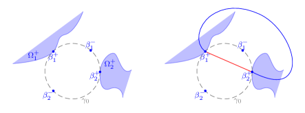
Figure 9: Assuming that $\Omega_{1}^{+}=\Omega_{2}^{+}$.

Now we will consider the components of the sets

$$\left\{(x,y)\in\mathbb{R}^{2}\setminus B(r_{0}):\psi(x,y)>0\right\}\quad\mbox{and}\quad\left\{(x,y)\in\mathbb{R}^{2}\setminus B(r_{0}):\psi(x,y)<0\right\}.$$

Each of these sets have at least two components containing the sets $\Omega_{i}^{\pm}$. We will denote these components as ${\Omega^{\prime}}_{i}^{\pm}$, then

$$\beta_{i}^{+}\in\overline{\Omega_{i}^{+}}\subset{\Omega^{\prime}}_{i}^{+}\mbox{ \ and \ }\beta_{i}^{-}\in\overline{\Omega_{i}^{-}}\subset{\Omega^{\prime}}_{i}^{-}.$$

Claim E.

Each set ${\Omega^{\prime}}_{i}^{\pm}$ contains a Jordan curve $J_{i}^{\pm}(t)=(x_{i}^{\pm}(t),y_{i}^{\pm}(t))$ contained in the set $\overline{G}\setminus B(r_{0})$ such that $x_{i}^{+}(t)\to\infty$ as $t\to\infty$ and $x_{i}^{-}(t)\to-\infty$ as $t\to\infty$.

Proof of Claim E.

If any of the sets ${\Omega^{\prime}}_{i}^{\pm}$ contains a point of $L^{\pm}$, then by the connectedness it must contain the whole curve $L^{\pm}$. In this case the curve $L^{\pm}$ satisfies the condition required.

Now suppose that some set ${\Omega^{\prime}}_{i}^{\pm}$ does not touch the curve $L^{\pm}$, this implies that ${\Omega^{\prime}}_{i}^{\pm}\subset\overline{G}\setminus B(r_{0})$. We now add the points $+\infty$ and $-\infty$ to the boundary of $G$ and consider again the set $\Omega_{i}^{\pm}$, then clearly $\partial G\cap\partial\Omega_{i}^{\pm}\subset\{-\infty,+\infty\}$. Assume that $+\infty$ is not in the common boundary, thereby there exists a large enough positive constant $C$ such that $\Omega_{i}^{\pm}\subset\left\{(x,y)\in\mathbb{R}^{2}:x\leq C\right\}$. In this case we can easily find an angle less than $\pi$ where the set $\Omega_{i}^{\pm}$ can be placed, since $\frac{\epsilon(r)}{q_{0}}\to 0$ as $r\to\infty$; Figure 10 shows how to build the angle sector.

Applying Lemma 7 to the function $\psi-m(\gamma_{0})$ on the set $\Omega_{i}^{\pm}$, we obtain that for $r$ big enough and some $(x,y)$ with $|(x,y)|=r$ we have

$$\psi(x,y)-m(\gamma_{0})>cr.$$

However, $\phi$ has sublinear growth on $\Omega_{i}^{\pm}$, i.e.,

$$\psi(x,y)-m(\gamma_{0}) =\phi(x,y)-q_{0}y-m(\gamma_{0})$$

$$\leq r\epsilon(r)+q_{0}|y|-m(\gamma_{0})$$

$$\leq 2r\epsilon(r)-m(\gamma_{0}),$$

but the above inequalities imply that $\epsilon(r)>\frac{c}{2}$, which is a contradiction since $\epsilon(r)\to 0$ as $r\to\infty$.

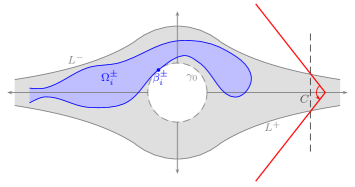
Figure 10: The set $\Omega_{i}^{\pm}$ placed in an angle sector.

Summarizing, we have proven that $\partial G\cap\partial\Omega_{i}^{\pm}=\{-\infty,+\infty\}$ for all sets $\Omega_{i}^{\pm}$; therefore Lemma 8 guaranties the existence of the Jordan curves $J_{i}^{\pm}$. This proves Claim E. ∎

To finish the proof of the growth lemma, consider for $i=1,2$ a curve in $G$ that joins $+\infty$ and $\beta_{i}^{+}$, also consider the segment inside $B(r_{0})$ joining $\beta_{1}^{+}$ and $\beta_{2}^{+}$. The closed curve formed by these three curves must enclose one of the points $\beta_{i}^{-}$, and, in consequence, they must enclose one of the sets $\Omega_{i}^{-}$. This is a contradiction because now $-\infty$ is not accessible from within $\Omega_{i}^{-}$, see Figure 11. This concludes the proof of the lemma.

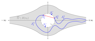
Figure 11: The point $\beta_{2}^{-}$ cannot be connected to $-\infty$ by the curve $J_{2}^{-}$.

∎

As a consequence of the growth lemma we have an obstruction for non-planar one ended ESWMT-surfaces with finite total curvature in $\mathbb{R}^{3}$. This is an evidence about the premise that the theory of ESWMT-surfaces is quite similar to the theory of minimal surfaces, even more if we note that there is not such obstruction for harmonic surfaces of finite total curvature, see [14].

Theorem 9.

Let $\Sigma\subset\mathbb{R}^{3}$ be a complete connected ESWMT-surface satisfying (1) of finite total curvature and one embedded end. Then $\Sigma$ is a plane.

Proof.

Since $\Sigma$ has finite total curvature, Lemma 2 says that $\Sigma$ has finite total second fundamental form. Then, Theorem 8 and the growth lemma (Lemma 4) imply that $\Sigma$ lies in a half-space of $\mathbb{R}^{3}$. Thus, by the half-space theorem, Corollary 1, $\Sigma$ is a plane. ∎

2.2 Logarithmic growth

The second claim about the height function $u:\mathbb{D}^{*}\rightarrow\mathbb{R}$ of an embedded ESWMT-end $E$ satisfying (1) of finite total curvature is that this function is asymptotically radial as $|z|\to 0^{+}$ and has logarithmic growth.

The function $u$ satisfies the Poisson equation (13), which can be written as $\Delta u=2\lambda\theta f(q)$ provided the Weingarten relation $H=f(q)$. Henceforth, we will consider that $u\geq 0$, hence $u$ and $\Delta u$ have the same sign, by the growth lemma and the conditions (1). Note that the case of $u\leq 0$ is completely analogous since we can redefine $\nu$ as $-\nu$, this will change the sign of the angle function $\theta$ and we will have the same conclusion.

In a neighborhood of $0$ we obtain that

$$\Delta u=2\lambda\theta f(q)\leq 4\delta\lambda\theta q=\delta\lambda\theta(|II|^{2}-2K),$$ (16)

for some positive constant $\delta$.

Recalling that $\theta\leq 1$, Lemma 2 and integrating around the origin, we conclude, redefining the end $E$ if necessary, that

$$\int_{\mathbb{D}^{*}}\Delta u\,|dz|^{2}\leq\delta\int_{\mathbb{D}^{*}}\lambda(|II|^{2}-2K)\,|dz|^{2}=\delta\int_{E}(|II|^{2}-2K)\,dA<\infty.$$ (17)

The desired conclusions about the function $u$ are obtained from (16), (17) and the next Lemma.

Lemma 9 (S. Taliaferro, [49]).

Let $u$ and $\varphi$ be non-negative functions defined on $\mathbb{D}^{*}$, such that $\Delta u=\varphi$ in $\mathbb{D}^{*}$ and $\varphi$ is integrable over the whole disk $\mathbb{D}$. Then, there exists a constant $\beta$ and some continuous function $u_{h}:\mathbb{D}\rightarrow\mathbb{R}$, which is harmonic in $\mathbb{D}$, such that for any $z\in\mathbb{D}^{*}$ we have

$$u(z)=\beta\log|z|+u_{h}(z)+u_{N}(z),$$ (18)

where the function $u_{N}$ is the Newtonian potential of $\varphi$ and is defined by

$$u_{N}(z)=\frac{1}{2\pi}\int_{\mathbb{D}}\log\frac{1}{|z-\xi|}\varphi(\xi)\,|d\xi|^{2}.$$ (19)

The behavior of the Newtonian potential of $\varphi$ near the singularity can be described as follow.

Lemma 10 (S. Taliaferro, [51]).

Let $u$ and $\varphi$ as in Lemma 9. If there exists a non-negative constant $C$ and $0<r\leq 1$ such that $\varphi(z)\leq(2|z|)^{-C}$ for $z\in\mathbb{D}(r)^{*}$, then the Newtonian potential of $\varphi$ satisfies

$$u_{N}(z)=o\left(\log\frac{1}{|z|}\right)\mbox{ \ as \ }|z|\to 0.$$ (20)

As we have pointed out above in Lemma 2, the mean curvature $H$ goes to $0$ as $|z|\to 0$. Then given a non-negative constant $C$ and a positive constant $A$, for $|z|$ small enough, we can assume that $H(z)\leq 2^{-C+1}A^{-1}$. Therefore, by recalling that the angle function is bounded above by $1$, from (13) we get

$$\Delta u\leq\frac{1}{2^{C}A}\lambda,$$ (21)

where $\lambda$ is the conformal factor of the metric.

Now, in order to estimate $\lambda$, we have the following theorem that is an easy consequence of several theorems proven by R. Finn, see [17, 18].

Theorem 10 (R. Finn, [18]).

Let $\Sigma$ be a complete Riemannian surface of finite total curvature in a neighborhood $E$ of one of its ideal boundary components. Suppose that the region of positive curvature has compact support on the surface. Then $E$ can be mapped conformally onto the punctured disk $\mathbb{D}^{*}$ in the complex plane. Let denote by $\lambda|dz|^{2}$ the conformal metric. Then there exist constants $A$ and $\Phi_{0}$ such that $\lambda(z)\leq A|z|^{-2\Phi_{0}}$ as $|z|\to 0$. Moreover $\Phi_{0}\geq-1$.

Therefore, using last theorem and (21), we conclude that for $|z|$ small enough $\Delta u\leq(2|z|)^{-C}$, where $C=\max\{0,2\Phi_{0}\}$. This allows us to use Lemma 10 in our geometric context and infer that

$$\lim_{|z|\to 0^{+}}\frac{u(z)}{\log|z|}=\beta.$$ (22)

2.2.1 The Beltrami equation and quasiconformal maps

The Gauss map $g$ of an immersed surface in $\mathbb{R}^{3}$ satisfies a very rich partial differential equation, the Beltrami equation. In general this equation can be written as

$$g_{\bar{z}}=\mu g_{z}.$$ (23)

Although there is a variety of equivalent definitions for a quasiconformal map, here we will consider the definition based on the Beltrami equation. This definition is taken from [19, p. 47].

Definition 1.

Let $D\subset\mathbb{C}$ be a domain. The function $g:D\rightarrow\mathbb{C}$ is called a quasiconformal map if it is a homeomorphic solution of the Beltrami equation (23) with $||\mu||_{\infty}<1$.

Given a quasiconformal map $g$, at points $z\in D$ where $g$ is differentiable we define the value

$$\Gamma_{\mu}(z)=\frac{1+|\mu(z)|}{1-|\mu(z)|}=\lim_{r\to 0^{+}}\frac{\underset{|w-z|=r}{\max}\,|g(z)-g(w)|}{\underset{|w-z|=r}{\min}\,|g(z)-g(w)|}.$$

This value is called the dilatation of $g$ at $z$. The maximal dilatation of $g$ is defined as $\Gamma_{g}=\underset{z\in D}{\sup}\,\Gamma_{\mu}(z)$ and it satisfies

$$\Gamma_{g}=\frac{1+||\mu||_{\infty}}{1-||\mu||_{\infty}}.$$ (24)

It is very common to find the notation $\Gamma_{g}$-quasiconformal to indicate a quasiconformal map $g$ with maximal dilatation $\Gamma_{g}$ or parameter of quasiconformality $\Gamma_{g}$, see for example [2].

Note that $1$-quasiconformal maps are exactly the conformal maps because $\Gamma_{g}=1$ only when $\mu=0$ which means, from the Beltrami equation, that $g_{\bar{z}}=0$, i.e., $g$ is holomorphic. This is precisely what happens when the function $g$ is the Gauss map of a minimal immersion. In this case we say that $g$ is antiholomorphic since we usually construct $g$ by sterographic projection from $(0,0,1)$.

A posthumous paper by A. Mori [37] studies quasiconformal maps from the unit ball into itself such that the origin is fixed. The main result of this paper is known nowadays as the Mori theorem and it establishes a Hölder condition for the function $g$.

Theorem 11 (Mori theorem).

Let $g:\mathbb{D}\rightarrow\mathbb{D}$ be a $\Gamma_{g}$-quasiconformal map with $g(0)=0$. Then

$$|g(z)-g(w)|\leq 16|z-w|^{1/\Gamma_{g}},$$ (25)

for all $z,w\in\mathbb{D}$. Furthermore, the constant $16$ in (25) cannot be replaced by any smaller constant independent of $\Gamma_{g}$.

Let us go back to our geometric context, where $g$ is the Gauss map of an ESWMT-surface of finite total curvature. According to Theorem 6, the Gauss map satisfies the Beltrami equation with $\mu=\frac{H\lambda}{Q}$. Using the Weingarten relation $H=f(q)$ we conclude that

$$|\mu|=\frac{f(q)}{\sqrt{q}}.$$

We can assert, since $f$ is Lipschitz at $t=0$, that

$$\limsup_{t\to 0^{+}}\frac{f(t)}{\sqrt{t}}=0,$$ (26)

hence, since $q\to 0$ at infinity, $||\mu||_{\infty}\leq\sigma<1$; for some non-negative constant $\sigma$.

Summarizing, we have proven the Gauss map of an embedded ESWMT-end satisfying (1) is a $\Gamma_{g}$-quasiconformal map, where the parameter of quasiconformality satisfies

$$\Gamma_{g}\leq\frac{1+\sigma}{1-\sigma}.$$

In order to use Mori’s theorem, we are going to distinguish for a moment between the Gauss map obtained by the stereographic projection from $(0,0,-1)$ and $(0,0,1)$ writing $g$ for the first case (as it was being) and $\varrho$ for the second one. Then we have that $\varrho(0)=0$ and, by Mori’s theorem, $\varrho$ satisfies for all $z\in\mathbb{D}$ that

$$|\varrho(z)|\leq 16|z|^{\frac{1-\sigma}{1+\sigma}}.$$

This means that $\varrho(z)=O\left(|z|^{\epsilon}\right)$ as $|z|\to 0$, where $1\geq\epsilon=\frac{1-\sigma}{1+\sigma}>0$. Since $g\bar{\varrho}=1$ we deduce that

$$g(z)=O\left(|z|^{-\epsilon}\right)\mbox{ as }|z|\to 0.$$ (27)

Redefining the end $E(r)\subset E$; we can parametrize conformally as $\mathbb{D}^{*}(r)$, for $0<r<1$. Observe that, from (26), we have

$${\rm sup}\left\{\left|\mu\right|\,:\,\,\mathbb{D}^{*}(r)\right\}\to 0\text{ as }r\to 0^{+}.$$

Then, following the computations above, the parameter of quasiconformality in $\mathbb{D}^{*}(r)$, denoted by $\Gamma_{g}(r)$, satisfies

$$\Gamma_{g}(r)\to 1\text{ as }r\to 0^{+},$$

therefore, (27) can be rewritten as

$$g(z)=O\left(|z|^{-1}\right)\mbox{ as }|z|\to 0.$$ (28)

2.2.2 Regularity at infinity for ESWMT-surfaces

Let $E$ be an embedded end of an ESWMT-surface satisfying (1) of finite total curvature. According to Theorem 8, $E$ can be described as a graph of a real valued function $\phi$ defined on the complement of a compact set in a plane, which is orthogonal to the limit of the Gauss map at infinity. We would like to understand the asymptotic behaviour of this function as in the case of minimal surfaces [47]. Until now, we have described the end $E$ by a conformal parametrization $\alpha:\mathbb{D}^{*}\rightarrow E$ such that the function $u=\langle\alpha,\nu\rangle$ is determined by (18) and satisfies $u(z)=O\left(\log|z|\right)$ as $|z|\to 0$.

By Lemma 9 we know that the function $u_{h}$ is harmonic on $\mathbb{D}$. Using an homogeneous expansion for the function $u_{h}$ at $0\in\mathbb{D}$, see [5, p. 100], and Lemma 10, we can rewrite (18) for any $z=x+iy\in\mathbb{D}^{*}$ as

$$u(z)=\beta\log|z|+a_{0}+a_{1}x+a_{2}y+O\left(|z|^{2}\right)+o\left(\log\frac{1}{|z|}\right)\mbox{ as }|z|\to 0,$$ (29)

for some real constants $\beta,a_{0},a_{1},a_{2}$. Here, we have used that there are only two linearly independent homogeneous harmonic polynomials of degree $m$ in two dimensions, namely, the real and the imaginary part of $z^{m}$.

In order to establish an easy notation, we will assume that the Gauss map takes the value $\nu=(0,0,1)$ at infinity and the function $\phi$ is defined on the complement of a compact subset of $\mathbb{R}^{2}=\{(x_{1},x_{2},0):x_{1},x_{2}\in\mathbb{R}\}\subset\mathbb{R}^{3}$. Note that with this convention the function $u$ is the third coordinate function of $E$; naming $x_{1}$ and $x_{2}$ the other coordinates of the diffeomorphism $\alpha$ we can write $\alpha=(x_{1},x_{2},u)$. From this, it is clear that the functions $u$ and $\phi$ are essentially the same, in fact $\phi(x_{1},x_{2})=u(z(x_{1},x_{2}))$. In order to know how the parameter $z$ depends of $x_{1}$ and $x_{2}$ we will use the Kenmotsu representation, Theorem 7, to recover the coordinate functions $x_{1}$ and $x_{2}$ in terms of $z$.

From (7) we have the following equations

$$\partial_{z}x_{1}=-\frac{\bar{g}_{z}(1+g^{2})}{H(1+g\bar{g})^{2}},$$

$$\partial_{z}x_{2}=-\frac{i\bar{g}_{z}(1-g^{2})}{H(1+g\bar{g})^{2}},$$

$$\partial_{z}u=-\frac{2\bar{g}_{z}g}{H(1+g\bar{g})^{2}}.$$

Hence we conclude that $\partial_{z}(x_{1}+ix_{2})=-g\partial_{z}u$ and we can recover $x_{1}+ix_{2}$ by integration from the Kenmotsu representation.

Since $u(z)=O(\log|z|)$ as $|z|\to 0$ by (22), we have that $\partial_{z}u(z)=O\left(|z|^{-1}\right)$ as $|z|\to 0$. On the other hand, from the ellipticity of the function $f$, we have (28), i.e., $g(z)=O\left(|z|^{-1}\right)$ as $|z|\to 0^{+}$. We reach upon integration that $x_{1}+ix_{2}=O\left(|z|^{-1}\right)$ as $|z|\to 0$. Defining $r=|x_{1}+ix_{2}|$, we have that $|z|=O\big{(}r^{-1}\big{)}$ as $r\to+\infty$. Again, rewriting the function $u$, from the equation (29), we achieve the following description of the asymptotic behavior of the function $\phi$,

$$\phi(x_{1},x_{2})=\beta\log r+a_{0}+\frac{a_{1}x_{1}}{r^{2}}+\frac{a_{2}x_{2}}{r^{2}}+O\big{(}r^{-2}\big{)}+o\left(\log r\right)\mbox{ as }r\to+\infty,$$

for some real constants $\beta,a_{0},a_{1},a_{2}$ (not necessarily the same constants of (29)).

Summarizing all the results achieved in this section, we get

Theorem 12.

Let $\Sigma\subset\mathbb{R}^{3}$ be a complete ESWMT-surface satisfying (1) of finite total curvature and embedded ends. Then each end $E_{i}$ is the graph of a function $\phi_{i}$ over the exterior of a bounded region in some plane $\Pi_{i}$. Moreover, if $x_{1},x_{2}$ are the coordinates in $\Pi_{i}$, then the function $\phi_{i}$ have the following asymptotic behaviour for $r=|x_{1}+ix_{2}|$ large

$$\phi_{i}(x_{1},x_{2})=\beta\log r+a_{0}+\frac{a_{1}x_{1}}{r^{2}}+\frac{a_{2}x_{2}}{r^{2}}+O\big{(}r^{-2}\big{)}+o\left(\log r\right),$$ (30)

where $\beta,a_{0},a_{1},a_{2}$ are real constants depending on $i$.

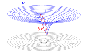
Figure 12: Representation of an end $E$ of an ESWMT-surface satisfying the hypothesis of Theorem 12.

Theorem 12 implies that, if the planes $\Pi_{\nu_{i}}$ are not parallel, then the ends must intersect. In particular, when the surface $\Sigma$ is embedded outside a compact set and has two ends, we have that these ends can be described as graphs of functions defined over the same plane $\Pi$. Moreover, the surface $\Sigma$ must grow infinitely in both sides of the plane $\Pi$, since it cannot be contained in a half-space by the half-space theorem, Corollary 1. Recall that the vectors $\nu_{i}$ are the continuous extension of the Gauss map to the ideal boundary $\{p_{i}\}$, Theorem 8. When the vectors $\nu_{i}$ are parallel, we will say that the corresponding ends $E_{i}$ are parallel.

We summarize this fact in the next lemma.

Lemma 11.

Let $\Sigma\subset\mathbb{R}^{3}$ be a complete ESWMT-surface satisfying (1) of finite total curvature embedded outside a compact set and two ends. Then, the ends of $\Sigma$ are parallel and the surface must grow infinitely in opposite directions.

We would like to finish this section by noting that the equality (30) can be seen as a generalization of the concept of regular at infinity given by Schoen in [47].

3 Jorge-Meeks type formula

Here, we will extend the famous Jorge-Meeks formula for complete minimal surfaces of finite total curvature. In fact, we will give first a proof by using the Simons formula for minimal surfaces. As far as we know, this approach was not known:

Theorem 13 (Jorge-Meeks formula).

Let $\Sigma\subset\mathbb{R}^{3}$ be a complete minimal surface of finite total curvature of genus $g$ and $k$ embedded ends, then

$$\int_{\Sigma}K\,dA=4\pi(1-g-k).$$

Proof.

Since $\Sigma$ has finite total curvature, it is conformally equivalent to a compact surface of genus $g$, $\Sigma_{g}$, with $k$ points removed.

Let $D_{i}^{*}(r)$, $i=1,\ldots,k$, be punctured conformal disks pairwise disjoint corresponding to the ends. Since the ends are embedded, the first fundamental form is asymptotic to $c_{i}|z-p_{i}|^{-4}|dz|^{2}$, where $z$ is a complex coordinate in $D_{i}^{*}(r)$ and $c_{i}$ is a positive constant. The positive constant $c_{i}$ can be computed as

$$\lim_{r\to 0}r^{2}\,A\left(D_{i}(r_{0})\setminus\overline{D_{i}(r)}\right)=\pi c_{i};$$ (31)

where $A(\Omega)$ denote the area of $\Omega\subset\Sigma$ measured with respect to $I$.

Let $Q$ be the Hopf differential, since $K\to 0$ as $p\to p_{i}$, then $Q(p_{i})=0$ for all $i=1,\ldots,k$; observe here that the Hopf differential extends meromorphically to the ends.

The umbilic points are isolated and $K<0$ on each $D_{i}$ hence, there is only a finite number, $\{x_{1},\ldots,x_{m}\}$, of umbilic points at the interior. Consider $D_{j}(r)$, $j=1,\ldots,m$, geodesic disks of radius $r$ centered at $x_{j}$, $j=1,\ldots,m$, pairwise disjoints.

Set $\Sigma_{r}=\Sigma\setminus\bigcup_{i=1}^{k}D_{i}(r)^{*}\cup\bigcup_{j=1}^{m}D_{j}(r)$; then the Simons formula reads as

$$\Delta\ln|II|=2K\text{ in }\Sigma_{r},$$

then, integrating in both sides of the above equality and using the divergence theorem we get

$$2\int_{\Sigma_{r}}K\,dA=\sum_{i=1}^{k}\int_{\partial D^{*}_{i}(r)}\langle\nabla\ln|II|,\nu\rangle\,dA+\sum_{j=1}^{m}\int_{\partial D_{j}(r)}\langle\nabla\ln|II|,\nu\rangle\,dA,$$

where $\nu$ is the inward normal along either $D_{i}^{*}(r)$ or $D_{j}(r)$.

Consider $z$ a local conformal parameter on $D_{j}(r)$, then we can write $|II|=|Q|/\lambda$, where $I=\lambda|dz|^{2}$. Since the conformal factor $\lambda$ is regular at $x_{j}$, $j=1,\ldots,m$, then

$$\int_{D_{j}(r)}\langle\nabla\ln|II|,\nu\rangle\,dA\to-2\pi{Ord}_{x_{j}}Q\text{ as }r\to 0,$$

where ${Ord}_{x_{j}}Q$ is the order of the zero (or pole) of the Hopf differential at $x_{j}$.

Consider $z$ a local conformal parameter on $D^{*}_{i}(r)$, then we can write $|II|=|Q|/\lambda$, where $I=\lambda|dz|^{2}$. Since the conformal factor $\lambda$ is asymptotic to $c_{i}|z-p_{i}|^{-4}$ at $p_{i}$, $i=1,\ldots,k$, then

$$\int_{D^{*}_{i}(r)}\langle\nabla\ln|II|,\nu\rangle\,dA\to-2\pi{Ord}_{p_{i}}Q-8\pi\text{ as }r\to 0,$$

where ${Ord}_{p_{i}}Q$ is the order of the zero (or pole) of the Hopf differential at $p_{i}$.

By the Poincaré-Hopf index theorem the sum of the order of the zeroes and poles of the Hopf differential is $-2\chi(\Sigma_{g})=-4(1-g)$. Therefore, joining all the above information we get

$$\int_{\Sigma}K\,dA=4\pi(1-g-k),$$

as desired. ∎

Let $\Sigma\subset\mathbb{R}^{3}$ be a complete ESWMT-surface satisfying (1) of finite total curvature and embedded ends. Then, by the results described in Section 1.4, the adapted Codazzi pair $(I_{f},II_{f})$ satisfies that $I_{f}$ is a complete metric on $\Sigma$ since $q\to 0$ at infinity.

Since $\Sigma$ has finite total curvature; it is conformally equivalent with respect to the conformal structure given by the first fundamental form $I$ to a compact Riemann surface minus a finite number of punctures $p_{i}$, $i=1,\ldots,k$. Let $D_{i}^{*}(r)$ be a punctured conformal disk with respect to the conformal structure given by $I$ around $p_{i}$, consider $r>0$ small enough so that the punctured disks $D_{i}^{*}(r)$ are pairwise disjoint. From (11) and the fact that $q\to 0$ at infinity; there exists a constant $C(r)\geq 1$ so that

$$C(r)^{-1}I_{f}\leq I\leq C(r)I_{f}\text{ on }D_{i}^{*}(r),$$

where the constant $C(r)$ satisfies $C(r)\to 1$ as $r\to 0$. This means that $D_{i}^{*}(r)$ is also conformally equivalent to a punctured disk with respect to the conformal structure given by $I_{f}$; or, in other words, $I$ and $I_{f}$ are isometric at infinity. Moreover, the area element of $I$, $dA$, is pointwise equal to the area element of $I_{f}$, $dA_{f}$; the last statement is general and it follows from (11).

Also, there exists a holomorphic (with respect to the conformal structure of $I_{f}$) quadratic differential, denoted by $Q_{f}$, whose zeroes coincide with the umbilic points of $\Sigma$. Moreover, since $I$ and $I_{f}$ are isometric at infinity, the conformal factor associated to $I_{f}$ at a punctured $p_{i}$ is asymptotic to $c_{i}|z-p_{i}|^{-4}|dz|^{2}$, where $z$ is a complex coordinate in $D_{i}^{*}(r)$ with respect to the conformal structure given by $I_{f}$ around $p_{i}$, and $c_{i}$ is the positive constant given by (31); the last statement follows by the fact that the area elements, $dA$ and $dA_{f}$, coincide pointwise; that is,

$$\lim_{r\to 0}r^{2}\,A_{f}\left(D_{i}(r_{0})\setminus\overline{D_{i}(r)}\right)=\pi c_{i};$$ (32)

where $A_{f}(\Omega)$ denote the area of $\Omega\subset\Sigma$ measured with respect to $I_{f}$. Also, the quadratic differential extends meromorphically to the punctures as above.

Therefore, using the Simons type formula given in Section 1.4, integrating over $\Sigma_{r}=\Sigma\setminus\bigcup_{i=1}^{k}D_{i}(r)^{*}\cup\bigcup_{j=1}^{m}D_{j}(r)$ and following the exact same computations as above, we obtain that:

$$\int_{\Sigma}\mathcal{K}_{f}\,dA=4\pi(1-g-k).$$

Since $(\Sigma,I)$ and $(\Sigma,I_{f})$ are complete, finitely connected and their respective total curvature are finite, K. Shiohama (cf. [48, Theorem A] or [34, Proposition 1.2]) proved that

$$\int_{\Sigma}K\,dA=2\pi\left(\chi(\Sigma)-\lim_{r\to 0}\frac{r^{2}A(\Sigma_{r})}{\pi}\right),$$

and

$$\int_{\Sigma}\mathcal{K}_{f}\,dA_{f}=2\pi\left(\chi(\Sigma)-\lim_{r\to 0}\frac{r^{2}A_{f}(\Sigma_{r})}{\pi}\right),$$

where we have followed the notation above. Note that

$$\lim_{r\to 0}\frac{r^{2}A(\Sigma_{r})}{\pi}=\sum_{i=1}^{k}\lim_{r\to 0}\frac{r^{2}A\left(D_{i}(r_{0})\setminus\overline{D_{i}(r)}\right)}{\pi}=\sum_{i=1}^{k}c_{i}=\lim_{r\to 0}\frac{r^{2}A_{f}(\Sigma_{r})}{\pi},$$

then Shiohama’s formula, in our case, implies that

$$\int_{\Sigma}K\,dA=\int_{\Sigma}\mathcal{K}_{f}\,dA_{f}.$$

Hence, we have obtained a Jorge-Meeks type formula for ESWMT-surfaces. Specifically:

Theorem 14.

Let $\Sigma\subset\mathbb{R}^{3}$ be a complete ESWMT-surface satisfying (1) of finite total curvature with embedded ends. Let $g$ be the genus and $k$ the number of ends, then

$$\int_{\Sigma}K\,dA=4\pi(1-g-k).$$ (33)

Remark 9.

We shall say that there is a mistake in the formula given in [48, Theorem A]; the $2$ should be in the numerator instead of the denominator in the expression $\frac{A(t)}{2t^{2}}$. This has been corrected in [34, Proposition 1.2], it is the formula we have used here. We can verify it by taking the simple example of $\mathbb{R}^{2}$ with the flat metric.

4 Alexandrov reflection method for catenoidal type ends

A. Alexandrov [4] characterized spheres as the only closed connected surfaces embedded in $\mathbb{R}^{3}$ with constant (non-zero) mean curvature. Although this is a major theorem, the procedure introduced by Alexandrov have had a remarkable impact in the development of Differential Geometry. This technique is called the Alexandrov reflection method and it is based on the maximum principle, the classical result on the theory of second order elliptic partial differential equations, see [24, 27, 41].

Theorem 15 (Interior maximum principle).

Let $u$ be a $C^{2}(\Omega)$ function which satisfies the differential inequality $Lu\geq 0$ in the domain $\Omega$, where $L$ is a locally uniformly elliptic operator. If $u$ takes a maximum value $C$ in $\Omega$, then $u\equiv C$ in $\Omega$.

The interior maximum principle does not apply when the function $u$ attains its maximum value at the boundary of the domain $\Omega$. The following theorem, known as Hopf’s lemma, treats this case.

Theorem 16 (Boundary maximum principle).

Let $u$ be a $C^{2}(\Omega)\cap C^{0}(\overline{\Omega})$ function which satisfies the differential inequality $Lu\geq 0$ in the domain $\Omega$, where $L$ is a locally uniformly elliptic operator. Suppose that $\Omega$ satisfies the interior sphere condition and let $x_{0}\in\partial\Omega$ such that

• $u$ is of class $C^{1}$ in $x_{0}$.

• $u(x_{0})\geq u(x)$ for all $x\in\Omega$.

• $\partial_{\nu}u(x_{0})\geq 0$, where $\nu$ is the inward normal direction of $\partial\Omega$.

Then $u$ is constant.

4.1 The Alexandrov reflection method

Alexandrov’s idea to prove his theorem, roughly speaking, was to compare the surface with successive reflections of parts of the surface looking for a possible first tangency point, and finding at this time a plane of symmetry for the original surface. With the aim of applying this method later we are going to present the Alexandrov reflection method following [3, 16, 33], which is a generalization to non-compact surfaces.

Definition 2.

Let $\Sigma_{1}$ and $\Sigma_{2}$ be immersed surfaces in $\mathbb{R}^{3}$ and $p\in\Sigma_{1}\cap\Sigma_{2}$. The point $p$ is called a tangent point if $T_{p}\Sigma_{1}=T_{p}\Sigma_{2}$, and either $p$ is an interior point of both surfaces or $p\in\partial\Sigma_{1}\cap\partial\Sigma_{2}$ and the interior conormals vectors of $\partial\Sigma_{1}$ and $\partial\Sigma_{2}$ coincide at $p$.

Given a surface $\Sigma$ immersed in $\mathbb{R}^{3}$ and $p\in\Sigma$, we can describe locally the surface $\Sigma$, in a neighborhood of $p$, as a graph of a smooth function defined on its tangent plane at $p$, thinking of this linear space as an affine plane of $\mathbb{R}^{3}$ passing through $p$. That is, there exists a neighborhood $V\subset\Sigma$ of $p$, a domain $\Omega\subset T_{p}\Sigma$ and a smooth function $u:\Omega\rightarrow\mathbb{R}$ such that

$$\Sigma\cap V=\mathrm{Gr}\,(u)=\{q+u(q)N(p):q\in\Omega\},$$

where $N$ is a unit normal vector field defined on $\Sigma$. Note that $u(p)=0$. When the surface $\Sigma$ has no empty boundary and $p\in\partial\Sigma$, the function $u$ is defined on $\bar{\Omega}$, $p\in\partial\Omega$ and $u(\partial\Omega)=\partial\Sigma\cap V$.

Note that when the surfaces $\Sigma_{1}$ and $\Sigma_{2}$ have a common tangency point $p$ (at the interior or at the boundary), then locally those surfaces can be obtained as graphs (over the same plane) of functions $u_{1}$ and $u_{2}$ respectively, defined on the same domain ($\Omega$ or $\bar{\Omega}$ according if either $p$ is an interior or a boundary point respectively).

Let us denote by $\Sigma_{1}\geq_{p}\Sigma_{2}$ if $\Sigma_{1}$ and $\Sigma_{2}$ have the point $p$ as a common tangency point and $u_{1}\geq u_{2}$ in a neighborhood of $p$ in $\Omega$ (or $\bar{\Omega}$), which means geometrically that locally the surface $\Sigma_{1}$ is above the surface $\Sigma_{2}$ around $p$.

Now we state a geometric maximum principle using the functions that locally describe the surfaces.

Definition 3.

Let $\Sigma_{1}$ and $\Sigma_{2}$ be surfaces immersed in $\mathbb{R}^{3}$. We say that the surfaces satisfy the maximum principle if, for every common tangent point $p\in\Sigma_{1}\cap\Sigma_{2}$, the function $w=u_{2}-u_{1}$ satisfies a differential inequality $Lw\geq 0$ for some locally uniformly elliptic second order partial differential operator $L$ and, in addition, the conditions in the hypothesis of Theorem 16 when the tangent point is at the common boundary of the surfaces. Here $u_{i}$ is the function such that $\Sigma_{i}$ is locally, around $p$, represented as the graph of $u_{i}$, for $i=1,2$.

The intention of the last definition is to apply Theorem 15 and Theorem 16 thinking just in the geometric fact that two surfaces are touching tangentially to each other. Hence, using Definition 3 and the theorems mentioned we obtain the following geometric comparison principle:

Theorem 17 (Geometric comparison principle).

Let $\Sigma_{1}$ and $\Sigma_{2}$ be surfaces immersed in $\mathbb{R}^{3}$ satisfying the maximum principle. If $\Sigma_{1}\geq_{p}\Sigma_{2}$ then $\Sigma_{1}=\Sigma_{2}$ locally around $p$.

It is common to work with families of surfaces satisfying the maximum principle, see for example [3, 16].

Definition 4.

Let $\mathfrak{F}$ be a family of oriented immersed surfaces in $\mathbb{R}^{3}$. We say that $\mathfrak{F}$ satisfies the maximum principle if the following properties are fulfilled:

1. $\mathfrak{F}$ is invariant under isometries of $\mathbb{R}^{3}$.

2. If $\Sigma\in\mathfrak{F}$ and $\widetilde{\Sigma}$ is another surface contained in $\Sigma$, then $\widetilde{\Sigma}\in\mathfrak{F}$.

3. Any two surfaces in $\mathfrak{F}$ satisfy the maximum principle, in the sense of Definition 3.

As examples of families of surfaces satisfying the maximum principle we would like to mention the family of minimal surfaces and the family of surfaces with non-zero constant mean curvature. In both cases, they achieve the conditions of Definition 4 mainly because the equation $H=c$, where $c$ is a constant ($c=0$ for the case of minimal surfaces), gives a quasilinear elliptic equation when the surface is written as a graph. Although these families come from a similar equation they are quite different; for example there are no compact minimal surfaces while the sphere of radius $\frac{1}{c}$ is the unique compact embedded surface of constant mean curvature $c$ (Alexandrov Theorem).

Let $\Sigma$ be a connected properly embedded surface in $\mathbb{R}^{3}$, then the surface divides $\mathbb{R}^{3}$ into two connected components. Let us denote by $N$ a unit normal vector field globally defined on $\Sigma$. Set $\mathcal{C}(N)$ the component of $\mathbb{R}^{3}\setminus\Sigma$ pointed by $N$. Note that $\partial\mathcal{C}(N)=\Sigma$.

Consider a fixed plane $\mathcal{P}\subset\mathbb{R}^{3}$ with normal unit vector $n$. For $t\in\mathbb{R}$ we will denote by $\mathcal{P}_{t}$ the parallel plane to $\mathcal{P}$ at signed distance $t$, that is, $\mathcal{P}_{t}=\mathcal{P}+tn$. Hence, the family $\{\mathcal{P}_{t}\}_{t\in\mathbb{R}}$ is a foliation of $\mathbb{R}^{3}$ by parallel planes to $\mathcal{P}$. Set $\mathcal{P}_{t^{-}}$ and $\mathcal{P}_{t^{+}}$ the closed half spaces, lower and upper respectively, from the plane $\mathcal{P}_{t}$, i.e.,

$$\mathcal{P}_{t^{-}}=\underset{s\leq t}{\bigcup}\mathcal{P}_{s}\quad\mbox{and}\quad\mathcal{P}_{t^{+}}=\underset{s\geq t}{\bigcup}\mathcal{P}_{s}.$$

For any set $G\subset\mathbb{R}^{3}$, let $G_{t^{+}}$ be the portion of $G$ above the plane $\mathcal{P}_{t}$ and let $G_{t^{+}}^{*}$ be the reflection of this portion through the plane $\mathcal{P}_{t}$, then we can write

$$G_{t^{+}}=G\cap\mathcal{P}_{t^{+}}\quad\mbox{and}\quad G_{t^{+}}^{*}=\{p+(t-r)n:p\in\mathcal{P},\,p+(t+r)n\in G\}.$$ (34)

We define analogously the sets $G_{t^{-}}$ and $G_{t^{-}}^{*}$.

Given an open set $W\subset\mathcal{C}(N)$ consider the portion $S$ of the surface $\Sigma$ obtained by $S=\partial W\cap\Sigma$. If the set $S_{t^{+}}$ is not empty and $S_{t^{+}}^{*}\subset\bar{W}$ we write $S_{t^{+}}^{*}\geq S_{t^{-}}$, which means that the reflection of the set $S_{t^{+}}$ thought the plane $\mathcal{P}_{t}$ is above the set $S_{t^{-}}$, considering the height from the plane $\mathcal{P}$.

When $S$ is not empty, we will define a function $\Lambda_{1}$, called Alexandrov function associated to $S$.

We start with the definition of the domain of the function $\Lambda_{1}$. Given a point $p\in\mathcal{P}$, set $L_{p}$ the perpendicular line to $\mathcal{P}$ passing through $p$, therefore we can parametrize this line as $L_{p}=\{p+tn:t\in\mathbb{R}\}$. Suppose that $L_{p}\cap\bar{W}\neq\emptyset$ but $L_{p}$ is disjoint from $\bar{W}$ for all sufficiently large $t$, that is, there exists a value $t_{1}(p)$ such that $p+tn\notin\bar{W}$ for any $t>t_{1}(p)$ and $\mathbf{P}_{1}(p)=p+t_{1}(p)n\in\bar{W}$. We say that $\mathbf{P}_{1}(p)$ is the first point of contact of the set $L_{p}\cap\bar{W}$ as $t$ decreases from $+\infty$. Now we are going to suppose additionally that $\mathbf{P}_{1}(p)\in S$, then the intersection of $L_{p}$ and $S$ can be either tangential or else transversal. In the first case we will denote $\mathbf{P}_{2}(p)=\mathbf{P}_{1}(p)$ and $t_{2}(p)=t_{1}(p)$. When the intersection is transversal, we are going to look for the next point where $L_{p}$ tries to leave $\bar{W}$, if exists, that is, we look for a point $\mathbf{P}_{2}(p)=p+t_{2}(p)n$ such that $p+tn\in\bar{W}$ for any $t_{1}(p)\geq t\geq t_{2}(p)$ and $\mathbf{P}_{2}(p)\in S$. We say that $\mathbf{P}_{2}(p)$ is the second point of contact of the set $L_{p}\cap\bar{W}$ as $t$ decreases from $+\infty$.

Let us denote by $\mathcal{D}$ the domain of the Alexandrov function associated to $S$ and define it as the set of points $p\in\mathcal{P}$ such that either there exists just a first contact point or there exist the first and second contact points of the set $L_{p}\cap\bar{W}$ as $t$ decreases from $+\infty$, and those points belongs to $S$. Geometrically, $\mathcal{D}$ contains all points $p$ in the plane $\mathcal{P}$ such that the lines $L_{p}$, coming from infinity, enter $\bar{W}$ through $S$ either tangentially or transversally and leaving $\bar{W}$ also through $S$.

We define $\Lambda_{1}:\mathcal{D}\rightarrow\{-\infty\}\cup\mathbb{R}$ the Alexandrov function associated to $S$ by

$$\Lambda_{1}(p)=\left\{\begin{array}[]{cl}\dfrac{t_{1}(p)+t_{2}(p)}{2},&\mbox{if there exist }\mathbf{P}_{1}(p)\mbox{ and }\mathbf{P}_{2}(p),\\ -\infty,&\mbox{if there exists just }\mathbf{P}_{1}(p).\end{array}\right.$$ (35)

When $\Lambda_{1}$ is finite, note that $\Lambda_{1}(p)$ is the value such that the reflection of the point $\mathbf{P}_{1}(p)$ through the plane $\mathcal{P}_{\Lambda_{1}(p)}$ is $\mathbf{P}_{2}(p)$. When $\Lambda_{1}(p)=-\infty$, the reflection of $\mathbf{P}_{1}(p)$ through the plane $\mathcal{P}_{t}$, for all $t<t_{1}(p)$, is contained in $W$.

Definition 5.

A point $p\in\mathcal{D}$ is called a local interior maximum for $\Lambda_{1}$ if there exists a neighborhood $U$ of $p$ in $\mathcal{P}$ such that for any $q\in U$ either $q\in\mathcal{D}$, $\mathbf{P}_{1}(q),\mathbf{P}_{2}(q)\notin\partial S$ and $\Lambda_{1}(q)\leq\Lambda_{1}(p)$, or else $L_{q}\cap\bar{W}=\emptyset$. Any other local maximum of $\Lambda_{1}$ will be called a local boundary maximum.

Definition 6.

A first local point of reflection for $S$ with respect to the plane $\mathcal{P}$ with normal $n$ is defined to be a point $\mathbf{P}_{2}(p)$ such that $p\in\mathcal{D}$ and is a local maximum of $\Lambda_{1}$, that is, there exists a neighborhood $U$ of $p$ in $\mathcal{P}$ such that $\Lambda_{1}(q)\leq\Lambda_{1}(p)$ for any $q\in U\cap\mathcal{D}$.

The above definitions are justified through the next lemma which shows that the Alexandrov reflection method can be applied to non-compact surfaces.

Lemma 12 (Alexandrov reflection method).

Let $\mathfrak{F}$ be a family that satisfies the maximum principle and $\Sigma\in\mathfrak{F}$ be a connected surface. Let $\mathcal{P}$ be a plane in $\mathbb{R}^{3}$ with normal $n$. If, relative to the subsets $S\subset\Sigma$ and $W\subset\mathcal{C}(N)$, the Alexandrov function $\Lambda_{1}$ has a local interior maximum value $t_{0}$ at $p\in\mathcal{D}$, then the plane $\mathcal{P}_{t_{0}}$ is a plane of symmetry for $\Sigma$.

Proof.

We are going to compare the surface $S$ with the reflection $S_{t_{0}^{+}}^{*}$ of $S_{t_{0}^{+}}$ through the plane $\mathcal{P}_{t_{0}}$, keeping in mind the fact that $S$ and $S_{t_{0}}^{*}$ are surfaces in $\mathfrak{F}$. Since $\Lambda_{1}(p)=t_{0}$ we get that $\mathbf{P}_{1}(p)$ reflects to $\mathbf{P}_{2}(p)$. The local maximality hypothesis implies that there exists a neighborhood $U\subset\mathcal{P}$ of $p$ such that any $q\in U$ verifies that either $q\in\mathcal{D}$, $\mathbf{P}_{1}(q),\mathbf{P}_{2}(q)\notin\partial S$ and $\Lambda_{1}(q)\leq\Lambda_{1}(p)$, or else $L_{q}\cap\bar{W}=\emptyset$. Note that in the second case we have that $L_{q}\cap S=\emptyset$, thus we can assume $q\in\mathcal{D}$. Using the definition of the Alexandrov function (35) we get

$$t_{2}(q)\leq t_{0}-(t_{1}(q)-t_{0}).$$ (36)

Looking at (34), we infer that inequality (36) means that the reflection of $\mathbf{P}_{1}(q)$ through the plane $\mathcal{P}_{t_{0}}$ lies above the point $\mathbf{P}_{2}(q)$ and then $\mathbf{P}_{1}(q)^{*}\in\bar{W}$. Summarizing, a neighborhood of $S_{t_{0}^{+}}^{*}$ containing $\mathbf{P}_{2}(p)$ is contained in $\bar{W}$.

We have shown that $S_{t_{0}}^{*}\geq_{\mathbf{P}_{2}(p)}S$ or equivalently $\Sigma_{t_{0}}^{*}\geq_{\mathbf{P}_{2}(p)}\Sigma$; in particular $\mathbf{P}_{2}(p)$ is an interior tangent point when $\mathbf{P}_{1}(p)\neq\mathbf{P}_{2}(p)$ and a boundary tangent point when $\mathbf{P}_{1}(p)=\mathbf{P}_{2}(p)$. By Theorem 17, we conclude that $\Sigma=\Sigma_{t_{0}}^{*}$, thus $\mathcal{P}_{t_{0}}$ is a plane of symmetry of $\Sigma$. ∎

The Alexandrov reflection method is very useful any time we get a local interior maximum for the Alexandrov function. Although the function $\Lambda_{1}$ is not continuous in general, it is upper semicontinuous and it will attain its supremum in any compact domain.

The next lemma shows that the Alexandrov function $\Lambda_{1}$ is upper semicontinuous with respect to planes as well as points.

Lemma 13.

Let $S$ be a closed surface and a parameter $\varepsilon\to 0$. Suppose that there exists a sequence of points $p^{\varepsilon}\to p$ and a sequence of planes $\mathcal{P}^{\varepsilon}\to\mathcal{P}$ such that $p^{\varepsilon}\in\mathcal{P}^{\varepsilon}$ and $p\in\mathcal{P}$. Let $\Lambda_{1}^{\varepsilon}$ and $\Lambda_{1}$ be the corresponding Alexandrov functions. If $\Lambda_{1}^{\varepsilon}(p^{\varepsilon})$ and $\Lambda_{1}(p)$ exist, then

$$\limsup_{\varepsilon\to 0}\Lambda_{1}^{\varepsilon}(p^{\varepsilon})\leq\Lambda_{1}(p).$$ (37)

Proof.

Assuming $\Lambda_{1}^{\varepsilon}(p^{\varepsilon})$ exists for $\varepsilon\to 0$, then there is a sequence $\left(\mathbf{P}_{1}(p^{\varepsilon}),\mathbf{P}_{2}(p^{\varepsilon})\right)$ of pair of points of $S$ for $\epsilon\to 0$. Since $S$ is closed, a subsequence of this sequence converges to a pair of points of $S$, possibly identical, $(Q_{1},Q_{2})$. Note that clearly $Q_{1},Q_{2}\in L_{p}$ since $L_{p^{\varepsilon}}\to L_{p}$. We call $t_{1}$ and $t_{2}$ the height of these points above $\mathcal{P}$.

The values $t_{1}(p^{\varepsilon})$ and $t_{2}(p^{\varepsilon})$ converge to the height of $Q_{1}$ and $Q_{2}$ above $\mathcal{P}$, respectively. By definition of first and second contact points we conclude that the points $\mathbf{P}_{1}(p)$ and $\mathbf{P}_{2}(p)$ must be at least as hight as the points $Q_{1}$ and $Q_{2}$ respectively, that is, $t_{1}(p)\geq t_{1}$ and $t_{2}(p)\geq t_{2}$. Hence $\Lambda_{1}(p)\geq\frac{t_{1}+t_{2}}{2}$ and (37) is verified. ∎

As a first application of the Alexandrov reflection method on ESWMT-surfaces we have.

Theorem 18.

Let $\Sigma\subset\mathbb{R}^{3}$ be a complete ESWMT-surface satisfying (1) of finite total curvature, two ends and embedded outside a compact set. Then, $\Sigma$ is embedded and it has a plane of horizontal symmetry.

Proof.

Let ${\bf K}\subset\mathbb{R}^{3}$ be a compact set so that $\Sigma\setminus{\bf K}$ is embedded. By the results in Section 2, Lemma 4, Theorem 12 and Lemma 11, each end $E_{i}$; $i=1,2$, is a graph over some plane with logarithmic growth, even more, both ends are graphical over the same plane. Without lost of generality, we can assume that such plane is the horizontal plane $H:=\left\{x_{3}=0\right\}$.

Moreover, without lost of generality, we can assume that the growths $\beta_{i}$ given in Theorem 12 are different from zero; otherwise the half-space theorem, Corollary 1, implies that $\Sigma$ is a plane; contradicting that $\Sigma$ has two ends. Moreover, we can assume that $E_{1}\subset\left\{x_{3}>0\right\}$ and $\beta_{1}\leq\beta_{2}$.

Let $p\in\Sigma$ be the highest point in the $x_{3}-$direction so that the normal at $p$, $N(p)$, is horizontal. This point clearly exists since $N$ goes uniformly to the vertical vector $\pm e_{3}$ at infinity. Up to a vertical translation, we can assume that $p\in\Sigma\cap H$. Consider $\Sigma^{+}=\Sigma\cap\left\{x_{3}>0\right\}$, then $\Sigma^{+}$ is a multi-graph since $\langle N,e_{3}\rangle\neq 0$ on $\Sigma^{+}$ and it is a graph close to infinity by hypothesis; therefore $\Sigma^{+}$ is a graph over $H$.

Let $H(s)$ be the parallel plane to $H$ at height $s>0$; that is, $H(s):=\left\{x_{3}=s\right\}$. Define $\tilde{\Sigma}(s)$ as the reflection of $\Sigma\cap\left\{x_{3}>0\right\}$ with respect to the plane $H(s)$. Since $\beta_{1}\leq\beta$, $\tilde{\Sigma}(s)\cap\left(\Sigma\cap\left\{x_{3}<s\right\}\right)=\emptyset$ for $s$ big enough. Now, we can decrease $s$ from infinity to zero and, by the growth condition $\beta_{1}\leq\beta_{2}$, the first accident must occur at a finite point, which means that $\Sigma$ has a plane of horizontal symmetry by the maximum principle. If we achieve $s=0$, since at $p$ the normal is horizontal, again the maximum principle implies that $\Sigma$ has a plane of horizontal symmetry; that is, $\Sigma$ consists of two graphs over $H$, symmetric to each other with common boundary a closed curve in $H$. This proves the theorem. ∎

4.2 The Alexandrov function and tilted planes

In this subsection we are going to prove that, given an end $E$ of an ESWMT-surface as a graph of a function of the form (30) and an orthogonal plane $\mathcal{P}$, the maximum value of the Alexandrov function $\Lambda_{1}$ of $E$ respect to the plane $\mathcal{P}$ is achieved at $\partial E$.

Set $\nu:=\lim_{\left|y_{i}\right|\to+\infty}N(y_{i})$, for any proper sequence $y_{i}\in E$. Without loss of generality, we can assume that $\nu=(0,0,1)$ and $\partial E\subset\Pi_{\nu}:=\left\{p\in\mathbb{R}^{3}\,:\,\,\langle p,\nu\rangle=0\right\}$ since we can translate vertically the end $E$ and also redefining the end cutting off the compact part that is at one side of the plane $\Pi_{\nu}$ after the translation. Besides, we can also consider that the function $\phi$, given in Theorem 12, is non-negative, after a reflection through the plane $\Pi_{\nu}$, if necessary.

Let $W$ be the connected component of the upper half-space of $\Pi_{\nu}$ that contains on its boundary the bounded domain limited by $E\cap\Pi_{\nu}$. Consider a vertical plane $\mathcal{P}$ containing the vector $\nu=(0,0,1)$ and the height function respect to the plane $\Pi_{\nu}$ defined by $h(p)=\langle p,\nu\rangle$. We define the associated Alexandrov function $\Lambda:[0,\infty)\rightarrow\{-\infty\}\cup\mathbb{R}$ on $E$ (with respect to $\mathcal{P}$) as

$$\Lambda(\rho)=\max\,\{\Lambda_{1}(p):p\in\mathcal{D},\,h(p)=\rho\},$$ (38)

where $\mathcal{D}$ is the domain of the Alexandrov function $\Lambda_{1}$, (35), associated to $E$ (with respect to $\mathcal{P}$).

By Theorem 12, for any $\rho\geq 0$, the level set $E_{\rho}=\{q\in E:h(q)=\rho\}$ is a non-empty compact set. Then the function $\Lambda$ is finite valued, since the set $\{p\in\mathcal{D}:h(p)=\rho\}$ is non-empty and compact. This situation changes severely if we tilt the plane $\mathcal{P}$ slightly. We will study the consequences, on the associated Alexandrov function, caused by the tilting.

Let $n$ be the normal vector of the plane $\mathcal{P}$ and consider the vectors $\nu^{\varepsilon}=\nu+\varepsilon n$ and $n^{\varepsilon}=n-\varepsilon\nu$ for a small $\varepsilon>0$. Note that $\langle\nu^{\varepsilon},n^{\varepsilon}\rangle=0$. We will define the tilted planes $\Pi_{\nu^{\varepsilon}}=\{p\in\mathbb{R}^{3}:\langle p,\nu^{\varepsilon}\rangle=0\}$ and $\mathcal{P}^{\varepsilon}$ being the plane passing through the origin with normal vector $n^{\varepsilon}$. The height function from the plane $\Pi_{\nu^{\varepsilon}}$ is $h^{\varepsilon}$ defined by $h^{\varepsilon}(p)=\langle p,\nu^{\varepsilon}\rangle$. Clearly $\mathcal{P}^{\varepsilon}\to\mathcal{P}$, $\Pi_{\nu^{\varepsilon}}\to\Pi_{\nu}$, and $h^{\varepsilon}\to h$ as $\varepsilon\to 0$.

Since the end $E$ has logarithmic growth, we will obtain two important facts when $\varepsilon>0$ is small. The first one is that the height function $h^{\varepsilon}$ restricted to $\mathcal{D}^{\varepsilon}$ must attain a minimum value $h_{0}^{\varepsilon}$. The second one is that the Alexandrov function $\Lambda_{1}^{\varepsilon}$ is valued as $-\infty$ outside a non-empty compact set of $\mathcal{D}^{\varepsilon}$. More precisely:

Lemma 14.

Let $\varepsilon>0$. There exists a non-empty compact set $\Omega\subset\mathcal{P}^{\varepsilon}$ such that for any $p\in\mathcal{D}^{\varepsilon}\cap\left(\mathcal{P}^{\varepsilon}\setminus\Omega\right)$ there exists just first contact point of the set $\{p+tn^{\varepsilon}:t\in\mathbb{R}\}\cap\bar{W}$ as $t$ decreases from $+\infty$, i.e., $\Lambda_{1}^{\varepsilon}(p)=-\infty$.

Proof.

We are going to prove this lemma in the case that $n=(1,0,0)$. This is sufficient, since the expansion for the function $\phi$ in Theorem 12 is invariant under rotation of the $(x_{1},x_{2})$-coordinates. Let us consider a new coordinate system for $\mathbb{R}^{3}$ defined by

$$(y_{1},y_{2},y_{3})=(x_{1}-\varepsilon x_{3},x_{2},x_{3}+\varepsilon x_{1}).$$ (39)

Using these coordinates we get the planes $\mathcal{P}^{\varepsilon}=\{(y_{1},y_{2},y_{3})\in\mathbb{R}^{3}:y_{1}=0\}$ and $\Pi_{\nu^{\varepsilon}}=\{(y_{1},y_{2},y_{3})\in\mathbb{R}^{3}:y_{3}=0\}$. The intersection of the end $E$ with the plane parallel to $\Pi_{\nu^{\varepsilon}}$ at height $\tau>0$ is given by the curve

$$\Gamma_{\tau}=\left\{(y_{1},y_{2},\tau)\in\mathbb{R}^{3}:\phi\left(\frac{y_{1}}{1+\varepsilon^{2}}+\frac{\varepsilon\tau}{1+\varepsilon^{2}},y_{2}\right)=\frac{\tau}{1+\varepsilon^{2}}-\frac{\varepsilon y_{1}}{1+\varepsilon^{2}}\right\}.$$

Let $\Phi$ be the function defined as

$$\Phi(y_{1},y_{2})=\phi\left(\frac{y_{1}}{1+\varepsilon^{2}}+\frac{\varepsilon\tau}{1+\varepsilon^{2}},y_{2}\right)-\frac{\tau}{1+\varepsilon^{2}}+\frac{\varepsilon y_{1}}{1+\varepsilon^{2}}.$$

Hence,

$$\frac{\partial\Phi}{\partial y_{1}}(y_{1},y_{2})=\frac{1}{1+\varepsilon^{2}}\frac{\partial\phi}{\partial x_{1}}\left(x_{1},x_{2}\right)+\frac{\varepsilon}{1+\varepsilon^{2}},$$ (40)

where $(x_{1},x_{2})=\left(\frac{y_{1}}{1+\varepsilon^{2}}+\frac{\varepsilon\tau}{1+\varepsilon^{2}},y_{2}\right)$. Since $|\nabla\phi|\to 0$ as $r\to\infty$, there exists $R>0$, large enough, such that $\frac{\partial\phi}{\partial x_{1}}>-\varepsilon$ for all $r>R$. On the one hand, let $E_{R}$ be the set of points in $E$ such that $r\leq R$, i.e.,

$$E_{R}=\{(x_{1},x_{2},x_{3})\in E:r=\sqrt{x_{1}^{2}+x_{2}^{2}}\leq R\}.$$

Note that $E_{R}$ is a non-empty compact set, since it is the graph of a continuous function defined over a compact set. Let $\rho$ be the maximum value of the function $h^{\varepsilon}$ on the set $E_{R}$, then for $\tau>\rho$ we have that all points of $\Gamma_{\tau}$ satisfy $r>R$. On the other hand, without any assumption on $\tau$, if $(y_{1},y_{2},\tau)\in\Gamma_{\tau}$ satisfies $|y_{2}|>R$, then $r>R$. Summarizing, by (40), if $(y_{1},y_{2},\tau)\in\Gamma_{\tau}$ is a point satisfying either $\tau>\rho$ or $|y_{2}|>R$, then $\frac{\partial\Phi}{\partial y_{1}}(y_{1},y_{2})>0$. This means that if $\tau>\rho$, the entire curve $\Gamma_{\tau}$, in the $(y_{1},y_{2})$-plane is the graph of a function defined in the variable $y_{2}$ and, consequently, (in the $(y_{1},y_{2},y_{3})$-coordinates) for all $y_{2}\in\mathbb{R}$, the line $\{(t,y_{2},\tau)\in\mathbb{R}^{3}:t\in\mathbb{R}\}$ intersects the end $E$ exactly once. We have the same conclusion in the case that $|y_{2}|>R$, but only on the part of the curve satisfying the hypothesis. We define the non-empty compact set

$$\Omega=\{(0,y_{2},y_{3})\in\mathcal{P}^{\varepsilon}:|y_{2}|\leq R\mbox{ \ and \ }h_{0}^{\varepsilon}\leq y_{3}\leq\rho\}.$$

Thus, if $p\in\mathcal{D}^{\varepsilon}\cap\left(\mathcal{P}^{\varepsilon}\setminus\Omega\right)$, then $\Lambda_{1}^{\varepsilon}(p)=-\infty$. ∎

Let us define the sets $\mathcal{D}^{\varepsilon}_{0}=\{p\in\mathcal{D}^{\varepsilon}:h^{\varepsilon}(p)=h_{0}^{\varepsilon}\}$, $E^{\varepsilon}_{0}=\{p\in E:h^{\varepsilon}(p)\geq h^{\varepsilon}_{0}\}$ and $W^{\varepsilon}_{0}=\{p\in W:h^{\varepsilon}(p)\geq h^{\varepsilon}_{0}\}$, see Figure 13.

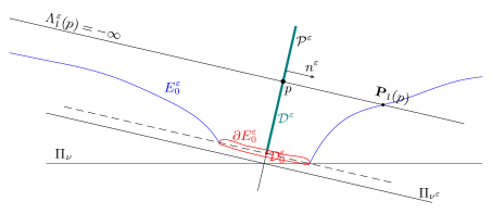
Figure 13: The Alexandrov function $\Lambda_{1}$ is valued as $-\infty$ outside of a compact set.

Lemma 15.

For the end $E$ (with all the assumptions made in this section) and any vertical plane $\mathcal{P}$ containing $\nu=(0,0,1)$, either the function $\Lambda$ is strictly decreasing, or else $\Sigma$ has a plane of reflection parallel to $\mathcal{P}$.

Proof.

We will begin proving that the function $\Lambda$ is non-increasing. For this it suffices to show that $\Lambda(\rho)\leq\Lambda(0)$ for all $\rho>0$, since we can translate vertically $E$ and redefine the end to choose the level $\rho=0$ arbitrarily.

Recall that $W=\mathcal{C}(N)\cap\{p\in\mathbb{R}^{3}:h(p)\geq 0\}$. We claim:

Claim A.

$\Lambda(\rho)\leq\Lambda(0)$ for all $\rho>0$ if, and only if,

$$E_{t^{+}}^{*}\cap\{p\in\mathbb{R}^{3}:h(p)>\rho\}\subset\bar{W}\mbox{ for all }t>\Lambda(0).$$

Proof Claim A.

If $\Lambda(\rho)\leq\Lambda(0)$ for all $\rho>0$, then for an arbitrary $t>\Lambda(0)$ we have that $\Lambda(\rho)\leq t$ for all $\rho>0$. By the definition of the Alexandrov function, we infer that $E_{t^{+}}^{*}\cap\{p\in\mathbb{R}^{3}:h(p)>\rho\}\subset\bar{W}$.

If $E_{t^{+}}^{*}\cap\{p\in\mathbb{R}^{3}:h(p)>\rho\}\subset\bar{W}$ for all $t>\Lambda(0)$, we will show that $\Lambda(\rho)\leq\Lambda(0)$ for all $\rho>0$ reasoning by contradiction. Suppose there exist $\rho_{0}>0$ and $p\in\mathcal{D}$ such that $h(p)=\rho_{0}$ and

$$\Lambda_{1}(p)=\Lambda(\rho_{0})>\Lambda(0).$$

Considering $t=\Lambda(\rho_{0})$ we have that if any neighborhood of $E_{t^{+}}^{*}$ containing the reflection of the point $\mathbf{P}_{1}(p)$ through the plane $\mathcal{P}_{t}$, where contained in $\bar{W}$, the maximum principle would yield that $\mathcal{P}_{t}$ is a plane of symmetry for $\Sigma$ (as in the proof of Lemma 12). But this is impossible since $\Lambda(0)\neq t$. This proves Claim A. ∎

To prove that $E_{t^{+}}^{*}\cap\{p\in\mathbb{R}^{3}:h(p)>\rho\}\subset\bar{W}$ for all $t>\Lambda(0)$ we will use tilted planes and Lemma 13.

The semicontinuity of the Alexandrov function, Lemma 13 and Lemma 14 imply that the maximum value of the function $\Lambda_{1}^{\varepsilon}$ must be achieved at some point at the compact set $\mathcal{D}^{\varepsilon}\cap\Omega$, where $\Omega$ is the set obtained from Lemma 14. We are going to prove that the height of this point from the plane $\Pi_{\nu^{\varepsilon}}$ is exactly $h_{0}^{\varepsilon}$.

Claim B.

The function $\Lambda_{1}^{\varepsilon}$ must attain its maximum at some point in $\mathcal{D}^{\varepsilon}_{0}$.

Proof Claim B.

Suppose that the function $\Lambda_{1}^{\varepsilon}$ attains its maximum value $t$ at some point $q\in\mathcal{D}^{\varepsilon}\cap\Omega$. Note that if $p\in\mathcal{D}^{\varepsilon}\cap\left(\mathcal{P}^{\varepsilon}\setminus B\right)$ and $\mathbf{P}_{1}(p)\in E_{t^{+}}$ then, by Lemma 14, the reflection, $\mathbf{P}_{1}(p)^{*}$, of $\mathbf{P}_{1}(p)$ through the plane $\mathcal{P}^{\varepsilon}_{t}$ is in $\bar{W}_{0}^{\varepsilon}$. Then we just have to pay attention on the points $p\in\mathcal{D}^{\varepsilon}\cap\Omega$ when we reflect through the plane $\mathcal{P}^{\varepsilon}_{t}$. Suppose that $h^{\varepsilon}(q)>h_{0}^{\varepsilon}$, then the points $\mathbf{P}_{1}(q)$ and $\mathbf{P}_{2}(q)$ are far away from $\partial E_{0}^{\varepsilon}$, i.e., $q$ is either an interior tangent point or a boundary tangent point, see Figure 14. In any case, by Lemma 12, the set $E^{\varepsilon}_{0}$ has a plane of symmetry parallel to $\mathcal{P}^{\varepsilon}$, which is a contradiction, thereby $q\in\mathcal{D}^{\varepsilon}_{0}$. This proves Claim B. ∎

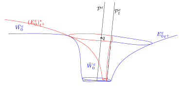
Figure 14: $\Lambda_{1}^{\varepsilon}$ attains its maximum value $t$ at $q\in\mathcal{D}^{\varepsilon}\cap\Omega$ such that $h^{\varepsilon}(q)>h_{0}^{\varepsilon}$.

Writing $z^{\varepsilon}$ for the maximum value of $\Lambda_{1}^{\varepsilon}$, it follows that

$$(E^{\varepsilon}_{0})_{t^{+}}^{*}\subset\bar{W}_{0}^{\varepsilon}\mbox{ for all }t\geq z^{\varepsilon}.$$ (41)

By letting $\varepsilon\to 0$, from (41) we get

$$E_{t^{+}}^{*}\subset\bar{W}\mbox{ for all }t\geq\limsup_{\varepsilon\to 0}z^{\varepsilon}.$$ (42)

The semicontinuity of the Alexandrov function, Lemma 13, and Claim B imply that

$$\limsup_{\varepsilon\to 0}z^{\varepsilon}\leq\Lambda(0).$$

Given $t\geq\Lambda(0)$, then $\displaystyle t\geq\limsup_{\varepsilon\to 0}z^{\varepsilon}$ by the inequality above, thus (42) says that

$$E_{t^{+}}^{*}\cap\{p\in\mathbb{R}^{3}:h(p)>\rho\}\subset\bar{W}.$$

Hence, using Claim A, we have proven that the function $\Lambda$ is non-increasing.

To finish the proof of the lemma, note that the function $\Lambda$ is either strictly decreasing or constant in some interval. In the second case, the Alexandrov function $\Lambda_{1}$ has a local interior maximum and Lemma 12 determines the existence of a plane of symmetry parallel to $\mathcal{P}$. ∎

4.3 A Schoen type theorem for ESWMT-surfaces

In this section we will establish a Schoen type theorem for ESWMT-surfaces.

Theorem 19.

Let $\Sigma\subset\mathbb{R}^{3}$ be a complete connected ESWMT-surface satisfying (1) of finite total curvature, two ends and embedded outside a compact set. Then $\Sigma$ must be rotationally symmetric. In fact, there exists $\tau>0$ such that $\Sigma$ is the surface of revolution $M_{\tau}$ determined by Sa Earp and Toubiana in [44].

Proof.

Let $E_{1}$ and $E_{2}$ be the ends of $\Sigma$. By Lemma 11 we know that $E_{1}$ and $E_{2}$ are parallel ends and $\Sigma$ grows infinitely in opposite directions. On the other hand by Theorem 18 we have that $\Sigma$ is embedded.

Let $\nu$ be the continuous extension of the Gauss map of one of the ends (observe that the Gauss map goes to $-\nu$ at the other end) and $\mathcal{P}$ a plane containing $\nu$; up to a rigid motion we can assume $\nu=(0,0,1)$ and $\mathcal{P}$ is a vertical plane. In order to apply Lemma 15 we will consider the Alexandrov functions associated to each end $E_{1}$ and $E_{2}$ (with respect to $\mathcal{P}$) denoted by $\Lambda^{1}$ and $\Lambda^{2}$ respectively. Then either both of these Alexandrov functions are strictly decreasing or at least one of the ends has a plane of symmetry parallel to $\mathcal{P}$. In the second case it is clear that the geometric comparison principle, Theorem 17, implies that $\Sigma$ has a plane of symmetry parallel to $\mathcal{P}$. For the first case we will consider the Alexandrov function associated to the entire surface $\Sigma$. This function is clearly defined over $\mathbb{R}$ since $\Sigma$ grows infinitely in opposite directions. This function is now strictly increasing on some interval $(-\infty,a]$ and strictly decreasing on some interval $[b,\infty)$, which means that the maximum value is attained on the compact set $[a,b]$; which is a global maximum, see Figure 15. This maximum value must be attained at an interior point and Lemma 12 guaranties that $\Sigma$ has a plane of symmetry parallel to $\mathcal{P}$.

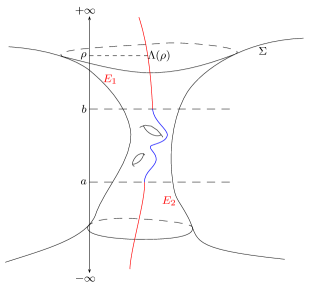
Figure 15: The associated Alexandrov function, $\Lambda$, on $\Sigma$.

Therefore, for any vertical plane, $\mathcal{P}$, $\Sigma$ is symmetric respect to some plane parallel to $\mathcal{P}$. Since the center of mass of any cross section must be contained in any plane of symmetry, then all vertical planes of symmetry intersect in a line parallel to $\nu$. Hence, $\Sigma$ is rotationally symmetric respect to this line.

By Theorem 1 there is a unique rotationally symmetric $f$-surface $M_{\tau}$ for each $\tau>0$. By the uniqueness of the ESWMT-surfaces rotationally symmetric, Theorem 4, we finally obtain that $\Sigma=M_{\tau}$. ∎

5 Applications of the Jorge-Meeks type formula

In this last section we will apply the results on Section 3 and Section 4 in order to classify ESWMT-surface of finite total curvature depending on an upper bound of the total curvature.

Theorem 20.

Let $\Sigma\subset\mathbb{R}^{3}$ be a complete ESWMT-surface satisfying (1) of finite total curvature and embedded outside a compact set. Then,

• if $\left|\int_{\Sigma}K\,dA\right|<4\pi$, $\Sigma$ is a plane;

• if $\left|\int_{\Sigma}K\,dA\right|<8\pi$, $\Sigma$ is either a plane or a special catenoid.

Proof.

Since there are no compact ESWMT-surfaces, the number of ends must be greater or equal to one; that is, $k\geq 1$. Then, if the total curvature is less than $4\pi$, by the Jorge-Meeks type formula (33), we have $g=0$ and $k=1$. Then, Theorem 9 implies that $\Sigma$ is a plane. If the total curvature is less than $8\pi$, the possibilities are $g=1$ and $k=1$ or $g=0$ and $k=2$. In the first case, $\Sigma$ must be a plane by Theorem 9; in the second case $\Sigma$ is a special catenoid by Theorem 19. ∎

References

- [1] N. Achieser. Theory of approximation. Dover publications, inc., 1992.
- [2] L. Ahlfors. Lectures on Quasiconformal Mappings. D. Van Nostrand Company, Inc, 1966.
- [3] J. Aledo, J. Espinar, and J. Gálvez. The Codazzi equation for surfaces. Advances in Mathematics, 224:2511–2530, 2010.
- [4] A. Aleksandrov. Uniqueness theorems for surfaces in the large, I. Vestnik Leningrad University: Mathematics, 11:5–17, 1956.
- [5] S. Axler, P. Bourdon, and R. Wade. Harmonic Function Theory. Springer-Verlag New York, 2001.
- [6] S. Bernstein. Sur une théorème de géometrie et ses applications aux équations dérivées partielles du type elliptique. Communications de la Société Mathématique de Kharkow, 15(1):38–45, 1915.
- [7] F. Braga and R. Sa Earp. On the structure of certain Weingarten surfaces with boundary a circle. Annales de la faculté des sciences de Toulouse, 6(2):243–255, 1997.
- [8] R. Bryant. Complex analysis and a class of Weingarten surfaces. arXiv: 1105.5589v1 [math.DG]. Preprint, 2011.
- [9] H. Chan. Nonexistence of nonpositively curved surfaces with one embedded end. Manuscripta Mathematica, 102:177–186, 2000.
- [10] H. Chan and A. Treibergs. Nonpositively curved surfaces in . Journal of Differential Geometry, 57:389–407, 2001.
- [11] S. Chern. Some new characterizations of the Euclidean sphere. Duke Mathematical Journal, 12:279–290, 1945.
- [12] S. Chern. On special W-surfaces. Proceedings of the American Mathematical Society, 6(5):783–786, 1955.
- [13] S. Chern and R. Osserman. Complete minimal surfaces in euclidean -space. Journal d’Analyse Mathématique, 19(1):15–34, 1967.
- [14] P. Connor, K. Li, and M. Weber. Complete embedded harmonic surfaces in . Experimental Mathematics, 24(2):196–224, 2015.
- [15] M. do Carmo. Differential geometry of curves and surfaces. Prentice-Hall, 1976.
- [16] J. Espinar. La ecuación de Codazzi en superficies. PhD thesis, Universidad de Granada, 2008.
- [17] R. Finn. On normal metrics, and a theorem of Cohn-Vossen. Bulletin of the American Mathematical Society, 70:772–773, 1964.
- [18] R. Finn. On a class of conformal metrics, with applications to differential geometry in the large. Commentarii Mathematici Helvetici, 40(1):1–30, 1965.
- [19] V. Gutlyanskii, V. Ryazanov, U. Srebro, and E. Yakubov. The Beltrami Equation. A Geometric Approach. Springer-Verlag New York, 2012.
- [20] J. Gálvez, A. Martínez, and F. Milan. Linear Weingarten surfaces in . Monatshefte für Mathematik, 138:133–144, 2003.
- [21] J. Gálvez, A. Martínez, and J. Teruel. Complete surfaces with ends of non positive curvature. arXiv: 1405.0851 [math.DG]. Preprint, 2016.
- [22] P. Hartman and A. Wintner. Umbilical points and W-surfaces. American Journal of Mathematics, 76(3):502–508, 1954.
- [23] D. Hoffman and W. Meeks III. The strong halfspace theorem for minimal surfaces. Inventiones Mathematicae, 101:373–377, 1990.
- [24] E. Hopf. Elementäre bemerkungen über die lösungen partieller differentialgleichungen zweiter ordnung vom elliptischen typus. Sitzungsberichte Preussische Akademie der Wissenschaften, 19:147–152, 1927.
- [25] E. Hopf. On S. Bernstein’s theorem on surfaces of nonpositive curvature. Proceedings of the American Mathematical Society, 1:80–85, 1950.
- [26] E. Hopf. A theorem on the accessibility of boundary parts of an open point set. Proceedings of the American Mathematical Society, 1:76–79, 1950.
- [27] E. Hopf. A remark on linear elliptic differential equations of second order. Proceedings of the American Mathematical Society, 3(5):791–793, 1952.
- [28] H. Hopf. Differential geometry in the large, volume 1000. Springer-Verlag Berlin Heidelberg, 1983.
- [29] A. Huber. On subharmonic functions and differential geometry in the large. Commentarii Mathematici Helvetici, 32:13–72, 1957.
- [30] L. Jorge and W. Meeks III. The topology of complete minimal surfaces of finite total Gaussian curvature. Topology, 22(2):203–221, 1983.
- [31] K. Kenmotsu. Weierstrass formula for surfaces of prescribed mean curvature. Mathematische Annalen, 245:89–99, 1979.
- [32] T. Klotz and R. Osserman. Complete surfaces in with constant mean curvature. Commentarii Mathematici Helvetici, 41:313–318, 1966-1967.
- [33] N. Korevaar, R. Kusner, and B. Solomon. The structure of complete embedded surfaces with constant mean curvature. Journal of Differential Geometry, 30:465–503, 1989.
- [34] P. Li and L.-F. Tam. Complete surfaces with total finite curvature. Journal of Differentia Geometry, 33:139–168, 1991.
- [35] W. Meeks III. The topology and geometry of embedded surfaces of constant mean curvature. Journal of Differential Geometry, 27(3):539–552, 1988.
- [36] T. Milnor. Abstract Weingarten surfaces. Journal of Differential Geometry, 15:365–380, 1980.
- [37] A. Mori. On an absolute constant in the theory of quasi-conformal mappings. Journal of the Mathematical Society of Japan, 8(2):156–166, 1956.
- [38] R. Osserman. Global properties of minimal surfaces in and . Annals of Mathematics, 80(2):340–364, 1964.
- [39] R. Osserman. A survey of minimal surfaces. Van Nostrand Reinhold Company, 1969.
- [40] J. Pérez. A new golden age of minimal surfaces. Notices of the AMS, 64(4):347–358, 2017.
- [41] P. Pucci and J. Serrin. The Maximum Principle. Birkhäuser Basel, 2007.
- [42] H. Rosenberg and R. Sa Earp. The geometry of properly embedded special surfaces in ; e.g., surfaces satisfying , where and are positive. Duke Mathematical Journal, 73(2):291–306, 1994.
- [43] R. Sa Earp and E. Toubiana. A note on special surfaces in . Matemática Contemporânea, 4:108–118, 1993.
- [44] R. Sa Earp and E. Toubiana. Sur les surfaces de Weingarten spéciales de type minimal. Boletim da Sociedade Brasileira de Matemática, 26(2):129–148, 1995.
- [45] R. Sa Earp and E. Toubiana. Classification des surfaces de type Delaunay. American Journal of Mathematics, 121(3):671–700, 1999.
- [46] R. Sa Earp and E. Toubiana. Symmetry of properly embedded special Weingarten surfaces in . Transactions of the American Mathematical Society, 351(12):4693–4711, 1999.
- [47] R. Schoen. Uniqueness, symmetry, and embeddedness of minimal surfaces. Journal of Differential Geometry, 18:791–809, 1983.
- [48] K. Shiohama. Total curvatures and minimal areas of complete open surfaces. Proceedings of the American Mathematical Society, 94(2):310–316, 1985.
- [49] S. Taliaferro. On the growth of superharmonic functions near isolated sigularity, I. Journal of Differential Equations, 158:28–47, 1999.
- [50] S. Taliaferro. Isolated singularities of nonlinear elliptic inequalities. Indiana University Mathematics Journal, 50(4):1885–1898, 2001.
- [51] S. Taliaferro. Isolated singularities of nonlinear elliptic inequalities II. Asymptotic behavior of solutions. Indiana University Mathematics Journal, 55(6):1791–1812, 2006.
- [52] B. White. Complete surfaces of finite total curvature. Journal of Differential Geometry, 26:315–326, 1987.
- [53] D. Yoon and J. Lee. Linear Weingarten helicoidal surfaces in isotropic space. Symmetry, 8(11):126, 2016.