Accelerating Experimental Design by Incorporating Experimenter Hunches

Abstract

Experimental design is a process of obtaining a product with target property via experimentation. Bayesian optimization offers a sample-efficient tool for experimental design when experiments are expensive. Often, expert experimenters have ’hunches’ about the behavior of the experimental system, offering potentials to further improve the efficiency. In this paper, we consider per-variable monotonic trend in the underlying property that results in a unimodal trend in those variables for a target value optimization. For example, sweetness of a candy is monotonic to the sugar content. However, to obtain a target sweetness, the utility of the sugar content becomes a unimodal function, which peaks at the value giving the target sweetness and falls off both ways. In this paper, we propose a novel method to solve such problems that achieves two main objectives: a) the monotonicity information is used to the fullest extent possible, whilst ensuring that b) the convergence guarantee remains intact. This is achieved by a two-stage Gaussian process modeling, where the first stage uses the monotonicity trend to model the underlying property, and the second stage uses ‘virtual’ samples, sampled from the first, to model the target value optimization function. The process is made theoretically consistent by adding appropriate adjustment factor in the posterior computation, necessitated because of using the ‘virtual’ samples. The proposed method is evaluated through both simulations and real world experimental design problems of a) new short polymer fiber with the target length, and b) designing of a new three dimensional porous scaffolding with a target porosity. In all scenarios our method demonstrates faster convergence than the basic Bayesian optimization approach not using such ‘hunches’.

I Introduction

Experimental design involves optimizing towards a target goal by iteratively modifying often large numbers of control variables and observing the result. For hundreds of years, this method has underpinned the discovery, development and improvement of almost everything around us. When experimental design entails an expensive system then Bayesian optimization [1] offers a sample-efficient method for global optimization. Bayesian optimization is a sequential, model-based optimization algorithm, which uses a probabilistic model, often a Gaussian process, as a posterior distribution over the function space. Based on the probabilistic model an utility function is constructed to seek the best location to sample next, such that the convergence towards global optima happens quickly [2]. The detail of Bayesian optimization is provided in background section II-B. It has been used in many real world design problems including alloy design [3, 4], short polymer fiber design [5], and more commonly, in machine learning hyper-parameter tuning [6, 7, 8]. However, a generic Bayesian optimization algorithm is under-equipped to harness intuitions or prior knowledge, which may be available from expert experimenters.

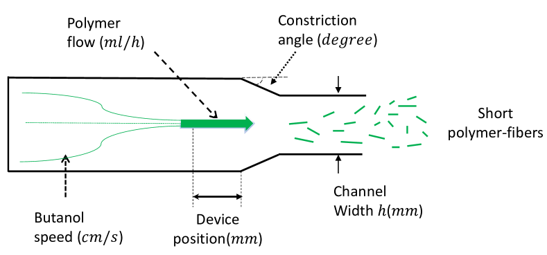
Figure 1: Short polymer fiber (SPF) synthesis using a microfluidic device. This device is parameterized by five parameters: geometric factors: channel width ($mm$), constriction angle ($degree$), and device position ($mm$); and, flow factors: coagulant (e.g. butanol) speed ($cm/s$), polymer flow ($ml/h$).

Consider the production of short polymer fibers with specific length and diameter as an experimental design problem. These fibers are used to coat natural fabrics to make them superior in many aspects e.g. more resistive to pilling, improved water repellence etc. Different types of fabrics generally require different sizes of the fibers for optimal results. The fibers are produced by injecting a polymer liquid through a high speed coagulant (e.g. butanol) flow inside a specially designed apparatus (see Figure 1). The differential speed between the polymer and the coagulant flows turns the liquid polymer into short and thin nano-scale fibers. The geometrical parameters of the apparatus and the flow speeds control the shapes and sizes of the fibers produced. In order to produce fibers with the specific length and diameter, we need to find the right values for these control parameters. Since the whole process of producing fibers is expensive, we expect to achieve the desired product by using fewer experiments. Bayesian optimization offers a perfect choice for this task. However, in this fiber production, experimenters have a prior knowledge that fiber length monotonically decreases with respect to the coagulant flow speed. Such ‘hunches’ can be directly useful in cutting down the search space if one is interested in producing either the shortest or the longest fibers. But they are not straightforwardly useful for our problem of producing fibers with a target length. In this case, such hunches do not reduce the search space, but they could still be useful in reducing the model space for model-based optimization algorithms, such as Gaussian process (GP) in Bayesian optimization. With a smaller model space to search from, it might be possible that the convergence of optimizer happens quicker.

Formally, our optimization problem based on a target $y_{T}$ can be written as,

$$\boldsymbol{x}^{*}=\text{argmin}_{\boldsymbol{x}\in\mathcal{X}}g(\boldsymbol{x})\triangleq|f(\boldsymbol{x})-y_{T}|$$ (1)

where $f(\boldsymbol{x})$ maps control variables $\boldsymbol{x}$ to the measured property. For example, in the already mentioned polymer fibre design problem, $\boldsymbol{x}$ is a vector of five parameters shown in Figure 1, $f$ is the measured fiber length and $y_{T}$ is a target length. The hunch that the experimenters posses is that fiber length is monotonically decreasing with the coagulant flow. Whilst the resultant function $g(\boldsymbol{x})$ is still a complex function over all the variables, but across the coagulant flow it is guaranteed to be unimodal. When performing Bayesian optimization, such knowledge can be useful in building a more accurate posterior Gaussian process of $g(\boldsymbol{x})$. In our experience we have found that humans are more comfortable in giving per-variable trends than multivariable ones. Also, hunches about monotonicity are more available than any more complex trends. Thus, in this work, we only consider hunches which are simple per variable monotonicity trends, which results in a target value optimization function that is unimodal in those variables.

Some of the recent work has examined various mechanisms to incorporate prior shape information into GP modeling including the enforcement on monotonicity [9, 10] and monotone-convex/concavity [11]. Wu et al. [12] has considered incorporation of exact derivative values in Bayesian optimization, but exact derivatives are hard to acquire in practice. Preliminary work [13, 14] enforces unimodality by controlling derivative sign. Unfortunately, Jauch and Pena [13] requires specification of the turning point, thus severely restricting application of their algorithms. Andersen et al. [14] needs to compute an intractable marginal from a complex joint distribution. Surprisingly, there is no details of the inference process in [14] and thus we were unable to verify or replicate their approach. Hence, we can safely conclude that none of the existing works in Bayesian optimization solves our problem where objective function is unimodal in certain dimensions, thus the problem remains open.

Our approach is based on correctly converting the monotonicity information of $f(\boldsymbol{x})$ to the unimodality information of $g(\boldsymbol{x})$ and then building a better Gaussian process model for $g(\boldsymbol{x})$. This is non-trivial since monotonicity implies a fixed sign for derivative of $f(\boldsymbol{x})$, whereas unimodality implies reversal in the sign of derivatives for $g(\boldsymbol{x})$ at the turning point. For our case we do not know the location of the turning point. In absence of turning point, a naive way can be used to derive derivative signs for $g(\boldsymbol{x})$ based on current knowledge. Specifically, based on the monotonicity direction and whether $f(\boldsymbol{x})$ is greater or smaller than the target ($y_{T}$), we can appropriately give +1 or -1 signs on some locations of $g(\boldsymbol{x})$. For example, for a minimization problem if $f(\boldsymbol{x})$ is monotonic with decreasing direction then we can put -1 at the locations where $f(\boldsymbol{x})>f_{T}$ and +1, otherwise. A more information rich GP model for $g(\boldsymbol{x})$ can be then built by combining the derived derivative signs and the available observation set $\{\boldsymbol{x},g(\boldsymbol{x})\}$ using the framework of [9]. Although this naïve idea is consistent, we show that this leads to severe under-utilization of the monotonicity information. As shown in Figure 2(b), a vast region may remain ambiguous to which sign the derivative of $g(\boldsymbol{x})$ should take.

Hence, our proposed approach is built in a two-stage process to achieve two important objectives, a) maximally use the monotonicity information, leaving no ambiguous region and b) theoretically remain consistent. We first model $f(\boldsymbol{x})$ through a Gaussian process ensuring that the mean function is monotonic in the desired variables. We then sample “virtual observations” from the posterior GP of $f(\boldsymbol{x})$ and combine them with real observations to model $g(\boldsymbol{x})$ through another Gaussian process. Since we can sample virtual observation wherever we want, we do not face the problem of having ambiguous regions again (Figure 2(d)). However, this may lead to theoretical inconsistency. The reason is, the GP model of $g(\boldsymbol{x})$ using those virtual observations not only can fix the mean function, but also may reduce the epistemic uncertainty of $g(\boldsymbol{x})$ by an equal measure. While the former is desirable, too much of the latter is undesirable, since the correct computation of epistemic uncertainty is critical for the success of Bayesian optimization [15]. To fix this, we theoretically derive an adjustment factor which corrects the overconfidence and ensures that our approach remains consistent.

We first demonstrate our methods on synthetic functions and hyperparameter tuning of neural networks. Then we solve two real world experimental design problems: a) design of short-polymer fibers with specific length, and b) design of 3d printed scaffolding with a target porosity. We use monotonicity information available from the experimenters. We demonstrate that our method outperforms the generic Bayesian optimization in these complex experimental design tasks in terms of reduced number of experimentation to reach target, saving both cost and time. The significance lies in the fact that such ’hunches’ are widely available from experimenters from almost every domain, and thus the ability of using them to accelerate experimental design process will further boost a wider adoption of Bayesian optimization in real world product and process design.

II Background

II-A Gaussian Process with Derivative Signs

Let $\boldsymbol{x}$ be a random $D$-dimensional vector in a compact set $\mathcal{X}:$ $\mathcal{X\rightarrow\mathbb{R}}$. We denote $\mathcal{D}=\{\boldsymbol{x}_{i},y_{i}\}_{i=1}^{t}$ as a set of observations, where $y_{i}=f(\boldsymbol{x}_{i})+\varepsilon_{i}$ is the noisy observation of $f(\boldsymbol{x})$ at $\boldsymbol{x}_{i}$ and $\varepsilon_{i}\sim\mathcal{N}(0,\sigma_{noise}^{2})$. A Gaussian process (GP) [16] is a random process such that every finite subset of variables has a multivariate normal distribution. A GP prior on a latent objective function $f(\boldsymbol{x})$ is fully specified by its mean function $\mu(\boldsymbol{x})=\mathbb{E}[f(\boldsymbol{x})]$ and the covariance function $k(\boldsymbol{x},\boldsymbol{x}^{{}^{\prime}})=\mathbb{E}[(f(\boldsymbol{x})-\mu(\boldsymbol{x}))(f(\boldsymbol{x}^{{}^{\prime}})-\mu(\boldsymbol{x}^{{}^{\prime}}))]$. A zero-mean GP prior is formulated as

$$f(\boldsymbol{x})\sim\mathcal{GP}(\boldsymbol{0},k(\boldsymbol{x},\boldsymbol{x}^{{}^{\prime}}))$$ (2)

The kernel function $k$ encodes the prior belief regarding the smoothness of the objective function. A popular kernel is the square exponential (SE) function $k(\boldsymbol{x}_{i},\boldsymbol{x}_{j})=\epsilon\exp(-\frac{1}{2l^{2}}||\boldsymbol{x}_{i}-\boldsymbol{x}_{j}||^{2})$, where $\epsilon$ is the output variance and $l$ is the length scale. The predictive distribution of $y^{+}$ for a test point $\boldsymbol{x}^{+}$ in GP can be computed by

$$y^{+}\mid\boldsymbol{y}_{1:t}\sim\mathcal{N}(\mathbf{k}^{T}\mathbf{K}^{-1}\boldsymbol{y}_{1:t},k(\boldsymbol{x}_{t+1},\boldsymbol{x}_{t+1})-\mathbf{k}^{T}\mathbf{K}^{-1}\mathbf{k})$$ (3)

where $\mathcal{N}$ denotes a Gaussian distribution, $\mathbf{k}=[k(\boldsymbol{x}^{+},\boldsymbol{x}_{1})\,\cdots\,k(\boldsymbol{x}^{+},\boldsymbol{x}_{t})]^{T}$ and $\mathbf{K}=[k(x_{i},x_{j})]_{i,j\in\{1,\cdots,t\}}+\sigma_{noise}^{2}\mathbf{I}$.

Since the GP is a linear operator, the derivative of Gaussian process is still a Gaussian process [9]. Therefore, incorporating derivative values into GP for prediction is straightforward since the joint distribution of derivative value and function value is still a Gaussian distribution. In our work it is hard to acquire derivative values and we only have derivative signs derived from the prior monotonicity knowledge. The derivative sign ’+1’ denotes that the gradient of latent function at the location is positive and ’-1’ denotes that the gradient is negative at this location. We follow the work in [9] to compute the posterior GP given function observations and derivative signs.

Let $\mathcal{M}=\{\boldsymbol{x}_{s_{i}},s_{i}\}_{i=1}^{m}$ denote $m$ derivative sign observations, where $s_{i}$ is the derivative sign at location $\boldsymbol{x}_{s_{i}}$. We specify the derivative sign as the partial one with respect to the $d$th variable. It is also easy to extend to any number of variables. For convenience, we denote $X=\{\boldsymbol{x}_{i}\}_{i=1}^{t}$, $X_{s}=\{\boldsymbol{x}_{s_{i}}\}_{i=1}^{m}$ and $\boldsymbol{s}=\{s_{i}\}_{i=1}^{m}$. The latent function value and the partial derivative value for the $d$th variable are denoted as $\boldsymbol{f}$ and $\boldsymbol{f}^{{}^{\prime}}$ respectively.

In Gaussian process regression, the goal is to compute the posterior predictive distribution of a test point. Similarly, given observations and derivative signs we can express the predictive distribution of a test point $\boldsymbol{x}^{+}$ by integrating out the latent $\boldsymbol{f}$ and $\boldsymbol{f}^{{}^{\prime}}$

$$p(y^{+}\mid\boldsymbol{x}^{+},X,\boldsymbol{y},X_{s},\boldsymbol{s})=$$

$$\int p(y^{+}\mid\boldsymbol{x}^{+},X,\boldsymbol{y},\boldsymbol{f,}X_{s},\boldsymbol{s},\boldsymbol{f}^{{}^{\prime}})p(\boldsymbol{f},\boldsymbol{f}^{{}^{\prime}}\mid X,\boldsymbol{y},X_{s},\boldsymbol{s})d\boldsymbol{f}d\boldsymbol{f}^{{}^{\prime}}$$ (4)

The first term $p(y+\mid\boldsymbol{x}^{+},X,\boldsymbol{y},\boldsymbol{f},X_{s},\boldsymbol{s},\boldsymbol{f}^{{}^{\prime}})$ at the right side above is a Gaussian distribution (see [9]) and the second term is the joint posterior distribution of $\boldsymbol{f}$ and $\boldsymbol{f}^{{}^{\prime}}$. The second term can be computed by

$$p(\boldsymbol{f},\boldsymbol{f}^{\boldsymbol{{}^{\prime}}}\mid X,\boldsymbol{y},X_{s},\boldsymbol{s})=\frac{1}{Z}p(\boldsymbol{f},\boldsymbol{f}^{{}^{\prime}}\mid X,X_{s})p(\boldsymbol{y}\mid\boldsymbol{f})p(\boldsymbol{s}\mid\boldsymbol{f^{{}^{\prime}}})$$ (5)

where $Z$ is a normalization term and $p(\boldsymbol{f},\boldsymbol{f}^{{}^{\prime}}|X,X_{s})$ is the joint prior between $\boldsymbol{f}$ and $\boldsymbol{f}^{{}^{\prime}}$ which can be computed by

$$p(\boldsymbol{f},\boldsymbol{f}^{{}^{\prime}}\mid X,X_{s})=\mathcal{N}\left(\boldsymbol{f}_{joint}\mid\boldsymbol{0},K_{joint}\right)$$ (6)

where $\boldsymbol{f}_{joint}=\left[\begin{array}[]{c}\boldsymbol{f}\\ \boldsymbol{f}^{{}^{\prime}}\end{array}\right]$, $K_{joint}=\left[\begin{array}[]{cc}K_{XX}&K_{XS}\\ K_{SX}&K_{SS}\end{array}\right],$$K_{XX}$ and $K_{SS}$ are the self-covariance matrix of $X$ and $X_{s}$, respectively and $K_{XS}$ is the covariance matrix between $X$ and $X_{s}$.

In Eq.(5), $p(\boldsymbol{s}|\boldsymbol{f^{{}^{\prime}}})$ is the likelihood of derivative sign conditioning on derivative value. Therefore, one has to build the link between derivative sign $\boldsymbol{s}$ and derivative value $\boldsymbol{f}^{{}^{\prime}}$ in order to compute Eq.(5) . Riihimaki and Vehtari [9] suggest using a probit function to represent the likelihood of derivative signs over latent derivative values as,

$$p(\boldsymbol{s}\mid\boldsymbol{f})=\prod_{i=1}^{m}\Phi\left(\frac{s_{i}\partial f^{(i)}}{\partial x_{d}^{(i)}}\frac{1}{\nu}\right)$$ (7)

where $\Phi(z)=\int_{-\infty}^{z}\mathcal{N}(x\mid 0,1)dx$ and the steepness $\nu$ indicates the consistency between the derivative values and derivative signs. If we are confident about the derivative signs, we set $\nu$ as a small value, otherwise large. Since the likelihood in Eq.(7) is not Gaussian, Eq.(5) is intractable analytically. Similar with the GP classification [16], Riihimaki and Vehtari [9] used expectation propagation (EP) [17] to approximate Eq.(5). Briefly, we can use EP to approximate Eq.(5) as

$$q(\boldsymbol{f},\boldsymbol{f}^{{}^{\prime}}\mid X,\boldsymbol{y},X_{s},\boldsymbol{s})$$

$$=\frac{1}{Z}p(\boldsymbol{f},\boldsymbol{f}^{{}^{\prime}}\mid X,X_{s})p(\boldsymbol{y}\mid\boldsymbol{f})\prod_{i=1}^{N}t_{i}(f_{i}\mid Z_{i},\mu_{i},\sigma_{i})$$

where $t_{i}(f_{i}\mid\tilde{Z}_{i},\tilde{\mu}_{i},\tilde{\sigma}_{i}^{2})\simeq\tilde{Z}_{i}\mathcal{N}(f_{i}\mid\tilde{\mu}_{i},\tilde{\sigma}_{i}^{2})$, which defines a un-normalized Gaussian function with site parameter $\tilde{Z}_{i}$, $\tilde{\mu_{i}}$ and $\tilde{\sigma}_{i}^{2}$. Therefore Eq.(5) would be a product of multiple Gaussian distributions after approximation. The detail inference can be found in [9]. Then the predictive mean and variance of GP with derivative signs in Eq.(4) can be derived and they have the similar form with those in the standard GP.

If we set derivative signs with respect to one variable to be always negative or positive, the resulted Gaussian process will be modeled towards the desired monotonic shape on this variable. We denote it as monotonic GP. Usually the higher the number of sign observations (that is a larger $m$), stronger is the monotonicity imposition. However, due to the complexity $O((t+m)^{3})$ in GP with derivative signs, it is not practical working with many derivative signs. In our experiments, we place about five derivative signs per monotonic dimension equally spaced within the bound of the variable.

II-B Bayesian Optimization

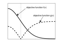
(a)

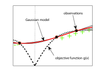
(b)

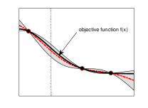
(c)

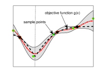
(d)

Figure 2: Illustration of the problem and solutions. (a) Objective function $f(\boldsymbol{x})$ is monotonically decreasing and $g(\boldsymbol{x})=|f(\boldsymbol{x})-y_{T}|$. The vertical dotted line is the location of the target $y_{T}$. (b) BO-DS: Posterior GP of $g(\boldsymbol{x})$. The red dotted line represents the mean function and the shadow represents predicted variance. The derivative signs of $g(\boldsymbol{x})$ are derived based on the monotonicity of $f(\boldsymbol{x})$. Information about derivative sign is lacking in regions as discussed in text; (c) BO-MG: Posterior GP of $f(\boldsymbol{x})$, incorporating knowledge that $f(\boldsymbol{x})$ is monotonically decreasing. (d) BO-MG: Posterior GP of $g(\boldsymbol{x})$ combining points sampled from GP in (c) and actual observations.

Bayesian optimization (BO) is an efficient tool to globally optimize an expensive black-box function. It is a greedy search procedure guided by a surrogate function that is analytical and cheap to evaluate. Typically, we use Gaussian process to model the latent function in BO. The posterior mean and variance at each point can be analytically derived based on Eq.(3). Then the surrogate function (or called acquisition function) is constructed using both the predictive mean and variance. The next sample location $\boldsymbol{x}_{t+1}$ is found by maximizing the acquisition function and then $y_{t+1}$ is obtained after performing a new experiment with $\boldsymbol{x}_{t+1}$. The new observation $\{\boldsymbol{x}_{t+1},y_{t+1}\}$ is augmented to update the GP. These steps are repeated till a satisfactory outcome is reached or the iteration budget is exhausted. We present a generic BO in Alg. 1.

The acquisition function is designed to trade-off between exploitation of high predictive mean and exploration of high epistemic uncertainty. Choices of acquisition functions include Expected Improvement (EI) [2], GP-UCB [2] and entropy search [18]. In this paper we use GP-LCB for a minimization problem, which minimizes the acquisition function

$$a_{t}(\boldsymbol{x})=\mu_{t-1}(\boldsymbol{x})-\sqrt{\alpha_{t}}\sigma_{t-1}(\boldsymbol{x})$$ (8)

where $\alpha_{t}$ is a positive trade-off parameter, $\mu_{t-1}(\boldsymbol{x})$ is the predicted mean and $\sigma_{t-1}(\boldsymbol{x})$ is the predicted variance.

Simple regret at $t$th iteration is defined as $r_{t}=f(\boldsymbol{x}_{t})-f(\boldsymbol{x}^{*})$ for minimization problem where $\boldsymbol{x}^{*}$ is the global optima of $f(\boldsymbol{x})$. Srinivas et al. [2] theoretically analyzed the regret bound of BO using the GP-LCB acquisition function and showed that a) Bayesian optimization with GP-LCB is a no-regret algorithm and b) the cumulative regret ($R_{T}=\sum_{t=1}^{T}r_{t}$) grows only sub-linearly, i.e. the convergence rate is the fastest among all global optimizers known so far.

Algorithm 1 The standard Bayesian Optimization

1:  for $t=1,2\cdots$ do

2:     Optimize for the next point $\boldsymbol{x}_{t+1}$$\leftarrow$$\text{argmax}_{\boldsymbol{x}_{t+1\in\boldsymbol{X}}}a(\boldsymbol{x}\mid\mathcal{D}_{1:t})$

3:     Evaluate the value $y_{t+1}$

4:     Augment the data $\mathcal{D}_{1:t+1}=\{\mathcal{D}_{1:t},\{\boldsymbol{x}_{t+1},y_{t+1}\}\}$

5:     Update the kernel matrix $\mathbf{K}$

6:  end for

III Bayesian Optimization with Monotonicity Information

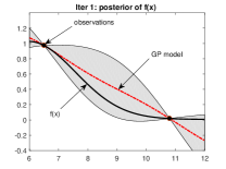
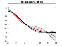
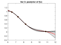
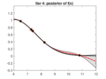
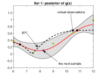
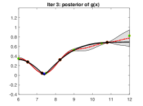
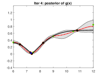
Figure 3: The behavior of BO-MG on a 1-d example with $y_{T}=0.7$. The topmost plots shows the posterior of $f(\boldsymbol{x})$ by using monotonic GP. The plots in the bottom row depict the posterior of $g(\boldsymbol{x})$ after introducing the virtual observations sampled from the posterior GP of $f(\boldsymbol{x})$ (denoted by green dots). The shade denotes the region covered by three times of the predictive variance.

Our objective is to reach a target value $y_{T}$ given the monotonicity of $f(\boldsymbol{x})$. A natural choice is to minimize the difference between the target and function values - Eq.(1). We now discuss how to incorporate the monotonicity of $f(\boldsymbol{x})$ into BO to improve efficiency.

Algorithm 2 Bayesian optimization with derivative signs

0:  observations $\mathcal{D}_{1:t}=\{\boldsymbol{x_{i}},y_{i}\}_{i=1}^{t}$, the target value $y_{T}$, the monotonicity with respect to the $d$th variable.

1:  for $t=1,2,\cdots$ do

2:     derive derivative sign observations $\mathcal{M}=\{\boldsymbol{x}_{s_{i}},s_{i}\}_{i=1}^{M}$ on $g(\boldsymbol{x})$ (Lemma 1).

3:     obtain observations $\mathcal{G}=\{\boldsymbol{x}_{i},|y_{i}-y_{T}|\}_{i=1}^{t}$;

4:     build GP on $g(\boldsymbol{x})$ with $\mathcal{G}$ and $\mathcal{M}$ (Sec II-A);

5:     optimize for the next point $\boldsymbol{x}_{t+1}$$\leftarrow$$\text{argmax}_{\boldsymbol{x}_{t+1\in\mathcal{X}}}a(\boldsymbol{x}\mid\mathcal{G},\mathcal{M})$

6:     evaluate the function $y_{t+1}=f(\boldsymbol{x}_{t+1})+\varepsilon$;

7:     augment the data $\mathcal{D}_{1:t+1}=\{\mathcal{D}_{1:t},\{\boldsymbol{x}_{t+1},y_{t+1}\}\}$;

8:  end for

III-A Bayesian Optimization with Derivative Signs (BO-DS)

A naïve method to utilize the monotonicity information is to derive the property of $g(\boldsymbol{x})$ based on the given monotonicity of $f(\boldsymbol{x})$ and locations of observations. We derive derivative signs of $g(\boldsymbol{x})$ through the Lemma as follows:

Lemma 1.

Let $f(\boldsymbol{x})$ be a monotonically decreasing function with respect to the $d$th variable. Given the search bound $[L_{d},U_{d}]$ of the $d$’th variable and an observation $\{\boldsymbol{x}_{i},y_{i}\}$($\boldsymbol{x}_{i}=[x_{i1},\cdots,x_{id},\cdots,x_{iD}]$), if $y_{i}>y_{T}$, then $s<0$ at $\boldsymbol{x}_{s}=[x_{i1},\cdots,l_{s},\cdots,x_{iD}]$ for $\forall l_{s}\in[L_{d},x_{nd}]$ and if $y_{i}<y_{T}$, then $s>0$ at $\boldsymbol{x}_{s}=[x_{i1},\cdots,l_{s},\cdots,x_{iD}]$ for $\forall l_{s}\in[x_{id},U_{d}]$.

Proof: Since $f(\boldsymbol{x})$ is monotonically decreasing with respect to the $d$th variable, then $f(\boldsymbol{x}_{s})>y_{i}$ for $l_{s}<x_{nd}$. Further we can get $|f(\boldsymbol{x}_{s})-y_{T}|>|y_{i}-y_{T}|$ if $y_{i}>y_{T}$. It means that $g(\boldsymbol{x}_{s})>g_{i}$ and we can obtain the derivative sign $s<0$ at $\boldsymbol{x}_{s}$. We can similarly prove the latter statement in Lemma 1. This lemma is easy to extend to multiple dimensional case.

Once a set of derivative signs $\mathcal{M}=\{\boldsymbol{x}_{s_{i}},s_{i}\}_{i=1}^{m}$ on $g(\boldsymbol{x})$ is acquired in this way, they are combined with the actual observations $\mathcal{G}=\{\boldsymbol{x}_{i},|y_{i}-y_{T}|\}_{i=1}^{t}$. Then a GP model can be constructed using the method of GP with derivative signs in section II-A and BO is performed on $g(\boldsymbol{x})$ to acquire the next recommendation. We term this algorithm BO with Derivative Signs (BO-DS), which is presented in Alg. 2 .

A crucial drawback of this algorithm is that we do not know any derivative information around the optimum, only away from it (See Figure 2(b)). Thus we have only partially exploited the monotonicity information of $f(\boldsymbol{x})$ in this approach.

III-B Bayesian Optimization with Monotonic GP (BO-MG)

To overcome the drawback of BO-DS, we develop a two-stage algorithm to eliminate the ambiguity of derivative signs in search bound. We first model the mean function of posterior GP of $f(\boldsymbol{x})$ as a monotonic function, then sample points from this GP and combine them with existing actual observations to build a new GP model for $g(\boldsymbol{x})$. Thus we make full use of the monotonicity of $f(\boldsymbol{x})$ and transfer this critical knowledge to $g(\boldsymbol{x})$ through a set of sampled points.

In detail, we model $f(\boldsymbol{x})$ using monotonic GP by placing the consistent derivative signs $\{\boldsymbol{x}_{s},s\}$ across the search space. We then sample $N$ points $X_{v}=\{\boldsymbol{x}_{j}^{v}\}_{j=1}^{N}$ from this monotonic GP. We denote the sampled set $\mathcal{V}=\{\boldsymbol{x}_{j}^{v},\mu_{f}(\boldsymbol{x}_{j}^{v}),\sigma_{f}^{2}(\boldsymbol{x}_{j}^{v})\}_{j=1}^{N}$ with the mean and variance. We note that it is important to retain $\sigma_{f}^{2}(\boldsymbol{x}_{j}^{v})$ to maintain proper epistemic uncertainty. Combining sampled points and existing observations $\mathcal{G}=\{\boldsymbol{x}_{i},|y_{i}-y_{T}|\}_{i=1}^{t}$, we construct a new GP on $g(\boldsymbol{x})$ and then perform Bayesian optimization. The mean and variance for a new point $\boldsymbol{x}_{t+1}$ in this GP are

$$\mu_{g}(\boldsymbol{x}_{t+1})=\mathbf{k}^{T}K^{-1}[\boldsymbol{\mu}_{g}(X_{v});|\boldsymbol{y}-y_{T}|]$$ (9)

$$\sigma_{g}^{2}(\boldsymbol{x}_{t+1})=k(\boldsymbol{x}_{t+1},\boldsymbol{x}_{t+1})-\mathbf{k}^{T}K^{-1}\mathbf{k}$$ (10)

where $\boldsymbol{\mu}_{g}(X_{v})=|\boldsymbol{\mu}_{f}(X_{v})-y_{T}|$, $\mathbf{k}=[k(\boldsymbol{x}_{t+1},\boldsymbol{x}_{1}^{v})\,\cdots\,k(\boldsymbol{x}_{t+1},\boldsymbol{x}_{N}^{v})\,k(\boldsymbol{x}_{t+1},\boldsymbol{x}_{1})\,\cdots\,k(\boldsymbol{x}_{t+1},\boldsymbol{x}_{t})]$ and

$$K=\left[\begin{array}[]{cc}K_{VV}&K_{VX}\\ K_{XV}&K_{XX}\end{array}\right]+\left[\begin{array}[]{cc}\boldsymbol{\sigma}_{f}^{2}(X_{v})&\boldsymbol{0}\\ \boldsymbol{0}&{}_{\sigma_{noise}^{2}}\end{array}\right]\text{I}$$ (11)

and $K_{VV}$ is the self-covariance matrix of $X_{v}$ and $K_{XV}$ is the covariance matrix between $X$ and $X_{v}$. The overall algorithm is presented in Alg 3. The comparison between BO-MG and BO-DS algorithms is illustrated in Figure 2. To further show how BO-MG behaves we demonstrate this algorithm in 1-d example in Figure 3. The BO-MG can model the true mean function of $g(\boldsymbol{x})$ very well and converge the optimum quickly.

A crucial step in BO-MG is to sample points from monotonic GP and merge them with actual observations to build a new GP model, which we denote as the combined GP. Adding sample points (virtual observations) to the combined GP may reduce predictive variance. An undesirable side effect is that it may result in the overconfidence in exploitation due to the shrinkage of the epistemic uncertainty resulted from more observations. To guarantee the algorithm’s convergence, we need to control for this overconfidence. If not corrected, it will avoid exploration at the cost of exploitation for the combined GP. For the acquisition function GP-LCB, a way to avoid overconfidence is to adjust the trade-off parameter so that the exploration can be increased. We analyze the setting of trade-off parameter in the next section.

Algorithm 3 Bayesian optimization with monotonic GP

0:  observations $\mathcal{D}_{1:t}=\{\boldsymbol{x_{i}},y_{i}\}_{i=1}^{t}$, the target value $y_{T}$, the monotonicity with respect to the $d$th variable

1:  for $t=1,2,\cdots$ do

2:     build monotonic GP on $f(\boldsymbol{x})$ using the consistent derivative signs (Sec II-A);

3:     sample virtual observations $\mathcal{V}$ from the monotonic GP above (Sec III-B);

4:     obtain observations $\mathcal{G}=\{\boldsymbol{x}_{i},|y_{i}-y_{T}|\}_{i=1}^{t}$;

5:     build GP on $g(\boldsymbol{x})$ using $\mathcal{V}$ and $\mathcal{G}$ (Sec III-B);

6:     sample $\boldsymbol{x}_{t+1}$$\leftarrow$$\text{argmax}_{\boldsymbol{x}_{t+1\in\mathcal{X}}}a(\boldsymbol{x}\mid\mathcal{G},\mathcal{V})$;

7:     evaluate the function $y_{t+1}=f(\boldsymbol{x}_{t+1})+\varepsilon$;

8:     augment the data $\mathcal{D}_{1:t+1}=\{\mathcal{D}_{1:t},\{\boldsymbol{x}_{t+1},y_{t+1}\}\}$;

9:  end for

III-C Theoretical Analysis for BO-MG

We denote $g$ as a sample from the combined GP model. With $N_{1}$ sampled points, the GP-LCB decision rule for the next point is given as

$$\boldsymbol{x}_{t}^{N_{1}}=\underset{{}_{\boldsymbol{x}\in\mathcal{X}}}{\text{argmin}\ }\mu_{t}^{N_{1}}(\boldsymbol{x})-\sqrt{\alpha_{t}}\sigma_{t-1}^{N_{1}}(\boldsymbol{x})$$ (12)

where $\mu_{t-1}^{N_{1}}(\boldsymbol{x})$ and $\sigma_{t-1}^{N_{1}}(\boldsymbol{x})$ are the predictive mean and variance in this GP. With $N_{2}$ ($N_{2}>N_{1}$ and $\boldsymbol{x}_{1:N_{1}}\subset\boldsymbol{x}_{1:N_{2}}$) sampled points, the decision rule is

$$\boldsymbol{x}_{t}^{N_{2}}=\underset{{}_{\boldsymbol{x}\in\mathcal{X}}}{\text{argmin}\ }\mu_{t-1}^{N_{2}}(\boldsymbol{x})-\sqrt{\beta_{t}}\sigma_{t-1}^{N_{2}}(\boldsymbol{x})$$ (13)

where $\mu_{t-1}^{N_{2}}(\boldsymbol{x})$ and $\sigma_{t-1}^{N_{2}}(\boldsymbol{x})$ are corresponding predictive mean and variance.

Suppose these two GPs use the same hyperparameters, then $\mu_{t-1}^{N_{1}}(\boldsymbol{x})$ is approximately equal to $\mu_{t-1}^{N_{2}}(\boldsymbol{x})$ and $\sigma_{t-1}^{N_{2}}(\boldsymbol{x})$ is less than $\sigma_{t-1}^{N_{1}}(\boldsymbol{x})$ due to the introduction of sampled points for $\forall t$ and $\forall\boldsymbol{x}\in\mathcal{X}$. To overcome the overconfidence in exploitation of the combined GP, we must choose a proper $\beta_{t}$ to increase its confidence intervals so that $\sqrt{\beta_{t}}\sigma_{t-1}^{N_{2}}(\boldsymbol{x})$ can contain $\sqrt{\alpha_{t}}\sigma_{t-1}^{N_{1}}(\boldsymbol{x})$ for $\forall t$ and $\forall\boldsymbol{x}\in\mathcal{X}$, i.e.

$$\sqrt{\beta_{t}}\sigma_{t-1}^{N_{2}}(\boldsymbol{x})\geq\sqrt{\alpha_{t}}\sigma_{t-1}^{N_{1}}(\boldsymbol{x})$$ (14)

We use the choice of $\alpha_{t}$ derived by [2]. The core task becomes to bound the ratio

$$r_{t-1}(\boldsymbol{x})=\sigma_{t-1}^{N_{1}}(\boldsymbol{x})/\sigma_{t-1}^{N_{2}}(\boldsymbol{x})$$ (15)

As in [15], this ratio can be computed by the proposition as follows:

Proposition 2.

The ratio of the standard deviation of the posterior over $g(\boldsymbol{x})$, conditioned on observations $y_{1:t-1}$ and $N_{1}$ sampled points to that when $g(\boldsymbol{x})$ is conditioned on observations $y_{1:t-1}$ and $N_{2}$ sampled points is

$$\frac{\sigma_{t-1}^{N_{1}}(\boldsymbol{x})}{\sigma_{t-1}^{N_{2}}(\boldsymbol{x})}=\exp\left(I(g(\boldsymbol{x});y_{(N_{1}+1):N_{2}}\mid y_{1:t-1}\cup y_{1:N_{1}}\right)$$ (16)

We prove it by expanding the mutual information as follows:

$$I(g(\boldsymbol{x});y_{(N_{1}+1):N_{2}}\mid y_{1:t-1}\cup y_{1:N_{1}})$$

$$=H(g(\boldsymbol{x})\mid y_{1:t-1}\cup y_{1:N_{1}})-H(g(\boldsymbol{x})\mid y_{1:t-1}\cup y_{1:N_{2}})$$

$$=\frac{1}{2}\log\left(2\pi e\sigma_{t-1}^{N_{1}}(\boldsymbol{x})\right)-\frac{1}{2}\log\left(2\pi e\sigma_{t-1}^{N_{2}}(\boldsymbol{x})\right)$$

$$=\log\left(\sigma_{t-1}^{N_{1}}(\boldsymbol{x})/\sigma_{t-1}^{N_{2}}(\boldsymbol{x})\right)$$

It shows that there exists a constant $C$ such that $I(g(\boldsymbol{x});y_{(N_{1}+1):N_{2}}\mid y_{1:t-1}\cup y_{1:N_{1}})\leq C$ for $\forall t$ and $\forall\boldsymbol{x}\in\mathcal{X}$. Therefore we can successfully bound $r_{t-1}(\boldsymbol{x})\leq\exp(C)$.

By the monotonicity and submodularity properties of mutual information [15, 19], we get:

$$I(g(\boldsymbol{x});y_{(N_{1}+1):N_{2}}\mid y_{1:t-1}\cup y_{1:N_{1}})$$

$$\leq I(g;y_{(N_{1}+1):N_{2}}\mid y_{1:t-1}\cup y_{1:N_{1}})$$ (17)

$$\leq\max_{\mathcal{A}\subseteq\mathcal{X},|\mathcal{A}|\leq N_{2}-N_{1}}I(g;y_{\mathcal{A}}\mid y_{1:t-1}\cup y_{1:N_{1}})$$ (18)

$$\leq\max_{\mathcal{A}\subseteq\mathcal{X},|\mathcal{A}|\leq N_{2}-N_{1}}I(g;y_{\mathcal{A}})=\gamma_{N_{2}-N_{1}}$$ (19)

Generally $\gamma_{N_{2}-N_{1}}$ is difficult to calculate since it generally requires to compute the information gain for all combinations of $(N_{2}-N_{1})$ points. Fortunately, Andreas and Carlos [19] demonstrated an easy method to obtain upper bound on $\gamma_{N_{2}-N_{1}}$. Specifically, they show

$$\gamma_{N_{2}-N_{1}}\leq\frac{e}{e-1}I(g;y_{N_{2}-N_{1}})$$ (20)

where $I(g;y_{N_{2}-N_{1}})$ the information gain by observing the set of observations $y_{(N_{1}+1):N_{2}}$ of the actions $\{\boldsymbol{x}_{N_{1}+1},\cdots,\boldsymbol{x}_{N_{2}}\}$ selected using uncertainty sampling [15]. It implies that we can use uncertainty sampling to select $N_{2}-N_{1}$ sampled points in BO-MG such that we can obtain $C$. With $C=\gamma_{N_{2}-N_{1}}$, we can get the regret bound as follows:

Theorem 3.

Let $\delta\in(0,1)$ and run BO-MG with GP-LCB decision rule with $\beta_{t}=\exp(2C)\alpha_{t}$, we get a cumulative regret bound $R_{T}$ with a high probability

$$\text{Pr}\{R_{T}\leq\sqrt{C_{1}T\exp(2\gamma_{N_{2}-N_{1}})\alpha_{t}\gamma_{T}}+2,\forall T\geq 1\}=1-\delta$$ (21)

where $C_{1}=8/\log(1+\sigma_{noise}^{2})$, $\gamma_{T}$ is the maximum information gain between the function values $f_{1:T}$ and the noisy observations $y_{1:T}$ , $\gamma_{N_{2}-N_{1}}$ is defined in Eq.(19), and $\alpha_{t}=2\log(2t^{2}\pi^{2}/(3\delta))+2d\log\left(dt^{2}bl\sqrt{\log(4da/\delta)}\right)$.

The proof is similar to that in [2].

Discussion

We have explicitly discussed that the convergence rate of BO-MG can be guaranteed if $\beta_{t}=\exp(2C)\alpha_{t}$ and $C=\gamma_{N_{2}-N_{1}}$. In practice, $N_{1}$ can be a very small one and then the maximum information gain $\gamma_{N_{2}-N_{1}}$ grows with the size of $N_{2}$ and $C$ would be very large and thus the algorithm tends to over-explore if we use the computed $C$ for $\beta_{t}$. Fortunately we can also set $\beta_{t}=\left(\max\left(r_{t-1}(\boldsymbol{x})\right)\right)^{2}\alpha_{t}$ in order to guarantee $\beta_{t}\geq r_{t-1}^{2}(\boldsymbol{x})\alpha_{t}$ (Eq. 14) for $\forall t$ and $\forall\boldsymbol{x}\in\mathcal{X}$. Actually we can obtain the maximal value of $r_{t-1}(\boldsymbol{x})$ by maximizing Eq.(15) for $\forall\boldsymbol{x}\in\mathcal{X}$ at iteration $t$. In this way we can guarantee the convergence of BO-MG. For good practical performance, a more aggressive method is to reduce $\beta_{t}$ by a correction factor $\eta$ [2]

$$\beta_{t}=\left(\max\left(r_{t-1}(\boldsymbol{x})\right)\right)^{2}\eta\alpha_{t}$$ (22)

Eq.(15) indicates that the value $\max\left(r_{t-1}(\boldsymbol{x})\right)$ is increasing with $N_{2}$ (assume $N_{1}$ is fixed) and therefore we can adjust $\eta$ for different $N_{2}$ for better practical performance.

IV Experiments

We compare our proposed method with the following algorithms:

• Bayesian optimization with monotonic GP (BO-MG) which incorporates the sampled points from the monotonic GP into Bayesian optimization (Alg. 3);

• Bayesian optimization with derivative signs (BO-DS) which directly incorporates the derivative signs derived from prior monotonicity into BO (Alg. 2);

• standard Bayesian optimization (standard BO) which does not include any prior knowledge (Alg. 1).

For all three algorithms, we automatically estimate the hyperparameters of the SE kernel in GP including the length scale $l$ and the output variance $\epsilon$ and the noise variance $\sigma_{noise}^{2}$ at each iteration. Both BO-DS and BO-MG requires the GP with derivative signs. We empirically set $\nu=0.01$ and used the GPstuff toolbox [20] to implement the GP with derivative signs. The acquisition function we used for all algorithms is the GP-LCB. For standard BO and BO-DS, the trade-off parameter $\alpha_{t}$ in Eq.(8) can be set by following [2] but is scaled down with a small factor as [2] and [15] did (we use 0.1 in our experiments). For BO-MG, we used the trade-off parameter $\beta_{t}$ in Eq.(22). To compute $\max\left(r_{t-1}(\boldsymbol{x})\right)$ we sampled $N_{1}=5$, $N_{2}=10$ for 2D functions, $N_{1}=5$, $N_{2}=20$ for 5D functions and $N_{1}=5$, $N_{2}=40$ for 7D functions using Latin hypercube sampling and ensured sampled points $\boldsymbol{x}_{1:N_{1}}\subset\boldsymbol{x}_{1:N_{2}}$. BO-MG provides competitive performance with $\eta=0.1$ for 1D~5D functions and $\eta=0.01$ for 7D functions in our experiments. We run experiments for 20 trials with random initial points and report the average mean and the standard error. The code is available in https://bit.ly/2sDFQ35.

We first compared algorithms on the optimization of benchmark functions and hyperparameter tuning in neural network. We then solved two real-world applications - the optimization of short fibers with targeted length and porous architecture (scaffold) design for biomaterials with target porosity using 3D printing.

IV-A Optimization of benchmark functions

We optimize the following benchmark functions:

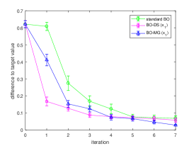
(a) 2D function $f_{1}$.

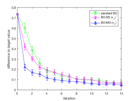
(b) 5D function $f_{2}$.

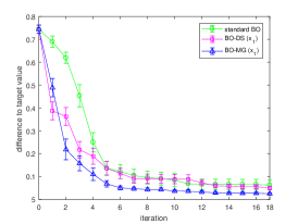
(c) 7D function $f_{3}$.

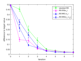
(d) 2D function $f_{4}$.

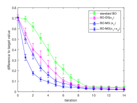
(e) 5D function $f_{5}$.

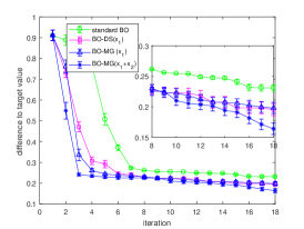
(f) 7D function $f_{6}$.

Figure 4: The results of optimizing benchmark functions. The graph shows the comparison of difference to the target value between different algorithms. The vertical axis represents the difference to the target value.

(a) 2D function: $f_{1}(\boldsymbol{x})=\frac{1}{20}(x_{1}-5){}^{2}+\frac{1}{20}(x_{2}-4){}^{2}$, $f_{T}=1.5$, $\boldsymbol{x}\in[0,5]$;

(b) 5D function: $f_{2}(\boldsymbol{x})=\frac{1}{30}(x_{1}-3){}^{2}+\frac{1}{30}(x_{2}-2){}^{2}+\mathcal{GN}(x_{3:5}|\boldsymbol{0},\boldsymbol{1})$, $f_{T}=1.5$, $\boldsymbol{x}\in[-2,3]$, where $\mathcal{GN}(x_{3:5}|0,1)$ is a un-normalized Gaussian PDF for $x_{3}\sim x_{5}$;

(c) 7D function: $f_{3}(\boldsymbol{x})=\frac{1}{30}(x_{1}-3){}^{2}+\frac{1}{30}(x_{2}-2){}^{2}+\mathcal{GN}(x_{3\text{:7}}|\boldsymbol{0},\boldsymbol{1})$, $f_{T}=1.3$, $\boldsymbol{x}\in[-3,3]$, where $\mathcal{GN}(x_{3:7}|0,1)$ is a un-normalized Gaussian PDF for $x_{3}\sim x_{7}$;

(d) 2D function: $f_{4}(\boldsymbol{x})=\frac{1}{20}(x_{1}-5)x_{2}$, $f_{T}=0.8$, $\boldsymbol{x}\in[0,5]$;

(e) 5D function: $f_{5}(\boldsymbol{x})=\frac{1}{20}(x_{1}-5)x_{2}+\mathcal{GN}(x_{3:5}|\boldsymbol{0},\boldsymbol{1})$, $f_{T}=1.5$, $\boldsymbol{x}\in[0,5]$,

(f) 7D function: $f_{6}(\boldsymbol{x})=\frac{1}{20}(x_{1}-5)x_{2}+\mathcal{GN}(x_{3\text{:7}}|\boldsymbol{0},\boldsymbol{1})$, $f_{T}=1.5$, $\boldsymbol{x}\in[0,5]$,

$f_{1}$ , $f_{2}$ and $f_{3}$ are monotonically decreasing with $x_{1}$ at the given search space. $D+1$ initial observations are randomly sampled. The optimization results for $f_{1}$, $f_{2}$ and $f_{3}$ are shown respectively in Figure 4 (a), (b) and (c). We see that BO-MG approaches the specified target quicker than standard BO. Note that BO-DS performs better in the beginning than BO-MG in the 2D function. It is possible since derivative signs away from optimum can still make effectiveness on the optimum on the low-dimensional space. However, it does not happen in higher dimensions. Further, we also run the target optimization for $f_{4}$, $f_{5}$ and $f_{6}$ which are monotonically decreasing with $x_{1}$ and increasing with $x_{2}$ at the given search space. Results show that BO-MG converges faster than other baselines.

IV-B Hyperparameter tuning in neural network

We test our algorithm for hyperparameter tuning in neural networks. The goal is to obtain the number of hidden neurons in each layer for a stipulated (target) test time. We know that the test time increases with the number of neurons i.e. it is monotonic with the number of neurons. We split the MNIST dataset into training and testing data. The target test time is set at 2s (A Xeon Quad-core PC 2.6 GHz with 16 GB of RAM is used). We assume that the number of neurons are the same in each layer and allowed to vary between 10 to 1600. The other hyperparameters in this neural network includes hidden layers (10), dropout rate at the input layer (0.2), dropout rate at the hidden units (0.5), learning rate for 10 layers (0.9980, 0.9954, 0.9543, 0.8902, 0.8138, 0.6519, 0.5223, 0.4184, 0.3352, 0.2685). We only optimize the number of hidden neurons given a target test time. Result are shown in Figure 5. BO-MG approaches the target time significantly quicker than standard BO and random search. 20 out of 20 runs (100%) in BO-MG achieve 0.05s difference to the target test time whilst only 15 runs (75%) in standard BO and 6 runs (30%) in random search reach target test time. The expected number of neurons in BO-MG is 765 (standard deviation: 49) and that in standard BO is 768 (standard deviation: 75).

IV-C Optimization of short fibers with target length

We test our algorithm on a real-world application: optimizing short polymer fiber (SPF) for a specified target length [5]. This involves the injection of one polymer into another in a special microfluidic device of given geometry - Figure 1 before. To achieve the targeted SPF length specification, we optimize five parameters: geometric factors: channel width ($mm$), constriction angle ($degree$), and device position ($mm$); and, flow factors: butanol speed ($cm/s$), polymer concentration ($ml/h$). Our experimenter collaborators have confirmed that the fiber length monotonically decreases with respect to the butanol speed. The goal of this task is to leverage this prior knowledge to facilitate the optimization. We test our algorithm on two devices, and in each device we conduct experiments to satisify two different targets :

• Device A uses a gear pump [21]. The butanol speed used is 86.42, 67.90 and 43.21. The target length specifications are $70\mu m$ and $120\mu m$.

• Device B uses a lobe pump [21], and has different plumbing configuration than device A, while retaining the main fibre production chamber. The butanol speeds are equally spaced: 98, 63 and 48. The target length specifications are $80\mu m$ and $120\mu m$.

We seed the process with five random experiments. We compare BO-MG to standard BO in Figure 6 displaying the distance to the target length at each iteration. BO-MG approaches the target faster than standard BO in 3 out of 4 target lengths and performs similar in 1 out of 4 target lengths. The reduction in the number of experiments is significant. Although we only show the difference to target length vs iteration in the graphs, the real cost difference is much larger. For example, in Figure 6(a), BO-MG takes 10 iterations to reach 10um difference to the target while the standard BO takes 15 iterations. Mapping to the real time, the standard BO takes 3 days more than BO-MG. It firmly establishes the utility of using prior knowledge through our proposed framework.

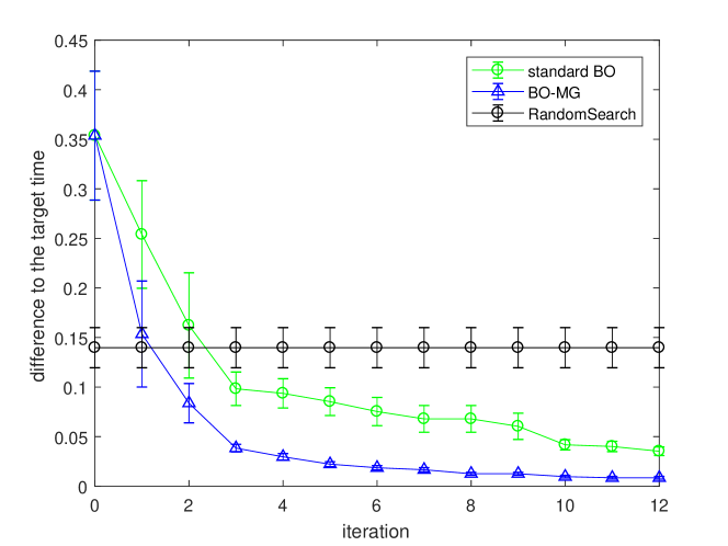
Figure 5: Comparable performance of different algorithms on hyperparameter tuning in neural network. The vertical axis represents the difference to the pre-set test time.

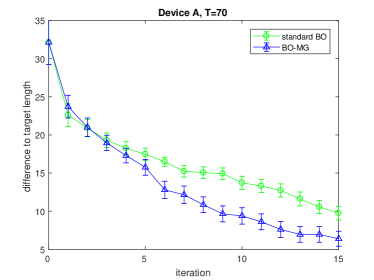
(a)

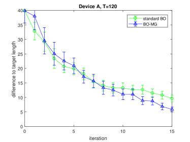
(b)

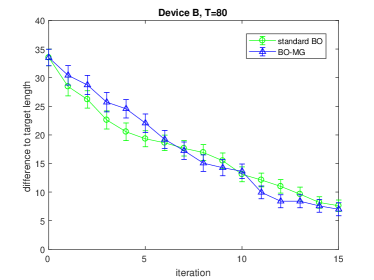
(c)

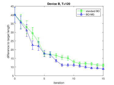
(d)

Figure 6: Optimization of Short Polymer Fibre with specified target lengths: BO-MG vs standard BO. The vertical axis represents the difference from target length $(T)$. Results for Device A are (a)$T=70\mu m$ and (b)$T=120\mu m$; Results for for Device B (c)$T=80\mu m$ and (d)$T=120\mu m$.

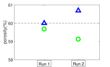
(a)

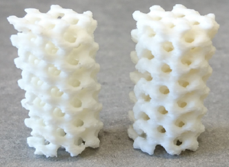
(b)

Figure 7: (a) Optimization of scaffold for a target porosity 60%. Standard BO (circle) vs BO-MG (triangle) Results for two independent runs are shown; (b) 3D printed scaffolds with final BO-MG recommendations: Scaffold porosity 60% (left) and scaffold porosity 50.27% (right).

IV-D Optimization of scaffold with target porosity in 3D printing

With the maturity of 3D printing processes, complex three dimensional porous architectures, or scaffolds, are becoming a favorable feature in a range of product designs applications ranging from topology optimization to tissue engineering structures. Such scaffold structures could not be fabricated by any other form of technology. The ability to derived precise solutions for the overall porosity of a resulting scaffold can be problematic, requiring laborious trial and error based approaches to derive a solution.

Our objective is to derive solution for reduced material consumption when creating a cylindrical structure, with two absolute porosity targets of 50% or 60%. To adjust the porosity, the thickness of the scaffold was adjusted by uniformly projecting the surface outward closing the free volume. This projection was dictated by a design software parameter, named the smallest detail, which has a lower value of 0.05 and can be adjusted in increments of 0.001.

We employ the BO-MG to accelerate scaffold design to achieve the two targeted porosities with fewer number of experiments. We have a hunch that the porosity decreases with the smallest detail. Starting from three random points, we recommended three sequential experiments for targeted porosity 60%. The search range of the smallest detail is between 0.05 and 2. We run this process independently twice and compare the best suggested one from different algorithms. The result for T=60% is shown in Figure 7. BO-MG recommendations are closer to the targeted porosity.

We also exploit all previous experimental results to suggest only one experiment for targeted porosity 50%. The recommended experiment from BO-MG acheives porosity of 50.27% whilst standard BO reaches porosity of 49.22%. The results clearly demonstrate the effectiveness of our method.

V Conclusion

We have proposed a Bayesian optimization algorithm to incorporate the hunches experimenters possess about the change of experimental results with respect to certain variables to accelerate experimental designs. We have explicitly discussed the monotonicity information and how to model it into Bayesian optimization framework. We also provide the regret bound for our method to demonstrate its convergence. The experimental results show that the proposed algorithm significantly outperforms the standard Bayesian optimization and it reduces significant cost in real world applications. Regarding the future work we seek a smart way to automatically detect the trends of the function so that BO strategies can switch freely between different trends. More broadly we have envisaged the benefit of the use of monotonicity information in Bayesian optimization and exploring the use of other types of prior knowledge is a promising direction for efficient experimental design.
Acknowledgment: This research was partially funded by the Australian Government through the Australian Research Council (ARC). Prof Venkatesh is the recipient of an ARC Australian Laureate Fellowship (FL170100006)

References

- [1] E. Brochu, V. M. Cora, and N. De Freitas, “A tutorial on Bayesian optimization of expensive cost functions, with application to active user modeling and hierarchical reinforcement learning,” arXiv preprint arXiv:1012.2599, 2010.
- [2] N. Srinivas, A. Krause, S. Kakade, and M. Seeger, “Gaussian process optimization in the bandit setting: No regret and experimental design,” in ICML, 2010.
- [3] P. V. Balachandran, D. Xue, J. Theiler, J. Hogden, and T. Lookman, “Adaptive strategies for materials design using uncertainties,” in Scientific reports, 2016.
- [4] V. Nguyen, S. Rana, S. K. Gupta, C. Li, and S. Venkatesh, “Budgeted batch bayesian optimization,” in ICDM, Spain, 2016.
- [5] C. Li, D. Rubin de Celis Leal, S. Rana, S. Gupta, A. Sutti, S. Greenhill, T. Slezak, M. Height, and S. Venkatesh, “Rapid bayesian optimisation for synthesis of short polymer fiber materials,” Scientific Reports, vol. 7, 2017.
- [6] M. Feurer, T. Springenberg, and F. Hutter, “Initializing bayesian hyperparameter optimization via meta-learning,” in Proceedings of the Twenty-Ninth AAAI Conference on Artificial Intelligence, 2015.
- [7] C. Li, S. Gupta, S. Rana, V. Nguyen, S. Venkatesh, and A. Shilton, “High dimensional bayesian optimization using dropout,” in International Joint Conference on Artificial Intelligence, 2017.
- [8] S. Rana, C. Li, S. Gupta, V. Nguyen, and S. Venkatesh, “High dimensional Bayesian optimization with elastic Gaussian process,” in Proceedings of the 34th International Conference on Machine Learning, ser. Proceedings of Machine Learning Research, D. Precup and Y. W. Teh, Eds., vol. 70. International Convention Centre, Sydney, Australia: PMLR, 06–11 Aug 2017, pp. 2883–2891. [Online]. Available: http://proceedings.mlr.press/v70/rana17a.html
- [9] J. Riihimaki and A. Vehtari, “Gaussian processes with monotonicity information,” in Proceedings of the Thirteenth International Conference on Artificial Intelligence and Statistics, vol. 9, 2010, pp. 645–652.
- [10] X. Wang and J. O. Berger, “Estimating shape constrained functions using gaussian processes,” SIAM/ASA Journal on Uncertainty Quantification, vol. 4, no. 1, pp. 1–25, 2016.
- [11] T. Choi and P. J. Lenk, “Bayesian analysis of shape-restricted functions using gaussian process priors,” Statistica Sinica, vol. 27, no. 1, pp. 43–69, 2017.
- [12] J. Wu, M. Poloczek, A. G. Wilson, and P. Frazier, “Bayesian optimization with gradients,” in Advances in Neural Information Processing Systems 30, I. Guyon, U. V. Luxburg, S. Bengio, H. Wallach, R. Fergus, S. Vishwanathan, and R. Garnett, Eds., 2017, pp. 5273–5284.
- [13] M. Jauch and victor pena, “Bayesian optimization with shape constraints,” in Advances in Neural Information Processing Systems 2017 Workshop, 2016.
- [14] M. R. Andersen, E. Siivola, and A. Vehtari, “Bayesian optimization of unimodal functions,” in NIPS workshop on Bayesian optimization, 2017.
- [15] T. Desautels, A. Krause, and J. Burdick, “Parallelizing exploration exploitation tradeoffs in gaussian process bandit optimization,” Journal of Machine Learning Research (JMLR), vol. 15, p. 4053?4103, December 2014.
- [16] C. E. Rasmussen and C. K. I. Williams, Gaussian Processes for Machine Learning. The MIT Press, 2005.
- [17] T. P. Minka, “Expectation propagation for approximate bayesian inference,” in Proceedings of the Seventeenth Conference on Uncertainty in Artificial Intelligence, ser. UAI’01. San Francisco, CA, USA: Morgan Kaufmann Publishers Inc., 2001, pp. 362–369. [Online]. Available: http://dl.acm.org/citation.cfm?id=2074022.2074067
- [18] P. Hennig and C. J. Schuler, “Entropy search for information-efficient global optimization,” J. Mach. Learn. Res., vol. 13, pp. 1809–1837, Jun. 2012.
- [19] A. Krause and C. Guestrin, “Near-optimal nonmyopic value of information in graphical models,” in Proceedings of the Twenty-First Conference on Uncertainty in Artificial Intelligence, ser. UAI’05, 2005, pp. 324–331.
- [20] J. Vanhatalo, J. Riihimäki, J. Hartikainen, P. Jylänki, V. Tolvanen, and A. Vehtari, “Gpstuff: Bayesian modeling with gaussian processes,” J. Mach. Learn. Res., vol. 14, no. 1, pp. 1175–1179, Apr. 2013.
- [21] A. SUTTI, M. Kirkland, P. Collins, and R. GEORGE, “An apparatus for producing nano-bodies,” Sep. 12 2014, wO Patent App. PCT/AU2014/000,204. [Online]. Available: https://www.google.ch/patents/WO2014134668A1?cl=en