Intermediate statistics in thermoelectric properties of solids

Abstract

We study the thermodynamics of a crystalline solid by applying intermediate statistics manifested by $q$-deformation. We based part of our study on both Einstein and Debye models, exploring primarily deformed thermal and electrical conductivities as a function of the deformed Debye specific heat. The results revealed that the $q$-deformation acts in two different ways but not necessarily as independent mechanisms. It acts as a factor of disorder or impurity, modifying the characteristics of a crystalline structure, which are phenomena described by q-bosons, and also as a manifestation of intermediate statistics, the B-anyons (or B-type systems). For the latter case, we have identified the Schottky effect, normally associated with high-Tc superconductors in the presence of rare-earth-ion impurities, and also the increasing of the specific heat of the solids beyond the Dulong-Petit limit at high temperature, usually related to anharmonicity of interatomic interactions. Alternatively, since in the q-bosons the statistics are in principle maintained the effect of the deformation acts more slowly due to a small change in the crystal lattice. On the other hand, B-anyons that belong to modified statistics are more sensitive to the deformation.

I Introduction

Studies carried out in the second half of the 20th century have found that under the presence of defects or impurities in a crystal, the electrostatic potential changes its neighborhoods breaking the translational symmetry of periodic potentials and ; ell ; lee . This disturbance can produce electronic wave functions located near the impurity failing to propagate through the crystal. The process of inserting impurities made out of known elements in a semiconductor is called doping.

In this paper, we apply the $q$-deformation in solids to act as defects or impurities, especially in Einstein and Debye solids bri ; bri1 ; bri2 ; bri3 . Our results show that the $q$-deformation parameter modifies the thermodynamic quantities such as entropy, specific heat, and other characteristics of chemical elements zim .

Much researches on $q$-deformation through quantum groups and quantum algebras have been developed in several fields of physics, such as cosmology and condensed matter lei ; che ; ien ; ler ; fuc ; wil ; bie ; mac ; sin ; rpv ; chai ; col ; sou ; lav5 ; bri5 ; Marinho:2019zny ; Marinho:2019zny2 . Even in the absence of a universally recognized satisfactory definition of a quantum group, all the present proposals suggest the idea of deforming a classical object which may be, for example, an algebraic group or a Lie group. In such proposals, the deformed objects lose the group property.

In the literature we also find intermediate or fractional statistics describing anyons aro ; sen ; ach ; fiv ; per ; dal ; nar ; lav ; man ; rov ; free ; aba ; sid ; cla ; Morier , which are one of the versions of nonstandard quantum statistics gen ; gre ; pol ; lav1 as well as non-extensive statistics tsa . As we shall see, the results revealed that $q$-deformation acts in two different ways but not necessarily as independent mechanisms: it acts as a factor of disorder or impurity, modifying the characteristics of a crystalline structure, which are phenomena described by q-bosons, and also as a manifestation of intermediate statistics, the B-anyons (or B-type systems).

The statistical mechanics of anyons have been studied in two spatial dimensions using a natural distinction existing between boson-like and fermion-like anyons wil . Anyons also manifest in any dimensions, including “spinon” excitations in one-dimensional antiferromagnets, as shown long ago by Haldane haldane . Fractional statistics determined by the relation defining permutation symmetry in the many-body wave function

$$\psi(x_{1},\cdots x_{j}\cdots x_{i}\cdots,x_{n})=\exp(i\pi\alpha)\psi(x_{1},\cdots x_{j}\cdots x_{i}\cdots,x_{n}),$$ (1)

where the statistics determining parameter $\alpha$ is a real number, may interpolate between bosons and fermions. The limits $\alpha=0,1$ correspond, respectively, to bosons and fermions. From the literature, we know that the permutation symmetry is related to rotations in two spatial dimensions. In the present study, we shall focus both on the formulation of the intermediate statistics for bosons (B-anyons) and q-bosons associated with the $q$-deformed algebra. The thermal and electrical conductivities and other thermodynamic quantities will be investigated in both cases.

The paper is organized as follows. In Sec. II we introduce the $q$-deformed algebra and develop the intermediate statistics. In Sec. III we apply the intermediate statistics in the Einstein and Debye solid models in three dimensions. The Sec. IV is devoted to our final comments.

II The Algebra of Interpolating Statistics

In order to investigate boson-like interpolating statistics we shall first examine the $q$-deformed algebra defined by

$$bb^{\dagger}-qb^{\dagger}b=q^{-N},\qquad 0\leq q\leq 1,$$ (2)

in terms of creation and annihilation operators $b^{\dagger}$ and $b$, respectively, and quantum number $N$. The regime $q=1$ corresponds to the Bose-Einstein limit. We also add the following relations

$$[N,b]=-b,\qquad[N,b^{\dagger}]=b^{\dagger},\qquad[N]=b^{\dagger}b,\qquad[N+1]=q[N]+q^{-N},$$ (3)

where the basic number $[N]$ is defined as erns

$$[N]=\frac{q^{{N}}-q^{-{N}}}{q-q^{-{1}}}.$$ (4)

On the other hand, one may transform the $q$-Fock space into the configuration space (Bargmann holomorphic representation) flo as in the following:

$$b^{\dagger}=x,\qquad\qquad b=\partial_{x}^{q},$$ (5)

where $\partial_{x}^{q}$ is the Jackson derivative (JD) jac given by

$$\partial_{x}^{q}f{(x)}=\frac{f{(qx)}-f{(q^{-1}x)}}{x{(q-q^{-1})}}.$$ (6)

Note that it becomes an ordinary derivative as $q\to 1$. Therefore, JD naturally occurs in quantum deformed structures. It turns out to be a crucial role in $q$-generalization of thermodynamic relations lav1 . The $q$-Fock space spanned by the orthonormalized eigenstates $|n\rangle$ is constructed according to

$${|n\rangle}=\frac{(b^{\dagger})^{n}}{\sqrt{[n]!}}{|0\rangle},\qquad\qquad b{|0\rangle}=0,$$ (7)

where the basic factorial is given by $[n]!=[n][n-1][n-2]\cdots 1$, with $n$ corresponding to any integer. The actions of the operators $b$, $b^{\dagger}$ and $N$ on the states $|n\rangle$ in the $q$-Fock space are well-known and read

$$b^{\dagger}{|n\rangle}=[n+1]^{1/2}{|n+1\rangle},$$ (8)

$$b{|n\rangle}=[n]^{1/2}{|n-1\rangle},$$ (9)

$$N{|n\rangle}=n{|n\rangle}.$$ (10)

II.1 $q$-bosons

To calculate the $q$-deformed occupation number $n_{i}$ for a boson-like statistics, we start with the Hamiltonian of quantum harmonic oscillators bie ; mac ; nar ; ach ; lav ; wil

$${\cal H}=\sum_{i}{(E_{i}-\mu)}{N_{i}}=\sum_{i}{(E_{i}-\mu)}{b_{i}^{\dagger}b_{i}},$$ (11)

where $\mu$ is the chemical potential. This $q$-deformed Hamiltonian depends implicitly on $q$ through the number operator defined in Eqs. (3)-(4).

Next, we consider the expectation value,

$$[n_{i}]=\frac{\exp\Big{(}-\beta(E_{i}-\mu)\Big{)}tr\Bigg{(}\exp\Big{(}-\beta\displaystyle\sum_{n_{j}}{(E_{j}-\mu)n_{j}b_{i}b_{i}^{\dagger}}\Big{)}\Bigg{)}}{tr\Bigg{(}\exp\Big{(}-\beta\displaystyle\sum_{n_{j}}{(E_{j}-\mu)n_{j}}\Big{)}\Bigg{)}},$$ (12)

the definition $b_{i}b_{i}^{\dagger}=[1+n_{i}]$, and use the cyclic property of the trace to find

$$[n_{i}]=\exp(-\beta(E_{i}-\mu))[1+n_{i}]\,\,\rightarrow\,\,\frac{[n_{i}]}{[1+n_{i}]}=z\exp(-\beta E_{i}),$$ (13)

where $z=\exp(\beta\mu)$ is the fugacity. Proceeding further, we obtain the equation for the $q$-deformed occupation number

$$n_{i}^{(q)}=\frac{1}{2\ln(q)}\ln\left(\frac{z^{-1}\exp(\beta E_{i})-q^{-1}}{z^{-1}\exp(\beta E_{i})-q}\right).$$ (14)

Interesting enough, alternatively, as a consequence of the $q$-deformed algebra, we can also obtain (14) by using the JD because we can formally write the total number of $q$-deformed particles in the form

$$N^{q}=zD_{z}^{q}\ln{\Xi}\equiv\displaystyle\sum_{i}{n_{i,q}},$$ (15)

where $D_{z}^{q}$ is a $q$-deformed differential operator defined as

$$D_{z}^{q}=\frac{q-q^{-1}}{2\ln{q}}\partial_{z}^{q},\qquad\mbox{when\>\> $q\to 1,$}\qquad D^{q}_{z}\to\frac{\partial}{\partial z},$$ (16)

and $\ln\Xi$ defines the undeformed grand-partition function.

II.2 B-anyons

Let us now get a distribution function for B-anyons (or B-type systems). For this, we will expand the Eq. (14) in the the following power series

$$n_{i}^{(q)}=\frac{1}{y}+\left(\frac{1}{6y}+\frac{\overline{q}}{2y^{2}}+\frac{1}{3y^{3}}\right)\varepsilon^{2}+\cdots,$$ (17)

where $y=\exp(\eta)-\overline{q}$, $\eta=\beta(E_{i}-\mu)$ and $\overline{q}=1-\varepsilon$, with $\varepsilon\ll 1$. Taking the leading term we find

$$n_{i}^{(q)}=\frac{1}{y}=\frac{1}{z^{-1}\exp(\beta E_{i})-\overline{q}}.$$ (18)

Now by simple inspection of Eq. (15), analogously, but using ordinary derivative instead of JD, we can write the logarithm of $\overline{q}$-deformed grand-partition function $\Xi_{q}$ as

$$\ln{\Xi_{q}}=-\displaystyle\sum_{i}{\overline{q}^{-1}\ln{\left[1-\overline{q}z\exp(-\beta E_{i})\right]}}.$$ (19)

In the next section, we will deepen our study of solid models by introducing the results obtained in the present section to the energy spectrum in three dimensions, as we can also see in, e.g., rov ; free . We should warn the reader that, we shall refer $\bar{q}$-deformation to B-anyons and $q$-deformation to q-bosons, throughout the remainder of this paper.

III Implementation of Interpolating Statistics

III.1 Deformed Einstein solid

We can consider the solid in contact with a thermal reservoir at temperature $T$, where we have $n_{j}$ labeling the $j$-th oscillator. Given a microscopic state $\{n_{j}\}=\{n_{1},n_{2},\ldots,n_{N}\}$, the energy of this state can be written as

$$E\{n_{j}\}=\displaystyle\sum_{j=1}^{3N}{\hbar\omega_{E}\left(n_{j}+\frac{1}{2}\right)},$$ (20)

where $\omega_{E}$ is the Einstein characteristic frequency. Now substituting the Eq. (20) into Eq. (19), we can determine a $\overline{q}$-deformed Helmholtz free energy per oscillator given by

$$f_{q}\!=\!-\frac{1}{\beta}\displaystyle\lim_{N\to\infty}\frac{1}{N}\ln\Xi_{q}=\frac{\kappa_{B}T}{\overline{q}}\ln(1-\alpha_{q}),\qquad\alpha_{q}=\overline{q}\exp\left(-\frac{\theta_{E}}{T}\right),$$ (21)

where $\beta={1}/{\kappa_{B}T}$, $\kappa_{B}$ is the Boltzmann constant and $\theta_{E}$ is the Einstein temperature defined as $\theta_{E}={\hbar\omega_{E}}/{\kappa_{B}}$. For later use, it is useful to define a $\overline{q}$-deformed Einstein function $E(\alpha_{q})$ as

$$E(\alpha_{q})=\frac{\alpha_{q}}{\overline{q}}\left(\frac{\theta_{E}}{T(\alpha_{q}-1)}\right)^{2}.$$ (22)

In the following, we shall find several important thermodynamic quantities. Firstly, by using the result of Eq. (21) we can determine the specific entropy

$$s_{q}=-\frac{\partial f_{q}}{\partial T}=-\frac{\kappa_{B}}{\overline{q}}\left[\ln(1-\alpha_{q})-\frac{\theta_{E}\alpha_{q}}{T(1-\alpha_{q})}\right],$$ (23)

and the $\overline{q}$-deformed specific heat can be now determined and given by

$$c_{Vq}(T)=T\left(\frac{\partial s_{q}}{\partial T}\right)=\frac{\kappa_{B}\alpha_{q}}{\overline{q}}\left(\frac{\theta_{E}}{T(\alpha_{q}-1)}\right)^{2}.$$ (24)

The specific heat of the Einstein solid as a function of $E(\alpha_{q})$, defined in Eq. (22), can be given as follows

$$c_{Vq}(T)=3\kappa_{B}E(\alpha_{q}).$$ (25)

The complete behaviors are depicted in Figs. 1 and 2 for q-bosons and B-anyons, respectively. In the former case, one should note that when $T\gg\theta_{E}$, with $\theta_{E}$, e.g., around $100K$ for common crystals, one recovers the classical result $c_{Vq}\to 3\kappa_{B}$ when $q=1$, known as the Dulong-Petit law. On the other hand, for sufficiently low temperatures, where $T\ll\theta_{E}$, the specific heat goes exponentially with temperature patt as

$$c_{Vq}\rightarrow\kappa_{B}\left(\frac{\theta_{E}}{T}\right)^{2}\exp\left(-\frac{\theta_{E}}{T}\right).$$ (26)

However, as well-known, at sufficiently low temperatures, the specific heat of the solids does not follow experimentally the exponential function given in Eq. (26). Thus, the undeformed Einstein model recovers the usual specific heat of the solids only at high temperatures.

As for the $\overline{q}$-deformed case, Fig. 2, as the temperature is increased, we notice that the green and blue curves (greater presence of the $\bar{q}$-deformation) present a very different behavior from the red curve (where $\overline{q}=1$). Thus, let us now explore this new picture for B-anyons. The point is that at large temperatures the specific heat becomes

$$c_{Vq}(T)\simeq 3\kappa_{B}\left(\frac{\theta_{E}}{T}\right)^{2}\frac{1}{\Big{(}(\bar{q}-1)-\bar{q}\left(\frac{\theta_{E}}{T}\right)\Big{)}^{2}}=3\kappa_{B}\left(\frac{\theta_{E}}{T}\right)^{2}\frac{1}{\left(\varepsilon+\left(\frac{\theta_{E}}{T}\right)\right)^{2}}.$$ (27)

In the last step we have rewritten the equation in terms of the definition of $\bar{q}=1-\varepsilon$ and $\varepsilon\ll 1$ given in subsection (II.2). Notice that the specific heat always goes to zero as $T\gg\theta_{E}$ for $\bar{q}<1$. This is precisely a consequence of the harmonic oscillator spectrum in Eq. (20) submitted to the B-anyons statistics in Eq. (19). Alternatively, one could also consider the undeformed Bose-Einstein statistics to the spectrum (20) with ${\bar{q}\,}^{n}$ degenerescence for each $n$-th state. Such degenerescence could be associated with interactions among oscillators in contrast with the original Einstein consideration of $3N$ independent harmonic oscillators describing the solid. Thus, the present intermediate statistics could capture realistic interactions even though one previously assumes independent oscillators. Another possibility could be the existence of extra degrees of freedom with same energy quantum number that could be probed by the B-anyons statistics. Finally, the most revealing fact is that the specific heat behaves as the specific heat of a two level system with a maximum at $T\sim\theta_{E}$, that is the well-known Schottky effect, and since it was previously assumed an infinite number of states, such an apparent discrepancy clearly can be seen as an effect of a changing of states counting that may be well understood in terms of the intermediate statistics. This ‘apparent mismatch’ of number of states can be indeed related to impurities. For instance, it has been reported long ago YBACO that some different samples of the YBaCuO high-$T_{c}$ superconductor presented Schottky effect in the specific heat due to the presence of heavy rare-earth-ion impurities.

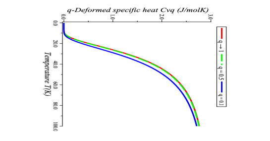
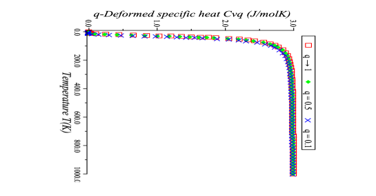
Figure 1: $q$-deformed specific heat $c_{V_{q}}$ vs temperature $T$ in the following intervals: ($T=0-0.1K$) (left), ($T=0-100K$) (center) and ($T=0-1000K$) (right). See Ref. bri .

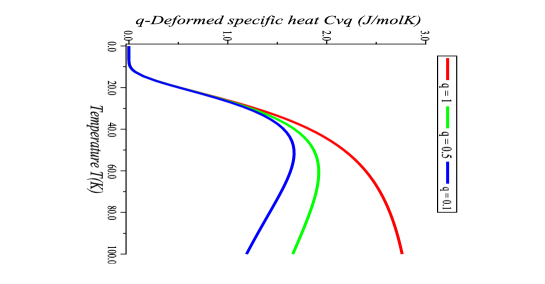
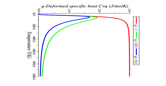
Figure 2: ${\overline{q}}$-deformed specific heat $c_{V_{q}}$ vs temperature $T$ in the following intervals: ($T=0-0.1K$) (left), ($T=0-100K$) (center) and ($T=0-1000K$) (right).

III.2 Deformed Debye solid

Corrections of the Einstein model are given by the Debye model allowing us to integrate out a continuous spectrum of frequencies up to the Debye frequency $\omega_{D}$, giving the total number of normal vibrational modes hua ; patt ; reif ; sal ; kit

$$\int_{0}^{\omega_{D}}g(\omega)d\omega=3N,$$ (28)

where $g(\omega)d\omega$ denotes the number of normal vibrational modes whose frequency is in the range $(\omega,\omega+d\omega)$. The energy expected value of the Planck oscillator with frequency $\omega_{s}$ for the B-anyons statistics is

$$<E_{s}>=\frac{\hbar\omega_{s}}{\exp\left(\frac{\hbar\omega_{s}}{\kappa_{B}T}\right)-\bar{q}}.$$ (29)

To obtain the number of photons between $\omega$ and $\omega+d\omega$, one makes use of the volume in a region on the phase space patt , which results

$$g(\omega)d\omega\approx\frac{2V}{h^{3}}\left[4\pi\left(\frac{\hbar\omega}{c}\right)^{2}\left(\frac{\hbar d\omega}{c}\right)\right]=\frac{V\omega^{2}d\omega}{\pi^{2}c^{3}}.$$ (30)

We now apply the $\overline{q}$-deformation in the same way as in Eq. (25), that means

$$c_{V_{q}}(T)=3\kappa_{B}D(\alpha_{0_{q}}),$$ (31)

where $D(\alpha_{0_{q}})$ is the $\bar{q}$-deformed Debye function that we are going to find shortly. Firstly let us define the function

$$D(\alpha_{0})=\frac{3}{\alpha_{0}^{3}}\int_{0}^{\alpha_{0}}\frac{\alpha^{4}\exp{\alpha}}{[\exp(\alpha)-\bar{q}]^{2}}\;d\alpha,\qquad\alpha_{0}=\frac{\hbar\omega_{D}}{\kappa_{B}T}=\frac{\theta_{D}}{T},$$ (32)

with $\omega_{D}$ and $\theta_{D}$ being the Debye characteristic frequency and temperature, respectively. To perform the integration, it is convenient to make the following change of variable

$$\alpha_{0_{q}}=\frac{\alpha_{0}-\ln(\overline{q})}{\overline{q}}.$$ (33)

Consequently, with this change we obtain as a result of the integration

$$D(\alpha_{0_{q}}) = \frac{{\alpha_{0_{q}}}}{\rm a_{0_{q}}-1}+\frac{12}{({\overline{q})}^{4}\alpha_{0_{q}}^{3}}\Bigg{\{}\frac{\ln{({\overline{q})}^{4}}}{4}+\ln{({\overline{q})}^{3}}\ln\Bigg{(}\frac{\overline{q}-1}{\overline{q}}\Bigg{)}-3\ln{({\overline{q})}^{2}}\rm{Li_{2}}\Bigg{(}\frac{1}{\overline{q}}\Bigg{)}-$$ (34)

$$- 6\ln{({\overline{q})}}\rm{Li_{3}}\Bigg{(}\frac{1}{{\overline{q}}}\Bigg{)}-6\rm{Li_{4}}\Bigg{(}\frac{1}{\overline{q}}\Bigg{)}-\frac{({\overline{q})}^{4}}{4}\;\alpha_{0_{q}}^{4}+({\overline{q})}^{3}\alpha_{0_{q}}^{3}\ln(1-a_{0_{q}})+$$

$$+ 3({\overline{q})}^{2}\alpha_{0_{q}}^{2}\rm{Li_{2}}(a_{0_{q}})-6({\overline{q})}\alpha_{0_{q}}\rm{Li_{3}}(a_{0_{q}})+6\rm{Li_{4}}(a_{0_{q}})\Bigg{\}},$$

where a${}_{0_{q}}=\exp(\alpha_{0_{q}}-\ln(\overline{q}))$ and

$$\rm{Li_{n}(z)}=\displaystyle\sum_{k=0}^{\infty}{\frac{z^{k}}{k^{n}}},$$ (35)

is the polylogarithm function.

Two important limits are discussed in order. For $\alpha_{0_{q}}\ll 1$, the function $D(\alpha_{0_{q}})$ can be expressed in terms of the parameter of the intermediate statistics

$$D(\alpha_{0_{q}})=\frac{\ln(\overline{q})}{(\overline{q})-1}+\frac{\alpha_{0_{q}}}{1-(\overline{q})}\;(13+\ln(\overline{q}))+\cdots$$ (36)

such that at high temperature, $T\gg\theta_{D}$, the corresponding specific heat is

$$c_{V_{q}}\to 3\kappa_{B}\;\frac{\ln(\overline{q})}{(\overline{q})-1}.$$ (37)

Here we can see that the specific heat of the solid behaves asymptotically larger than $3\kappa_{B}$ as $\bar{q}<1$, which means it is effectively going beyond the Dulong-Petit limit at high temperature, a phenomenon that may be related to anharmonicity of interatomic interactions beyond and looks to be probed through B-anyons statistics.

On the other hand, for $\alpha_{0_{q}}\gg 1$, we can write the $\bar{q}$-deformed Debye function (34) as

$$D(\alpha_{0_{q}})\approx\frac{4\pi^{4}}{5{[(\overline{q})\alpha_{0_{q}}]^{3}}}.$$ (38)

Thus, as in the usual Debye solid, at low temperature, $T\ll\theta_{D}$, the specific heat in a $\bar{q}$-deformed Debye solid is proportional to $T^{3}$, due to phonon excitation, a fact that is in agreement with experiments. In addition, we express the $\bar{q}$-deformed specific heat at low temperatures as follows

$$c_{V_{q}}=\frac{1944}{[(\overline{q})\alpha_{0_{q}}]^{3}}\frac{J}{molK}.$$ (39)

In the following we shall explore the $\bar{q}$-deformed (and $q$-deformed) thermal and electrical conductivities which are related with their corresponding undeformed form given by bri

$$\kappa_{q}=\kappa\frac{c_{V_{q}}}{c_{V}}\qquad\qquad\mbox{and}\qquad\qquad\sigma_{q}=\sigma\frac{\kappa_{q}}{\kappa}.$$ (40)

Element	$c_{V_{q}}^{(a)}$			$\kappa_{q}^{(b)}$			$\sigma_{q}^{(c)}$
	$\overline{q}$=1	$\overline{q}$=0.5	$\overline{q}$=0.1	$\overline{q}$=1	$\overline{q}$=0.5	$\overline{q}$=0.1	$\overline{q}$=1	$\overline{q}$=0.5	$\overline{q}$=0.1
Rb	3.0$\times 10^{5}$	2.9$\times 10^{3}$	126	0.58	5.6$\times 10^{(-3)}$	2.4$\times 10^{(-4)}$	8.0$\times 10^{4}$	764	34
Pb	4.5$\times 10^{4}$	1.7$\times 10^{3}$	104	0.35	1.3$\times 10^{(-2)}$	8.0$\times 10^{(-4)}$	4.8$\times 10^{4}$	1.8$\times 10^{3}$	110
Bi	3.1$\times 10^{4}$	1.5$\times 10^{3}$	99	0.08	3.9$\times 10^{(-3)}$	2.5$\times 10^{(-4)}$	8.6$\times 10^{3}$	415	27
Au	1.2$\times 10^{4}$	1.0$\times 10^{3}$	84	3.17	0.27	2.3$\times 10^{(-2)}$	4.6$\times 10^{5}$	4.0$\times 10^{4}$	3.3$\times 10^{3}$
Pt	3.8$\times 10^{3}$	584	65	0.72	0.11	1.2$\times 10^{(-2)}$	9.6$\times 10^{4}$	1.5$\times 10^{4}$	1.6$\times 10^{3}$
Y	2.4$\times 10^{3}$	452	57	0.17	0.03	4.1$\times 10^{(-3)}$	1.7$\times 10^{4}$	$3.2\times 10^{3}$	408
Mn	762	698	124	0.08	2.3$\times 10^{(-2)}$	4.1$\times 10^{(-3)}$	7.0$\times 10^{3}$	2.0$\times 10^{3}$	362
Ti	708	228	41	0.46	0.14	2.5$\times 10^{(-2)}$	2.3$\times 10^{4}$	6.9$\times 10^{3}$	1.2$\times 10^{3}$
Fe	506	168	34	0.80	0.27	5.3$\times 10^{(-2)}$	1.0$\times 10^{5}$	3.4$\times 10^{4}$	6.8$\times 10^{3}$
Rh	475	161	33	1.5	0.51	0.10	2.1$\times 10^{5}$	7.1$\times 10^{4}$	$1.4\times 10^{4}$
Os	420	148	31	0.88	0.31	7.0$\times 10^{(-2)}$	1.1$\times 10^{5}$	3.9$\times 10^{4}$	8.1$\times 10^{3}$
Ru	243	100	24	1.17	0.48	0.12	1.4$\times 10^{5}$	5.5$\times 10^{4}$	1.4$\times 10^{4}$
Cr	210	89	23	0.94	0.40	0.10	7.8$\times 10^{4}$	3.3$\times 10^{4}$	8.5$\times 10^{3}$
Be	18	12	5	2.00	1.33	0.62	3.1$\times 10^{5}$	2.1$\times 10^{5}$	9.5$\times 10^{4}$

Table 1: Chemical elements and their respective specific heat ^a$\left(\frac{J}{molK}\right)$, thermal conductivity ^b$\left(\frac{W}{cm\dot{K}}\right)$, electrical conductivity ^c$(ohm\cdot cm)$, for $T=300K$ and deformed values for $\overline{q}=0.5$ and $\overline{q}=0.1$ kit .

In the Tab. 1 we present the specific heat, thermal and electrical conductivity for some chemical elements, after application of the deformation. We have the undeformed case ($q=1$ for $q$-bosons or $\bar{q}=1$ for B-anyons), a strong deformation case ($\bar{q}=0.1$) and an intermediate case ($\bar{q}=0.5$). For illustration purposes, we choose iron (Fe) and chromium (Cr), which are two materials that can be employed in many scientific areas of interest.

We can observe the behavior of the specific heat of the iron (Fe) (green curve in Fig. 3), as a function of the deformation parameter, starting from the case without deformation ($Fe_{Bulk}$, i.e., when $\overline{q}=1$). As the parameter $\overline{q}$ is acting we notice that this curve reaches the specific heat of other elements, such as the osmium (Os) when $\overline{q}\approx 0.9$ and the $Cr_{Bulk}$ at $\overline{q}\approx 0.58$. For the sake of comparison, in Fig. 4, is shown the behavior for q-bosons, which asymptotically is completely different from the B-anyons case. Whereas in the former case the curves tend to overlap for large $q$ (small deformation), in the latter case the curves tend to overlap for small $\bar{q}$ (large deformation). As expected, since they depend linearly with the specific heat, the deformed thermal and electrical conductivities, follows similar behavior, as shown in Figs. 5 and 6, i.e., the curves degenerate at opposite deformation limits depending on the case involved: q-bosons or B-anyons. We also emphasize the overlap clearly shown in Fig. 5 of the deformed electrical conductivity curves (right) that starts at $\overline{q}\approx 0.62$. On the other hand, we plot in the Figs. 7 and 8 the behavior of the thermal conductivity of deformed chromium (as in enriched or doped samples kit ) as a function of temperature. It is possible to verify that as the temperature increases the behavior of the curves becomes similar, but they overlap more slowly for B-anyons, Fig. 7, than for q-bosons, Fig. 8, as expected according to our previous discussions.

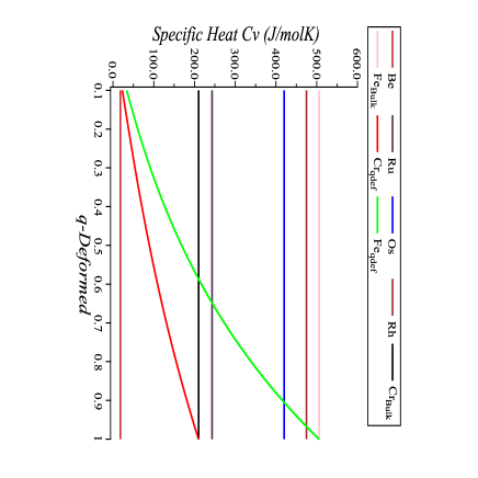
Figure 3: Specific heat $c_{V_{\bar{q}}}$. The Fe and Cr are varying functions of $\overline{q}=0.1$ to $\overline{q}=1$.

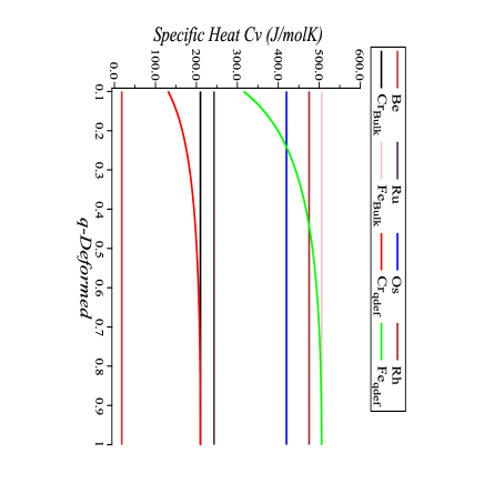
Figure 4: Specific heat $c_{V_{q}}$. The Fe and Cr are varying functions of $q=0.1$ to ${q}=1$. See Ref. bri .

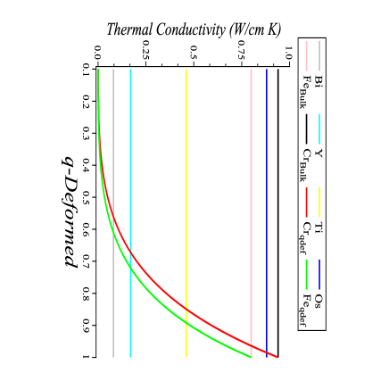
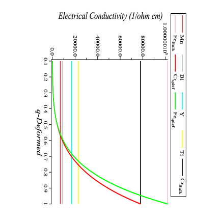
Figure 5: Thermal conductivity $\kappa_{\bar{q}}$. The Fe and Cr are varying functions of $\overline{q}=0.1$ to $\overline{q}=1$, (left). Electrical conductivity $\sigma_{\bar{q}}$. The Fe and Cr are varying functions of $\overline{q}=0.1$ to $\overline{q}=1$ (right).

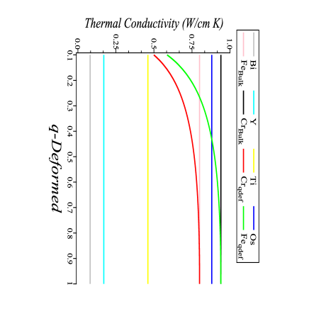
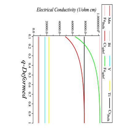
Figure 6: Thermal conductivity $\kappa_{q}$. The Fe and Cr are varying functions of ${q}=0.1$ to ${q}=1$, (left). Electrical conductivity $\sigma_{q}$. The Fe and Cr are varying functions of ${q}=0.1$ to ${q}=1$ (right). See Ref. bri .

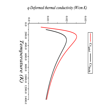
Figure 7: $\bar{q}$-Deformed thermal conductivity $\kappa_{\bar{q}}$ for $\rm Cr_{Bulk}$ ($\bar{q}=1$) and $\rm Cr_{qdef}$ ($\bar{q}=0.1$) as a function of temperature in the interval $T=0$ to $T=1600K$.

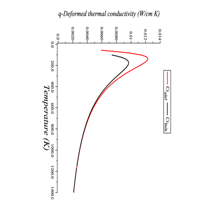
Figure 8: q-Deformed thermal conductivity $\kappa_{q}$ for $\rm Cr_{Bulk}$ ($q=1$) and $\rm Cr_{qdef}$ ($q=0.1$) as a function of temperature in the interval $T=0$ to $T=1600K$. See Ref. bri .

IV Conclusions

The results allow us several important observations. One of them is the fact that in the $q$-deformation there is a region of larger values of the $q$ parameter (less deformed regime) in which different curves of thermal (or electrical) conductivities coincide, that is, the curves degenerate much faster than in the case of B-anyons and vice versa — on the other side, i.e., in the region of small values of $\bar{q}$ the curves of thermal or electrical conductivities degenerate approaching zero. This leads to completely different behaviors. Alternatively, since in the q-bosons the statistics are in principle maintained, the effect of the deformation acts more slowly due to a small change in the crystal lattice. On the other hand, B-anyons belong to modified statistics and are more sensitive to the deformation. Of course, the case of study will decide for one or another deformation type, according to several corresponding situations that we have previously presented. For instance, in the B-anyons case, smaller values of $\bar{q}$, i.e., large deformations, implies a larger asymptotic value of the specific heat as stated in Eq. (37), which involves physics beyond the Dulong-Petit limit, a phenomenon that may be related to anharmonicity of interatomic interactions beyond and looks to be probed through B-anyons statistics. One should further discuss other points around these issues elsewhere.

Our results show that the scenarios with $\overline{q}$ (or $q$)-deformation develop an interesting mechanism that can be associated with factors that modify certain characteristics of the chemical elements. These situations may be related to doping or enrichment of the material in which are inserted certain impurities. Finally, the present study could provide us with a nice theoretical investigation, where many thermodynamic quantities of the material would be calculated and analyzed before application of any experimental techniques.

- (1) P.W. Anderson, Absence of diffusion in certain random lattices, Phys. Rev. 5, 109 (1958).
- (2) R.J. Elliott et al., Rev. Mod. Phys., 3 46 (1974).
- (3) P.A. Lee, T.V. Ramakrishnan, Rev. Mod. Phys. 2, 57 (1985).
- (4) A.A. Marinho, F.A. Brito, C. Chesman, Physica A 391, 3424-3434 (2012).
- (5) D. Tristant, F.A. Brito, Physica A 407, 276-286 (2014).
- (6) A.A. Marinho, F.A. Brito, C. Chesman, J. Phys. Conf. Series 568, 012009 (2014).
- (7) A.A. Marinho, F.A. Brito, C. Chesman, Physica A 443, 324-332 (2016).
- (8) J.M. Ziman, Electron and Phonons - The Theory of Transport Phenomena in Solids, Oxford Univ. Press, (1960).
- (9) J. M. Leinaas and J. Myrheim, Nuovo Cimento B 37, 1 (1977).
- (10) S.S. Chern, et al., Physics and Mathematics of Anyons, World Scientific, Singapore, (1991).
- (11) R. Iengo, K. Lechener, Phys. Reports 213, 179-269 (1992).
- (12) A. Lerda and S. Sciuto, Nucl. Phys. B 401, 613 (1993).
- (13) J. Fuchs, Affine Lie Algebras and Quantum Groups, Cambridge University Press (1992).
- (14) F. Wilczek, Fractional Statistics and Anyon Superconductivity, World Scientific, Singapore, (1990).
- (15) L.C. Biedenharn, M.A. Lohe, Quantum Group Symmetry and -Tensor Algebras, World Scientific, Singapore, (1995).; L.C. Biedenharn, J. Phys. A: Math. Gen. 22, L873 (1989).
- (16) A. Macfarlane, J. Phys. A: Math. Gen. 22, 4581 (1989).
- (17) R. Jaganathan and S. Sinha, J. Phys. Pramana, 3, 64, (2005).
- (18) R. Pharthasarathy, K.S. Viswanathan, J. Phys. A: Math. Gen. 24, 613-617 (1991).
- (19) M. Chaichian, R. Gonzales Felipe, C. Montonen, J. Phys. A: Math. Gen. 26, 4017 (1993).
- (20) L.P. Colatto, J.L. Matheus-Valle, J. Math. Phys. 37, 6121 (1996).
- (21) J. de Souza, E.M.F. Curado, M.A.R. Monteiro, J. Phys. A: Math. Gen. 39, 10415-10425 (2006).
- (22) G. Gervino, A. Lavagno, D. Pigato, J. Phys. Conf. Series 306, 012070 (2011).
- (23) F.A. Brito, A.A. Marinho, Physica A 390, 2497-2503 (2011); A.A. Marinho, F.A. Brito, C. Chesman, Physica A 411, 74-79 (2014); A.A. Marinho, F.A. Brito, J. Math. Phys. 60, 012102 (2019).
- (24) A. A. Marinho and F. A. Brito, arXiv:1904.07843 [cond-mat.stat-mech].
- (25) A. A. Marinho and F. A. Brito, arXiv:1906.00340 [cond-mat.stat-mech].
- (26) D. Arovas, R. Schrieffer, F.Wilczek, and A. Zee, Nucl. Phys. B 251, 117 (1985).
- (27) D. Sen, Nucl. Phys. B 360, 397-408 (1991).
- (28) R. Acharya and P. Narayana Swamy, J. Phys. A 27, 7247-7263 (1994); R. Acharya and P. Narayana Swamy, J. Phys. A 37, 2527 (2004).
- (29) P. N. Swamy, Int. J. Mod. Phys. B 20, 697-713 (2006).
- (30) A. Lavagno, P.N. Swamy, Physica A 389, 993-1001 (2010);
- (31) A. Rovenchak, Low Temp. Phys. 35, 400 (2009); A. Rovenchak, Phys. Rev. A. 89, 052116 (2014); A. Rovenchak, Eur. Phys. J. B 87, 175 (2014).
- (32) M. Freedman, M.B. Hastings, C. Nayak and X.L. Qi, Phys. Rev B. 84, 245119 (2011).
- (33) D. I. Fivel, Phys. Rev. Lett. 65, 3361 (1990).
- (34) W. A. Perkins, Int. J. Theor. Phys. 41, 823 (2002).
- (35) S. L. Dalton and A. Inomata, Phys. Lett. A 199, 315 (1995).
- (36) F. Mancarella, A. Trombettoni and G. Mussardo, Nucl. Phys. B 867, 950-976 (2013).
- (37) A. Algin, M. Senay, Phys. Rev. E. 85, 041123 (2012); A. Algin, M. Senay, Phys. Lett. A. 377, 1797-1803 (2013); A. Algin, A.S. Arikan, E. Dil, Physica A 416, 499-517 (2014); A. Algin, D. Irk and G. Topcu, Phys. Rev. E. 91, 062131 (2015); A. Algin, M. Senay, Physica A 447, 232-246 (2016); A. Algin and A.S. Arikan, J. Stat. Mech., 043105 (2017); A. Algin and A. Olkun, Annals of Phys. 383, 239-256 (2017).
- (38) S.C. Morampudi, A.M. Turner, F. Pollmann, F. Wilczek, Phys. Rev. Lett. 118, 227201 (2017).
- (39) D. Clarke, J.D. Sau, S.D. Sarma, Phys. Rev B. 95, 155451 (2017).
- (40) S. M.-Genoud and V. Ovsienko, arXiv:1812.00170v2 [math.CO].
- (41) G. Gentile, Nuovo Cimento 17, 493 (1940).
- (42) H. S. Green, Phys. Rev. 90, 270 (1953).
- (43) A. P. Polychronakos, Phys. Lett. B 365, 202 (1996).
- (44) A. Lavagno and N.P. Swamy, Phys. Rev. E 61, 1218 (2000); A. Lavagno and N.P. Swamy, Phys. Rev. E 65, 036101 (2002).
- (45) C. Tsallis, J. Stat. Phys. 52, 479 (1988).
- (46) F. D. M. Haldane, Phys. Rev. Lett. 67, 937 (1991).
- (47) E.I. Andritsos et al, J. Phys.: Cond. Matt 25, 235401 (2013).
- (48) T. Ernst, The History of -calculus and a new method. (Dep. Math., Uppsala Univ. 1999-2000).
- (49) E.G. Floratos, J. Phys. Math. 24, 4739 (1991).
- (50) F. Jackson, Mess. Math. 38, 57 (1909).
- (51) R.K. Patthria, Statistical Mechanics, Pergamon press, Oxford (1972).
- (52) S.J. Collocott, R. Driver, L. Dale and S.X. Dou, Phys. Rev. B 37, 7917(R) (1988).
- (53) K. Huang, Statistical Mechanics, John Wiley & Sons, (1987).
- (54) F. Reif, Fundamentals of statistical and thermal physics, Tokyo, (1965).
- (55) S.R.A. Salinas, Introduction to Statistical Physics, Springer-Verlag, NY (2001)
- (56) C. Kittel, Introduction to Solid State Physics, John Wiley & Sons, (1996).