Algebraic cluster models calculations for shape phase transitions of boson-fermion systems

Abstract

The Algebraic Cluster Model(ACM) is an interacting boson model that gives the relative motion of the cluster configurations in which all vibrational and rotational degrees of freedom are present from the outset. We schemed a solvable extended transitional Hamiltonian based on affine ${{SU(1,1)}}$ Lie algebra within the framework for two-, three- and four- body algebraic cluster models that explains both regions $O(4)\leftrightarrow U(3)$, $O(7)\leftrightarrow U(6)$ and $O(10)\leftrightarrow U(9)$, respectively . We offer that this method can be used to study of $k\alpha+x$ nucleon structures with k = 2, 3,4 and x = 1, 2, . . . , in specific x = 1,2 such as structures ${}^{9}Be$,${}^{9}B$,${}^{10}B$ ; ${}^{13}C$, ${}^{13}N$, ${}^{14}N$; ${}^{17}O$, ${}^{17}F$. Numerical extraction to the energy levels, the expectation value of boson number operator and behavior of the overlap of the ground-state wave function within the control parameters of this evaluated Hamiltonian are presented. The effect of the coupling of the odd particle to an even-even boson core is discussed along the shape transition and, in particular, at the critical point.

I 1.Introduction

Algebraic models are advantageous in the many-body and in few-body systems. In algebraic models energy eigenvalues and eigenvectors are obtained by diagonalizing a finite-dimensional matrix, rather than by solving a set of coupled differential equations in coordinate space. As an example, we assign the interacting boson model (IBM), which has been very prosperous in the appositive of the collective states in nuclei 1 . Its dynamical symmetries correspond to the quadrupole vibrator, the axially symmetric rotor and the $\gamma$-unstable rotor in a geometrical description. In addition to these special solutions, the IBM can describe the intermediate cases between any of them equally well. The first application of the algebraic approach to the few-body systems was the vibron model 2 , which was recommended to describe the vibrational and rotational excitations in the diatomic molecules. Algebraic methods give an accurate view to spectroscopic studies and focus on their’s symmetries and selection rules to categorize the basis states, and to evaluate matrix elements of physical observables 3 . The binding energy per nucleon for the light nuclei shows large oscillations with the nucleon number with maxima for nuclei with A =4n and Z=N, especially for the nuclei $\mathrm{{}^{4}He}$, $\mathrm{{}^{8}Be}$, $\mathrm{{}^{12}C}$ and $\mathrm{{}^{16}O}$ for n =1, 2, 3 and 4 respectively, which provides a strong indication of the importance of $\alpha$ clustering in these nuclei 4 . The common method is to introduce a $U(\nu+1)$ spectrum generating algebra for a bound-state problem with $\nu$ degrees of freedom in which all states are assigned to the symmetric representation $[N]$ of $U(\nu+1)$ 5 ; 6 . For the $\nu=5$ quadrupole degrees of freedom in collective nuclei this led to the introduction of the $U(6)$ interacting boson model 1 . Similarly, the $U(4)$ vibron model was proposed to describe the dynamics of the $\nu=3$ dipole degrees of freedom of the relative motion of the two objects, e.g. two atoms in a diatomic molecule 2 , the two clusters in a nuclear cluster model 7 ; 8 ; 9 , or a quark and antiquark in a meson 10 ; 11 . An application to the three-body system involves the six degrees of freedom of the two relative vectors which in the algebraic approach leads to a $U(7)$ spectrum generating algebra 12 ; 13 as an extension of the vibron model. The $U(7)$ model was developed originally to describe the relative motion of the three constituent quarks in baryons 12 ; 13 , but it has also found applications in molecular physics 14 ; 15 and nuclear physics ($\mathrm{{}^{12}C}$ as a cluster of three a particles) 4 ; 5 . The algebraic cluster for the four-body systems in terms of a $U(10)$ spectrum-generation algebra was introduced in 15 . An application to the cluster states in $\mathrm{{}^{16}O}$ suggested that these can be interpreted in terms of rotations and vibrations of tetrahedral configuration of α particles. The triangular configuration in $\mathrm{{}^{12}C}$ and tetrahedral configuration in $\mathrm{{}^{16}O}$ implied by the observed rotational sequence, were confirmed by a study of BE(L) electric transitions along the ground state bands 4 ; 5 ; 16 . In 17 $\mathrm{{}^{8}Be}$, $\mathrm{{}^{12}C}$ and $\mathrm{{}^{16}O}$ nuclei were considered by using an infinite-dimensional algebraic method based on the affine ${{SU(1,1)}}$ Lie algebra for the transitional descriptions of the vibron model and $\alpha$-cluster model. The cluster structures with addition of nucleons discussed especially in the Be isotopes with a variety of methods 17 ; 18 ; 19 ; 20 ; 21 ; 22 ; 23 ; 24 ; 25 ; 26 ; 27 ; 28 ; 29 ; 30 . In Ref 31 ; 32 , single-particle levels in cluster potentials in $k\alpha+x$ nucleon structures within the framework of a cluster shell model (CSM) calculated. In nuclear physics s-orbit and p-orbit adjaceny achived by studying in light nuclei as we see in carbon isotopes 18 . Hafstad and Teller studied (4n + 1) nuclei, e.g. ${}^{9}Be$, ${}^{13}C$ and ${}^{17}O$. Their ideas were based upon the structure of the ${}^{5}He$ nucleus in which the last neutron was in a p-orbit 18 ; 21 ; 22 .

The study of the quantum phase transitions enjoys a substantial interest in the algebraic models of the nuclear structure. There is mutual relations between shapes (phases) and dynamic symmetry limits. The analytical solutions provide a process in which the system undergoes a change from one dynamical symmetry to another one. The first examples 33 ; 34 were related to the Interaction Boson Model Approximation (IBA) 1 and the Vibron model 1 ; 3 .

The aim of this contribution is to discuss the quantum phase transitions in the algebraic cluster models for the two-, three- and four- body cluster, to transition description in $U(3)\leftrightarrow O(4)$, $U(6)\leftrightarrow O(7)$ and $U(9)\leftrightarrow O(10)$. This model can be solved by using an infinite dimensional algebraic technique in the IBM framework. This method was applied to the $k\alpha+x$ nucleon structures consisting of $k$ $\alpha$-particles and $x$ nucleons, such as structures ${}^{9}Be$,${}^{9}B$,${}^{10}B$ ; ${}^{13}C$, ${}^{13}N$, ${}^{14}N$; ${}^{17}O$ and ${}^{17}F$, corresponding to the exchange of neutrons and $\alpha$-particles. In order to describe the phase transition, we calculate some observables such as energy level, level crossing, expectation values of boson number operator and overlap of the ground-state wave function. The results of calculations for these nuclei are presented and are compared with the corresponding experimental data. In this work ,the role of a fermion with angular momentum j at the critical point on quantum phase transitions in bosonic systems is investigated.

The specific aims of the present study and the structure of this paper are as follows: In section 2, we introduce the algebraic cluster model, followed by a discussion of the permutation symmetry. Section 3 briefly summarizes the theoretical aspects of the model. Numerical results are presented in section 4 and section 5 is devoted to summarize and to justify some conclusion.

II The algebraic cluster model (ACM)

In this section, we introduce the algebraic cluster model. It is based on the spectrum generating algebra of $U(\nu+1)$, where $\nu=3(n-1)$ represents the number of the relative spatial degrees of freedom. As special cases the ACM contains the $U(4)$ vibron model 2 for the two-body problems $(n=2)$, the $U(7)$ model 12 ; 13 ; 15 ; 4 ; 5 for three-body clusters $(n=3)$ and the $U(10)$ model 16 ; 35 ; 36 for four-body clusters $(n=4)$.

The relevant degrees of freedom of a system of n-body clusters are given by the $n-1$ relative Jacobi coordinates

$$\vec{\rho}_{k}=\frac{1}{\sqrt{k(k+1)}}(\sum_{i=1}^{k}\vec{r}_{i}-k\vec{r}_{k+1})\quad\quad k=1,2,...,n-1$$ (1)

and their conjugate momenta. Here $\vec{r}_{i}$ denotes the position vector of the $i-th$ cluster (i=1,2,…,n).

Instead of a formulation in terms of coordinates and momenta, the method of bosonic quantization is used which consists of introducing a dipole boson with $L_{P}=1^{-}$ for each independent relative coordinate and an auxiliary scalar boson with $L_{P}=0^{+}$

$$s^{\dagger},b_{k,m}^{\dagger}$$ (2)

with $k=1,...,n-1$ and $m=−1,0,1$. The scalar boson does not represent an independent degree of freedom, but is added under the restriction that the Hamiltonian commutes with the number operator

$$N=s^{\dagger}s+\sum_{k}\sum_{m}b_{k,m}^{\dagger}b_{k,m}$$ (3)

i.e. the total number of bosons $N=n_{s}+\sum_{k}n_{k}$ is conserved. The set of $〖(3n-2)〗^{2}$ bilinear products of creation and annihilation operators spans the Lie algebra of $U(3n-2)$.

In this contribution, we study the ACM for identical clusters which is relevant to $\alpha$-cluster nuclei such as $\mathrm{{}^{8}Be}$, $\mathrm{{}^{12}C}$ and $\mathrm{{}^{16}O}$. For these systems, the Hamiltonian has to be invariant under the permutation group $S_{n}$. The permutation symmetry of n identical objects is determined by the transposition $P(12)$ and the cyclic permutation $P(12...n)$ 37 . All other permutations can be expressed in terms of these two elementary ones. The transformation properties under $S_{n}$ of all operators in the model originate from those of the building blocks. The scalar boson, $s^{\dagger}$, transforms as the symmetric representation $[n]$, whereas the dipole Jacobi bosons, $b_{k}^{\dagger}$ with $k=1,...,n-1$ transform as the $n-1$ components of the mixed symmetry representation $[n-1,1]$.

Hamiltonian that describes the relative motion of a system of n identical clusters, and is a scalar under the permutation group $S_{n}$ and is rotationally invariant. It conserves the parity as well as the total number of bosons, as given by

$$H=\epsilon_{0}s^{\dagger}\tilde{s}-\epsilon_{1}\sum_{i}b^{\dagger}\tilde{b}+u_{0}s^{\dagger}s^{\dagger}\tilde{s}\tilde{s}-u_{1}\sum_{k}s^{\dagger}b_{k}^{\dagger}s^{\dagger}\tilde{b}_{k}+\nu_{0}(\sum_{k}b_{k}^{\dagger}\tilde{b}_{k}\tilde{s}\tilde{s}+hc)+\sum_{L}\sum_{ijkl}\nu^{(L)}_{ijkl}[b_{i}^{\dagger}\times b_{j}^{\dagger}]^{(L)}[\tilde{b}_{k}\times\tilde{b}_{l}]^{(L)}$$ (4)

with $\tilde{b}_{k,m}={(-1)}^{(1-m)}b_{k,-m}$ and $\tilde{s}=s$ by construction, the $\epsilon_{0}$, $\epsilon_{1}$, $u_{0}$, $u_{1}$ and $\nu_{0}$ terms in Equation (4) are invariant under $S_{n}$.

In this contribution, we consider two dynamical symmetries of the ACM Hamiltonian for the n-body problem which are related to the group lattice

$$U(3n-2)\supset\{^{U(3n-3)}_{O(3n-2)}\supset O(3n-3)$$

which are called the $U(3n-3)$ and $SO(3n-2)$ limits of the ACM, respectively. A geometric analysis shows that the $U(3n-3)$ limit corresponds for large N to the (an)harmonic oscillator in $3(n-1)$ dimensions and the $SO(3n-2)$ limit to the deformed oscillator in $3(n-1)$ dimensions 35 ; 36 .

III Theoretical framework

Algebraic models provide elegant and simple paradigms for the behavior of a wide variety of physical systems. The basic idea of algebraic models is that Hamiltonians and other physical operators of these systems can be realized by using a set of boson operators, since the collective excitations of these systems can be regarded as a set of interacting bosons. The spectrum of the systems can be generated by an appropriate unitary Lie algebra, called spectrum generating algebra. Dynamical symmetries often play an important role in the approach. There is one to one correspondence between the shapes (phases) and dynamic symmetry limits in which analytical solutions to the model exist. The shape (phase) transition of these models is referred to as a process in which the system undergoes a change from one dynamical symmetry to another one. The method for diagonalization of the Hamiltonian in the transitional region is not as easy as in either of the limits, especially when the dimension of the configuration space is relatively large. To avoid these problems, an algebraic Bethe ansatz method within the framework of an infinite dimensional $SU(1,1)$ Lie algebra has been proposed by Pan et al… 38 ; 39 .

III.1 The $SU(1,1)$ expression of Bethe ansatz equations for two-cluster systems

III.1.1 The odd-A nuclei : ${}^{9}_{4}Be$ and ${}^{9}_{4}B$

For more than two decades, is known that the ${}^{9}_{4}Be$ nucleus is an example of a molecular covalent bond in nuclear physics, Where two particles with valence neutron are limited. The ${}^{9}_{4}Be$ nucleus , which has unlimited system properties $2\alpha+n$ is the “cornerstone” of cluster physics18 ; 21 ; 22 ; 32 . Due to its low neutron separation threshold, separation of ${}^{9}_{4}Be$ can be an origination of astable ${}^{8}_{4}Be$ nuclei. The ${}^{8}_{4}Be$ isotope is known as the only nucleus whose ground state is distinguished as the $\alpha$-particle Bose condensate. A study of the division of the ${}^{9}_{4}Be$ nucleus in $\alpha$-particle pair appears to be a clear starting point than the more complex $N\alpha$-systems. This method can also be used to describe the odd-A nuclei. For example, ${}^{9}_{4}Be$ may be assumed to be composed of two $\alpha$-particles and a valence neutron, forming, at larger $\alpha+\alpha$ separations ${}^{5}He$ nuclei, where the neutron abides in a $p_{3/2}$-orbit. We assume for ${}^{9}Be$ a structure similar to ${}^{9}Be$, with the odd neutron exchanged by an odd-proton18 ; 21 ; 22 ; 32 .

The boson algebraic structure will be always taken to be $\mathrm{U^{B}(4)}$ , while the fermion algebraic structure will depend on the values of the angular momenta, j, taken into consideration 10 . Two possible dynamical symmetry limits, $U^{B}(3)$ and $O^{B}(4)$, are related to the following two algebraic chains,

$$U^{B}(4)\otimes U^{F}(2j+1)\supset\left\{\begin{array}[]{l}{U^{(B)}}(3)\\ {O^{(B)}}(4)\end{array}\right\}\ \otimes SU^{F}(2j+1)\supset O^{B}(3)\otimes Sp^{F}(2j+1)\supset O^{B}(3)\otimes SU^{F}(2)\supset Spin^{BF}(3)$$ (5)

The negative parity states in the odd-mass nuclei ${}^{9}_{4}Be$ and ${}^{9}_{4}B$ are built mainly on the $\mathrm{2p_{\frac{3}{2}}}$ shell model orbit40 . The single - particle orbits $\mathrm{1d_{\frac{5}{2}}}$ and $\mathrm{2s_{\frac{1}{2}}}$ establish the positive parity states in ${}^{9}_{4}Be$ and ${}^{9}_{4}B$ isotopes31 . In this study, a simplifying assumption is made that single particle states are built on the $\mathrm{2p_{\frac{3}{2}}}$ and $\mathrm{2s_{\frac{1}{2}}}$. The lattices of algebras in these cases are obtained by putting j=3/2 and 1/2 in Eq.(5), respectively.

The Lie algebra corresponding to the $SU(1,1)$ group is generated by the operators $S^{x}$ where $x=0$ and $\pm 1$. To extend this model, we introduce the $SU(1,1)$ pairing algebras for s and b bosons as,

$$S^{+}(s)=\frac{1}{2}{s^{\dagger}}^{2}\quad\quad\quad S^{-}(s)=\frac{1}{2}s^{2}\quad\quad\quad S^{0}(s)=\frac{1}{2}(s^{\dagger}s+\frac{1}{2})=\frac{1}{2}n_{s}+\frac{1}{4}$$ (6)

$$S^{+}(b)=\frac{1}{2}{b^{\dagger}}.{b^{\dagger}}\quad\quad\quad S^{-}(b)=\frac{1}{2}\tilde{b}.\tilde{b}\quad\quad\quad S^{0}(b)=\frac{1}{2}(b^{\dagger}\tilde{b}+\frac{3}{2})=\frac{1}{2}n_{b}+\frac{3}{4}$$ (7)

where $n_{s}$ and $n_{b}$ are the number operators for s and b bosons which satisfy the following commutation relations

$$[S^{0},S^{\pm}]=\pm S^{\pm}\quad\quad\quad[S^{+},S^{-}]=-2S^{0}$$ (8)

The Casimir operator of $SU(1,1)$ can be written as

$$C_{2}(SU(1,1))=S^{0}(S^{0}-1)-S^{+}S^{-}$$ (9)

The representation is determined by a single number k. Let us assume that $|k\mu\rangle$ is a basis vector of an irrep of $SU(1,1)$, where κ can be any positive real number, and $\mu=k,k+1,...$. Then

$$C_{2}(SU(1,1))|k\mu\rangle=k(k-1)|k\mu\rangle\quad\quad\quad S^{0}|k\mu\rangle=\mu|k\mu\rangle$$ (10)

Now, we introduce the operators of infinite dimensional $SU^{sb}(1,1)$ algebra similar to what has been defined by Pan et al. in ref. 40 ,

$$S_{n}^{\pm}=c_{s}^{(2n+1)}S^{\pm}(s)+c_{b}^{(2n+1)}S^{\pm}(b)$$ (11)

$$S_{n}^{0}=c_{s}^{2n}S^{0}(s)+c_{b}^{2n}S^{0}(b)$$ (12)

where $c_{s}$ and $c_{b}$ are the real control parameters, and n can be taken to be $1,2,3,...$ . To evaluate the energy spectra and transition probabilities, let us consider $|lw\rangle$ as the lowest weight state of $SU^{sb}(1,1)$ algebra which should satisfy

$$S^{-}(s)|lw\rangle=0\quad\quad\quad S^{-}(b)|lw\rangle=0$$ (13)

The lowest weight states,$|lw\rangle_{sb}$ are actually a set of basis vectors of the chain $U(4)\supset U(3)\supset O(3)\supset O(2)$ which

$$|lw\rangle^{B}_{sb}=|N_{B},k_{s}=\frac{1}{2}(\nu_{s}+\frac{1}{2}),\mu_{s}=\frac{1}{2}(n_{s}+\frac{1}{2}),k_{b}=\frac{1}{2}(L+\frac{3}{2}),\mu_{b}=\frac{1}{2}(n_{b}+\frac{3}{2}),LM\rangle$$ (14)

where $N_{B}=\nu_{s}+\nu_{b}$, $n_{b}=L$, $n_{s}=\nu_{s}=0$ or $1$. Hence, we have

$$S_{n}^{0}|lw\rangle=(c_{s}^{(2n)}S^{⁰}(s)+c_{b}^{(2n)}S^{⁰}(b))|lw\rangle=\Lambda_{n}^{0}|lw\rangle$$ (15)

$$\Lambda_{n}^{0}=(c_{s}^{(2n)}(\nu_{s}+\frac{1}{2})+c_{b}^{(2n)}{(L+\frac{3}{2}))}\frac{1}{2}$$ (16)

The following Hamiltonian for description of negative and positive states in transitional region is prepared

$$\hat{H}=gS_{0}^{+}S_{0}^{-}+\alpha S_{1}^{0}+\beta\hat{C}_{2}(SO^{B}(3))+\gamma\hat{C}_{2}(spin^{BF}(3))$$ (17)

For evaluating the eigenvalue of Hamiltonian Eqs. (17), the eigenstates are considered as

$$|k;\nu_{s}\nu_{b}n_{\Delta}LJM\rangle=\Theta S_{x_{1}}^{+}S_{x_{2}}^{+}S_{x_{3}}^{+}...S_{x_{k}}^{+}|lw\rangle^{BF}$$ (18)

With Clebsch- Gordan (CG) coefficient, we can calculate lowest weight state, $\mathrm{|lw\rangle^{BF}}$, in terms of boson and fermion part as

$$|lw\rangle^{BF}=\sum_{j}\sum_{m_{j}=-j}^{m_{j}=+j}C_{m,m-m_{j},m_{j}}^{J,L,j}|lw\rangle_{sb}^{B}|j,m_{j}\rangle$$ (19)

The $\mathrm{C_{m,m_{L},m_{j}}^{J,L,j}}$symbols represent Clebsch-Gordan coefficients.

$$|lw\rangle^{B}_{sb}=|N_{B},k_{s}=\frac{1}{2}(\nu_{s}+\frac{1}{2}),\mu_{s}=\frac{1}{2}(n_{s}+\frac{1}{2}),k_{b}=\frac{1}{2}(L+\frac{3}{2}),\mu_{b}=\frac{1}{2}(n_{b}+\frac{3}{2}),LM\rangle$$ (20)

$$S_{n}^{0}|lw\rangle=(c_{s}^{(2n)}S^{⁰}(s)+c_{b}^{(2n)}S^{⁰}(b))|lw\rangle=\Lambda_{n}^{0}|lw\rangle$$ (21)

$$\Lambda_{n}^{0}=(c_{s}^{(2n)}(\nu_{s}+\frac{1}{2})+c_{b}^{(2n)}{(L+\frac{3}{2}))}\frac{1}{2}$$ (22)

The eigenvalues of Hamiltonians Eqs. (17) can then be expressed;

$$E^{(k)}=h^{(k)}+\alpha\Lambda_{1}^{0}+\beta L(L+1)+\gamma J(J+1)$$ (23)

where

$$h^{(k)}=\sum_{i=1}^{k}\frac{\alpha}{x_{i}}=\sum_{i=1}^{k}\frac{gc_{s}^{2}(\nu_{s}+\frac{1}{2})}{1-c_{s}^{2}x_{i}}+\frac{gc_{b}^{2}(L+\frac{3}{2})}{1-c_{b}^{2}x_{i}}-\sum_{i\neq j}\frac{2g}{x_{i}-x_{j}}\quad\quad g=1$$ (24)

III.1.2 The odd-odd nuclei : ${}^{10}_{5}B$

The structure of the odd-odd nuclei may be illustrated as an unpaired proton and an unpaired neutron coupled to a boson core. In this paper, the method described in Refs.38 ; 39 will be developed and performed to mixed boson-fermion-fermion systems. The approach based on boson-fermion symmetries has been also applied to odd-odd systems. On the other, IBFM has been increased to odd-odd nuclei, and mention to as IBFFM. To simplify computing, the structure of the odd-odd nuclei is described as an unpaired proton and an unpaired neutron coupled to a ${}^{8}_{4}Be$.

It should be noted that we have investigated the phase transition from rigid to non-rigid shapes in the case that odd proton and odd neutron in j=3/2 configurations coupled to core that undergoes a transition from $U^{B}(3)$ and $O^{B}(4)$ condition.

After this, we considered the state that an unpaired proton and an unpaired neutron being in a j=3/2 shell. The algebraic structure underlying our IBFM-1 approach is shown in Eq.(25).The bosons are initially coupled and so are fermions, and then the compounds of bosons and fermions connect to each other. In Eq.(25) , the chain upper show the state that bosons have $\mathrm{U^{B}(3)}$ dynamical symmetric while bosons in chain lower have $\mathrm{O^{B}(4)}$ dynamical symmetric.

$$U^{B}(4)\otimes(U^{F_{\pi}}(4)\otimes U^{F_{\nu}}(4))\supset\left\{\begin{array}[]{l}{U^{(B)}}(3)\\ {O^{(B)}}(4)\end{array}\right\}\ \otimes SU^{F_{\pi\nu}}(4)\supset O^{B}(3)\otimes Sp^{F_{\pi\nu}}(4)\supset O^{B}(3)\otimes SU^{F_{\pi\nu}}(2)\supset O_{\pi\nu}^{BF}(3)\supset O_{\pi\nu}^{BF}(2)$$ (25)

The Hamiltonian for the odd-odd nuclei may be written as a sum of a boson part and parts describing the residual interaction between boson-fermion and fermion-fermion interaction. The Hamiltonian with $j_{\pi}=\frac{3}{2}$ and $j_{\nu}=\frac{3}{2}$ in transitional region between $\mathrm{U(3)-O(4)}$ limits in terms of the casimir operators of the group chain (Eq.(25)) is prepared

$$\hat{H}=gS_{B,0}^{+}S_{B,0}^{-}+\alpha S_{B,1}^{0}+\beta\hat{C}_{2}(SO^{B}(3))+\rho\hat{C}_{2}(SP^{F_{\pi\nu}}(4))+\delta\hat{C}_{2}(SU^{F_{\pi\nu}}(2))+\gamma\hat{C}_{2}(O^{BF_{\pi\nu}}(3))$$ (26)

Eq.(26) is the suggested Hamiltonian for boson - fermion-fermion systems and $\mathrm{\alpha}$ , $\mathrm{\beta}$ ,$\mathrm{\delta}$, $\mathrm{\rho}$ and $\mathrm{\gamma}$ are real parameters. Hamiltonian Eq.(26) is equivalent to Hamiltonian of rigid limit when $\mathrm{c_{s}=1}$ and with Hamiltonian of non-rigid limit if $\mathrm{c_{s}=0}$ and $\mathrm{c_{b}}\neq 0$. So, the $\mathrm{c_{s}\neq c_{b}\neq 0}$ situation just corresponds to transitional region.

For evaluating the eigenvalues of Hamiltonian Eqs. (26) the eigenstates are considered as 36 ; 37

$$|k;\nu_{s},\nu_{b},(\xi_{1},\xi_{2}),SL,JM\rangle=\Theta S_{x_{1}}^{+}S_{x_{2}}^{+}S_{x_{3}}^{+}...S_{x_{k}}^{+}|lw\rangle^{BF_{\pi\nu}}$$ (27)

$N_{B},\nu_{b},(\xi_{1},\xi_{2}),S,L,JM$ are quantum numbers of $U^{B}(4),O^{B}(4),SP^{F_{\pi\nu}}(4),SU^{F_{\pi\nu}}(2),SO^{B}(3)$, $O^{BF_{\pi\nu}}(3)$ and $O^{BF_{\pi\nu}}(2)$, respectively.

The lowest weight state $\mathrm{|lw\rangle^{BF_{\pi\nu}}}$ is calculated as:

$$|lw\rangle^{BF_{\pi\nu}}=\sum_{m_{\pi}m_{\nu}m_{\pi\nu}M}{C_{m_{\pi\nu},m_{\pi},m_{\nu}}^{J_{\pi\nu},j_{\pi},j_{\nu}}C_{M,m_{\pi\nu},M_{b}}^{J,J_{\pi\nu},L}|j_{\pi},m_{\pi}\rangle|j_{\nu},m_{\nu}\rangle|lw\rangle_{sb}^{B}}$$ (28)

The eigenvalues of Hamiltonian Eq. (26) can then be expressed;

$$E^{(k)}=h^{(k)}+\alpha\Lambda_{1}^{0}+\beta L(L+1)+\rho(\xi_{1\pi\nu}(\xi_{1\pi\nu}+3)+\xi_{2\pi\nu}(\xi_{2\pi\nu}+1))+\delta S(S+1)+\gamma J(J+1))$$ (29)

III.2 The $SU(1,1)$ expression of Bethe ansatz equations for three-cluster systems

III.2.1 The odd-A nuclei : ${}^{13}_{6}C$ and ${}^{13}_{7}N$

Similar to the covalently bound structures of two $\alpha$ particles and neutrons discussed earlier, we can continue the discussion with three $\alpha$ particles and neutrons. To start we can regard to the properties of ${}^{13}C$ for which the experimental evidence has recently been collected 18 ; 31 ; 32 .

The structure of the linear chain configurations for ${}^{13}C$ and ${}^{14}C$ can be based on the $\alpha+^{9-10}Be$ structure. The carbon isotopes provide an excellent example for testing the concept of full spectroscopy, because for these nuclei, different types of reactions have been studied. The structure of ${}^{13}C$ will be examined in more detail; it will serve as an image of the identification of cluster states, which are often particle unstable states. By using a large amount of information a complete spectroscopy of the states can be obtained to stimulate the energy of 20MeV. With a dissociation of the single-particle states the ordering of the remaining states into $K=3/2^{-}$ and $3/2^{+}$ bands is obtained. The mass 13 nuclei is the subject of many shell-model calculations and its sources17 .

Generally, normal (negative) parity states in ${}^{13}C$ (and ${}^{13}N$) arise from various re-couplings of the nine nucleons in the p-shell. For the positive parity states with a nucleon in the sd-shell, a very satisfactory description is obtained in the weak coupling model, with the lowest two core states ${}^{12}C$. The basic positive-parity states of ${}^{13}C$ are obtained by coupling a 2s- or ld-neutron to a core which is either the $0^{+}$ ground or $2^{+}$ first excited state of ${}^{12}C$ and then antisymmetrizing17 . These are states of configuration $1s^{4}1p^{8}2s$ or $1s^{4}1p^{8}1d$; states of configuration $1s^{3}1p^{10}$ are omitted 18 ; 31 ; 32 .

The negative parity states in the even - odd nuclei ${}^{13}_{6}C$ and ${}^{13}_{7}N$ are built mainly on the $\mathrm{1p_{\frac{1}{2}}}$ shell model orbit. The single - particle orbits $\mathrm{1d_{\frac{5}{2}}}$ and $\mathrm{2s_{\frac{1}{2}}}$ establish the positive parity states in odd-mass ${}^{13}_{6}C$ and ${}^{13}_{7}N$ isotopes. In this study, a single particle states are built on the j=1/2. In this case,the boson algebraic structure will be always taken to be $\mathrm{U^{B}(7)}$ coupled to a fermion with angular momentum j=1/2

Two possible dynamical symmetry limits, $U^{B}(6)\otimes U^{F}(2)$ and $O^{B}(7)\otimes U^{F}(2)$, are related to the following two algebraic chains as:

$$U^{B}(7)\otimes U^{F}(2)\supset\left\{\begin{array}[]{l}{U^{(B)}}(6)\\ {O^{(B)}}(7)\end{array}\right\}\ \otimes SU^{F}(2)\supset O^{B}(6)\otimes SU^{F}(2)\supset O^{B}(3)\otimes SU^{F}(2)\supset Spin^{BF}(3)$$ (30)

By employing the generators of Algebra $\mathrm{\widehat{SU(1,1)}}$ and Casimir operators of subalgebras , the following Hamiltonian for transitional region between $U^{B}(6)\otimes U^{F}(2)$ and $O^{B}(7)\otimes U^{F}(2)$ is suggested as

$$\hat{H}=gS_{0}^{+}S_{0}^{-}+\alpha S_{1}^{0}+\beta\hat{C}_{2}(O^{B}(6))+\gamma\hat{C}_{2}(O^{B}(3))+\rho\hat{C}_{2}(spin^{BF}(3))$$ (31)

The eigenvectors of the Hamiltonian for the excitations can be written as

$$|k;\nu_{s}\nu_{b_{1}}\nu_{b_{2}}n_{\Delta}LJM\rangle=\mathcal{N}S_{x_{1}}^{+}S_{x_{2}}^{+}S_{x_{3}}^{+}...S_{x_{k}}^{+}|lw\rangle^{BF}$$ (32)

where

$$|lw\rangle^{BF}=\pm\sqrt{{\frac{L\pm m+\frac{1}{2}}{(2L+1)}}}|lw\rangle_{sb_{1}b_{2},m-\frac{1}{2}}^{B}\chi_{+}+\sqrt{{\frac{L\mp m+\frac{1}{2}}{(2L+1)}}}|lw\rangle_{sb_{1}b_{2},m+\frac{1}{2}}^{B}\chi_{-}$$ (33)

These yield the eigenvalues $E^{(k)}$ of the Hamiltonian Equation (31) in the form

$$E^{(k)}=h^{(k)}+\alpha\Lambda_{1}^{0}+\beta(\nu(\nu+4))+\gamma L(L+1)+\rho J(J+1)$$ (34)

where

$$h^{(k)}=\sum_{i=1}^{k}\frac{\alpha}{x_{i}}=\sum_{i=1}^{k}\frac{gc_{s}^{2}(\nu_{s}+\frac{1}{2})}{1-c_{s}^{2}x_{i}}+\frac{gc_{b_{1}}^{2}(\nu_{b_{1}}+\frac{3}{2})}{1-c_{b_{1}}^{2}x_{i}}+\frac{gc_{b_{2}}^{2}(\nu_{b_{2}}+\frac{3}{2})}{1-c_{b_{2}}^{2}x_{i}}-\sum_{i\neq j}\frac{2g}{x_{i}-x_{j}}\quad\quad g=1$$ (35)

$$\Lambda_{1}^{0}={c_{s}^{2}(\nu_{s}+\frac{1}{2})+c_{b_{1}}^{2}(\nu_{b_{1}}+\frac{3}{2})+c_{b_{2}}^{2}(\nu_{b_{2}}+\frac{3}{2})}$$ (36)

III.2.2 The odd-odd nuclei : ${}^{14}_{7}N$

The ${}^{14}N$ nucleus is considered as a mediator between the cluster nucleus ${}^{12}C$ and the doubly magic nucleus ${}^{16}O$ 17 ; 32 . The study of ${}^{14}N$ nuclei can expand understanding of the evolution of increasingly complex structures beyond the $\alpha$-clustering. The information about the structure of ${}^{14}N$ has practical value. As a major component of the Earth’s atmosphere the ${}^{14}N$ nucleus can be a source of the light rare earth elements Li, Be and B, as well as of deuterium. Production of these elements happens as a result of bombardment of the atmosphere in its lifetime by high energy cosmic particles. Hence, the cluster features of the ${}^{14}N$ fragmentation can define the affluence of lighter isotopes. Beams of ${}^{14}N$ nuclei can be used in radiation therapy, which also gives a applied interest in obtaining detailed data about the characteristics of the ${}^{14}N$ fragmentation 18 ; 31 .

Similar to structures of ${}^{10}_{5}B$ discussed before, the method outlined in Sec.3 will be applied for description of ${}^{14}_{7}N$. The basic positive-parity states of ${}^{14}N$ are obtained by coupling a $1p_{1/2}$-neutron and $1p_{1/2}$-proton to a core that undergoes a transition from $U^{B}(6)$ and $O^{B}(7)$ situation. The lattice of algebras in this case is shown as

$$U^{B}(7)\otimes(U^{F_{\pi}}(2)\otimes U^{F_{\nu}}(2))\supset\left\{\begin{array}[]{l}{U^{(B)}}(6)\\ {O^{(B)}}(7)\end{array}\right\}\ \otimes U^{F_{\pi\nu}}(2)\supset O^{B}(3)\otimes SU^{F_{\pi\nu}}(2)\supset O^{B}(3)\otimes SU^{F_{\pi\nu}}(2)\supset O_{\pi\nu}^{BF}(3)\supset O_{\pi\nu}^{BF}(2)$$ (37)

The Hamiltonian with $j_{\pi}=\frac{1}{2}$ and $j_{\nu}=\frac{1}{2}$ in transitional region between $\mathrm{U(6)-O(7)}$ limits in terms of the casimir operators of the group chain (Eq.(55)) is prepared

$$\hat{H}=gS_{0}^{+}S_{0}^{-}+\alpha S_{1}^{0}+\beta\hat{C}_{2}(O^{B}(6))+\gamma\hat{C}_{2}(O^{B}(3))+\gamma^{\prime}\hat{C}_{2}(SU^{F_{\pi\nu}}(6))+\rho\hat{C}_{2}(spin^{BF}(3))$$ (38)

For evaluating the eigenvalues of Hamiltonian Eqs. (56) the eigenstates Eq.(36) are considered with the lowest weight states,$|lw\rangle_{sb_{1}b_{2}}$.

The eigenvalues of ${}^{14}_{7}N$ odd-odd three-cluster nuclei can then be obtained as;

$$E^{(k)}=h^{(k)}+\alpha\Lambda_{1}^{0}+\beta\nu(\nu+4)+\gamma L(L+1)+\gamma^{\prime}S(S+1)+\rho J(J+1)$$ (39)

III.3 The $SU(1,1)$ expression of Bethe ansatz equations for four-cluster systems

III.3.1 The odd-A nuclei : ${}^{17}_{8}O$ and ${}^{17}_{9}F$

In this work, we study the structure ${}^{17}_{8}O$ as Four -$\alpha$ particles and a neutron and ${}^{17}_{9}F$ as Four -$\alpha$ particles and a proton. The negative parity states in the even - odd nuclei ${}^{17}_{8}O$ and ${}^{17}_{9}F$ are built mainly on the $\mathrm{1p_{\frac{1}{2}}}$ shell model orbit. The single - particle orbits $\mathrm{1d_{\frac{5}{2}}}$ and $\mathrm{2s_{\frac{1}{2}}}$ establish the positive parity states in odd-mass${}^{17}_{8}O$ and ${}^{17}_{9}F$isotopes. In this study, a simplifying assumption is made that single particle states are built on the j=1/2.

In this case,the boson algebraic structure will be always taken to be $\mathrm{U^{B}(10)}$ coupled to a fermion with angular momentum j=1/2

Two possible dynamical symmetry limits, $U^{B}(9)\otimes U^{F}(2)$ and $O^{B}(10)\otimes U^{F}(2)$, are related to the following two algebraic chains as:

$$U^{B}(10)\otimes U^{F}(2)\supset\left\{\begin{array}[]{l}{U^{(B)}}(9)\\ {O^{(B)}}(10)\end{array}\right\}\ \otimes SU^{F}(2)\supset O^{B}(9)\otimes SU^{F}(2)\supset O^{B}(3)\otimes SU^{F}(2)\supset Spin^{BF}(3)$$ (40)

In a four-cluster model, the Hamiltonian for the transitional region between $U^{B}(9)\otimes U^{F}(2)\leftrightarrow O^{B}(10)\otimes U^{F}(2)$ can be considered as

$$H=gS_{0}^{+}S_{0}^{-}+\alpha S_{1}^{0}+\beta C_{2}(O^{B}(9))+\gamma C_{2}(O^{B}(3))+\rho C_{2}(Spin^{BF}(3))$$ (41)

The eigenvalues Equation (41) can be expressed as

$$E^{(k)}=h^{(k)}+\alpha\Lambda_{1}^{0}+\beta(\nu(\nu+7))+\gamma L(L+1)+\rho J(J+1)$$ (42)

$$h^{(k)}=\sum_{i=1}^{k}\frac{\alpha}{x_{i}}=\sum_{i=1}^{k}\frac{gc_{s}^{2}(\nu_{s}+\frac{1}{2})}{1-c_{s}^{2}x_{i}}+\frac{gc_{b_{1}}^{2}(\nu_{b_{1}}+\frac{3}{2})}{1-c_{b_{1}}^{2}x_{i}}+\frac{gc_{b_{2}}^{2}(\nu_{b_{2}}+\frac{3}{2})}{1-c_{b_{2}}^{2}x_{i}}+\frac{gc_{b_{3}}^{2}(\nu_{b_{3}}+\frac{3}{2})}{1-c_{b_{3}}^{2}x_{i}}-\sum_{i\neq j}\frac{2g}{x_{i}-x_{j}}\quad\quad g=1$$ (43)

$$\Lambda_{1}^{0}={c_{s}^{2}(\nu_{s}+\frac{1}{2})+c_{b_{1}}^{2}(\nu_{b_{1}}+\frac{3}{2})+c_{b_{2}}^{2}(\nu_{b_{2}}+\frac{3}{2})+c_{b_{3}}^{2}(\nu_{b_{3}}+\frac{3}{2})}$$ (44)

III.4 The fitting procedure

In order to obtain the numerical results for energy spectra $\mathrm{(E^{(k)})}$ of the considered nuclei , a set of non-linear Bethe-Ansatz equations (BAE) with k- unknowns for k-pair excitations must be solved. To achieve this aim, we have changed variables in two-cluster nuclei as

$$\mathrm{C=\frac{c_{s}}{c_{b}}\leq 1,y_{i}=c_{b}^{2}x_{i}}$$

In addition, the constants of Hamiltonian with the least square fitting processes to experimental data are obtained . A useful and simple numerical algorithm for solving the BAE Equations (24) and for extracting of the constants in comparison with the experimental energy spectra of the considered nuclei is based on using of Matlab software which will be outlined simultaneously. To determine the roots of the BAE with the specified values of $\nu_{s}$ and $\nu_{b}$, we solve Equation (24) with the definite values of C and $\alpha$ for $i=1$ and then we use the function ”syms var” in Matlab to obtain all roots. We then repeat this procedure with different C and $\alpha$ to minimize the root mean square deviation, $\sigma$, between the calculated energy spectra and the experimental counterparts which explore the quality of the extraction processes. The deviation is defined by the equality

$$\sigma=(\frac{1}{N_{tot}}|E_{exp}(i)-E_{cal}(i)|^{2})^{\frac{1}{2}}$$ (45)

$N_{tot}$ is the number of energy levels which are included in the extraction processes. We have extracted the best set of Hamiltonian’s parameters, i.e. $g$, $\alpha$ and $\beta$, via the available experimental data.

Similar to the procedures to extract the parameters of the transitional Hamiltonian in the two-cluster case,Eqs. (35)and (43) were solved for the i = 1 case with definite values C and $\alpha$ in three and four cluster nuclei.

IV Numerical results

This section presents the results of the numerical solution of the phase transition observable of the algebraic cluster model for the two-, three- and four- body clusters such as level crossing, expectation values of the boson numbers and Calculated variation behavior of the overlap of the ground-state wave function. In this research paper, we have taken ${}^{9}Be$,${}^{9}B$,${}^{10}B$ ; ${}^{13}C$, ${}^{13}N$, ${}^{14}N$; ${}^{17}O$, ${}^{17}F$ nuclei for the two-, three- and four- cluster.

IV.1 Energy spectrum and level crossing

In the wake of the theoretical method achieved beforehand, we apply our algebraic model for the cluster model to the ${}^{9}Be$,${}^{9}B$,${}^{10}B$ ; ${}^{13}C$, ${}^{13}N$, ${}^{14}N$; ${}^{17}O$ , ${}^{17}F$ nuclei.

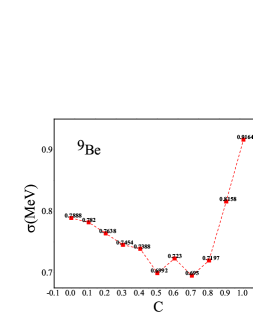
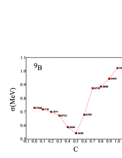
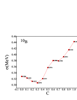
Figure 4: The root mean square deviation as a function of the control parameter C for two-cluster nuclei.

In our calculation, we have proposed the control parameters $C$ values in the 0-1 region for the two-, three- and four- body clusters. So, we have analyzed the properties of the ${}^{9}Be$,${}^{9}B$,${}^{10}B$ ; ${}^{13}C$, ${}^{13}N$, ${}^{14}N$; ${}^{17}O$ and ${}^{17}F$ nuclei in order to investigate the ground- and excited-state spectra related to the models-the best fit which guarantees that the parameters are well determined. Eigenvalues of these models are obtained by solving Bethe Ansatz equations with the extraction processes to experimental data to obtain constants of the Hamiltonian. We explore the best-fitting parameters, which are extracted by the procedures explained in Sect. 3 and the least-square fit to the available experimental data 41 ; 42 ; 43 for the excitation energies for the ${}^{9}Be$,${}^{9}B$,${}^{10}B$ ; ${}^{13}C$, ${}^{13}N$, ${}^{14}N$; ${}^{17}O$ and ${}^{17}F$ nuclei and the ability of the $SU(1,1)$-based transitional Hamiltonian in the reproduction of all considered levels and also the acceptable degree of the extraction procedures.The root mean square deviation, $\sigma$, between the calculated energy spectra and the experimental counterparts as a function of the control parameter C for these nuclei are shown in Figs (4),(5) and (6). Tables 1-8 show the calculated energy spectra along with the experimental values. Our results show that two-cluster nuclei have vibrational features but the gamma-unstable rotor character is dominant while a dominancy of dynamical symmetry O(7) exist for three-cluster nuclei, and the four-cluster nuclei have dominant vibrational features. We see from the figure that in this case the odd particle drives the system toward deformation or sphericity.

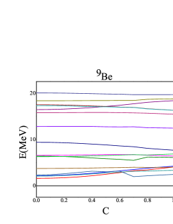
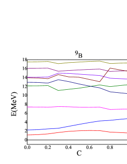
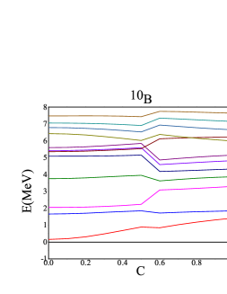
Figure 1: Energy levels as a function of the control parameter C for two-cluster nuclei.

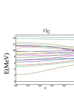
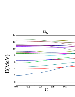
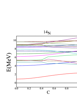
Figure 2: Energy levels as a function of the control parameter C for three-cluster nuclei.

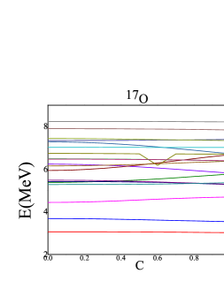
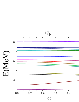
Figure 3: Energy levels as a function of the control parameter C for four-cluster nuclei .

To display how the energy levels change as a function of the control parameter C , the lowest energy levels as a function of C f for the ${}^{9}Be$,${}^{9}B$,${}^{10}B$ ; ${}^{13}C$, ${}^{13}N$, ${}^{14}N$, ${}^{17}O$ and ${}^{17}F$ nuclei are shown in Figs. 1,2 and 3. The figures show how the energy levels as a function of the control parameter C evolve from one dynamical symmetry limit to the other. It can be seen from the figures that numerous level crossings occur.

IV.2 Expectation values of boson number

The other quantal order parameters that we mention here are the expectation values of the boson number operators. The expectation values of $n_{b}$ are the significant objectives of phase transition. So, we calculated these values to show the treatment of phase transition. In order to calculate the expectation values of the b-boson number operator, we have to select the suitable roots. Given the proper amount of roots,, we have calculated $<n_{b}>$ for two, three and four - clusters in even - even and odd-A nuclei.

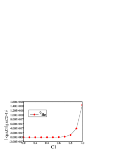
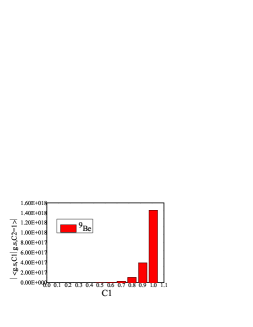
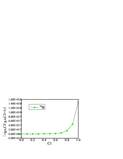
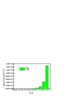
Figure 8: The Calculated variation behavior of the overlap of the ground-state wave function as a function of control parameter C for N=10 .

Fig.8 shows the expectation values of the b-boson number operator for the lowest states even-even (left panel) and odd-A nuclei (right panel) as a function of control parameter for $N=10$ bosons. Fig.9 shows the expectation values of the b-boson number operator for the lowest states even-even nuclei as a function of ${C}$ and ${C_{b}}$ control parameters.

The sudden change in these quantities show the phase transition. Figures show that the expectation values of the number of vector-bosons remain approximately constant for a limit and only begin to change rapidly for the other limit. It can be seen from Fig.8 that in due to the presence of the fermion, the transition is made sharper for even-even nuclei while is made smoother for odd-A nuclei. We also found that the position of the critical point has been shifted by the addition of the odd particle with respect to the even case. As a outcome the behavior of the odd and even systems at the corresponding critical points are rather similar.

IV.3 Calculated variation behavior of the overlap of the ground-state wave function

It has been shown previously that the overlap of the ground-state wave function with that in the dynamical symmetries may also serve as a signature of the phase transition 44 ; 45 ; 46 ; 47 . We have calculated the overlap of the ground-state wave functions of the Hamiltonians (17) and (26) in $\left|{\left\langle{{g.s.{C_{1}}}}\mathrel{\left|{\vphantom{{g.s.{C_{1}}}{g.s.{C_{2}}=1}}}\right.\kern-1.2pt}{{g.s.{C_{2}}}}\right\rangle}\right|$ with $C_{2}=1$ for ${}^{9}_{4}Be$ and ${}^{10}_{5}B$. The obtained results are illustrated in Fig.10. It indicates that the largest absolute value of the derivative of $\left|{\left\langle{{g.s.{C_{1}}}}\mathrel{\left|{\vphantom{{g.s.{C_{1}}}{g.s.{C_{2}}=1}}}\right.\kern-1.2pt}{{g.s.{C_{2}}}}\right\rangle}\right|$ with respect to ${C_{1}}$ occurs around the critical point ${C_{1}}=0.6$ for ${}^{9}_{4}Be$ and ${C_{1}}=0.4$ for ${}^{10}_{5}B$ .

V Conclusion

In this paper, we have studied the phase transitions of the algebraic cluster models. ${}^{9}Be$,${}^{9}B$,${}^{10}B$ ; ${}^{13}C$, ${}^{13}N$, ${}^{14}N$; ${}^{17}O$, ${}^{17}F$ nuclei were studied in the $SU(3)\leftrightarrow SO(4)$, $SU(6)\leftrightarrow SO(7)$ and $SU(9)\leftrightarrow SO(10)$ phase transitions, related to the description of the relative motion of the cluster configurations. A solvable extended transitional Hamiltonian which is based on $SU(1,1)$ algebra is proposed to pave the way for of quantum phase transition between the spherical and the deformed phases. The validity of the presented parameters in the cluster-IBM and cluster-IBFM formulations has been investigated and it is seen that there exists a satisfactory agreement between the presented results and the experimental counterparts. The obtained results in this study confirm that this ACM technique is worth extending for investigating odd-A and odd-odd nuclei. So, the clustering survives the addition of one and two particles. we have presented here a analysis of quantum phase transitions in a system of N bosons and one fermion and shown that the addition of a fermion greatly modifies the critical value at which the phase transition occurs. Our studies confirm the importance of the odd nuclei as necessary signatures to characterize the occurrence of the phase transition and to determine the precise position of the critical point.

Acknowledgements

NA would like to thank Iran National Science Foundation (INSF) for supporting this work financially under the grant No. 97010553. All authors wish to thank the Research Council of University of Tabriz for the grants.

Table 1. Energy spectra for ${{}^{9}Be}$. The experimental values are taken form Ref.43 .

$J^{\pi}$	C=0	C=0.1	C=0.2	C=0.3	C=0.4	C=0.5	C=0.6	C=0.7	C=0.8	C=0.9	C=1	$E_{exp}$
$(3/2)^{-}_{1}$	0	0	0	0	0	0	0	0	0	0	0	0
$(5/2)^{-}_{1}$	1.5889	1.6239	1.7267	1.901	2.1473	2.4758	2.8195	3.2445	3.4093	3.743	4.0505	2.43
$(1/2)^{-}_{1}$	2.1532	2.1897	2.2968	2.4665	2.686	2.943	3.2173	3.5007	3.7879	4.0321	4.25	2.78
$(3/2)^{-}_{2}$	6.5591	6.5716	6.6042	6.6461	6.6831	6.7262	6.7162	6.7302	6.5936	6.4986	6.3929	5.59
$(7/2)^{-}_{1}$	6.4043	6.3726	6.2991	6.1774	6.0107	5.8307	5.6922	5.4697	6.1993	6.146	6.0962	6.38
$(5/2)^{-}_{2}$	9.3756	9.3569	9.282	9.1595	8.9961	8.825	8.6027	8.4211	8.078	7.8513	7.6473	7.94
$(7/2)^{-}_{2}$	12.7982	12.8008	12.8056	12.8112	12.8146	12.741	12.71	12.7323	12.5301	12.4819	12.438	11.28
$(1/2)^{-}_{2}$	16.4439	16.4738	16.5639	16.7055	16.8882	17.1396	17.3836	17.7009	18.0258	18.2294	18.3975	16.97
$(5/2)^{-}_{3}$	17.5033	17.4853	17.4308	17.3415	17.2226	17.1377	16.9803	16.9338	16.6338	16.4517	16.2801	11.81
$(5/2)^{-}_{4}$	18.3618	18.3625	18.3692	18.379	18.3902	18.3977	18.4304	18.4193	18.6775	18.7308	18.7788	14.48
$(1/2)^{+}_{1}$	2.3193	2.3899	2.5843	2.8548	3.1364	3.0205	3.1554	1.9545	2.143	2.3158	2.4537	1.68
$(5/2)^{+}_{1}$	2.0687	2.1038	2.2032	2.3563	2.5456	2.7504	2.941	3.1169	3.1547	3.2556	3.3277	3.05
$(3/2)^{+}_{1}$	3.7176	3.7255	3.7472	3.7798	3.8193	3.8745	3.912	3.9776	3.9447	3.9683	3.9954	4.704
$(9/2)^{+}_{1}$	6.2726	6.2827	6.3102	6.3609	6.4381	6.5235	6.6269	6.7087	6.6292	6.7506	6.8721	6.76
$(5/2)^{+}_{2}$	15.7784	15.7847	15.8014	15.8179	15.8223	15.8264	15.7848	15.7465	15.6724	15.5554	15.4296	16.67
$(7/2)^{+}_{1}$	17.2635	17.2528	17.2193	17.1649	17.0928	17.0477	16.9385	16.9044	16.5922	16.4325	16.274	17.493
$(9/2)^{+}_{2}$	20.0563	20.0434	20.0079	19.9559	19.8958	19.8227	19.7702	19.6737	19.6714	19.6731	19.6896	19.42

Table 2. Energy spectra for ${{}^{9}B}$. The experimental values are taken form Ref.43 .

$J^{\pi}$	C=0	C=0.1	C=0.2	C=0.3	C=0.4	C=0.5	C=0.6	C=0.7	C=0.8	C=0.9	C=1	$E_{exp}$
$(3/2)^{-}_{1}$	0	0	0	0	0	0	0	0	0	0	0	0
$(5/2)^{-}_{1}$	1.1265	1.1913	1.3628	1.6772	1.9321	2.0676	2.1273	2.1008	1.764	1.6621	1.5428	2.36
$(1/2)^{-}_{1}$	2.2418	2.3055	2.4924	2.6239	3.0569	3.4863	3.8993	4.258	4.4005	4.6424	4.8387	2.75
$(7/2)^{-}_{1}$	7.3997	7.3858	7.3512	7.4955	7.4425	7.3368	7.3298	7.354	6.8307	6.9002	6.9699	6.97
$(7/2)^{-}_{2}$	12.1371	12.1504	12.2106	11.0978	11.3742	11.6108	11.9778	12.3512	11.9667	12.2299	12.4531	11.65
$(5/2)^{-}_{2}$	12.9455	12.9026	12.7621	13.5193	13.098	12.5604	12.098	11.6862	10.804	10.5526	10.3495	12.19
$(1/2)^{-}_{2}$	14.0609	14.0776	14.1118	14.983	14.9314	14.76	14.6158	14.4548	13.8505	13.7401	13.6454	14.01
$(3/2)^{-}_{2}$	16.076	16.0852	16.1148	15.4139	15.5923	15.7009	15.8239	15.9048	15.3796	15.4846	15.5471	14.66
$(5/2)^{-}_{3}$	13.9636	13.9107	13.7407	14.6736	14.159	14.078	13.576	13.0789	16.1277	15.6881	15.3283	14.7
$(1/2)^{-}_{3}$	17.5124	17.5339	17.5996	17.1171	17.3408	17.4799	17.6109	17.6833	17.1517	17.2383	17.2808	17.076

Table 3. Energy spectra for ${{}^{10}B}$. The experimental values are taken form Ref.43 .

$J^{\pi}$	C=0	C=0.1	C=0.2	C=0.3	C=0.4	C=0.5	C=0.6	C=0.7	C=0.8	C=0.9	C=1	$E_{exp}$
$3^{+}_{1}$	0	0	0	0	0	0	0	0	0	0	0	0
$1^{+}_{1}$	0.1583	0.1976	0.3104	0.4811	0.6846	0.892	0.8499	1.0251	1.1804	1.3127	1.4227	0.718
$0^{+}_{1}$	1.6624	1.675	1.7101	1.7587	1.809	1.851	1.7166	1.761	1.7957	1.8247	1.852	1.74
$1^{+}_{2}$	2.0485	2.054	2.0723	2.107	2.1615	2.2366	3.0838	3.1261	3.1794	3.2401	3.3043	2.154
$2^{+}_{1}$	3.7534	3.7669	3.8042	3.8557	3.9098	3.9572	3.6231	3.7107	3.7825	3.836	3.8713	3.587
$3^{+}_{2}$	5.0882	5.089	5.0932	5.1039	5.1243	5.1547	4.1825	4.2161	4.2547	4.2941	4.3309	4.774
$2^{+}_{2}$	5.4188	5.4261	5.4485	5.4854	5.5349	5.5925	4.5908	4.6551	4.7182	4.776	4.826	5.164
$1^{+}_{3}$	5.5978	5.6099	5.6456	5.7014	5.7713	5.847	4.8667	4.952	5.0309	5.0999	5.1571	5.18
$2^{+}_{3}$	5.3566	5.3647	5.3889	5.4279	5.4789	5.536	6.1214	6.1627	6.193	6.2107	6.2167	5.92
$4^{+}_{1}$	6.427	6.4064	6.3463	6.2538	6.1399	6.0183	6.381	6.2598	6.1517	6.0602	5.9862	6.025
$3^{+}_{3}$	6.785	6.7739	6.7406	6.6858	6.6127	6.5273	6.9328	6.8535	6.7771	6.7079	6.6484	7.002
$2^{+}_{4}$	7.0534	7.0496	7.0362	7.0098	6.9672	6.909	7.3467	7.2988	7.2462	7.1937	7.1451	7.469
$0^{+}_{2}$	7.4772	7.4788	7.4809	7.4774	7.4619	7.4309	7.7467	7.7284	7.7013	7.6698	7.6377	7.56

Table 4. Energy spectra for ${{}^{13}C}$. The experimental values are taken form Ref.44 .

$J^{\pi}$	C=0	C=0.1	C=0.2	C=0.3	C=0.4	C=0.5	C=0.6	C=0.7	C=0.8	C=0.9	C=1	$E_{exp}$
$(1/2)^{-}_{1}$	0	0	0	0	0	0	0	0	0	0	0	0
$(3/2)^{-}_{1}$	5.281	5.3013	5.3618	5.4611	5.597	5.7661	5.9635	6.1827	6.4158	6.6536	6.8868	3.684507
$(5/2)^{-}_{1}$	6.2531	6.2745	6.3371	6.4364	6.5662	6.7186	6.8854	7.0576	7.2263	7.3832	7.5217	7.549
$(1/2)^{-}_{2}$	8.3267	8.3351	8.3585	8.3917	8.4277	8.4591	8.4792	8.4826	8.466	8.4278	8.3693	8.858
$(3/2)^{-}_{2}$	7.7344	7.7524	7.8055	7.891	8.0048	8.1418	8.2965	8.463	8.6351	8.8065	8.9716	9.899
$(7/2)^{-}_{1}$	9.6398	9.6437	9.6558	9.6771	9.7087	9.7513	9.8046	9.8673	9.9365	10.0087	10.0799	10.753
$(5/2)^{-}_{2}$	8.7064	8.7255	8.7807	8.8663	8.9739	9.0943	9.2185	9.3379	9.4456	9.5363	9.6066	6.864
$(1/2)^{-}_{3}$	11.523	11.5102	11.4715	11.4067	11.3158	11.1993	11.0588	10.8971	10.7185	10.5284	10.3334	12.140
$(3/2)^{-}_{3}$	11.5842	11.5728	11.5371	11.4731	11.3757	11.2407	11.0654	10.8499	10.5974	10.3146	10.0109	11.748
$(5/2)^{-}_{3}$	12.5563	12.546	12.5124	12.4484	12.3449	12.1933	11.9873	11.7248	11.408	11.0443	10.6458	12.130
$(7/2)^{-}_{2}$	14.5464	14.5322	14.4922	14.433	14.3652	14.2984	14.2425	14.2056	14.1932	14.2079	14.2495	12.438
$(9/2)^{-}_{1}$	13.8813	13.8717	13.8437	13.8002	13.7453	13.6838	13.6208	13.5617	13.5118	13.4756	13.4559	13.410
$(1/2)^{+}_{1}$	2.1693	2.2375	2.433	2.7366	3.115	3.5363	3.9701	4.3911	4.7793	5.1207	5.407	3.086
$(5/2)^{+}_{1}$	4.7845	4.8133	4.897	5.0284	5.1971	5.3914	5.5998	5.8116	6.0174	6.2094	6.3818	3.85
$(5/2)^{+}_{2}$	6.9698	6.9933	7.0612	7.1676	7.3034	7.4589	7.6244	7.7916	7.9534	8.1045	8.2411	6.86
$(7/2)^{+}_{1}$	6.9782	6.9827	6.9969	7.0228	7.0625	7.1172	7.1866	7.2688	7.36	7.4558	7.5514	7.492
$(3/2)^{+}_{1}$	6.8121	6.8379	6.9099	7.013	7.1275	7.2342	7.3175	7.6375	7.3797	7.3543	7.2953	7.677
$(3/2)^{+}_{2}$	8.9975	8.9956	8.9911	8.9865	8.9855	8.9916	9.0073	9.0331	9.0679	9.1094	9.1547	8.25
$(9/2)^{+}_{1}$	9.7626	9.7462	9.6996	9.6297	9.5459	9.4575	9.3729	9.2986	9.2394	9.1981	9.1757	9.499.8
$(1/2)^{+}_{2}$	10.0908	11.0819	11.0531	10.9997	10.9167	10.8009	10.6524	10.474	10.2709	10.0503	9.8201	10.996
$(7/2)^{+}_{2}$	11.3489	11.3426	11.3253	11.3011	11.2752	11.2523	11.2359	11.2287	11.2319	11.2459	11.2701	11.848
$(5/2)^{+}_{3}$	12.1396	12.1218	12.0642	11.9574	11.7913	11.559	11.2628	10.9059	10.4998	10.0585	9.5982	11.950

Table 5. Energy spectra for ${{}^{13}N}$. The experimental values are taken form Ref.44 .

$J^{\pi}$	C=0	C=0.1	C=0.2	C=0.3	C=0.4	C=0.5	C=0.6	C=0.7	C=0.8	C=0.9	C=1	$E_{exp}$
$(1/2)^{-}_{1}$	0	0	0	0	0	0	0	0	0	0	0	0
$(3/2)^{-}_{1}$	3.91493	3.9237	3.9501	3.9944	4.0569	4.1373	4.2349	4.3484	4.4758	4.6144	4.7612	3.509
$(5/2)^{-}_{1}$	6.4094	6.4245	6.4679	6.5344	6.6163	6.7051	6.7924	6.8712	6.9364	6.9848	7.0152	7.387
$(1/2)^{-}_{2}$	8.8234	8.8198	8.8089	8.7896	8.7609	8.7218	8.6717	8.6102	8.5372	8.4531	8.3585	8.92
$(3/2)^{-}_{2}$	8.5307	8.5384	8.5597	8.5895	8.6204	8.6447	8.6555	8.6481	8.6207	8.5736	8.5097	9.52
$(5/2)^{-}_{2}$	11.0251	11.0257	11.02667	11.0258	11.0197	11.0055	10.9806	10.9437	10.8947	10.8341	10.7636	10.35
$(7/2)^{-}_{1}$	10.6842	10.674	10.6446	10.5988	10.5409	10.4759	10.4085	10.3431	10.2833	10.2319	10.1905	10.36
$(5/2)^{-}_{3}$	10.973	10.9741	10.9762	10.9758	10.9683	10.949	10.9137	10.8599	10.7865	10.694	10.5843	9.83
$(3/2)^{-}_{3}$	12.277	12.2696	12.2456	12.2075	12.1575	12.0987	12.0336	11.9644	11.8919	11.8162	11.7366	11.87
$(7/2)^{-}_{2}$	12.3174	12.315	12.3093	12.3045	12.3065	12.321	12.3531	12.406	12.4807	12.5766	12.6911	12.08
$(1/2)^{+}_{1}$	1.9268	2.0359	2.3411	2.783	2.7814	3.1872	3.6265	4.0786	4.5232	4.9407	5.3128	2.366
$(5/2)^{+}_{1}$	4.4871	4.5078	4.5682	4.6636	4.8281	4.9993	5.1923	5.3997	5.6129	5.8223	6.0182	3.55
$(5/2)^{+}_{2}$	6.5506	6.5508	6.5548	6.5697	6.5916	6.6313	6.6888	6.7646	6.8581	6.9677	7.0908	6.898
$(3/2)^{+}_{1}$	5.6715	5.7175	5.8489	6.0477	6.2646	6.5261	6.7931	7.0498	7.284	7.4869	7.6524	7.166
$(7/2)^{+}_{1}$	6.5819	6.5832	6.5885	6.601	6.6326	6.6722	6.7268	6.7964	6.879	6.9711	7.00678	7.9
$(3/2)^{+}_{2}$	7.735	7.7415	7.7645	7.8111	7.8095	7.8802	7.9833	8.1206	8.2919	8.495	8.725	7.9
$(9/2)^{+}_{1}$	9.2198	9.2066	9.1702	9.1182	9.0183	8.9301	8.8399	8.7539	8.6783	8.6193	8.5822	9
$(1/2)^{+}_{2}$	8.8095	8.8399	8.9211	9.0282	9.1903	9.2946	9.3506	9.344	9.2709	9.1323	8.9362	10.25
$(5/2)^{+}_{2}$	11.1985	11.184	11.1341	11.0355	11.0043	10.8515	10.6411	10.3714	10.0437	9.6625	9.2364	6.382
$(3/2)^{+}_{3}$	12.383	12.3747	12.3437	12.277	12.22	12.1004	11.9356	11.7274	11.4775	11.1898	10.8706	13.962
$(1/2)^{+}_{3}$	12.9241	12.8963	12.8152	12.6887	12.552	12.3909	12.2285	12.0733	11.9298	11.7993	11.6816	11.86

Table 6. Energy spectra for ${{}^{14}N}$. The experimental values are taken form Ref.44 .

$J^{\pi}$	C=0	C=0.1	C=0.2	C=0.3	C=0.4	C=0.5	C=0.6	C=0.7	C=0.8	C=0.9	C=1	$E_{exp}$
$1^{+}_{1}$	0	0	0	0	0	0	0	0	0	0	0	0
$0^{+}_{1}$	0.9068	0.9437	1.0498	1.2111	1.4077	1.6176	1.8206	2.0017	2.1516	2.2668	2.3477	2.31
$1^{+}_{2}$	4.0411	4.0567	4.1026	4.1759	4.2725	4.3869	4.5136	4.6472	4.7834	4.9184	5.0494	3.945
$1^{+}_{3}$	6.1934	6.2082	6.2533	6.3309	6.4422	6.5865	6.7598	6.9554	7.1654	7.3814	7.5963	6.198
$3^{+}_{1}$	6.8276	6.8356	6.8592	6.8969	6.9469	7.0079	7.0783	7.1567	7.2418	7.3316	7.4244	6.444
$2^{+}_{1}$	7.5001	7.4986	7.4935	7.4837	7.4681	7.4469	7.4214	7.3939	7.3666	7.3417	7.3209	7.028
$0^{+}_{2}$	8.4072	8.4102	8.4181	8.4285	8.4386	8.4461	8.4498	8.4498	8.4466	8.4412	8.4343	8.617
$5^{+}_{1}$	8.9856	9.0064	9.069	9.1735	9.3183	9.4993	9.7093	9.9395	10.1801	10.4225	10.659	8.963
$2^{+}_{2}$	9.6524	9.6565	9.6683	9.6868	9.7102	9.7367	9.7644	9.792	9.8187	9.8439	9.8678	8.979
$3^{+}_{2}$	8.9799	8.9936	9.034	9.1	9.1891	9.2977	9.4213	9.5549	9.6939	9.8338	9.9713	11.516
$2^{+}_{3}$	8.7507	8.7566	8.7724	8.7933	8.8135	8.8285	8.8359	8.8358	8.8295	8.8187	8.8048	9.172
$0^{-}_{1}$	4.8807	4.8818	4.8848	4.889	4.8931	4.5552	4.5833	4.5391	4.4793	4.4083	4.3309	4.913
$2^{-}_{1}$	5.2409	5.2487	5.2701	5.2989	5.3268	5.1577	5.1426	5.1206	5.082	5.0307	4.9712	5.106
$1^{-}_{1}$	5.3011	5.3067	5.3241	5.3541	5.397	6.1234	6.217	6.3487	6.4619	6.55	6.6119	5.691
$3^{-}_{1}$	5.3586	5.3439	5.2996	5.2254	5.1215	5.5848	5.4038	5.1965	4.9694	4.7346	4.5037	5.833
$1^{-}_{2}$	7.923	7.9096	7.8694	7.8031	7.712	7.637	7.4907	7.3329	7.161	6.9843	6.8111	8.061
$4^{-}_{1}$	8.4881	8.4902	8.4974	8.5117	8.5354	8.5925	8.6625	8.7457	8.8354	8.9265	9.0142	8.489
$0^{-}_{2}$	8.8404	8.8376	8.8292	8.8158	8.7982	8.6968	8.6502	8.6098	8.5674	8.5247	8.4838	8.8
$3^{-}_{2}$	9.0687	9.0593	9.0315	8.9868	8.9276	8.4288	8.3516	8.2847	8.2087	8.1278	8.046	8.907
$2^{-}_{2}$	8.951	8.9553	8.9678	8.987	9.011	9.7652	9.8113	9.8435	9.8715	9.8939	9.9107	9.129
$2^{-}_{3}$	9.6379	9.6322	9.6154	9.5887	9.5534	9.3507	9.2574	9.1766	9.0917	9.0065	8.9246	9.388

Table 7. Energy spectra for ${{}^{17}O}$. The experimental values are taken form Ref.45 .

$J^{\pi}$	C=0	C=0.1	C=0.2	C=0.3	C=0.4	C=0.5	C=0.6	C=0.7	C=0.8	C=0.9	C=1	$E_{exp}$
$(1/2)^{-}_{1}$	3.0634	3.0633	3.0628	3.0618	3.0598	3.0565	3.0518	3.0459	3.0392	3.032	3.025	3.05536
$(5/2)^{-}_{1}$	3.6874	3.685	3.6778	3.6663	3.6513	3.6335	3.6141	3.5941	3.5747	3.5566	3.5407	3.8428
$(3/2)^{-}_{1}$	4.4415	4.4473	4.464	4.4898	4.522	4.5576	4.5935	4.6271	4.6565	4.6805	4.6989	4.5538
$(9/2)^{-}_{1}$	5.3837	5.3882	5.4015	5.424	5.4555	5.4957	5.5437	5.5981	5.6566	5.7173	5.777	5.2158
$(3/2)^{-}_{2}$	5.4204	5.42	5.4184	5.4147	5.4079	5.3969	5.3811	5.3606	5.336	5.3085	5.2796	5.3792
$(7/2)^{-}_{2}$	6.2395	6.234	6.2176	6.1906	6.1538	6.1083	6.0556	5.997	5.9364	5.8742	5.8129	5.697
$(5/2)^{-}_{2}$	5.4857	5.483	5.4756	5.4634	5.4469	5.4265	5.4028	5.3766	5.3487	5.32	5.2913	5.7328
$(1/2)^{-}_{2}$	5.9402	5.9514	5.9846	6.0384	6.1103	6.1967	6.2931	6.3944	6.4959	6.5939	6.6851	5.939
$(7/2)^{-}_{2}$	6.7411	6.7401	6.7372	6.7329	6.7279	6.7229	6.1787	6.7158	6.7144	6.7147	6.7126	6.972
$(5/2)^{-}_{3}$	7.2834	7.2764	7.2553	7.2206	7.1729	7.1137	7.0448	6.9687	6.888	6.8055	6.7236	7.1657
$(3/2)^{+}_{1}$	5.2822	5.2825	5.2837	5.286	5.29	5.2961	5.3051	5.3172	5.3327	5.3516	5.3733	5.0848
$(3/2)^{+}_{2}$	6.1557	6.1588	6.1681	6.1831	6.2034	6.228	6.256	6.2863	6.3177	6.3491	6.3792	5.8691
$(1/2)^{+}_{2}$	6.4896	6.4885	6.4852	6.4797	6.472	6.4621	6.4501	6.4365	6.4217	6.4062	6.3909	6.356
$(5/2)^{+}_{2}$	6.4726	6.4722	6.471	6.4685	6.4645	6.4585	6.4501	6.439	6.4254	6.4093	6.3915	6.862
$(3/2)^{+}_{3}$	7.0292	7.0289	7.028	7.0267	7.0251	7.0235	7.0221	7.0209	7.0201	7.0197	7.0197	7.202
$(5/2)^{+}_{3}$	7.3461	7.3466	7.3479	7.3503	7.3538	7.3585	7.3645	7.3717	7.3797	7.3884	7.3972	7.3792
$(7/2)^{+}_{1}$	7.4405	7.4388	7.4339	7.4261	7.4159	7.404	7.3909	7.3775	7.3644	7.352	7.3408	7.576
$(1/2)^{+}_{3}$	8.2366	8.2366	8.2366	8.2365	8.2361	8.2353	8.2339	8.2317	8.2286	8.2246	8.2198	7.956

Table 8. Energy spectra for ${{}^{17}F}$. The experimental values are taken form Ref.45 .

$J^{\pi}$	C=0	C=0.1	C=0.2	C=0.3	C=0.4	C=0.5	C=0.6	C=0.7	C=0.8	C=0.9	C=1	$E_{exp}$
$(3/2)^{+}_{1}$	4.6461	4.6439	4.6372	4.6264	4.612	4.5946	4.5751	4.5543	4.5332	4.5126	4.4934	5
$(3/2)^{+}_{2}$	5.8957	5.8973	5.9019	5.9098	5.9209	5.9354	5.9531	5.9734	5.996	6.0199	6.0443	5.820
$(1/2)^{+}_{1}$	6.4882	6.4882	6.4881	6.4874	6.4854	6.4813	6.4745	6.4648	6.4521	6.4367	6.4194	6.56
$(5/2)^{+}_{1}$	6.1578	6.1567	6.1535	6.1484	6.1419	6.1344	6.1265	6.1185	6.1107	6.1033	6.0964	6.697
$(3/2)^{+}_{3}$	7.1453	7.1448	7.1432	7.1408	7.1378	7.1343	7.1308	7.1273	7.1241	7.1212	7.1186	6.774
$(3/2)^{+}_{4}$	7.4112	7.4115	7.4122	7.4134	7.415	7.417	7.4192	7.4217	7.4242	7.4268	7.4293	7.356
$(3/2)^{+}_{5}$	8.0037	8.0043	8.0061	8.0089	8.0126	8.017	8.0218	8.027	8.0323	8.0375	8.0426	7.479
$(1/2)^{-}_{1}$	3.037	3.0378	3.0401	3.0439	3.0495	3.0566	3.0653	3.0752	3.0861	3.0976	3.1084	3.104
$(5/2)^{-}_{1}$	3.5124	3.5192	3.5395	3.5729	3.618	3.6726	3.7335	3.797	3.8595	3.9181	3.966	3.857
$(3/2)^{-}_{1}$	4.773	4.7712	4.7658	4.7567	4.7439	4.7274	4.7077	4.6856	4.6619	4.6378	4.6165	4.64
$(9/2)^{-}_{1}$	5.2934	5.2927	5.2906	5.2873	5.283	5.2782	5.2736	5.2697	5.2671	5.266	5.2663	5.22
$(3/2)^{-}_{2}$	5.6038	5.6018	5.5956	5.5851	5.5698	5.5498	5.5252	5.4968	5.4658	5.4337	5.405	5.488
$(7/2)^{-}_{1}$	5.9012	5.8987	5.8911	5.8784	5.8607	5.8382	5.8119	5.7828	5.7524	5.7219	5.6955	5.672
$(5/2)^{-}_{2}$	5.7277	5.7255	5.7187	5.7073	5.691	5.67	5.6446	5.616	5.5852	5.5538	5.526	5.682
$(1/2)^{-}_{2}$	5.97	5.9718	5.9771	5.9857	5.9974	6.0115	6.0275	6.0445	6.0617	6.0785	6.0929	6.037
$(5/2)^{-}_{3}$	7.1098	7.111	7.1148	7.1212	7.1302	7.1419	7.1559	7.1714	7.1876	7.2038	7.2176	7.027
$(7/2)^{-}_{1}$	7.2833	7.2842	7.2871	7.2923	7.2999	7.3102	7.3231	7.3382	7.3548	7.3719	7.3871	7.546

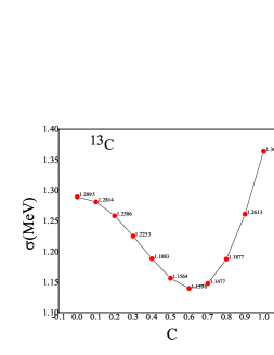
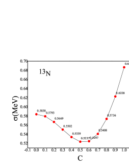
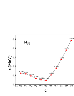
Figure 5: The root mean square deviation as a function of the control parameter C for three-cluster nuclei.

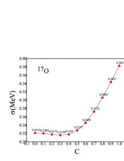
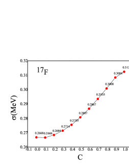
Figure 6: The root mean square deviation as a function of the control parameter C for four-cluster nuclei.

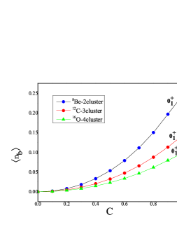
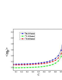
Figure 7: The expectation values of the vector-boson number operator for the lowest states as a function of control parameter C for N=10.

References

- (1) Iachello, F., Iachello, F., Arima, A., and Iachello, F. (1987). The interacting boson model. Cambridge University Press.
- (2) Iachello, F., and Levine, R. D. (1995). Algebraic theory of molecules. Oxford University Press.
- (3) Bijker, R. (2012). Spectrum generating algebras for few-body systems. In Journal of Physics: Conference Series (Vol. 380, No. 1, p. 012003). IOP Publishing.
- (4) Bijker, R., and Iachello, F. (2017). The algebraic cluster model: Structure of . Nuclear Physics A, 957, 154-176.
- (5) Bijker, R., and Iachello, F. (2000). Cluster states in nuclei as representations of a group. Physical Review C, 61(6), 067305.
- (6) Bijker, R., and Iachello, F. (2002). The algebraic cluster model: Three-body clusters. Annals of Physics, 298(2), 334-360.
- (7) Iachello, F., and Jackson, A. D. (1982). A phenomenological approch to -clustering in heavy nuclei. Physics Letters B, 108(3), 151-154.
- (8) Iachello, F. (1983). Algebraic approach to nuclear structure. Nuclear Physics A, 396, 233-243.
- (9) Daley, H., and Iachello, F. (1983). Alpha-clustering in heavy nuclei. Physics Letters B, 131(4-6), 281-284.
- (10) Iachello, F., Mukhopadhyay, N. C., and Zhang, L. (1991). Spectrum-generating algebra for stringlike mesons: Mass formula for mesons. Physical Review D, 44(3), 898.
- (11) Iachello, F., and Kusnezov, D. (1992). Radiative decays of mesons. Physical Review D, 45(11), 4156.
- (12) Bijker, R., Iachello, F., and Leviatan, A. (1994). Algebraic models of hadron structure. I. Nonstrange baryons. Annals of Physics, 236(1), 69-116.
- (13) Bijker, R., Iachello, F., and Leviatan, A. (2000). Algebraic models of hadron structure: II. Strange baryons. Annals of Physics, 284(1), 89-133.
- (14) Bijker, R., Dieperink, A. E. L., and Leviatan, A. (1995). Spectrum-generating algebra for molecules. Physical Review A, 52(4), 2786.
- (15) Bijker, R., and Leviatan, A. (1998). Algebraic treatment of three-body problems. Few-Body Systems, 25(1-3), 89-10
- (16) Bijker, R., and Iachello, F. (2014). Evidence for Tetrahedral Symmetry in . Physical review letters, 112(15), 152501.
- (17) Majarshin, A. J., Sabri, H., Jafarizadeh, M. A. and Amiri, N. (2018). Energy spectra of vibron and cluster models in molecular and nuclear systems. The European Physical Journal A, 54(3), 36.
- (18) von Oertzen, W., Freer, M., and Kanada-En’yo, Y. (2006). Nuclear clusters and nuclear molecules. Physics Reports, 432(2), 43-113.
- (19) Hiura, J., and Shimodaya, I. (1963). Alpha-Particle Model for . Progress of Theoretical Physics, 30(5), 585-600.
- (20) Abe, Y., Hiura, J., and Tanaka, H. (1973). A molecular-orbital model of the atomic nuclei. Progress of Theoretical Physics, 49(3), 800-824.
- (21) Okabe, S., Abe, Y., and Tanaka, H. (1977). The Structure of Nucleus by a Molecular Model. I. Progress of Theoretical Physics, 57(3), 866-881.
- (22) Okabe, S., and Abe, Y. (1979). The Structure of by a Molecular Model. II. Progress of Theoretical Physics, 61(4), 1049-1064.
- (23) Feldmeier, H., and Schnack, J. (2000). Molecular dynamics for fermions. Reviews of Modern Physics, 72(3), 655.
- (24) Roth, R., Neff, T., Hergert, H., and Feldmeier, H. (2004). Nuclear structure based on correlated realistic nucleon–nucleon potentials. Nuclear Physics A, 745(1-2), 3-33.
- (25) Neff, T., and Feldmeier, H. (2003). Cluster structures within fermionic molecular dynamics. arXiv preprint nucl-th/0312130.
- (26) Neff, T., Feldmeier, H., and Roth, R. (2005). Structure of light nuclei in Fermionic Molecular Dynamics. Nuclear Physics A, 752, 321-324.
- (27) Kanada-En’yo, Y., and Horiuchi, H. (2001). Structure of light unstable nuclei studied with antisymmetrized molecular dynamics. Progress of Theoretical Physics Supplement, 142, 205-263.
- (28) Kanada-En’yo, Y., Kimura, M., and Horiuchi, H. (2003). Antisymmetrized Molecular Dynamics: a new insight into the structure of nuclei. Comptes Rendus Physique, 4(4-5), 497-520.
- (29) Kanada-En’yo, Y., and Horiuchi, H. (2003). Cluster structures of the ground and excited states of studied with antisymmetrized molecular dynamics. Physical Review C, 68(1), 014319.
- (30) Brink, D. M., Friedrich, H., Weiguny, A., and Wong, C. W. (1970). Investigation of the alpha-particle model for light nuclei. Physics Letters B, 33(2), 143-146.
- (31) Della Rocca, V., Bijker, R., and Iachello, F. (2017). Single-particle levels in cluster potentials. Nuclear Physics A, 966, 158-184.
- (32) Bijker, R., and Iachello, F. (2019). Evidence for Triangular Symmetry in . Physical review letters, 122(16), 162501.
- (33) Leviatan, A., and Kirson, M. W. (1988). Intrinsic and collective structure of an algebraic model of molecular rotation-vibration spectra. Annals of Physics, 188(1), 142-185.
- (34) Roosmalen, O. S. V. (1982). Algebraic descriptions of nuclear and molecular rotation-vibration spectra (Doctoral dissertation, Rijksuniversiteit Groningen).
- (35) Iachello, F., and Levine, R. D. (1982). Algebraic approach to molecular rotation‐vibration spectra. I. Diatomic molecules. The Journal of Chemical Physics, 77(6), 3046-3055.
- (36) Bijker, R. (2010, December). Algebraic cluster model with tetrahedral symmetry. In AIP Conference Proceedings (Vol. 1323, No. 1, pp. 28-39). AIP.
- (37) Kramer, P., and Moshinsky, M. (1966). Group theory of harmonic oscillators (III). States with permutational symmetry. Nuclear Physics, 82(2), 241-274.
- (38) Pan, F., and Draayer, J. P. (1998). New algebraic solutions for transitional nuclei in the interacting boson model. Nuclear Physics A, 636(2), 156-168.
- (39) Pan, F., Zhang, X., and Draayer, J. P. (2002). Algebraic solutions of an sl-boson system in the transitional region. Journal of Physics A: Mathematical and General, 35(33), 7173.
- (40) Iachello, F., and Arima, A. (1974). Boson symmetries in vibrational nuclei. Physics Letters B, 53(4), 309-312.
- (41) Tilley, D. R., Kelley, J. H., Godwin, J. L., Millener, D. J., Purcell, J. E., Sheu, C. G., and Weller, H. R. (2004). Energy levels of light nuclei A= 8, 9, 10. Nuclear Physics A, 745(3-4), 155-362.
- (42) Ajzenberg-Selove, F. (1979). Energy levels of light nuclei . Nuclear Physics A, 320(1), 1-224.
- (43) Ajzenberg-Selove, F. (1984). Energy levels of light nuclei . Nuclear Physics A, 413(1), 1-168.
- (44) Jolie, J., Cejnar, P., Casten, R. F., Heinze, S., Linnemann, A., and Werner, V. (2002). Triple point of nuclear deformations. Physical review letters, 89(18), 182502.
- (45) Pan, F., Zhang, Y., and Draayer, J. P. (2005). Quantum phase transitions in the large-N limit. Journal of Physics G: Nuclear and Particle Physics, 31(9), 1039.
- (46) Zhang, Y., Hou, Z. F., and Liu, Y. X. (2007). Distinguishing a first order from a second order nuclear shape phase transition in the interacting boson model. Physical Review C, 76(1), 011305.
- (47) Zhang, Y., Hou, Z. F., Chen, H., Wei, H., and Liu, Y. X. (2008). Quantum phase transition in the vibron model and the symmetry. Physical Review C, 78(2), 024314.