Efficient comparison of independence structures of log-linear models

Abstract

Log-linear models are a family of probability distributions which capture relationships between variables. They have been proven useful in a wide variety of fields such as epidemiology, economics and sociology. The interest in using these models is that they are able to capture context-specific independencies, relationships that provide richer structure to the model. Many approaches exist for automatic learning of the independence structure of log-linear models from data. The methods for evaluating these approaches, however, are limited, and are mostly based on indirect measures of the complete density of the probability distribution. Such computation requires additional learning of the numerical parameters of the distribution, which introduces distortions when used for comparing structures. This work addresses this issue by presenting the first measure for the direct and efficient comparison of independence structures of log-linear models. Our method relies only on the independence structure of the models, which is useful when the interest lies in obtaining knowledge from said structure, or when comparing the performance of structure learning algorithms, among other possible uses. We present proof that the measure is a metric, and a method for its computation that is efficient in the number of variables of the domain.

[1]organization=Laboratorio de Investigación en Cómputo Paralelo/Distribuido (LICPaD) – Universidad Tecnológica Nacional, Facultad Regional Mendoza, addressline=Rodríguez 273, postcode=CP 5500,city=Ciudad de Mendoza, Mendoza, country=Argentina

[2]organization=Consejo Nacional de Investigaciones Científicas y Técnicas (CONICET), addressline=Av. Ruiz Leal s/n Parque General San Martín, postcode=CP 5500, city=Ciudad de Mendoza, Mendoza, country=Argentina

[3]organization=Laboratorio DHARMa – Universidad Tecnológica Nacional, Facultad Regional Mendoza, addressline=Rodríguez 273, postcode=CP 5500,city=Ciudad de Mendoza, Mendoza, country=Argentina

1 Introduction and Motivation

This paper presents a metric for efficiently comparing the independence structures of two log-linear models, a well-known representation of probability distributions over the assignments of discrete domains [1, 2, 3, 4, 5]. These models are widely used for representing real-world distributions in many different disciplines, such as epidemiology [6, 7, 8], economics [Lundtofte and Wilhelmsson [2013], ] and sociology [Raftery_2001, Schwartz_2016, Bucca_2019]. Due to the complexity of data analysis and the rapidly growing availability of large quantities of data, interest in the automatic learning of these models from data has increased, becoming a subfield of machine learning [DELLAPIETRA97, MCCALLUM03, LeealNIPS06, davis2010bottom, lowd14a, van2012markov]. In this area, the problem of automatically learning a structure from data is often divided into structure learning and parameter learning. The former involves finding a set of dependencies that best represent the relationships among the variables in the domain, while the latter consists in estimating the parameters that quantify the structure. The contribution of this work is inspired by the structure learning problem, which, in general, has two main objectives. Structures are either used as an intermediate step toward the construction of complete density models for inference tasks, such as the estimation of marginal and conditional probabilities (which is known as density estimation) [lowd14a, van2012markov, davis2010bottom]; or they are used as an interpretable model that shows the most significant interactions of a domain (known as knowledge discovery) [LeealNIPS06, haaren2013, claeskens2015, nyman2014context, pensar2017marginal]. To date, there are no direct methods for the evaluation of the quality of structures of log-linear models, despite their importance for obtaining accurate predictions and, perhaps more importantly, their crucial role when trying to understand patterns present in data and to draw reliable conclusions from those patterns. Our proposal offers a metric that can be used for several purposes, including the assessment of learning algorithms, knowledge discovery, and the design of new algorithms. To the best of our knowledge, our proposal is the first of its kind, with no other structural distance metric in the literature for evaluating log-linear models in terms of their context-specific independencies.

In this work we make references to and draw inspiration from Markov networks, an interesting subset of the family of log-linear models, whose independence structure is an undirected graph, with the nodes representing the random variables of the domain, and the edges encoding direct probabilistic influence between the variables. There are several methods for learning Markov network structures from data [brombergmargaritis09b, schluter2014ibmap, pensar2017marginal, schluter2018blankets]. In undirected graphical models (UGMs), the absence of an edge indicates that the dependence could be mediated by some other subset of variables, corresponding to conditional independence between these variables. The use of graphs as representation, however, has an important disadvantage: since it simply uses the basic concept of conditional and marginal independence, this representation may hide the occurrence of fine-grain structure such as context-specific independencies [boutilier1996context, hojsgaard2004statistical, 4], which are independencies that hold only in a subspace of the configurations of the conditioning set. Log-linear models are more flexible than graphical models, since they are capable of encoding not only conditional independencies, but also context-specific independencies. The log-linear representation of the structure is defined as a set of feature functions, each consisting of an assignment to some subset of the variables in the domain. Given a set of features, the joint probability distribution is completely specified by the feature weights, one real number per feature, which are the numerical parameters of the log-linear model.

For the structure learning problem, there has been a surge of interest towards methods that construct a log-linear model by selecting features from a dataset, usually by performing a local search that incrementally adds or deletes features [DELLAPIETRA97, LeealNIPS06, davis2010bottom, van2012markov, lowd2013learning, lowd14a]. This approach defines structure learning as a feature selection problem, where the features represent dependencies between subsets of random variables. All these contributions have only been assessed for the density estimation goal of learning, that is, the selection of models for inference tasks, by measuring the quality of learned models in terms of prediction performance. The reason for this is that, historically, this family of models has rarely been used with the goal of knowledge discovery in mind, given that the interpretability of conventional log-linear models is burdensome, and reading independencies from them is not trivial. However, this has been changing lately, mainly due to the fact that the theory of log-linear models for contingency tables [darroch1980markov] has been augmented by the introduction of a variety of representations that generalize graph-based undirected graphical models: Context-Specific Interaction models [eriksen1999context, hojsgaard2004statistical], Stratified-graphical models [nyman2014stratified, nyman2014context], and Canonical models [ederaSchluterBromberg14]. Such contributions have shifted attention towards methods that focus on learning only the structure of these models, while the parameter learning step may be performed afterwards with existing techniques, or not performed at all, depending on the use case. Although the focus of this work is on log-linear models for categorical data, it is interesting to mention other models that are able to represent context-specific interactions, for example, in domains based on ordinal data, such as Hierarchical Marginal Models [nicolussiContextspecificIndependenciesHierarchical2019]; or causal models, such as CPT-tress [boutilier1996context] and Labeled Directed Acyclic Graphs (LDAGs) [PENSAR201691, coranderLogicalApproachContextspecific2019]. In these representations, the semantics for reading conditional independence from graphs serves as inspiration for graphically expressing context-specific independencies, with the aim of representing a much wider class of models while maintaining their interpretability.

Due to all these relatively recent developments that focus on the structures of the models, there is an incresing need for tools that assess the quality of structure learning methods. At present, this assessment is often carried out with the Kullback–Leibler divergence (KL-divergence) [kullback1951information, cover2012elements]. In this context, the KL-divergence measures the similarity of the complete distributions encoded by each structure together with their parameters [ederaSchluterBromberg14, edera2014grow]. Initially, divergences were the only means of computing statistical distance. For model comparisons they have been used mainly in the process of disproving the null-hypothesis, in which one model differs from the other when the divergence equals zero. However, they present some limitations when the null-hypothesis holds, i.e., when the models are different, as they provide no sense of scale for their difference. In that case, the statistical community uses distance functions or measures[DODGE2006], a.k.a. metrics, a notion stronger than divergence that satisfies not only nonnegativity and discrimination, but also symmetry and the triangle inequality. Since the KL-divergence is a measure of divergence between distributions, it is an indirect procedure that requires learning the parameters in addition to the structure; therefore, the quality of structures is analyzed by evaluating the quality of the resulting full distribution. This introduces some shortcomings. The first disadvantage is that false positives and false negatives have a different impact on the quality of the distribution. False negatives cannot be mitigated by the numerical parameters, because they add incorrect independence assumptions to the distribution that can invalidate statistical inference, leading to faulty conclusions. Instead, false positives may be mitigated when learning the parameters, by setting some weights to zero to encode the independencies that were not found by structure learning. Thus, KL is unable to accurately measure false positives in the structure, since these can be obscured by the parameters. As a second disadvantage, it is important to note that the parameter learning process is sensitive to data scarceness; therefore, the KL measure might not be accurate when data is insufficient. Both shortcomings are illustrated by a toy example in Section 7. Since our method is computed directly over the structures, it addresses both problems: it allows for a separate analysis of false positives and false negatives, and is not influenced by data scarceness.

When learning structures for high-dimensional domains, the computation of the KL-divergence becomes infeasible and some works report instead the Conditional Marginal Log-likelihood (CMLL) [LeealNIPS06, davis2010bottom, van2012markov, lowd2013learning, lowd14a], which uses marginal probabilities in order to avoid the computation of the partition function that normalizes the distribution. Although useful in practice, CMLL is an approximate method, and it also presents the first and second shortcomings mentioned above, because it also requires the task of learning the numerical parameters of the structure. Lastly, as a means of understanding structural qualities without taking into account the parameters, a few works have used the number of features and average feature length [van2012markov, ederaSchluterBromberg14, edera2014grow]. Both are aggregated and indirect indicators and as such not very informative; moreover, they do not allow for trustworthy comparison between different structures. A summary of the characteristics of all these methods is provided in Table 1.

Measure	Advantages	Disadvantages
KL-divergence	•   ease of implementation • satisfies nonnegativity and discrimination	•   not a metric (symmetry, triangle inequality) • unable to measure FPs in the structure • sensitive to data scarceness • infeasible in high dimensions
CMLL	•   scalability	•   unable to measure FPs in the structure • sensitive to data scarceness • uses an approximation
Number of features	•   parameter-independent • correlates to # of dependencies	•   indirect measure
Average feature length	•   parameter-independent • provides an idea of the density of the structure	•   indirect measure

Table 1: Characteristics of measures for the comparison of log-linear models

Our method works by measuring the number of structural differences that appear between two log-linear models, efficiently producing a confusion matrix that counts the true positives, false positives, true negatives and false negatives that appear in the second model, relative to the first one. It is inspired on the structure comparison method of Markov networks: the Hamming distance of their graphs [brombergmargaritis09b, schluter2014ibmap, pensar2017marginal, schluter2018blankets], i.e., the sum of false positives plus false negatives in terms of edges. Although there is no unequivocal graph representation for log-linear models and therefore no straightforward generalization of the Hamming distance for this case, we will show that both measures take advantage of different properties of their respective independence representations in order to reduce the complexity of the comparison. As will be discussed in detail later in Section 3, a straightforward counting of dependencies and independencies for producing the confusion matrix for log-linear models presents an exponential computational cost due to the much larger space of possible structures when compared to graphical models. The main advantage of our method is that it can efficiently compute the counts in the confusion matrix with respect to the number of variables. Nevertheless, the efficiency w.r.t. the number of features is not guaranteed for a large number of features in the models, and it will be the subject of future work.

The contribution of this work has several potential applications. Most notably, this technique can be used to improve the quality of structures learned from data by providing the means for comparing different structure learning techniques over synthetic data produced by a known underlying distribution. This is achieved by comparing the quality of the structures obtained from data by any given algorithm, measured as the distance from the learned structure to the structure of the underlying distribution. Better structures have important advantages as they can improve both the quality and efficiency of parameter learning, leading to better density models for inference tasks. In addition, although the complexity of the structures of log-linear models has been a limiting factor in the past, recent contributions have allowed for knowledge discovery tasks, by improving the interpretability of the models with some of the representations mentioned above. Therefore, our method can also contribute to this goal, by providing a tool that can help select among different algorithms, or algorithm configurations, in order to find the best learning strategies specifically based on the quality of structures, which is not achievable with the state-of-the-art methods. While these are the main benefits we identify for our contribution, there might be many other potential use cases. For instance, another aspect of experimentation that could be explored is the possibility of generating random synthetic structures from the space of possible structures, using their structural distance as a guarantee that the sample is not biased. At present, these synthetic experiments are usually comprised of a small number of handmade structures, designed in order to highlight the advantages of a particular method. In addition, we see an interesting possibility of application in the incorporation of this measure as a means of assessing similarities among structures in search algorithms, where each solution in the search space would be equivalent to a complete log-linear model structure. A similar example in the space of features is in [davis2010bottom], where a measure of similarity among features is used to generate the nearest candidate features w.r.t. a given feature from the current structure, in order to guide the search. Lastly, another use case can be found in the design of new log-linear structure learning algorithms. If an algorithm poses the structure learning problem as a search in the space of possible structures (feature sets), then our metric could be used in different ways to evaluate similarity between structures, e.g. to find similar structures in a proximity search, or to maintain diversity by encouraging the generation of structures that differ from each other. Lastly, it should be noted that our method is efficient in two ways: on the one hand, it is proven to be efficient in the number of variables of the models, when compared to a brute force approach; on the other hand, it avoids the complexity of parameter learning when used as a substitute for methods that compare the complete distributions.

This paper is organized as follows: In the next section we present the notation and main concepts required for our analysis. Section 3 establishes and justifies the basis for our approach, by introducing a brute-force method for the structural comparison of log-linear models, highlighting its sources of exponentiality, and providing a roadmap for tackling them. Section 4 presents our approach for the efficient computation of the confusion matrix, together with a proof of correctness. Section 5 introduces a distance measure directly computable from the confusion matrix, and provides proof it is indeed a distance metric by proving all four properties: nonnegativity, discrimination, symmetry, and triangle inequality. Section 6 summarizes the main steps for the development of our contribution and for its computation. Section 7 describes the example comparison of our metric against KL-divergence, the most common measure used in recent works concerning log-linear models structure learning. Section 8 presents some conclusions, open questions and some ideas to extend this work. To simplify the presentation, the proofs of some lemmas have been removed from the main text and are presented in detail in B. Similarly, all auxiliary lemmas are described and proven in C.

2 Background knowledge and Notation

This section introduces key concepts of probabilistic models and the notation used to denote them throughout the manuscript. The first two parts, Sections 2.1 and 2.2, present basic definitions concerning random variables and log-linear models, together with some notations specific to this work. The remaining three sections are more involved and present crucial aspects of our contribution. Firstly, in Section 2.3, we define different kinds of probabilistic independencies and reproduce important equivalences. Secondly, Section 2.4 explains the structure representation on which our contribution is conceptually based. Finally, Section 2.5 provides an overview of an analogous strategy used for the comparison of Undirected Graphical Models (UGMs), that serves as a partial inspiration for our method.

2.1 Random Variables

Let V be a finite set of indices for a set of discrete random variables $X_{V}$. Lowercase subscripts denote single indices (e.g., $X_{i},X_{j}\in X_{V}$ where $i,j\in V$), while uppercase subscripts denote subsets of indices (e.g., $X_{A}\subseteq X_{V}$ where $A\subseteq V$). A variable $X_{k}$ can take a value from a finite set of configurations, denoted by $val(X_{k})$. For example, for a binary variable $X_{0}$, $val(X_{0})=\{0,1\}$. An arbitrary configuration in $val(X_{k})$ will be denoted in lowercase, e.g., $x_{k}$.

A set of variables $X_{A}$, $A\subseteq V$, can take values from the cross-product of $val(X_{k})$, over all $k\in A$; with individual configurations denoted by $x_{A}$. The set of variables assigned in some configuration $x$ is called the scope of $x$, denoted $S_{x}$; e.g., for $x=x_{A}$, $S_{x}=X_{A}$.

The space of all configurations for $X_{V}$ is denoted as $\mathcal{X}$. A canonical context $x$ is a complete assignment in a domain, i.e., $x\in\mathcal{X}$, and $S_{x}=X_{V}$. Even though canonical contexts are not used in this work in this manner, we make extensive use of a similar concept: fully-contextualized (FC) contexts (or simply contexts when the meaning is clear), which are configurations defined for a given pair of indices $(i,j)$ and consist of assignments to all variables in $X_{V}\setminus\{X_{i},X_{j}\}$. The set of all FC contexts for one $(i,j)$ is denoted as $\mathcal{X}^{ij}$. Its name stems from the fact that it is used in the sense of a completely contextualized conditioning set.

2.2 Log-linear models

For a distribution to be considered an element of the log-linear family it must be structured through a set of feature functions $F=\{f_{i}(X_{D_{i}})\}$, and specify a numerical value $\theta_{i}$ for each assignment $x_{D_{i}}$ of the subset of variables $X_{D_{i}}$, where $D_{i}\subseteq V$, resulting in the following generic functional form of distributions in the log-linear family:

$$p(x)=\frac{1}{Z(\theta)}\,exp\left(\sum_{f_{i}\in F}\theta_{i}f_{i}(x_{D_{i}})\right),$$ (1)

where $Z(\theta)$ is the partition function that ensures that the distribution is normalized (i.e., all entries sum to $1$).

In what follows, features are denoted by lowercase letters, such as $f$, $g$ or $h$. The value that variable $X_{k}\in X_{V}$ takes in feature $f$ is denoted by $X_{k}(f)$. For example, if $f=<X_{0}=1,X_{2}=0,X_{3}=1>$, then $X_{2}(f)=0$. Also, overloading the naming used for variable configurations, the set of variables that are assigned in a feature $f$ is called the $scope$ of $f$, and it is denoted by $S_{f}$. For the last example, $S_{f}=\{X_{0},X_{2},X_{3}\}$.

Finally, we introduce the notation ${h}^{ij}$ to denote a feature composed of the same assignments as feature $h$, except for those of $X_{i}$ and $X_{j}$, when $i,j$ is a pair of distinct indices such that $X_{i},X_{j}\in S_{h}$. For instance, if $V=\{0,\dots,5\}$, and if

$$h=<X_{0}=2,X_{1}=1,X_{2}=1,X_{5}=0>,$$

then the same feature without the pair of assignments to $(X_{0},X_{2})$ will be

$$h^{02}=<X_{1}=1,X_{5}=0>.$$

2.3 Independence

We use the notation $(X_{A}\mbox{$\perp\!\!\!\!\perp$}X_{B}\mid X_{C})_{p}$ to denote that in the distribution $p$, variables in set $X_{A}$ are (jointly) independent of those in $X_{B}$, conditioned on the values of the variables in $X_{C}$, for disjoint sets of indices $A$, $B$, and $C$. This occurs if and only if the conditional distribution of $X_{A}$ conditioned on the values of variable $X_{B}$ and $X_{C}$ only depends on the values of $X_{C}$. Formally,

$$(X_{A}\mbox{$\perp\!\!\!\!\perp$}X_{B}\mid X_{C})_{p}\iff p(x_{A}|x_{B},x_{C})=p(x_{A}|x_{C}),$$

for all $x_{A}\in val(X_{A})$, $x_{B}\in val(X_{B})$ and $x_{C}\in val(X_{C})$. The negation is $(X_{A}\mbox{$\perp\!\!\!\!\perp\!\!\!\!\!\not~{}~{}~{}$}X_{B}\mid X_{C})_{p}$, which denotes conditional dependence. $I({X_{A}},{X_{B}}\mid X_{C})_{p}$ denotes a query of conditional independence, i.e., a question of whether the independence $(X_{A}\mbox{$\perp\!\!\!\!\perp$}X_{B}\mid X_{C})$ holds or not; symbolically:

$$I({X_{A}},{X_{B}}\mid X_{C})_{p}\text{ is true }\iff(X_{A}\mbox{$\perp\!\!\!\!\perp$}X_{B}\mid X_{C})_{p}.$$

A context-specific independence [boutilier1996context, hojsgaard2004statistical, 4] between variables $X_{A}$ and $X_{B}$ given variables $X_{C}$ and a set of configurations (context) $X_{D}=x_{D}$, where $D\cap A\cap B\cap C=\emptyset$, is defined as

$$(X_{A}\mbox{$\perp\!\!\!\!\perp$}X_{B}\mid X_{C},x_{D})_{p}\iff p(x_{A}|x_{B},x_{C},x_{D})=p(x_{A}|x_{C},x_{D}),$$

for all assignments $x_{A}\in val(X_{A})$, $x_{B}\in val(X_{B})$ and $x_{C}\in val(X_{C})$, whenever $p(X_{B},X_{C},x_{D})>0$. A context-specific dependence is denoted by $(X_{A}\mbox{$\perp\!\!\!\!\perp\!\!\!\!\!\not~{}~{}~{}$}X_{B}\mid X_{C},x_{D})_{p}$; and $I({X_{A}},{X_{B}}\mid X_{C},x_{D})_{p}$ is a context-specific independence query.

From the above, it is easy to prove the following equivalence of context-specific independencies:

$$(X_{i}\mbox{$\perp\!\!\!\!\perp$}X_{j}\mid x_{U},X_{W})\equiv\forall x_{W}\in val(X_{W}),(X_{i}\mbox{$\perp\!\!\!\!\perp$}X_{j}\mid x_{U},x_{W}),$$ (2)

or, equivalently,

$$(X_{i}\mbox{$\perp\!\!\!\!\perp\!\!\!\!\!\not~{}~{}~{}$}X_{j}\mid x_{U},X_{W})\equiv\exists x_{W}\in val(X_{W}),(X_{i}\mbox{$\perp\!\!\!\!\perp\!\!\!\!\!\not~{}~{}~{}$}X_{j}\mid x_{U},x_{W}),$$ (3)

for all $X_{i}\neq X_{j},\,U\cap W=\emptyset,\,U\cup W\subseteq{V}\setminus\{i,j\},\,x_{U}\in val(X_{U})$.

One key result of probabilistic models consists of the separation of the independence semantics of the distribution into an explicit structure. Interestingly, for log-linear distributions, this structure is completely encoded by its set of features $F$. In other words, the set of features $F$ is sufficient for determining dependence or independence, which is formalized by replacing $p$ as the subscript in the notation of independencies, e.g., $(X_{A}\mbox{$\perp\!\!\!\!\perp$}X_{B}\mid X_{C},x_{D})_{F}$, and dependencies, e.g., $(X_{A}\mbox{$\perp\!\!\!\!\perp$}X_{B}\mid X_{C},x_{D})_{F}$.

We shall start with some intuitions, to then proceed with the formalization of these concepts. For that, we first note that the numerical parameters $\theta_{i}$ in the logarithmic representation of Eq. 1 can take any real value. Non-null terms, i.e., $\theta_{i}\neq 0$, indicate the presence of probabilistic interactions among the variables that appear together in the scope of a feature. In contrast, when $\theta_{i}=0$ for some $i$, the corresponding feature ’’disappears” from the model and, as a consequence, the interactions between the variables in its scope also vanish. Thus, the notion of independence is related to setting certain parameters to $0$. The set of all features $F$ in a log-linear model, allows for any marginal, conditional or context-specific independence query to be verified.

First, we will formalize this idea for the (strictly) context-specific case, and show how the other types of (in)dependencies can be deduced from it.

Given a context $x_{U}$, a (strictly) context-specific independence of the form $(X_{i}\mbox{$\perp\!\!\!\!\perp$}X_{j}\mid x_{U})_{F}$ is verified, firstly, by considering all features in $F$ that are ’’compatible‘‘ with $x_{U}$, i.e.,

$$F^{\prime}=\left\{f\in F\,\middle|\,\forall u\in U,X_{u}\in S_{f}\implies X_{u}(x_{U})=X_{u}(f)\right\};$$ (4)

that is, for every variable $X_{u}$ in the context $x_{U}$ that is also in the context of $f$ (represented by $S_{f}$), it is the case that their assigned values in the context $x_{U}$ and in feature $f$ are equal.

Secondly, for the independence to hold, it must be verified that no feature in $F^{\prime}$ contains both $X_{i}$ and $X_{j}$ in its scope:

$$(X_{i}\mbox{$\perp\!\!\!\!\perp$}X_{j}\mid x_{U})_{F}\iff\forall f\in F^{\prime},\,X_{i}\not\in S_{f}\vee X_{j}\not\in S_{f}.$$ (5)

In order to read the most general context-specific independencies of the form $(X_{i}\mbox{$\perp\!\!\!\!\perp$}X_{j}\mid x_{U},X_{W})_{F}$, the following equivalence [hojsgaard2004statistical, ederaSchluterBromberg14, PENSAR201691] can be used:

$$(X_{i}\mbox{$\perp\!\!\!\!\perp$}X_{j}\mid X_{U\cup W})_{F}\equiv\forall x_{U}\in val(X_{U}),\,(X_{i}\mbox{$\perp\!\!\!\!\perp$}X_{j}\mid x_{U},X_{W})_{F}.$$ (6)

From the feature set representation, we begin by verifying a set of independencies where the whole conditioning set is contextualized ($X_{W}=\emptyset$) and can later aggregate any subset of variables in $U$ for which the equivalence in Eq. 6 holds, which allows us to obtain the truth value for the most general type of queries $(X_{i}\mbox{$\perp\!\!\!\!\perp$}X_{j}\mid x_{U},X_{W})_{F}$, which also includes all queries where $x_{U}=\emptyset$ (conditional independencies). Therefore, any conditional (in)dependence can be read from the set of features of a log-linear model. Lastly, marginal independencies $(X_{i}\mbox{$\perp\!\!\!\!\perp$}X_{j})$ are simply conditional independencies among $X_{i}$ and $X_{j}$ that hold for all conditioning sets, and can thus be deduced by verifying a set of conditional independencies.

2.4 Dependency models

Given the set of features $F$, it is then straightforward to read (in)dependencies of any given pair of variables conditioned on any partially contextualized conditioning set. Alternatively, [PEARL88] proposes an explicit representation of the (in)dependencies of the distribution: the dependency model, an exhaustive listing of all dependencies in the distribution. For the case of the well-known undirected graphical models (UGMs), for instance, the dependency model reports, for each pair of variables, whether they are dependent given each possible conditioning set of variables. To formalize it, it is convenient to first define the set of all possible triplets of variable pairs and conditioning set for some given set $V$ of random variables,

$$\mathcal{T}^{UGM}=\left\{\ I({X_{i}},{X_{j}}\mid X_{U})\ \ \middle|\ \begin{array}[]{ll}i\neq j\in V,\\ U\subseteq V\setminus\{i,j\}\end{array}\right\},$$ (7)

to then define the dependency model of some undirected model $H$ as

$$\mathcal{D}^{UGM}_{C}(H)=\left\{\ I({X_{i}},{X_{j}}\mid X_{U})\in\mathcal{T}^{UGM}\ \ \middle|\ (X_{i}\mbox{$\perp\!\!\!\!\perp\!\!\!\!\!\not~{}~{}~{}$}X_{j}\mid X_{U})_{H}\ \right\}.$$ (8)

We use the superscript $UGM$ to clarify that this set can encode the (in)dependencies of UGMs, which excludes context-specific structure. The subscript $C$ (for ’’complete”) is used as part of our notation of the dependency model to contrast the exhaustive definitions from an approximate version defined in the following section.

Log-linear distributions are more complex in that they can encode not only marginal and conditional dependencies, but also context-specific dependence assertions. This requires a generalization from the idea of a dependency model to a context-specific dependency model. As for the undirected case, we formalize it in two steps, starting by the set of contextualized triplets:

$$\mathcal{T}=\left\{\ I({X_{i}},{X_{j}}\mid x_{U},X_{W})\ \ \middle|\ \ \begin{array}[]{ll}i\neq j\in V;\\ U,W\subseteq V\setminus\{i,j\};\\ U\cap W=\emptyset;\\ x_{U}\in val(X_{U})\end{array}\right\},$$

to then define the context-specific dependency model (of a log-linear structure $F$) as

$$\mathcal{D}_{C}(F)=\left\{\ I({X_{i}},{X_{j}}\mid x_{U},X_{W})\in\mathcal{T}\ \ \middle|\ \ (X_{i}\mbox{$\perp\!\!\!\!\perp\!\!\!\!\!\not~{}~{}~{}$}X_{j}\mid x_{U},X_{W})_{F}\ \right\}.$$ (9)

where, again, the subscript $C$ denotes the completeness of this model, in contrast to its approximate version defined in Section 2.5.

Given that these dependency models are exhaustive, it is straightforward to determine the (in)dependence in model $F$ of any given assertion $t=I({X_{i}},{X_{j}}\mid x_{U},X_{W})$ by a simple verification of inclusion in a set; in this way, $t\in\mathcal{D}_{C}(F)$ indicates dependence $(X_{i}\mbox{$\perp\!\!\!\!\perp\!\!\!\!\!\not~{}~{}~{}$}X_{j}\mid x_{U},X_{W})_{F}$ is true for model $F$, while $t\notin\mathcal{D}_{C}(F)$ indicates that the independence $(X_{i}\mbox{$\perp\!\!\!\!\perp$}X_{j}\mid x_{U},X_{W})_{F}$ holds in that model.

2.5 Comparison of undirected graphical models

In the following section, we will show that log-linear models present several exponential complexities in their structure, the first of which is analogous to an exponentiality present in the space of structures of UGMs. Because of this, it may be helpful for the reader to understand such exponentiality in the case of UGMs and how it is overcome by the most widely used measure for comparing these models. In what follows, we provide a brief explanation of this common approach and its advantages. The underlying idea is that, by taking advantage of the properties of UGMs, their structures can be compared correctly and completely, avoiding an exhaustive comparison. These ideas have inspired one aspect of our own approximation, by using similar concepts that apply to the much larger class of log-linear models, and also our proof in Section 5, in which we used more general properties and equivalences that apply to the structures of log-linear models to obtain guarantees that this class of models are correctly and completely compared by our method.

As it can be seen in Eqs. 7 and  8, UGMs suffer from an exponentiality in the number of subsets $U\subseteq V\setminus\{i,j\}$. The approach for undirected graphical models compares them over the polynomial-size dependency model $\mathcal{D}^{UGM}$, a subset of $\mathcal{D}^{UGM}_{C}$ containing only fully conditional dependencies defined as the dependencies in $\mathcal{D}^{UGM}_{C}$ with a maximum-size conditioning set $U$, i.e., $U=V\setminus\{i,j\}$. Formally,

$$\mathcal{D}^{UGM}(H)\equiv\left\{\ I({X_{i}},{X_{j}}\mid X_{U})\in\mathcal{T}^{UGM}\ \ \middle|\ (X_{i}\mbox{$\perp\!\!\!\!\perp\!\!\!\!\!\not~{}~{}~{}$}X_{j}\mid X_{U})_{H},\,\,\,U=V\setminus\{i,j\}\ \right\}.$$

The comparison based on fully conditional dependencies corresponds to the known approach for the comparison of two undirected graphical models: the Hamming distance of their graphs, as according to the pairwise Markov property [PEARL88] this reduced set is nothing more than the edges of the undirected graph, i.e.,

$$(X_{i}\mbox{$\perp\!\!\!\!\perp\!\!\!\!\!\not~{}~{}~{}$}X_{j}\mid X_{V\setminus\{i,j\}})_{H}\equiv(X_{i},X_{j})\in E,$$

where $E$ is the set of edges of the graph representation of model $H$.

Despite only being conducted on the subset of the fully conditional dependencies, the Hamming distance comparison satisfies the properties of a metric: nonnegativity, symmetry, discrimination, and triangle inequality[DODGE2006, aliprantis2006]. The first guarantees that the measure is greater than zero for every possible input. The second property guarantees that the distance from one model to the other is the same as the distance from the second to the first. The third property guarantees that for any two undirected models $H_{1}$ and $H_{2}$, their distance is zero if and only if they are identical. And finally, the fourth property guarantees that given three models $H_{1}$, $H_{2}$ and $H_{3}$, the distance from $H_{1}$ to $H_{3}$ is always smaller than the sum of the distances between the other two, i.e., the distance from $H_{1}$ to $H_{2}$ plus the distance from $H_{2}$ to $H_{3}$.

For the Hamming distance of undirected graphs, the first two and the last properties are trivially satisfied. The second property is also easily verified on graphs; nevertheless, it is useful to also inquire whether the satisfaction of this property for graphs implies that the complete dependency models are also identical when the distance between graphs is zero. In other words, we would like to know if, when the reduced dependency models $\mathcal{D}^{UGM}(H_{1})$ and $\mathcal{D}^{UGM}(H_{2})$ are equal (Hamming distance of zero), then the complete dependency models $\mathcal{D}^{UGM}_{C}(H_{1})$ and $\mathcal{D}^{UGM}_{C}(H_{2})$ are also equal. To the best of our knowledge, this statement has no formal proof in the literature, yet we believe it is not difficult to prove. As an intuitive justification, let us note, first, that the equality over fully conditional dependencies is equivalent to the equality of the undirected graphs. By the Markov properties [5, 4], any (general) conditional dependence in $\mathcal{D}^{UGM}$ can be read from a graph, thus determining the complete model. Then, the equality of these subsets of dependencies implies the equality of the complete dependency models:

$$\mathcal{D}^{UGM}(H_{1})=\mathcal{D}^{UGM}(H_{2})\iff\mathcal{D}^{UGM}_{C}(H_{1})=\mathcal{D}^{UGM}_{C}(H_{2}).$$ (10)

3 Structure comparison between log-linear models

In this section we will show how to arrive at a formal definition of the sets in a confusion matrix for directly and thoroughly comparing the structures of log-linear models. The section begins by describing an exhaustive brute-force approach for this comparison, while highlighting its main sources of exponential computational complexities. Then, it motivates and formalizes some required approximations, and proves that, despite these approximations, the resulting comparison is valid. With this result, we can continue to address the remaining source of complexity in Section 4.

Comparing the structures of two log-linear models $F$ and $G$ implies comparing all the independencies and dependencies encoded in each of them. An exhaustive, straightforward approach for this comparison should examine each possible triplet from the set $\mathcal{T}$, testing its membership in both $\mathcal{D}_{C}(F)$ and $\mathcal{D}_{C}(G)$. Throughout this work we will use the convention that a positive case corresponds to a dependence or interaction, whereas the absence of an interaction is a negative case, in accordance with the comparison of UGMs. Then, the dependency model comparison results in a confusion matrix for $F$ and $G$, with two correct cases and two incorrect cases: if the triplet belongs to both, one count is added to true positives ($TP_{C}$); if the triplet is missing in both, it is counted as a true negative ($TN_{C}$); if $F$ does not contain the triplet but $G$ does, it is counted as a false positive ($FP_{C}$); and if the triplet belongs to $F$ but not to $G$, it counts as a false negative ($FN_{C}$). Formally,

$$TP_{C} =\left|\ \left\{\ t\in\mathcal{T}\mid t\in\mathcal{D}_{C}(F)\land t\in\mathcal{D}_{C}(G)\ \right\}\ \right|,$$ (11)

$$FN_{C} =\left|\ \left\{\ t\in\mathcal{T}\mid t\in\mathcal{D}_{C}(F)\land t\not\in\mathcal{D}_{C}(G)\ \right\}\ \right|,$$ (12)

$$FP_{C} =\left|\ \left\{\ t\in\mathcal{T}\mid t\not\in\mathcal{D}_{C}(F)\land t\in\mathcal{D}_{C}(G)\ \right\}\ \right|,$$ (13)

$$TN_{C} =\left|\ \left\{\ t\in\mathcal{T}\mid t\not\in\mathcal{D}_{C}(F)\land t\not\in\mathcal{D}_{C}(G)\ \right\}\ \right|,$$ (14)

where, again, the subscript $C$ denotes the fact that this confusion matrix is computed over the complete dependency models.

Unfortunately, the complexity of these evaluations depends directly on the cardinality of $\mathcal{T}$, which is exponential in three possible ways:

1. There is an exponential number of subsets of $V\setminus\{i,j\}$.

2. For each subset of $V\setminus\{i,j\}$, there is an exponential number of disjoint sets $U$ and $W$. In other words, let $S\subseteq V\setminus\{i,j\}$; then, for each possible $S$, we have that $U$ and $W$ can be all partitions of $S$ into two sets, plus the cases where $U=\emptyset,W=S$ and $U=S,W=\emptyset$.

3. For each possible $U$ and $W$ where $U$ is not empty, there is a number of contexts $x_{U}$ that is exponential in the size of $U$.

In order to give an intuition of the context-specific dependency model and its complexity, we provide a simple example.

Example 1.

Let $V=\{0,\dots,3\}$ be the index set of binary variables $X_{V}$. Any two log-linear models ${M}_{1}$ and ${M}_{2}$ over this domain can be represented by their context-specific dependency models $\mathcal{D}_{C}({M}_{1})$ and $\mathcal{D}_{C}({M}_{2})$, where each contains some subset of all possible marginal, conditional and context-specific dependency assertions, as summarized in Table 2.

Case	# of assertions	Examples
$U=W=\emptyset$	6	$I({X_{0}},{X_{2}})$
$|W|=1,U=\emptyset$	12	$I({X_{0}},{X_{1}}\mid X_{2})$
		$I({X_{0}},{X_{1}}\mid X_{3})$
$|W|=2,U=\emptyset$	6	$I({X_{0}},{X_{1}}\mid X_{2},X_{3})$
		$I({X_{1}},{X_{2}}\mid X_{0},X_{3})$
$W=\emptyset,|U|=1$	24	$I({X_{0}},{X_{1}}\mid X_{2}=0)$
		$I({X_{0}},{X_{1}}\mid X_{2}=1)$
$W=\emptyset,|U|=2$	24	$I({X_{0}},{X_{1}}\mid X_{2}=0,X_{3}=0)$
		$I({X_{0}},{X_{1}}\mid X_{2}=0,X_{3}=1)$
$|W|=1,|U|=1$	24	$I({X_{0}},{X_{1}}\mid X_{2}=0,X_{3})$
		$I({X_{0}},{X_{1}}\mid X_{2}=1,X_{3})$
		$I({X_{0}},{X_{1}}\mid X_{2},X_{3}=0)$

Table 2: Each row shows a subset of Eq. 9 for a domain with 4 binary variables. The first column determines the subset according to the cardinality of the conditioning sets, the second column indicates the number of assertions present in each subset, and the third column exemplifies a few of those assertions.

In total, with this representation, we would need to test 96 unique assertions per model in order to produce the counts of the confusion matrix (Eqs. 11 to 14) for ${M}_{1}$ and ${M}_{2}$.

Our proposal addresses the three exponentialities. The first one is addressed by adapting an approximation that is widely used for the subclass of UGMs, described in Section 2.5. Although the approach for these models is based on unassigned conditioning sets, it can be applied similarly to context-specific dependency models by considering only assertions in which $S=U\cup W=V\setminus\{i,j\}$. In this way, we reduce the number of possible sets $S$ from the power set of $V\setminus\{i,j\}$ to only one set per pair $(i,j)$.

Unfortunately, this has no impact on the second nor the third exponentialities, which are specific to this class of models. With the first reduction we have one choice of set $S$ per each pair of variables, but from each pair this set has an exponential number of assignments to $U$ and $W$; that is, there is an exponential number of ways of splitting the conditioning set into an assigned set and unassigned set. This second exponentiality is addressed through further reductions in the number of comparisons, by considering only assertions where $W=\emptyset$ and $U=V\setminus\{i,j\}$. The conditioning sets in these assertions thus correspond to $\mathcal{X}^{ij}$, the set of fully contextualized contexts as defined in Section 2.1. In what follows, we rename $U$ as $Z$ when referring to this case of fully-contextualized conditioning sets. This reduction is justified by the ability of context-specific structures to represent more general dependencies and independencies, based on the equivalences in Section 2.3 (in particular, Eq. 6 and its negation).

Both reductions are then formalized by defining $\mathcal{D}(F)$, a reduced version of the complete dependency model $\mathcal{D}_{C}(F)$ (for an arbitrary model $F$), that contains one assertion of the form $I({X_{i}},{X_{j}}\mid x_{Z})$ for every $X_{i}\neq X_{j}\in X_{V}$ and for every fully-contextualized context $x_{Z}\in\mathcal{X}^{ij}$. We define $\mathcal{D}(F)$ by formalizing the reduced set of triplets $\mathcal{T}_{FC}$ as

$$\mathcal{T}_{FC}=\left\{I({X_{i}},{X_{j}}\mid x_{Z})\ \ \middle|\ i\neq j\in V,\,\,\,x_{Z}\in\mathcal{X}^{ij}\right\},$$ (15)

to then define the reduced, fully-contextualized dependency model of a model $F$ as

$$\mathcal{D}(F)\equiv\left\{\ I({X_{i}},{X_{j}}\mid x_{Z})\in\mathcal{T}_{FC}\ \ \middle|\ (X_{i}\mbox{$\perp\!\!\!\!\perp\!\!\!\!\!\not~{}~{}~{}$}X_{j}\mid x_{Z})_{F}\ \right\},$$ (16)

which reduces the comparison of two log-linear models $F$ and $G$ of Eqs. 11-14 to the computation of the fully-contextualized confusion matrix:

$$TP =\left|\ \left\{\ t\in\mathcal{T}_{FC}\mid t\in\mathcal{D}(F)\land t\in\mathcal{D}(G)\ \right\}\ \right|,$$ (17)

$$FN =\left|\ \left\{\ t\in\mathcal{T}_{FC}\mid t\in\mathcal{D}(F)\land t\not\in\mathcal{D}(G)\ \right\}\ \right|,$$ (18)

$$FP =\left|\ \left\{\ t\in\mathcal{T}_{FC}\mid t\not\in\mathcal{D}(F)\land t\in\mathcal{D}(G)\ \right\}\ \right|,$$ (19)

$$TN =\left|\ \left\{\ t\in\mathcal{T}_{FC}\mid t\not\in\mathcal{D}(F)\land t\not\in\mathcal{D}(G)\ \right\}\ \right|.$$ (20)

Example 2.

By using Eq. 16 for defining ${M}_{1}$ and ${M}_{2}$ from Example 1, the only assertions needed correspond to the fifth row in Table 2 (the case where $W=\emptyset$ and $|U|=2$). To compare $\mathcal{D}({M}_{1})$ and $\mathcal{D}({M}_{2})$, we would have to test these 24 assertions on each of them in order to produce the values of the confusion matrix, instead of the 96 per model of the exhaustive dependency model.

To validate this reduced comparison we will prove that the errors $(FP+FN)$ computed over the fully-contextualized confusion matrix is a metric, which means that it satisfies the properties of non-negativity, discrimination, symmetry and triangle inequality. The proof that the fully-contextualized accuracy is a distance is rather long, and thus has been postponed to  Theorem 2 in Section 5. To give an intuition of how FC conditioning sets can represent arbitrary structures, we introduce the following example:

Example 3.

Let ${M}$ be a model over 3 binary variables $X_{V}$, $V=\{0,1,2\}$. Suppose $M$ is saturated except for the context-specific independence $(X_{1}\mbox{$\perp\!\!\!\!\perp$}X_{2}\mid X_{0}=1)$. Using the representation proposed by Eq. 16, its structure can be written as

$$\mathcal{D}(M)=\{ I({X_{1}},{X_{2}}\mid X_{0}=0),$$

$$I({X_{0}},{X_{2}}\mid X_{1}=0),$$

$$I({X_{0}},{X_{2}}\mid X_{1}=1),$$

$$I({X_{0}},{X_{1}}\mid X_{2}=0),$$

$$I({X_{0}},{X_{1}}\mid X_{2}=1)\}.$$

The context-specific structure is simply represented by the absence of $I({X_{1}},{X_{2}}\mid X_{0}=1)$, while $I({X_{1}},{X_{2}}\mid X_{0}=0)$ is present. But $M$ should also include conditional and marginal dependencies among the other variables. By Eq. 2,

$$(X_{0}\mbox{$\perp\!\!\!\!\perp\!\!\!\!\!\not~{}~{}~{}$}X_{2}\mid X_{1}=0)\land(X_{0}\mbox{$\perp\!\!\!\!\perp\!\!\!\!\!\not~{}~{}~{}$}X_{2}\mid X_{1}=1)\implies(X_{0}\mbox{$\perp\!\!\!\!\perp\!\!\!\!\!\not~{}~{}~{}$}X_{2}\mid X_{1}),$$

and by the contrapositive of the Strong Union axiom,

$$(X_{0}\mbox{$\perp\!\!\!\!\perp\!\!\!\!\!\not~{}~{}~{}$}X_{2}\mid X_{1})\implies(X_{0}\mbox{$\perp\!\!\!\!\perp\!\!\!\!\!\not~{}~{}~{}$}X_{2}),$$

and likewise for $X_{0}$ and $X_{1}$.

In this way, all dependencies in an exhaustive dependency model can be also encoded by this set.

At this point then, the outcome is a fully-contextualized confusion matrix, where the first two exponentialities are addressed by relying on the properties of the model. However, this definition still presents the third exponentiality. In the following section, we propose a method that overcomes such exponentiality by using an equivalent representation and applying an efficient algorithm.

4 Approach for an efficient comparison

This section presents an efficient alternative to the brute-force algorithm for computing the fully-contextualized confusion matrix of Eqs. 17 - 20. The approach is presented in three parts. First, in Section 4.1, we re-arrange the confusion matrix into a simpler form based on sets of contexts. Then, in Section 4.2, we present some preliminary definitions and concepts that will allow us to operate with these sets. We conclude with Section 4.3, which relies on all of these foundations to achieve an efficient method for computing the confusion matrix.

4.1 Confusion matrix in set form

First, we note that for any arbitrary set of features $F$, $\mathcal{D}(F)$ can be partitioned over mutually exclusive dependency sets $\mathcal{D}^{ij}(F)$, i.e.,

$$\mathcal{D}(F)=\bigcup_{i\neq j\in V}\mathcal{D}^{ij}(F).$$ (21)

This follows by first noticing that, from its definition in Eq. 15, the triplet set $\mathcal{T}_{FC}$ can be easily partitioned over pairs $(i,j)$, i.e.,

$$\mathcal{T}_{FC}^{ij}=\left\{\ I({X_{i}},{X_{j}}\mid x_{Z})\ \ \middle|\ x_{Z}\in\mathcal{X}^{ij}\ \right\},$$

and that from its definition in Eq. 16, $\mathcal{D}(F)$ is partitioned accordingly, resulting in

$$\mathcal{D}^{ij}(F)\equiv\left\{\ I({X_{i}},{X_{j}}\mid x_{Z})\in\mathcal{T}_{FC}^{ij}\ \ \middle|\ (X_{i}\mbox{$\perp\!\!\!\!\perp\!\!\!\!\!\not~{}~{}~{}$}X_{j}\mid x_{Z})_{F}\ \right\}.$$

or simply

$$\mathcal{D}^{ij}(F)\equiv\left\{\ I({X_{i}},{X_{j}}\mid x_{Z})\ \ \middle|\ \ x_{Z}\in\mathcal{X}^{ij},\,\,\,(X_{i}\mbox{$\perp\!\!\!\!\perp\!\!\!\!\!\not~{}~{}~{}$}X_{j}\mid x_{Z})_{F}\ \right\}.$$

A further simplification is achieved by noticing that all elements in $\mathcal{T}_{FC}$ differ from each other solely by the FC conditioning set $x_{Z}$, resulting in an alternative way of writing the dependency model $\mathcal{D}^{ij}(F)$ that simply specifies those FC conditioning sets $x_{Z}$ for which the triplet is a dependency according to model $F$, i.e.,

$$\mathcal{X}^{ij}(F)\equiv\{\ x_{Z}\in\mathcal{X}^{ij}~{}\mid~{}(X_{i}\mbox{$\perp\!\!\!\!\perp\!\!\!\!\!\not~{}~{}~{}$}X_{j}\mid x_{Z})_{F}\ \}.$$ (22)

From the latter and the decomposition of $\mathcal{D}(F)$ in Eq. 21, we can break down the confusion matrix of Eqs. 17 - 20 over the configuration sets $\mathcal{X}^{ij}(F)$ and $\mathcal{X}^{ij}(G)$ as follows

$$TP=\sum_{i\neq j\in V}{TP_{ij}};\quad TP_{ij}=|\{x_{Z}\in\mathcal{X}^{ij}~{}|~{}x_{Z}\in\mathcal{X}^{ij}(F)\land x_{Z}\in\mathcal{X}^{ij}(G)\}|$$ (23)

$$FN=\sum_{i\neq j\in V}{FN_{ij}};\quad FN_{ij}=|\{x_{Z}\in\mathcal{X}^{ij}|x_{Z}\in\mathcal{X}^{ij}(F)\land x_{Z}\notin\mathcal{X}^{ij}(G)\}|$$ (24)

$$FP=\sum_{i\neq j\in V}{FP_{ij}};\quad FP_{ij}=|\{x_{Z}\in\mathcal{X}^{ij}|x_{Z}\notin\mathcal{X}^{ij}(F)\land x_{Z}\in\mathcal{X}^{ij}(G)\}|$$ (25)

$$TN=\sum_{i\neq j\in V}{TN_{ij}};\quad TN_{ij}=|\{x_{Z}\in\mathcal{X}^{ij}|x_{Z}\notin\mathcal{X}^{ij}(F)\land x_{Z}\notin\mathcal{X}^{ij}(G)\}|.$$ (26)

Then, from basic set equivalences, one can observe that the conjunction in the definition of $TP_{ij}$ makes it equivalent to the intersection of two sets, one for each term in the conjunction, namely,

$$TP_{ij} =\Big{|}\Big{\{}x_{Z}\in\mathcal{X}^{ij}~{}~{}|~{}~{}x_{Z}\in\mathcal{X}^{ij}(F)\Big{\}}\bigcap\Big{\{}x_{Z}\in\mathcal{X}^{ij}~{}~{}|~{}~{}x_{Z}\in\mathcal{X}^{ij}(G)\Big{\}}\Big{|},$$

$$=|\mathcal{X}^{ij}({F})\cap\mathcal{X}^{ij}({G})|.$$ (27)

Similarly, by set equivalences, the conjunctions of set inclusion and exclusion of $FN_{ij}$ and $FP_{ij}$ can be re-expressed as the difference of two sets, to obtain

$$FN_{ij} =|\mathcal{X}^{ij}({F})\setminus\mathcal{X}^{ij}({G})|,$$ (28)

$$FP_{ij} =|\mathcal{X}^{ij}({G})\setminus\mathcal{X}^{ij}({F})|.$$ (29)

Finally, to simplify the expression for $TN_{ij}$ we first extract the negation to obtain $\lnot(x_{Z}\in\mathcal{X}^{ij}(F)\lor x_{Z}\in\mathcal{X}^{ij}(G))$, and rewrite the negation as set complement and the disjunction as set union, to obtain

$$TN_{ij}=|\overline{\mathcal{X}^{ij}({F})\cup\mathcal{X}^{ij}({G})}|.$$ (30)

4.2 Preliminary definitions

The following are a number of definitions, naming conventions, and equivalences that will be useful throughout the remainder of this section.

Definition 1 (Union of features).

Given two features $f$ and $g$, if for all $X_{k}\in S_{f}\cap S_{g},\ X_{k}(f)=X_{k}(g)$ (i.e., $f$ and $g$ have no incompatible assignments), then a union feature $f\cup g$ can be defined as a new feature $h$ such that, for all $X_{k}\in S_{f}\cup S_{g},~{}X_{k}\in S_{h}$ and

$$X_{k}(h)\equiv\left\{\begin{array}[]{ll}X_{k}(f)&\quad if~{}X_{k}\in S_{f}\\ X_{k}(g)&\quad if~{}X_{k}\in S_{g}.\end{array}\right.$$

Example 4.

Given $f$ and $g$ defined over a domain $X_{V}$ where $V=\{0,\dots,4\}$:

$$f =<X_{0}=1,X_{2}=0,X_{3}=1>\text{, and}$$

$$g =<X_{0}=1,X_{1}=0,X_{4}=0>\text{, then their union is}$$

$$f\cup g =<X_{0}=1,X_{1}=0,X_{2}=0,X_{3}=1,X_{4}=0>.$$

Definition 2 (Union of features over $(i,j)$).

Given a set of features $H$ over variables $X_{V}$, if for all $h\in H$ it is satisfied that $X_{i},X_{j}\in S_{h}$, and that $\forall X_{k}\in\bigcup_{h\in H}S_{{h}^{ij}}$ there are no incompatible assignments, i.e., $\forall h,h^{\prime}\in H,\forall X_{k}\in S_{h}\cap S_{h^{\prime}}\setminus\{X_{i},X_{j}\},\ X_{k}(h)=X_{k}(h^{\prime})$, then the union of features $h\in H$ over indices $(i,j)$ is denoted as $\cup^{ij}_{h\in H}h$ and is defined as any of the possible unions

$$\bigcup^{ij}_{h\in H}h\equiv\bigcup_{h\in H}{h}^{ij}\cup x_{i}\cup x_{j},$$ (31)

for any $x_{i}\in val(X_{i})$ and $x_{j}\in val(X_{j})$.

Example 5.

Following Example 4, now replace $f$ and $g$ by

$$f =<X_{0}=1,X_{2}=0,X_{3}=1>\text{, and}$$

$$g =<X_{0}=0,X_{1}=0,X_{2}=1,X_{4}=0>\text{, then their union over }(0,2)\text{ is}$$

$$f\cup^{02}g =<X_{0}=\cdot,X_{1}=0,X_{2}=\cdot,X_{3}=1,X_{4}=0>,$$

where the dots may be replaced by any arbitrary assignment in $val(X_{0})$ and $val(X_{2})$, respectively.

Definition 3 (Fully-contextualized context set of a feature).

A FC context set for a feature $h$ w.r.t. a pair of distinct variables $X_{i},X_{j}\in X_{V}$ is the subset of all FC contexts $x_{Z}$ in $\mathcal{X}^{ij}$ over which $X_{i}$ and $X_{j}$ are dependent according to feature $h$, that is,

$$\mathcal{X}^{ij}({h})\equiv\{\ x_{Z}\in\mathcal{X}^{ij}~{}\mid~{}(X_{i}\mbox{$\perp\!\!\!\!\perp\!\!\!\!\!\not~{}~{}~{}$}X_{j}\mid x_{Z})_{h}\ \}.$$

which, according to Eqs. 4 and 5, occurs for every $x_{Z}$ such that the assigned variables in $h$ have matching values with $x_{Z}$, provided that $X_{i},X_{j}\in S_{h}$.

A straightforward result from this definition is that the FC context set $\mathcal{X}^{ij}({h})$ of a feature $h$ (with assignments for $X_{i}$ and $X_{j}$) contains one element for each configuration of all remaining variables outside its scope; formally,

$$\left|\mathcal{X}^{ij}({h})\right|=\left\{\begin{array}[]{ll}1&\quad if~{}\left|S_{h}\right|=\left|X_{V}\right|\\ \prod_{X_{k}\in X_{V}\setminus S_{h}}{\left|val(X_{k})\right|}&\quad otherwise.\end{array}\right.$$ (32)

This cardinality is an important result that will allow us to efficiently compute partial counts in our proposed method. Let us illustrate the advantage of this definition with some examples:

Example 6.

Given feature $h=<X_{0}=0,X_{1}=0,X_{3}=1,X_{4}=0,X_{6}=1>$, with $V=\{0,\dots,6\}$, $val(X_{2})=\{0,1\}$ and $val(X_{5})=\{0,1,2\}$, its FC contexts for pair $(0,1)$ are

$$\mathcal{X}^{01}({h})=\{ <X_{2}=0,X_{3}=1,X_{4}=0,X_{5}=0,X_{6}=1>,$$

$$<X_{2}=0,X_{3}=1,X_{4}=0,X_{5}=1,X_{6}=1>,$$

$$<X_{2}=0,X_{3}=1,X_{4}=0,X_{5}=2,X_{6}=1>,$$

$$<X_{2}=1,X_{3}=1,X_{4}=0,X_{5}=0,X_{6}=1>,$$

$$<X_{2}=1,X_{3}=1,X_{4}=0,X_{5}=1,X_{6}=1>,$$

$$<X_{2}=1,X_{3}=1,X_{4}=0,X_{5}=2,X_{6}=1>\ \},$$

and its cardinality is clearly $6$. We have that $X_{V}\setminus S_{h}=\{X_{2},X_{5}\}$; therefore, by Eq. 32, the cardinality is $|\mathcal{X}^{01}({h})|=|val(X_{2})|\times|val(X_{5})|=2\times 3=6$. If we now consider a greater number of unassigned variables, say, 10 binary variables (instead of two as in the previous example), then the exhaustive computation would have to generate 1024 contexts and count them, while Eq. 32 would simply compute $2^{10}$.

The following is a definition for an essential notion in our method, since its efficiency relies on working with sets of features that are a mutually exclusive (but equivalent) version of arbitrary feature sets. We call these sets partition models. In the following section, we describe Algorithm 1, which computes partition models from any given feature set.

Definition 4 (Partition model).

A set of features $P$ is a partition model for the set of features $H$ if and only if

$$\mathcal{X}^{ij}({H})=\mathcal{X}^{ij}({P})\text{\quad and \quad}\forall p\neq p^{\prime}\in P,\,\mathcal{X}^{ij}({p})\cap\mathcal{X}^{ij}({p^{\prime}})=\emptyset,$$

that is, the matching FC context set of $P$ and $H$ is partitioned by the FC context sets $\mathcal{X}^{ij}({p})$ of features $p\in P$.

Example 7.

Given $V=\{0,\dots,4\}$ and the set of features

$$H=\{ <X_{0}=0,X_{1}=0,X_{4}=0>,$$

$$<X_{0}=0,X_{1}=0,X_{3}=0>\},$$

on the one hand, we note that

$$\mathcal{X}^{01}({H})=\{ <X_{3}=0,X_{4}=0>,$$

$$<X_{3}=1,X_{4}=0>,$$

$$<X_{3}=0,X_{4}=1>\},$$

and $\mathcal{X}^{01}({<X_{0}=0,X_{1}=0,X_{4}=0>})\ \cap\ \mathcal{X}^{01}({<X_{0}=0,X_{1}=0,X_{3}=0>})=\{<X_{3}=0,X_{4}=0>\}$, so the features in $H$ are not a partition of $\mathcal{X}^{01}({H})$. On the other hand, the set

$$P=\{ <X_{0}=0,X_{1}=0,X_{4}=0>,$$

$$<X_{0}=0,X_{1}=0,X_{3}=0,X_{4}=1>\},$$

is a partition of $\mathcal{X}^{01}({H})$ because

$$\mathcal{X}^{01}({P})=\{ <X_{3}=0,X_{4}=0>,$$

$$<X_{3}=1,X_{4}=0>,$$

$$<X_{3}=0,X_{4}=1>\},$$

that is, $\mathcal{X}^{01}({H})=\mathcal{X}^{01}({P})$, and

$$\mathcal{X}^{01}({<X_{0}=0,X_{1}=0,X_{4}=0>})\cap\mathcal{X}^{01}({<X_{0}=0,X_{1}=0,X_{3}=0,X_{4}=1>})=\emptyset.$$

A straightforward consequence of the definition of partition models is the possibility of efficiently computing the cardinality of the FC context set of some partition model $P$. This follows, first, by noticing that the FC context set of $P$ can be decomposed into the FC context set of its features $p$ as follows,

$$\mathcal{X}^{ij}({P})=\bigcup_{p\in P}{\mathcal{X}^{ij}({p})},$$

and then, by the fact that the contexts for all $p$ are mutually exclusive, the cardinality can be expressed as a sum:

$$\left|\mathcal{X}^{ij}({P})\right|=\sum_{p\in P}{\left|\mathcal{X}^{ij}({p})\right|},$$

where its cardinality can be computed efficiently according to Eq. 32.

4.2.1 Partitioning Algorithm

Algorithm 1 $partition(H)$.

1:  /* Given a set of features $H$, it returns its partition model $P$ (see Definition 4). The notation $(i,j)$ is omitted for clarity. */

2:  $h^{\prime}\longleftarrow$ some arbitrary feature $h\in H$

3:  $P\longleftarrow\{h^{\prime}\}$

4:  for $h\in H\setminus\{h^{\prime}\}$  do

5:     $D_{h}\longleftarrow\{h\}$

6:     for $p\in P$  do

7:        $D_{hp}\longleftarrow\emptyset$

8:        for $h^{\prime}\in D_{h}$  do

9:           $D_{hp}\longleftarrow D_{hp}\cup D_{h^{\prime}\setminus p}$

10:        end for

11:        $D_{h}\longleftarrow D_{hp}$

12:     end for

13:     $P\longleftarrow P\cup D_{h}$

14:  end for

15:  return  $P$

We now introduce an algorithm whose main purpose is to produce the partition model $P$ for the input set of features $H$ over the FC context set $\mathcal{X}^{ij}$. According to  Definition 4, this partition model $P$ is equivalent to $H$ in that both represent the same FC context set, i.e., $\mathcal{X}^{ij}(H)=\mathcal{X}^{ij}(P)$, but $P$ contains features with no overlapping FC contexts, i.e., $\forall p,p^{\prime}\in P,\mathcal{X}^{ij}(p)\cap\mathcal{X}^{ij}(p^{\prime})=\emptyset$. The partitioning algorithm is shown in Algorithm 1.

Producing a partition requires avoiding the double counting of every possible FC context in $H$. For a pair of features, say $h,h^{\prime}\in H$, this is achieved by keeping one of them intact, say $h^{\prime}$, and subtracting its FC contexts from the other, i.e., producing some set of features $D$ satisfying $\mathcal{X}^{ij}(D)=\mathcal{X}^{ij}(h)\setminus\mathcal{X}^{ij}(h^{\prime})$. For that, we use the operation feature difference defined in Example 10 of Section 4.3.1. This operation takes the two features $h$ and $h^{\prime}$ and produces a new set of features $D_{h\setminus h^{\prime}}$ whose dependency model $\mathcal{X}^{ij}(D_{h\setminus h^{\prime}})=\cup_{d\in D_{h\setminus h^{\prime}}}\mathcal{X}^{ij}(d)$ equals $\mathcal{X}^{ij}(h)\setminus\mathcal{X}^{ij}(h^{\prime})$. These operations are specific for some given pair $(i,j)$, but its explicit mention is omitted for brevity.

When $H$ contains more than two features, the basic feature difference operation must be conducted over every pair. If these were simple sets, one subtraction per element would suffice. However, when the operations are conducted over features, the difference feature is instead a set of features. This makes the procedure more complex. First, the algorithm keeps track of the partitioned (subtracted) features in $P$, initialized by a single, arbitrary feature $h^{\prime}\in H$ in line 3. The algorithm then conducts two nested loops, one over all remaining features $h\in H\setminus\{h^{\prime}\}$ (lines 4-14), and the other over each feature $p\in P$ (lines 6-10), with the main idea of subtracting from $h$ every feature $p$, to produce a new state of $P$ in line 13 that is guaranteed to be a partitioned model for the subset of $H$ that has already been visited. The core of the second loop contains initially a subtraction of some $h\in H$ minus $p$. However, after the first iteration over $P$, the difference of $h$ minus $p$ produces not one, but a set $D_{h\setminus p}$ of features, requiring several subtractions in the second iteration, one per $d\in D_{h\setminus p}$. This is solved by storing all subtractions in $D_{h}$, initialized with $h$ in line 5, and updated in line 11 with the difference features $D_{hp}$ produced for $p$. There is one final difficulty to address: the subtraction of a single $p$ from every feature $h^{\prime}$ in $D_{h}$. The only real complication is to collect the resulting features. For that, the loop over $p$ maintains the set $D_{hp}$, initialized empty in line 7, and updated with the set $D_{h^{\prime}\setminus p}$ resulting from the subtraction of $p$ from $h^{\prime}$. Only after collecting all difference features for every $h^{\prime}\in D_{h}$, $D_{h}$ is updated again with the set $D_{hp}$ of new differences.

These procedures could be illustrated with the following example. In the first iteration of the loop over $H$ (lines 4-14) $h$ is the second feature from $H$, and P contains the first one, i.e. $p=h^{\prime}$ (line 6). In the innermost loop of line 8, we have then $h$ as the only element in $D_{h}$; resulting in the subtraction of $p=h^{\prime}$ from $h$, with the set of features $D_{hp}$ becoming $D_{h\setminus h^{\prime}}$. In line 13, this new set is added to $P$. In the third iteration over $H$, the algorithm takes the third element of $H$, say $h^{\prime\prime}$, which must be subtracted from $P$, that at this point equals $P=\{h^{\prime}\cup D_{h\setminus h^{\prime}}\}$. The interesting aspect of this third iteration is that the loop over features $p\in P$ (lines 6-10) now runs over more than one feature. For clarity of exposition let us rename these as $P=\{p^{1},p^{2},\dots,p^{|P|}\}$. In the first iteration of this second loop, we obtain the difference set $D_{h^{\prime\prime}\setminus p^{1}}$. In the next iteration, we have to subtract $p^{2}$ from each of the features in $D_{h^{\prime\prime}\setminus p^{1}}$. At this point it becomes clear why we need the additional third loop over $D_{h}$ in lines 8-12: for $p^{2}$, we need to produce the difference set $d\setminus p^{2}$ for each $d$ in $D_{h}=D_{h^{\prime}\setminus p^{1}}$, which must be conducted incrementally. At the end of this loop, the resulting difference features are in $D_{h}$, and we use this set for $p^{3}$, the next element in $P$. In other words, each iteration over $P$ produces a set $D_{h}$, which becomes gradually smaller w.r.t. the number of FC contexts represented. After subtracting all $p\in P$, we have a final set $D_{h}$ which does not overlap with any $p$. The union of these difference sets (line 9) is added to the partition set $P$, and the algorithm proceeds with the next feature in $H$.

4.3 Efficient computation of the confusion matrix

In this section we present the approach for efficiently computing the comparison of two log-linear models $F$ and $G$, as expressed by the set form of the confusion matrix (Eqs. 27-30). The approach is expressed in the following theorem, which includes a proof of correctness, i.e., a proof that the confusion matrix computed by the efficient method is guaranteed to produce the same counts as the FC confusion matrix of Eqs. 27-30.

Theorem 1.

Let $F$ and $G$ be two log-linear model structures over $X_{V}$. The fully contextualized confusion matrix $TP$, $FP$, $FN$, and $TN$ of $G$ w.r.t. $F$ can be computed efficiently in terms of $|V|$ as follows:

$$TP =\sum_{i\neq j\in V}{TP_{ij}}; TP_{ij} =|\mathcal{X}^{ij}({F})\cap\mathcal{X}^{ij}({G})|\equiv\sum_{p\in P^{TP}}\left|{\mathcal{X}^{ij}({p})}\right|,$$ (33)

$$FN =\sum_{i\neq j\in V}{FN_{ij}}; FN_{ij} =|\mathcal{X}^{ij}({F})\setminus\mathcal{X}^{ij}({G})|\equiv\sum_{p\in P^{FN}}\left|{\mathcal{X}^{ij}({p})}\right|,$$ (34)

$$FP =\sum_{i\neq j\in V}{FP_{ij}}; FP_{ij} =|\mathcal{X}^{ij}({G})\setminus\mathcal{X}^{ij}({F})|\equiv\sum_{p\in P^{FP}}\left|{\mathcal{X}^{ij}({p})}\right|,$$ (35)

$$TN=\left(\sum_{i\neq j\in V}{\,\,\prod_{k\in V\setminus\{i,j\}}{\left|val(X_{k})\right|}}\right)-TP-FN-FP.$$ (36)

where the cardinalities of the FC contexts $\mathcal{X}^{ij}({p})$ over the individual features $p$ can be computed efficiently by Eq. 32, and feature sets $P^{TP}$, $P^{FN}$, and $P^{FP}$ are partition models of the sets of features $H^{TP}$, $H^{FN}$, and $H^{FP}$, respectively, defined as follows:

The equivalent set for $TP_{ij}$, named $H^{TP}(F,G)$ (where we omit the dependence over $(i,j)$ for clarity), is defined as

$$H^{TP}(F,G)\equiv\left\{{f}\cup^{ij}{g}\middle|f\in F,\,g\in G,\,{C}_{1}(f),\,{C}_{1}(g),\,{C}_{2}(f,g)\right\},$$ (37)

that is, it contains one union feature ${f}\cup^{ij}{g}$ (as defined by  Definition 2 in Section 4.2) for each pair of features $f\in F$ and $g\in G$ that satisfy the following conditions for non-empty union features:

$${C}_{1}(f) \equiv X_{i}\in S_{f}\land X_{j}\in S_{f},$$ (38)

$${C}_{1}(g) \equiv X_{i}\in S_{g}\land X_{j}\in S_{g},$$ (39)

$${C}_{2}(f,g) \equiv\forall X_{k}\in S_{f}\cap S_{g}\setminus\{X_{i},X_{j}\},\quad X_{k}(f)=X_{k}(g).$$ (40)

Condition $C_{1}$ requires feature $f$ (resp. $g$) to contain both $X_{i}$ and $X_{j}$ in its scope. Condition $C_{2}$ requires features $f$ and $g$ to contain no incompatible values on variables other than $X_{i}$ and $X_{j}$; and it corresponds to the requirement for the existence of the union of features over $(i,j)$, as specified in its definition.

The equivalent set for $FN_{ij}$ is defined as

$$H^{FN}(F,G)\equiv \phantom{\bigcup\,}\left\{{f}\,\cup^{ij}\,\bigcup^{ij}_{d\in D^{E}_{f}}d\,\middle|\,f\in F^{2}\setminus F^{1},\,D^{E}_{f}\in\bigtimes_{g\notin G^{1}(f)\cup G^{2}(f)}\,D^{E}_{fg}\right\}$$ (41)

$$\bigcup\,\left\{\quad\quad\,\,\,\,\bigcup^{ij}_{d\in D^{E}_{f}}d\,\middle|\,f\notin(F^{2}\cup F^{1}),\,D^{E}_{f}\in\bigtimes_{g\notin G^{1}(f)\cup G^{2}(f)}\,D^{E}_{fg}\right\},$$

where

$${f}\bigcup\limits^{ij}\bigcup\limits^{ij}_{d\in D^{E}_{f}}d$$

is computed with Eq. 31 as only one union operation over $(i,j)$ over the set $\{f\}\cup D^{E}_{f}$, and with $F^{1}$, $F^{2}$, $G^{1}(f)$, and $G^{2}(f)$ defined as

$$F^{1} \equiv\left\{f\in F\mid G^{1}(f)\neq\emptyset\right\};$$ (42)

$$F^{2} \equiv\left\{f\in F\mid G^{2}(f)\neq\emptyset\right\};$$ (43)

$$G^{1}(f)~{}\equiv~{} \left\{g\in G\mid\left[C_{1}(g)\land{g}^{ij}\subseteq{f}^{ij}\right]\lor\lnot C_{1}(f)\right\};$$ (44)

$$G^{2}(f)~{}\equiv~{} \left\{g\in G\mid\lnot C_{2}(f,g)\lor\lnot C_{1}(g)\right\};$$ (45)

and set $D^{E}_{fg}$ for features $f$ and $g$ defined as

$$D^{E}_{fg}=\bigcup_{k\in S_{g}\setminus S_{f}}{D^{E}_{fg}}_{(k)},$$ (48)

with

$${D^{E}_{fg}}_{(k)}=\left\{\text{\ features }d\ \middle|\begin{array}[]{ll}S_{d}=S_{f}\cup S_{g}^{\leq k};\\[6.0pt] \forall X_{m}\in S_{f},X_{m}(d)=X_{m}(f);\\[6.0pt] \forall X_{m}\in S_{g}^{\leq k}~{}s.t.~{}m<k\setminus S_{f},X_{m}(d)=X_{m}(g);\\[6.0pt] X_{k}(d)\neq X_{k}(g)\end{array}\right\},$$ (49)

where the notation $X_{m}(d)$ refers to the assignment to variable $X_{m}$ in feature $d$ (likewise for $X_{m}(f)$ and $X_{k}(g)$), and $S_{g}^{\leq k}=\{m\in S_{{g}^{ij}}|m\leq k\}$.

We will now aim to give some intuitions regarding Eqs. 41-45, and Eqs. 48 and 49; however, the full rationale behind these definitions will become clear in the proof.

Set $H^{FN}(F,G)$ is the union of two sets of features. The first contains one feature union per $f$ in $F^{2}$ and not in $F^{1}$, obtained by computing the feature union of the feature $f$ without $X_{i}$ and $X_{j}$, i.e., ${f}^{ij}$, and each feature $d$ in the set of features $D^{E}_{f}$ corresponding to $f$, computed as the cross product over all feature sets $D^{E}_{fg}$, one for each $g$ that is neither in $G^{1}(f)$ nor $G^{2}(f)$. The second set of features differs in two aspects: it contains feature unions over features $d$ only; and features $d$ belong to the $D^{E}_{f}$ over the features $f$ that are neither part of $F^{1}$ nor $F^{2}$. Although $D_{fg}^{E}$ is an exponential set by definition, our interest does not lie in the computation of this set, but in the cardinality of an equivalent set, i.e., its partition model $P^{FN}$. This model will be obtained by the use of Algorithm 1 and with syntactic operations over the features of the output set, as will be shown in Section 4.3.1.

As regards $F^{1}$, we can observe that the features in this set will be excluded from the construction of the set $H^{FN}(F,G)$. Specifically, set $F^{1}$ contains all features in $F$ that do not satisfy $C_{1}(f)$, i.e., at least one of $X_{i}$ or $X_{j}$ is not in its scope; plus features for which there is at least one $g\in G$ that satisfies both ${g}^{ij}\subseteq{f}^{ij}$ and $C_{1}(g)$, i.e., it contains both $X_{i}$ and $X_{j}$ in its scope, and its remaining assignments are a subset of the assignments in ${f}^{ij}$. The first case are features in $F$ which do not encode dependencies among $X_{i}$ and $X_{j}$, and the second case are features which do encode dependencies, but these particular dependencies are also encoded by some feature(s) in $G$. For counting false negatives, all these features in $F^{1}$ must be excluded, as can be seen in the definition of both parts of the union in $H^{FN}(F,G)$.

Set $F^{2}$, instead, contains all features $f\in F$ for which there exists at least one $g$ that does not satisfy $C_{2}(f,g)$, or where $g$ does not have the pair of variables $X_{i}$ and $X_{j}$ in its scope. $\lnot C_{2}(f,g)$ occurs when the intersection of the scopes $S_{f}$ and $S_{g}$ is not empty, and for at least one variable in this intersection, its assignment differs in $f$ and in $g$. In this case, these features in $F$ are encoding dependencies which are not encoded in $G$. When this happens, all FC contexts corresponding to $f$ must be included in the resulting set, and this is why inclusion in the set $F^{2}\setminus F^{1}$ determines the presence of ${f}^{ij}$ in the first part of the union of $H^{FN}(F,G)$.

As for the set $D^{E}_{fg}$, it contains the features in $F$ that do not correspond to the previous two cases, i.e., features that do not belong in $F^{1}$ nor $F^{2}$. While its definition may seem complex at first, it may be intuitively understood as a set of features that correspond to the non-trivial difference of two FC context sets between two features. Because of the way in which this set is constructed by using an operation between single features (which will be described later in Section 4.3.1), it is partitioned over multiple subsets ${D^{E}_{fg}}_{(k)}$ where each $k$ is related to a variable that is in the scope of $g$ but not in the scope of $f$. All features in all subsets contain the same assignments as $f$, which guarantees that the FC contexts represented by the set will belong to $\mathcal{X}^{ij}({f})$. In addition, since the difference set must contain contexts that are not in $g$, each feature in ${D^{E}_{fg}}_{(k)}$ contains, for a particular variable $X_{k}$ (which is assigned in $g$ but not in $f$), an assignment that differs from $X_{k}(g)$. This includes contexts that should be in $f$ (due to the variable being unassigned in that feature) but excludes configurations that are in $g$ (which should be subtracted). The complete reasoning behind the difference set will become clear in Example 10.

We conclude with the definition of the equivalent set for $FP_{ij}$, which is simply the reversed version of the respective set for the $FN_{ij}$:

$$H^{FP}(F,G)\equiv H^{FN}(G,F).$$

Proof.

The decomposition of $TP$, $FP$, and $FN$ into $TP_{ij}$, $FP_{ij}$, and $FN_{ij}$ follows from Eqs. 23-26. Then, the proof of the equivalences of these three cases with the computationally efficient expressions of the r.h.s. proceeds by demonstrating their equivalence with sets $H^{TP}$, $H^{FP}$, and $H^{FN}$ through Theorems 1 and 1, presented and proven in the subsections immediately following this proof.

We proceed now to discuss the details of these proofs, together with the case of $TN$ that follows a different structure.

1. True positives:

   $$TP_{ij} =\left|\mathcal{X}^{ij}({F})\cap\mathcal{X}^{ij}({G})\right|$$ by Eq. 27

   $$=\left|\mathcal{X}^{ij}({H^{TP}})\right|$$ by Theorem 1

   $$=\left|\mathcal{X}^{ij}({P^{TP}})\right|$$ by equivalence (Definition 4)

   $$=\left|\bigcup_{p\in P^{TP}}\mathcal{X}^{ij}({p})\right|$$ by Aux. Lemma 2 (see C)

   $$=\sum_{p\in P^{TP}}\mathcal{X}^{ij}({p}) P^{TP}$$ by the fact that is a partition.

2. False negatives:

   $$FN_{ij} =\left|\mathcal{X}^{ij}({F})\setminus\mathcal{X}^{ij}({G})\right|$$ By Eq. 28

   $$=\left|\mathcal{X}^{ij}({H^{FN}})\right|$$ by Theorem 1

   $$=\left|\mathcal{X}^{ij}({P^{FN}})\right|$$ by equivalence (Definition 4)

   $$=\left|\bigcup_{p\in P^{FN}}\mathcal{X}^{ij}({p})\right|$$ by Aux. Lemma 2, C

   $$=\sum_{p\in P^{FN}}\mathcal{X}^{ij}({p}) P^{FN}$$ by the fact that is a partition.

3. False positives: For $FP_{ij}$, the proof follows from the fact that it is the same computation as for $FN_{ij}$ but exchanging the operands.

4. True negatives: The count $TN$ is computed as the remainder of counts, that is, by discounting the sum of counts $TP$, $FP$, and $FN$ from the total number of fully contextualized configurations. In Eq. 36, the latter is represented by the first term, a simple operation involving a sum over each pair $(i,j)$ where for each, we compute the product of the cardinalities of all remaining variables in the domain except for $X_{i}$ and $X_{j}$:

   $$\sum_{i\neq j\in V}{\,\,\prod_{k\in V\setminus\{i,j\}}{\left|val(X_{k})\right|}}.$$

   For illustration purposes let us consider the particular case where $|val(X_{k})|=m$ for all $k\in V$, for which $TN$ results in

   $$TN=m^{|V|-2}\;\binom{|V|}{2}-TP-FN-FP.$$

   For example, in a domain with 6 binary variables, i.e., $m=2$, the total number of configurations is $m^{|V|-2}\;\dbinom{|V|}{2}=2^{4}\times\frac{6\times 5}{2}=16\times 15=240$.

∎

The equivalences in the proofs for $TP_{ij}$, $FN_{ij}$ and $FP_{ij}$ are possible by the following lemmas, which are proven in A:

lemmahtp Let $F$ and $G$ be two arbitrary log-linear models over $X_{V}$, and $H^{TP}(F,G)$ be the set of union-features over $F$ and $G$ defined in Eq. 37, then

$$\mathcal{X}^{ij}({F})\cap\mathcal{X}^{ij}({G})=\mathcal{X}^{ij}({H^{TP}(F,G)}).$$

lemmahfn Let $F$ and $G$ be two arbitrary log-linear models over $X_{V}$, and $H^{FN}(F,G)$ be the set of union-features over $F$ and $G$ defined in Eq. 41, then

$$\mathcal{X}^{ij}({F})\setminus\mathcal{X}^{ij}({G})=\mathcal{X}^{ij}({H^{FN}(F,G)})$$

In order to produce the cardinalities of Eqs. 33, 34 and 35 efficiently, Theorems 1 and 1 propose the decomposition of these operations over simpler elements (features) and define sets $H^{TP}$ and $H^{FN}$ which produce the same FC context sets; furthermore, these sets can be converted into partition sets, which allow for an efficient computation of their cardinality. In the following section, we show the basis for the definitions of these sets, which are constructed by performing syntactic operations over features, thus avoiding the exponential cost of comparing all elements in $\mathcal{X}^{ij}$ for each $(i,j)$.

4.3.1 Efficient operations over single features

The equations in Theorems 1 and 1 show that, to efficiently compute $TP_{ij}$, $FN_{ij}$, $FP_{ij}$ and $TN_{ij}$, it is necessary to produce a procedure for computing $\mathcal{X}^{ij}(f)\cap\mathcal{X}^{ij}(g)$ and another for $\mathcal{X}^{ij}(f)\setminus\mathcal{X}^{ij}(g)$, both of which avoid the complexity of $\mathcal{X}^{ij}$. These efficient procedures are described in  sections 4.3.1 and 10 below. Due to the length and complexity of their proofs, these are presented in B.

We start with  subsubsection 4.3.1, which provides an efficient computation of the intersection, without the need to count through the exponential number of FC contexts. Instead, it can arrive at the same set by comparing the scope and assignments of $f$ and $g$ and, in the worst case, producing a new feature whose contexts are equivalent to the intersection of contexts.

lemmasingleinter

Let $f$ and $g$ be two arbitrary features over $X_{V}$, and let $X_{i}\neq X_{j}$ be any two different variables in $X_{V}$. Then, the intersection of the FC contexts $\mathcal{X}^{ij}({f})$ and $\mathcal{X}^{ij}({g})$ can be efficiently computed as

$$\mathcal{X}^{ij}({f})\cap\mathcal{X}^{ij}({g})=\left\{\begin{array}[]{ll}\emptyset&\quad if~{}\lnot C_{1}(f)\lor\lnot C_{1}(g)\lor\lnot C_{2}(f,g)\\[5.0pt] \mathcal{X}^{ij}({{f}\cup^{ij}{g}})&\quad otherwise,\end{array}\right.$$ (46)

where ${f}\cup^{ij}{g}$ is a feature union over $(i,j)$ of ${f}$ and ${g}$ according to  Definition 2, and $C_{1}(f),\,C_{1}(g)$ and $C_{2}(f,g)$ are defined in Eqs. 38-40 in Theorem 1. Note that the ambiguous definition of Definition 2 is valid, since the assignments for $X_{i}$ and $X_{j}$ are only needed by the $\mathcal{X}^{ij}$ function to be non-empty (the values that these variables take in the features need not be equal in both $f$ and $g$, since only by their presence in the scope of said features they encode a dependency among the distributions of the variables).

In other words, for there to be a non-empty intersection, both $X_{i}$ and $X_{j}$ must be present in both features and these features must have no incompatible assignments.

Proof.

See B. ∎

Given their importance, we will illustrate the different cases in Eq. 46 with some examples.

Example 8.

We consider a domain $X_{V},V=\{0,1,2,3,4,5\}$, where each variable can take values in $\{0,1,2\}$. Let $f$ and $g$ be two features defined as

$$f=<X_{0}=2,X_{1}=1,X_{2}=0,X_{5}=0>,$$

$$g=<X_{0}=0,X_{1}=1,X_{2}=0,X_{4}=1>.$$

We have that both $X_{0}$ and $X_{1}$ are in the scope of both features ($C_{1}$ holds for both $f$ and $g$). The only variable in $S_{f}\cap S_{g}\setminus\{X_{0},X_{1}\}$ is $X_{2}$, and $X_{2}(f)=X_{2}(g)=0$; therefore, $C_{2}(f,g)$ holds. Since all conditions are satisfied we have the non-empty case, i.e.,

$$f\cup^{01}g=<X_{0}=\cdot,X_{1}=\cdot,X_{2}=0,X_{4}=1,X_{5}=0>.$$

Then, the resulting FC context set is

$$\mathcal{X}^{ij}({f\cup^{01}g})=\left\{\right. <X_{2}=0,X_{3}=0,X_{4}=1,X_{5}=0>,$$

$$<X_{2}=0,X_{3}=1,X_{4}=1,X_{5}=0>,$$

$$\left.<X_{2}=0,X_{3}=2,X_{4}=1,X_{5}=0>\right\}.$$

Example 9.

Consider the same scenario as Example 8 but replace $f$ by

$$f=<X_{1}=1,X_{2}=0,X_{5}=0>.$$

In this case, $C_{1}(f)$ does not hold (because $X_{0}\not\in S_{f}$), making $C_{1}$ false, satisfying the condition for the empty case. Intuitively, this is because $f$ does not encode any dependencies between variables $X_{i}$ and $X_{j}$.

Example 10.

Following Examples 8 and 9, replace $f$ by

$$f=<X_{0}=2,X_{1}=1,X_{2}=1,X_{5}=0>.$$

In this case, $C_{2}(f,g)$ does not hold, because $X_{2}(f)=1$ while $X_{2}(g)=0$, by which we have that $X_{2}(f)\neq X_{2}(g)$; thus, the intersection is empty. This expresses the fact that the two features have no FC contexts in common.

We present now Example 10, which provides an efficient computation of the difference sets of Eqs. 28 and 29, without the need to compare through the exponential number of FC contexts. Similarly to the intersection case of subsubsection 4.3.1, the Lemma results in several possible values for the difference set by comparing the scope and assignments of the input features $f$ and $g$.

lemmasingledif

The difference of FC sets of arbitrary single features $f$ and $g$ over $X_{V}$ can be efficiently computed as

$$\mathcal{X}^{ij}(f)\setminus\mathcal{X}^{ij}(g)\equiv\left\{\begin{array}[]{ll}\emptyset&\quad if~{}g^{ij}\subseteq f^{ij}\ \land C_{1}(g),\text{ or }\ \lnot C_{1}(f)\\[5.0pt] \mathcal{X}^{ij}({f})&\quad\lnot C_{2}(f,g)\ \text{or}\ \lnot C_{1}(g)\\[5.0pt] \bigcup_{d\in D^{E}_{fg}}\mathcal{X}^{ij}({d})&\quad otherwise,\end{array}\right.$$ (47)

while $C_{1}(f)$, $C_{1}(g)$ (presence of variables in the scope of features) and $C_{2}$ (existence of mismatched values) are the same conditions defined in Eq. 46,  subsubsection 4.3.1, and the set of features $D^{E}_{fg}$ is defined as follows:

$$D^{E}_{fg}=\bigcup_{X_{k}\in S_{g}\setminus S_{f}}{D^{E}_{fg}}_{(k)},$$ (48)

with

$${D^{E}_{fg}}_{(k)}=\left\{\text{\ features }d\ \middle|\begin{array}[]{ll}S_{d}=S_{f}\cup S_{{g}^{ij}}^{\leq k};\\[6.0pt] \forall X_{m}\in S_{f},X_{m}(d)=X_{m}(f);\\[6.0pt] \forall m<k,\text{ s.t. }X_{m}\in S_{{g}^{ij}}^{\leq k}\setminus S_{f},X_{m}(d)=X_{m}(g);\\[6.0pt] X_{k}(d)\neq X_{k}(g)\end{array}\right\},$$ (49)

where the notation $X_{m}(d)$ refers to the assignment to variable $X_{m}$ in feature $d$ (likewise for the remaining indices and features), and $S_{{g}^{ij}}^{\leq k}=\{X_{m}\in S_{{g}^{ij}}|m\leq k\}$.

Proof.

See B. ∎

Finally, we provide an example for the most complex case:

Example 11.

The example follows  Example 8 to obtain the difference for the pair $(X_{0},X_{1})$, were we had

$$f=<X_{0}=2,X_{1}=1,X_{2}=0,X_{5}=0>,$$

but we will change $g$, by adding an assignment $X_{3}=0$ to it in order to simplify the example:

$$g=<X_{0}=0,X_{1}=1,X_{2}=0,X_{3}=0,X_{4}=1>.$$

From inspection, we may deduce the following: feature $f$ has $|val(X_{3})\times val(X_{4})|=9$ FC contexts for the pair, while $g$ has $|val(X_{5})|=3$; however, only one of the contexts in $\mathcal{X}^{ij}({g})$ is in $\mathcal{X}^{ij}({f})$, namely, $<X_{0}=0,X_{1}=1,X_{2}=0,X_{3}=0,X_{4}=1,X_{5}=0>$. Therefore, we should arrive at a difference set whose FC context set contains 8 contexts.

Starting from Eq. 47, neither of the first two conditions hold, by which the difference set D must be defined as a set of features following the third condition.

The sets ${D^{E}_{fg}}_{(k)}$ are firstly determined by $S_{g}\setminus S_{f}=\{X_{3},X_{4}\}$; then, there will be two difference sets corresponding to $k\in\{3,4\}$. We will analyze each in turn.

• $k=3$: the scope of the features will include all variables in $S_{f}$ and also, in this case, the variable $X_{3}$, since $S_{f}\cup S_{{g^{01}}}^{\leq 3}=\{X_{0},X_{1},X_{2},X_{5}\}\cup\{X_{3}\}=\{X_{0},X_{1},X_{2},X_{3},X_{5}\}$. $X_{2}$ and $X_{5}$ will match their values in $f$ (as stated in the second line in Eq. 49), while $X_{3}$ must take values that differ from $X_{3}(g)=0$ (see the last line in Eq. 49). This implies that we must generate two different features:

  $$d_{1} =<X_{0}=2,X_{1}=1,X_{2}=0,X_{3}=1,X_{5}=0>,and$$

  $$d_{2} =<X_{0}=2,X_{1}=1,X_{2}=0,X_{3}=2,X_{5}=0>.$$

• $k=4$: in this case we will also generate two features, but they have a scope containing $\{X_{0},X_{1},X_{2},X_{3},X_{4},X_{5}\}$, and there is one variable $X_{m}\in S_{{g^{01}}}^{\leq 4}$ such that $m<4$; namely, $X_{3}$. This variable now takes the same value as $X_{3}(g)$ (see third line in Eq. 49), while $X_{4}$ takes values that differ from $X_{4}(g)=1$:

  $$d_{3} =<X_{0}=2,X_{1}=1,X_{2}=0,X_{3}=0,X_{4}=0,X_{5}=0>,$$

  $$d_{4} =<X_{0}=2,X_{1}=1,X_{2}=0,X_{3}=0,X_{4}=2,X_{5}=0>.$$

Lastly, the set $D^{E}_{fg}$ is the union of both $k$ sets which is simply

$$D^{E}_{fg}={D^{E}_{fg}}_{(3)}\cup{D^{E}_{fg}}_{(4)}=\{d_{1},d_{2},d_{3},d_{4}\}.$$ (50)

This produces the total of 8 FC contexts in the difference. On the one hand, $d_{1}$ and $d_{2}$ produce 6 out of the 9 contexts of $\mathcal{X}^{ij}({f})$, which correspond to all configurations of $X_{4}$ for two configurations of $X_{3}$ ($X_{3}=1$ and $X_{3}=2$). On the other hand, $d_{3}$ and $d_{4}$ add the remaining configurations for $X_{3}=0$ (which should be in the difference because they belong to $\mathcal{X}^{ij}({f})$) but excluding the configuration $X_{3}=0,X_{4}=1$, which is precisely the one that is in $\mathcal{X}^{ij}({g})$ and should be absent in the difference.

5 Metric

In this section we propose a measure based on the FC confusion matrix counts $FP$ and $FN$ for comparing two log-linear model structures $F$ and $G$; and prove it is a distance measure or metric by proving it satisfies all four properties [Chapter 3, [aliprantis2006]].

The comparison measure is formally defined as:

$$d({F},{G})=FP+FN$$ (51)

where $FP$ and $FN$ correspond to the total count of false positives and false negatives, respectively, of the FC confusion matrix defined in Section 3. This measure is the complement of the unnormalized FC accuracy $TP+TN$, in that when one equals zero, the other takes its maximum value corresponding to the cardinality of the FC triplet set of Eq. 15.

The proof is formalized in the following theorem:

Theorem 2.

Given two log-linear model structures $F$ and $G$, the measure $d({F},{G})=FP+FN$ is a metric, i.e., it satisfies all four properties: nonnegativity, discrimination (also known as identity of the indiscernibles), symmetry, and triangle inequality (also known as subadditivity).

Proof.

We prove each property separately:

1. Nonnegativity holds trivially because the measure is defined as the cardinality of a set, which is always nonnegative.

2. Discrimination can be stated as

   $$d({F},{G})=0\iff F=G.$$

   where the equality of the two models in the r.h.s., understood as the equality of their dependencies and independencies, is a shorthand for the equality of their complete dependency models, i.e., $\mathcal{D}_{C}(F)=\mathcal{D}_{C}(G)$. We begin by noting that, according to the confusion matrix over the complete dependency models of Eqs. 11-14, when the two complete dependency models are equal, both the false positives and false negatives are zero. Thus, if we define the complete measure as their sum, i.e.,

   $$d_{C}({F},{G})=FP_{C}+FN_{C},$$

   then $F=G\iff d_{C}({F},{G})=0$.

   Starting by the right-to-left implication, we have that $F=G$: this implies that $d_{C}({F},{G})=0$ and thus $FP_{C}=FN_{C}=0$. If we now consider that, for any model $H$, $\mathcal{D}(H)\subset\mathcal{D}_{C}(H)$ (in particular for $F$ and $G$), then it must always be the case that $FP(F,G)\leq FP_{C}$ and $FN\leq FN_{C}$. Then, if $FP_{C}=FN_{C}=0$, it follows that $FP=FN=0$ and thus $d({F},{G})=0$.

   The left-to-right implication requires a more detailed analysis. We provide a proof by transitivity, by showing that

   $$d({F},{G})=0\implies d_{C}({F},{G})=0,$$ (52)

   which by in turn implies $F=G$.

   We proceed by proving the contrapositive of Eq. 52, assuming that $d_{C}({F},{G})>0$ and showing that this results in $d({F},{G})>0$. Distances higher than zero imply that there is at least one mismatch in the corresponding dependency models of $F$ and $G$. Thus, proving the contrapositive requires proving that any given discrepancy in the complete model produces a discrepancy in the FC model. This is trivial for discrepancies coming from (in)dependencies with FC conditioning sets; so we will consider an arbitrary discrepancy that comes from a non-FC conditioning set in the complete model. We assume that the independence $(X_{i}\mbox{$\perp\!\!\!\!\perp$}X_{j}\mid x_{U},X_{W})_{F}$ holds for model $F$ but does not hold in $G$, i.e., $(X_{i}\mbox{$\perp\!\!\!\!\perp\!\!\!\!\!\not~{}~{}~{}$}X_{j}\mid x_{U},X_{W})_{G}$; and prove that this produces a discrepancy in their corresponding FC dependency models, i.e., there exist some pair of variables $(X_{k},X_{l}),k,l\in V$ and some FC context $x_{Z}\in\mathcal{X}^{kl}$, such that $(X_{k}\mbox{$\perp\!\!\!\!\perp$}X_{l}\mid x_{Z})_{F}$ but $(X_{k}\mbox{$\perp\!\!\!\!\perp\!\!\!\!\!\not~{}~{}~{}$}X_{l}\mid x_{Z})_{G}$. In short,

   $$(X_{i}\mbox{$\perp\!\!\!\!\perp$}X_{j}\mid x_{U},X_{W})_{F}\land(X_{i}\mbox{$\perp\!\!\!\!\perp\!\!\!\!\!\not~{}~{}~{}$}X_{j}\mid x_{U},X_{W})_{G}$$

   $$\implies\exists x_{Z}\in\mathcal{X}^{kl},(X_{k}\mbox{$\perp\!\!\!\!\perp$}X_{l}\mid x_{Z})_{F}\land(X_{k}\mbox{$\perp\!\!\!\!\perp\!\!\!\!\!\not~{}~{}~{}$}X_{l}\mid x_{Z})_{G}.$$ (53)

   The proof involves the concept of paths in instantiated graphs, and a concept proposed in [Theorem 1, [hojsgaard2004statistical]] reproduced below:

   Theorem 3.

   [[hojsgaard2004statistical]] Let $\mathcal{G}({x_{U}})$ be the graph instantiated by $x_{U}$. Then $(X_{i}\mbox{$\perp\!\!\!\!\perp$}X_{j}\mid x_{U},X_{W})$ if and only if $W$ separates $i$ and $j$ in $\mathcal{G}({x_{U}})$.

   By the dependence $(X_{i}\mbox{$\perp\!\!\!\!\perp\!\!\!\!\!\not~{}~{}~{}$}X_{j}\mid x_{U},X_{W})_{G}$ and Theorem 3, we have that, in the instantiated graph $\mathcal{G}_{G}({x_{U}})$ (Figure 1(b)), there is a path from $i$ to $j$ satisfying that none of its nodes are in $W$. We denote the sequence corresponding to this path by $S_{ij}$.

   Now, by the independence $(X_{i}\mbox{$\perp\!\!\!\!\perp$}X_{j}\mid x_{U},X_{W})_{G}$ and Theorem 3, in the instantiated graph $\mathcal{G}_{F}({x_{U}})$ (Figure 1(a)) there is no path from $i$ to $j$ that is disconnected from $W$, i.e., a path satisfying that none of its nodes are in $W$. In particular, the sequence of nodes $S_{ij}$ cannot be a path in $F$. This implies that at least one pair of subsequent nodes in $S_{ij}$ has no edge between them in $\mathcal{G}_{F}({x_{U}})$, while it does have an edge between them in $\mathcal{G}_{G}({x_{U}})$. We have denoted this edge by indices $k$ and $l$, as shown in the figures.

   By simple inspection of the figure one can infer that $W$ separates $k$ and $l$ in $\mathcal{G}_{F}({x_{U}})$. From the right-to-left implication of Theorem 3, we have that $(X_{k}\mbox{$\perp\!\!\!\!\perp$}X_{l}\mid x_{U},X_{W})_{F}$, and then the axiom of Strong Union, implies that $(X_{k}\mbox{$\perp\!\!\!\!\perp$}X_{l}\mid x_{U},X_{W^{\prime}})_{F}$, with $W^{\prime}=V\setminus\left(\{k,l\}\cup U\right)$.

   Before concluding, we will prove a similar equivalence for the dependence case. For that, we note that a direct edge between $k$ and $l$ in the graph $\mathcal{G}_{F}({x_{U}})$ implies that no set of nodes can separate them, not even the set containing all other nodes in the graph, which is precisely $W^{\prime}$. Applying the contrapositive of Theorem 3, we have that $(X_{k}\mbox{$\perp\!\!\!\!\perp\!\!\!\!\!\not~{}~{}~{}$}X_{l}\mid x_{U},X_{W^{\prime}})_{G}$. To conclude, we recall the following equivalence of context-specific independencies, presented in Section 2.3, Eqs. 2 and 3, applied over the above (in)dependencies for $k$ and $l$ over the conditioning set $\{x_{U},X_{W^{\prime}}\}$:

   $$(X_{i}\mbox{$\perp\!\!\!\!\perp$}X_{j}\mid x_{U},X_{W^{\prime}}) \equiv\forall x_{W^{\prime}}\in val(X_{W^{\prime}}),(X_{i}\mbox{$\perp\!\!\!\!\perp$}X_{j}\mid x_{U},x_{W^{\prime}}),$$

   $$(X_{i}\mbox{$\perp\!\!\!\!\perp\!\!\!\!\!\not~{}~{}~{}$}X_{j}\mid x_{U},X_{W^{\prime}}) \equiv\exists x_{W^{\prime}}\in val(X_{W^{\prime}}),(X_{i}\mbox{$\perp\!\!\!\!\perp\!\!\!\!\!\not~{}~{}~{}$}X_{j}\mid x_{U},x_{W^{\prime}}).$$

   Let us denote as $x_{Z}$ the particular context $x_{U},x_{W^{\prime}}$ for which the second equivalence holds. Since the first equivalence holds for any such context, it holds for $x_{Z}$ as well. We thus have that $(X_{k}\mbox{$\perp\!\!\!\!\perp$}X_{l}\mid x_{Z})_{F}$ holds for model $F$, and $(X_{k}\mbox{$\perp\!\!\!\!\perp\!\!\!\!\!\not~{}~{}~{}$}X_{l}\mid x_{Z})_{G}$ holds for model $G$, matching the r.h.s. of Eq. 53, and thus the left-to-right part of the discrimination property.

   (a) $\mathcal{G}_{F}({x_{U}})$

   (b) $\mathcal{G}_{G}({x_{U}})$

   Figure 1: Two possible instantiated graphs in $x_{U}$ for $(X_{i}\mbox{$\perp\!\!\!\!\perp$}X_{j}\mid X_{U},x_{W})_{F}$ and $(X_{i}\mbox{$\perp\!\!\!\!\perp\!\!\!\!\!\not~{}~{}~{}$}X_{j}\mid X_{U},x_{W})_{G}$. $W$ represents a set of nodes and the thick double lines represent edges between nodes $i$ and $j$ to all variables in $W$. In this example, in $\mathcal{G}_{G}({x_{U}})$ there is a sequence of nodes $S_{ij}$, represented by waved lines, which constitutes a path from $i$ to $j$ that is disconnected from $W$, but for some pair of nodes $k,l\in S_{ij}$, there is not an edge between them in $\mathcal{G}_{F}({x_{U}})$.

3. Symmetry follows by the symmetry of $FP$ and $FN$, which can be inferred trivially from the commutativity of the logical AND operator in their definitions in Eqs 18 and 19, respectively.

4. Triangle inequality. We must prove that, for any three context-specific dependency models A, B and C,

   $$d({A},{C})\leq d({A},{B})+d({B},{C}).$$ (54)

   To simplify the proof, we rewrite the measure as a sum of terms over the set $\mathcal{T}_{FC}$ of all FC triplets as defined in Eq. 15,

   $$d({F},{G})=\sum_{t\in\mathcal{T}_{FC}}\tilde{d}_{t}({F},{G}),$$ (55)

   where

   $$\tilde{d}_{t}({F},{G})=\begin{cases}1&\quad\text{if }t_{F}\neq t_{G}\\ 0&\quad\text{if }t_{F}=t_{G}.\end{cases}$$

   The interpretation is that each of these terms is an indicator of whether the independence assertion $t$ has the same value in both models or not, contributing $0$ or $1$, respectively. This would clearly correspond to the count of all mistmatches of the confusion matrix, which equals the sum of $FP$ and $FN$.

   We can re-express Eq. 54 using Eq. 55 as

   $$\sum_{t\in\mathcal{T}_{FC}}\tilde{d}_{t}({A},{C})\leq\sum_{t\in\mathcal{T}_{FC}}\tilde{d}_{t}({A},{B})+\sum_{t\in\mathcal{T}_{FC}}\tilde{d}_{t}({B},{C}).$$ (56)

   Considering that the sum of two or more valid inequalities side by side is also a valid inequality, it is sufficient to prove that, for any three models A, B, C and all triplets $t\in\mathcal{T}_{FC}$,

   $$\tilde{d}_{t}({A},{C})\leq\tilde{d}_{t}({A},{B})+\tilde{d}_{t}({B},{C}).$$ (57)

   We consider the two possible cases for the l.h.s.: either $\tilde{d}_{t}({A},{C})=0$ or $\tilde{d}_{t}({A},{C})=1$. On the one hand, if $\tilde{d}_{t}({A},{C})=0$, then the property is trivially satisfied because the r.h.s. will always be nonnegative. On the other hand, given $\tilde{d}_{t}({A},{C})=1$, then the only possible combination of values that violates the property is

   $\tilde{d}_{t}({A},{C})$	$\tilde{d}_{t}({A},{B})$	$\tilde{d}_{t}({B},{C})$
   1	0	0

   However, this combination is not possible. If $\tilde{d}_{t}({A},{B})=0$ and $\tilde{d}_{t}({B},{C})=0$, then it holds that $t_{A}=t_{B}$ and $t_{B}=t_{C}$. Then, from transitivity, $t_{A}=t_{C}$; which implies $\tilde{d}_{t}({A},{B})=0$. Therefore, the combination above will never occur.

   Since all possible cases satisfy Eq. 57 and the sum on both sides for all $t\in\mathcal{T}_{FC}$ (Eq. 56) maintains the inequality, we can now conclude that the property in Eq. 54 is satisfied.

∎

6 Summary of the development and computation of the proposed method

In the previous sections, we have presented the complete rationale for the definition and computation of our contribution, including proofs of the correctness of each step. Due to the length and complexity of the thorough exposition, we now provide a summary of the main steps in Table 3, which may serve as a guide for understanding how the different parts of the development of the method are related and integrated from a broader perspective.

Section	Equations or references	Description
Section 3	11-14	Confusion matrix (CM) based on complete dependency models ($\mathcal{D}_{C}(\cdot)$)
	17-20	CM based on reduced dependency models
Section 4.1	23-26	Alternative and equivalent definition of CM based on FC contexts ($\mathcal{X}^{ij}$)
	27-30	Equivalent definition with set operations
Section 4.3	33-36	Efficient computation of the CM based on partition models (Theorem 1)
	37, 41	Definitions of the partition models $H^{TP},H^{FP}$ and $H^{FN}$ (H sets) (Lemmas 1 and 1)
B	46, 47	Efficient computation for obtaining the H sets with intersection and difference (Lemmas  4.3.1 and  10)
Section 4.2	Algorithm 1	Transformation of the H sets into partition models (as per Definition 4)
	32	Efficient computation of cardinality of FC context sets that allows for the computation of the partition models
Section 5	51	Computation of the distance between structures of two log-linear models

Table 3: Summary of the main equivalences and procedures of the method presented in this work.

In addition, considering that the main exposition of this work has focused on the theoretical aspects, we now provide a simple list of steps for using the method. This guide can be used as the basis for an implementation that obtains the confusion matrix and distance between two log-linear models. It is written as a high-level procedure, since the details of implementation can vary widely depending on the computational representation of features, among other details, which are strongly dependent on the chosen programming language and libraries. Such details can be solved in a straightforward manner. Finally, it is important to note that, although the H sets are a necessary step for explaining the method (and they perhaps constitute the most involved part), the actual computation of these sets is simpler than it could appear, and is ultimately based on two operations over single features.

The procedure for obtaining a comparison can thus be summarized in the following steps:

1. Iterate over all pairs of variables $(X_{i},X_{j})$:

   1. For each pair, build sets $H^{TP},H^{FP}$ and $H^{FN}$ by using Eqs. 46 and 47.

   2. Generate the partition models $P^{TP}$, $P^{FN}$ and $P^{FP}$ with Algorithm 1.

   3. Compute the cardinalities of the partition models with Eq. 32 to obtain $TP_{ij},FP_{ij},$ and $FN_{ij}$.

2. Sum the cardinalities of each pair to obtain TP, FP and FN.

3. Compute TN according to Eq. 36 to complete the confusion matrix.

4. Sum $FP+FN$ to obtain the distance.

7 Comparison between the proposed metric and Kullback–Leibler divergence

In statistics, divergences are functions that measure the similarity of probability distributions, the first of which was introduced by [BHATTA43]. However, perhaps the most popular of these functions is the Kullback–Leibler divergence [kullback1951information, cover2012elements]. At present, divergences are still in use, proven useful for statistical comparisons of probabilistic models [gardner2018, venturini2015statistical]. For model comparisons they have been used mainly in the process of disproving the null-hypothesis that one model differs from the other when the divergence equals zero.

The KL-divergence, also known as relative entropy, is a measure of the similarity between two distributions, $p(X)$ and $q(X)$, and it has been used to compare log-linear models [ederaSchluterBromberg14, edera2014grow]. It is defined as

$$D_{KL}(p||q)=\sum_{x\in\mathcal{X}}{p(x)log\frac{p(x)}{q(x)}},$$

following the conventions $0\ log\frac{0}{q(x)}=0$ and $p(x)\ log\frac{p(x)}{0}=\infty$.

This divergence can be interpreted as the information lost when using $q(x)$ as an approximation of $p(x)$. Alternatively, it can be thought of as an approximation of the distance between the two distributions, given that it satisfies the intuition that the cost of approximating $p(x)$ with $q(x)$ is lower when they are similar, being zero only when they are identical and positive in any other case. Because of this, the KL-divergence satisfies two properties of a metric: non-negativity and discrimination. Nevertheless, it is not a metric, as it does not satisfy symmetry nor the triangle inequality; as a consequence, it provides no sense of scale for the differences.

In spite of this, the KL-divergence is still useful as a measure of quality of a distribution learned from data sampled from a known distribution. The biggest disadvantage is that this method is not a direct indicator of the similarity of two structures. As it involves the parameters of the model, it can obscure false positives when the parameters cancel spurious interaction terms that are present in the structure. This translates as an obstacle when evaluating structure learning algorithms for possible tendencies to introduce false positives.

In the next example we have used a synthetic model with a well-defined structure, and randomly generated a great number of structures which possess varying numbers of either false positives or false negatives. We aim to illustrate the shortcomings of a measure that compares the similarity of probability distributions, including log-linear models, in contrast to our proposed method. For this we learn the parameters for the random structures using data sampled from the original model, and over these models (random structure plus learned parameters) we compute the KL-divergence. Then, the values obtained in this manner are visualized against the percentage of errors (either FP or FN) computed by our metric.

7.1 Methodology

We proceed, first, by using a synthetic model $M_{O}$ (the ’’original‘‘ model), defined over a domain of 6 variables: $\{X_{0},\ldots,X_{5}\}$. We selected this model due to its presence in related work (see  [ederaSchluterBromberg14] and [edera2014grow]), and its suitability for introducing modifications in the structure that add a considerable number of false positives and false negatives.

The original model is represented as two instantiated graphs in Figure 2. This representation is useful to show its two local structures: a saturated model (complete subgraph) for one context (given by one variable), and an independent model (empty subgraph). In this way, the global structure contains a number of context-specific independencies. The associated dependency model is:

$$\mathcal{D}_{C}(M)=\left\{(X_{i}\mbox{$\perp\!\!\!\!\perp\!\!\!\!\!\not~{}~{}~{}$}X_{j}\mid X_{0}=0)\right\}\cup\left\{(X_{i}\mbox{$\perp\!\!\!\!\perp$}X_{j}\mid X_{0}=1)\right\};\forall i\neq j\in\{1,\cdots,5\}.$$

Parameters were generated by using different weights for the features that guarantee strong interactions. Their design is explained in detail in [Appendix B, [ederaSchluterBromberg14]]. We have used the models generated for the experiments in the cited work, with the permission of its authors.

(a) $\mathcal{G}_{X_{0}=0}({M_{O}})$

(b) $\mathcal{G}_{X_{0}=1}({M_{O}})$

Figure 2: Instantiated graphs associated to the synthetic model $M_{O}$. Grey nodes correspond to the configurations $X_{0}=0$ (labeled as $0^{0}$) and $X_{0}=1$ (labeled as $0^{1}$), respectively.

The comparison is divided in two parts. On the one hand, we will show the evaluation of both measures over a set of structures $\mathcal{M}_{FP}$ that only have false positives with respect to $M_{O}$ and, on the other hand, over structures that only have false negatives with respect to $M_{O}$, $\mathcal{M}_{FN}$.

Once the structures were generated, the next step was to compute our log-linear structure distance measure, $d$, directly between the synthetic structure $M_{O}$ and each randomly generated structure. This consists in obtaining, for each structure $M_{FN}\in\mathcal{M}_{FN}$, the value $d({M_{O}},{M_{FN}})$, and for each structure $M_{FP}\in\mathcal{M}_{FP}$, $d({M_{O}},{M_{FP}})$.

The computation of the KL-divergence required three additional steps. First, it was necessary to generate datasets of varying sizes from the synthetic model $M_{O}$. Specifically, the number of datapoints used was $s\in\{50,100,1000,10000\}$, and the sampling method was Gibbs sampling using the open source software package Libra toolkit. Second, we performed parameter learning on these datasets for all the random structures $\mathcal{M}_{FN}$ and $\mathcal{M}_{FP}$, in order to obtain the complete distribution estimated with each dataset. Lastly, we computed the KL-divergence between $M_{O}$ and each model obtained in the second step, and averaged the values over the 10 sets of parameters of the model corresponding to each dataset size.

7.2 Results

Results are visualized in Figures 3 to 6. An interactive version of these results is available at https://jstrappa.shinyapps.io/llmc, which provides more visualization options. For each figure, results for $\mathcal{M}_{FN}$ and $\mathcal{M}_{FP}$ are plotted separately. The graphs also show a comparison of values obtained for different sample sizes, which were used by the KL-divergence to compute the similarity of the distributions. In each graph, the x-axis represents the percentage of errors measured by our method (the number of errors relative to the maximum possible number of errors w.r.t. the original structure). The y-axis shows the value of the KL-divergence for the corresponding structure. Each dot is a different structure. The standard deviation is the one obtained with parameter learning, by using the data generated from model $M_{O}$ with 10 different sets of parameters.

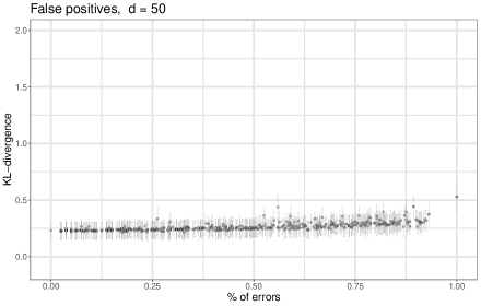
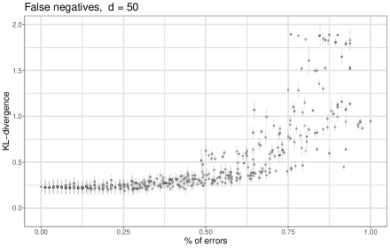
Figure 3: Error comparison for the proposed metric (x-axis) vs KL-divergence (y-axis) for synthetic datasets of 6 variables, and $s=50$. Top: % of false positives. Bottom: % of false negatives. Each dot in the graphs is a single structure.

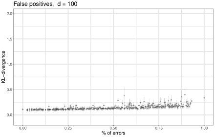
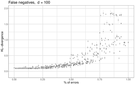
Figure 4: Error comparison for the proposed metric (x-axis) vs KL-divergence (y-axis) for synthetic datasets of 6 variables, and $s=100$. Top: % of false positives. Bottom: % of false negatives. Each dot in the graphs is a single structure.

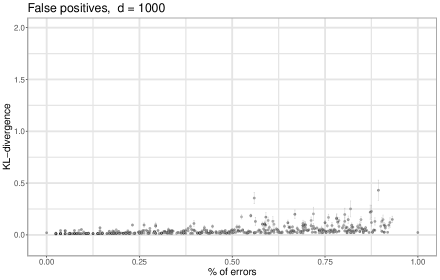
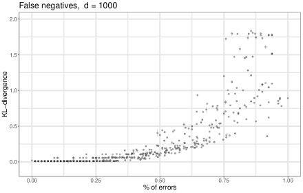
Figure 5: Error comparison for the proposed metric (x-axis) vs KL-divergence (y-axis) for synthetic datasets of 6 variables, and $s=1000$. Top: % of false positives. Bottom: % of false negatives. Each dot in the graphs is a single structure.

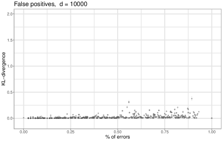
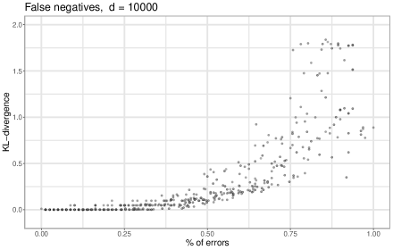
Figure 6: Error comparison for the proposed metric (x-axis) vs KL-divergence (y-axis) for synthetic datasets of 6 variables, and $s=10000$. Top: % of false positives. Bottom: % of false negatives. Each dot in the graphs is a single structure.

7.3 Conclusions of this comparison

A positive correlation between the KL-divergence and false negatives (as reported by our metric) can be observed. This is consistent with our knowledge, since this kind of errors are due to interactions that are missing from the structure, and therefore cannot be quantified by the parameters of the model, regardless of the amount of data. As a consequence, the KL-divergence shows the dissimilarity caused by the absence of interactions in the second model in relation to the first (original) model. Nevertheless, the KL-divergence does not correlate with false positives. In this case the measure over distributions can be said to conceal structural differences between models when the model to be compared possesses this kind of errors. On a final note, the amount of data serves as a confirmation of the above: as the amount of data used for parameter learning grows, the ability of the model‘s parameters to mitigate spurious interactions increases. This is caused by the compensation of the parameters, which becomes more accurate as more data are used to learn them.

8 Conclusions

In this paper we presented a metric for directly and efficiently comparing the structures of two log-linear models. These models are more expressive than undirected graphs due to their capacity to represent context-specific independencies. However, the interpretation of the independence structure of these models is complex, and no sound method for making direct quality comparisons of these structures was known to us prior to the design of our metric. The importance of a method that compares independence structures is that it can be used not only for enhancing the evaluation of structure learning algorithms, but also for qualitative comparisons in general. First and foremost, one can analyze differences in the independence structures learned with structure learning algorithms w.r.t. underlying synthetic structures, or compare the structures learned by different algorithms. Furthermore, one can draw qualitative insights about structures, either those learned by algorithms or those designed by human experts (or both), which cannot be obtained by mere observation except in simple (low-dimensional) scenarios.

Also, our method provides more guarantees than state-of-the-art techniques for assessing independence structures of log-linear models. On the one hand, for this representation, learning algorithms are usually evaluated with the KL-divergence measure for complete distributions, or the approximate method of CMLL for high dimensional domains, which require learning the numerical parameters of the models and are therefore indirect. Besides, they do not have the properties of a metric. On the other hand, some direct methods have been used, such as the average feature length or number of features, but these only provide very limited information about the structures, and no guarantees of their validity exist. In contrast, in this work we have proved that our technique is a metric, thus making it suitable for drawing reliable conclusions about comparisons made with it. Some possible future lines of research on this method may include the search for an efficient method w.r.t. the number of features in the models, and a reproduction of results from structure learning works, adding measurements with this new metric to the existing KL-divergence or CMLL scores, in order to analyze the impact of using our measure.

Appendix A Lemmas for the equivalent feature sets $H^{TP}$ and $H^{FN}$

This section contains the proofs for the sets proposed in Eqs. 37 and 41, in order to show that these sets correctly represent the context sets corresponding to $TP_{ij}$ and $FN_{ij}$, respectively, as defined in Theorem 1.

Proof.

From Aux. Lemma 2 and the definition of $H^{TP}(F,G)$, we have for the r.h.s. that

$$\mathcal{X}^{ij}({H^{TP}(F,G)}) =\bigcup_{h\in H^{TP}(F,G)}\mathcal{X}^{ij}({h})$$

$$=\bigcup_{{f}\cup^{ij}{g}\in H^{TP}(F,G)}\mathcal{X}^{ij}({{f}\cup^{ij}{g}})$$

$$=\bigcup_{f\sim C_{1}(f)}\,\,\,\bigcup_{g\sim C_{1}(g)\land C_{2}(f,g)}\mathcal{X}^{ij}({{f}\cup^{ij}{g}}),$$

where notation $a\sim c$ is used to denote the set of all elements $a$ satisfying condition $c$. For $f$ and $g$, the universe of elements is assumed to be $F$ and $G$, respectively. Thus, $f\sim C_{1}(f)$ denotes all features $f\in F$ satisfying condition $C_{1}(f)$, and $g\sim C_{1}(g)\land C_{2}(f,g)$ denotes all features $g\in G$ satisfying conditions $C_{1}(g)$ and $C_{2}(f,g)$.

It suffices then to prove that

$$\mathcal{X}^{ij}({F})\cap\mathcal{X}^{ij}({G})=\bigcup_{f\sim C_{1}(f)}\,\,\,\bigcup_{g\sim C_{1}(g)\land C_{2}(f,g)}\mathcal{X}^{ij}({{f}\cup^{ij}{g}})$$

For this purpose, we use the result of Aux. Lemma 2, stated and proven in C, and the set property of distribution of intersection over union, in the following manner:

$$\mathcal{X}^{ij}({F}) \cap\mathcal{X}^{ij}({G})$$

$$=\mathcal{X}^{ij}({F})\cap\left(\bigcup_{g\in G}\mathcal{X}^{ij}({g})\right) G$$ by  Aux. Lemma 2 over

$$=\bigcup_{g\in G}\mathcal{X}^{ij}({g})\cap\mathcal{X}^{ij}({F})$$ by distributive law

$$=\bigcup_{g\in G}\left(\mathcal{X}^{ij}({g})\cap\bigcup_{f\in F}\mathcal{X}^{ij}({f})\right) F$$ by  Aux. Lemma 2 over

$$=\bigcup_{g\in G}\bigcup_{f\in F}\mathcal{X}^{ij}({g})\cap\mathcal{X}^{ij}({f})$$ by distributive law.

To conclude, we use a result stated in  subsubsection 4.3.1, Section 4.3.1. According to this lemma, the intersections over individual features $\mathcal{X}^{ij}({f})\cap\mathcal{X}^{ij}({g})$ in the r.h.s. can be either empty, or equal to $\mathcal{X}^{ij}({{f}\cup^{ij}{g}})$; with the non-empty case occurring only if $f$ and $g$ satisfy conditions ${C}_{1}(f)$, ${C}_{1}(g)$, and ${C}_{2}(f,g)$. These conditions are precisely the restrictions stated in Eq. A, by which we can conclude that the equivalence is correct.

∎

Proof.

From Aux. Lemma 2 and the definition of $H^{FN}(F,G)$ we have for the r.h.s. that

$$\mathcal{X}^{ij}({H^{FN}(F,G)})= \bigcup_{h\in H^{FN}(F,G)}\mathcal{X}^{ij}({h})$$

$$= \left[\bigcup_{f\in F^{2}\setminus F^{1}}\,\bigcup_{D^{E}_{f}\in\Delta(f)}\mathcal{X}^{ij}\left({{f}\,\cup^{ij}\,\bigcup^{ij}_{d\in D^{E}_{f}}d}\right)\right]$$

$$\cup\left[\bigcup_{f\notin F^{1}\cup F^{2}}\,\bigcup_{D^{E}_{f}\in\Delta(f)}\mathcal{X}^{ij}\left({\bigcup^{ij}_{d\in D^{E}_{f}}d}\right)\right].$$ (58)

for $\Delta(f)=\bigtimes_{g\in G^{1}(f)\cup G^{2}(f)}D^{E}_{fg}$, a cross-product dependent on $f$, whose elements $D^{E}_{f}$ are sets of features of cardinality $|\overline{G^{1}(f)\cup G^{2}(f)}|$ computed by extracting exactly one feature from each $D^{E}_{fg}$, with one $D^{E}_{fg}$ defined per $g\notin G^{1}(f)\cup G^{2}(f)$

It suffices then to prove that $\mathcal{X}^{ij}({F})\setminus\mathcal{X}^{ij}({G})$ equals the r.h.s. of this last expression. We begin by applying a few set equivalences:

$$\mathcal{X}^{ij}({F}) \setminus\mathcal{X}^{ij}({G})$$

$$=\mathcal{X}^{ij}({F})\cap\overline{\mathcal{X}^{ij}({G})}$$ by general sets equivalence

$$=\overline{\mathcal{X}^{ij}({G})}\cap\bigcup_{f\in F}\mathcal{X}^{ij}({f}) F$$ by  Aux. Lemma 2 over

$$=\bigcup_{f\in F}\mathcal{X}^{ij}({f})\cap\overline{\mathcal{X}^{ij}({G})}$$ by distributive law

$$=\bigcup_{f\in F}\mathcal{X}^{ij}({f})\setminus\mathcal{X}^{ij}({G})$$ by general sets equivalence

$$=\bigcup_{f\in F}\mathcal{X}^{ij}({f})\setminus\bigcup_{g\in G}\mathcal{X}^{ij}({g}) G$$ by  Aux. Lemma 2 over

$$=\bigcup_{f\in F}\quad\bigcap_{g\in G}\mathcal{X}^{ij}({f})\setminus\mathcal{X}^{ij}({g})$$ by relative complements (59)

Specifically, the set equivalences used above are the following: the equivalence between subtracting a set and intersecting its complement (i.e., $A\setminus B=A\cap\overline{B}$), the property of distribution of intersection over union (e.g., $(A\cup B)\cap(C\cup D)=(A\cap C)\cup(A\cap D)\cup(B\cap C)\cup(B\cap D)$), and, in the last step, a property of sets known as relative complements that states that for sets $A$, $B$, and $C$, $C\setminus(A\cup B)=(C\setminus A)\cap(C\setminus B)$.

The resulting expression involves differences of FC context sets of individual features: $\mathcal{X}^{ij}({f})\setminus\mathcal{X}^{ij}({g})$. From Example 10 (Section 4.3.1), each of these differences can take one of three values, depending on the conditions that hold for each combination of $f$ and $g$:

$$\mathcal{X}^{ij}(f)\setminus\mathcal{X}^{ij}(g)\equiv\left\{\begin{array}[]{ll}\emptyset&\quad if~{}g^{ij}\subseteq f^{ij}\ \land C_{1}(g),\text{ or }\ \lnot C_{1}(f)\\[5.0pt] \mathcal{X}^{ij}({f})&\quad\lnot C_{2}(f,g)\ \text{or}\ \lnot C_{1}(g)\\[5.0pt] \bigcup_{d\in D^{E}_{fg}}\mathcal{X}^{ij}({d})&\quad otherwise.\end{array}\right.$$ (60)

We will now proceed to analyze the impact that the three possible values of the difference have in the union of intersections of Eq. 59. For that, we start by decomposing the intersection over $G$ over a partition of $G$ consisting of three parts: $g\in G^{1}(f)$, $g\in G^{2}(f)$, and the remainder $g\notin G^{1}(f)\cup G^{2}(f)$. Note the dependence on $f$ of the partition, indicating it is different for every $f$ of the union. The partition results in

$$\mathcal{X}^{ij}({F})\setminus\mathcal{X}^{ij}({G})\equiv\bigcup_{f\in F} \left\{\bigcap_{g\in G^{1}(f)}\mathcal{X}^{ij}({f})\setminus\mathcal{X}^{ij}({g})\,\,\,\bigcap_{g\in G^{2}(f)}\mathcal{X}^{ij}({f})\setminus\mathcal{X}^{ij}({g})\,\,\,\right.$$

$$\left.\bigcap_{g\notin G^{1}(f)\cup G^{2}(f)}\mathcal{X}^{ij}({f})\setminus\mathcal{X}^{ij}({g})\right\}$$

We shall start by the first partition over $g\in G^{1}(f)$. According to the definition of $G^{1}(f)$ in Eq. 42, any $g$ in it satisfies either $g^{ij}\subseteq f^{ij}\ \land C_{1}(g)$ or $\lnot C_{1}(f)$, which according to Eq. 60 is exactly the condition for the difference to be empty. Then, if for some $f\in F$ this condition holds for at least one $g\in G$, i.e., if $G^{1}(f)\neq\emptyset$, then the whole intersection over $G$ is empty, including all three partitions. From its definition in Eq. 42, this occurs for every $f\in F^{1}$. We can thus omit the partition over $G^{1}$ by simply restricting the union only over features $f\notin F^{1}$.

We will now analyze the second partition over $g\in G^{2}(f)$. According to the definition of $G^{2}(f)$ in Eq. 43, any $g$ in it satisfies either $\lnot C_{2}(f,g)$ or $\lnot C_{1}(g)$, which according to Eq. 60 is exactly the condition for the difference to be $\mathcal{X}^{ij}(f)$. This results in all differences within the intersection over the second partition to be $\mathcal{X}^{ij}(f)$.

Consequently, the intersection is now equal to $\mathcal{X}^{ij}(f)$. There is an exception to this, when no $g$ satisfies that condition for some $f$. This occurs when $G^{2}(f)=\emptyset$. When this happens, the second intersection can be ignored. From its definition in Eq. 43, this occurs for every feature $f$ that is not in $F^{2}$, resulting in a partition over $F$.

Combining the above conclusions, we have that

$$\mathcal{X}^{ij}({F})\setminus\mathcal{X}^{ij}({G})\equiv \left[\bigcup_{f\in F^{2}\setminus F^{1}}\mathcal{X}^{ij}({f})\bigcap_{g\notin G^{1}(f)\cup G^{2}(f)}\mathcal{X}^{ij}({f})\setminus\mathcal{X}^{ij}({g})\right]$$

$$\bigcup\left[\bigcup_{f\notin(F^{1}\cup F^{2})}\bigcap_{g\notin G^{1}(f)\cup G^{2}(f)}\mathcal{X}^{ij}({f})\setminus\mathcal{X}^{ij}({g})\right].$$

This leaves us with only the third partition to analyze. For that, we notice that all $g$ not in $G^{1}(f)$ nor $G^{2}(f)$ are exactly those not satisfying neither the first nor second condition but the third condition of Eq. 60. After replacing the difference by the expression corresponding to this third condition we obtain

$$\mathcal{X}^{ij}({F})\setminus\mathcal{X}^{ij}({G})\equiv \left[\bigcup_{f\in F^{2}\setminus F^{1}}\mathcal{X}^{ij}({f})\cap\left(\ \bigcap_{g\notin G^{1}(f)\cup G^{2}(f)}\,\,\bigcup_{d\in D^{E}_{fg}}\mathcal{X}^{ij}({d})\right)\right]$$

$$\bigcup\left[\bigcup_{f\notin(F^{1}\cup F^{2})}\bigcap_{g\notin G^{1}(f)\cup G^{2}(f)}\,\,\bigcup_{d\in D^{E}_{fg}}\mathcal{X}^{ij}({d})\right].$$

To continue, we further simplify the subexpression

$$\bigcap_{g\notin G^{1}(f)\cup G^{2}(f)}\bigcup_{d\in D^{E}_{fg}}\mathcal{X}^{ij}({d}),$$

which appears in both unions, by applying the distributive property of intersection over union to obtain

$$\mathcal{X}^{ij}({F})\setminus\mathcal{X}^{ij}({G})\equiv \left[\bigcup_{f\in F^{2}\setminus F^{1}}\quad\mathcal{X}^{ij}({f})\cap\left(\bigcup_{D^{E}_{f}\in\Delta(f)}\quad\bigcap_{d\in D^{E}_{f}}\mathcal{X}^{ij}(d)\right)\right]$$

$$\bigcup\left[\bigcup_{f\notin(F^{1}\cup F^{2})}\quad\bigcup_{D^{E}_{f}\in\Delta(f)}\quad\bigcap_{d\in D^{E}_{f}}\mathcal{X}^{ij}(d)\right].$$

for $\Delta(f)=\bigtimes_{g\in G^{1}(f)\cup G^{2}(f)}D^{E}_{fg}$, a cross-product dependent on $f$, whose elements $D^{E}_{f}$ are sets of features of cardinality $|\overline{G^{1}(f)\cup G^{2}(f)}|$ computed by extracting exactly one feature from each $D^{E}_{fg}$, with one $D^{E}_{fg}$ defined per $g\notin G^{1}(f)\cup G^{2}(f)$. To illustrate, if we assume that each $D^{E}_{fg}$ contains $2$ features, then the cross-product would produce $2^{|G^{1}(f)\cup G^{2}(f)|}$ features $D^{E}_{f}$, for each $f$.

One can also apply the distribution of intersection over union of $\mathcal{X}^{ij}({f})$ onto the union over the $D^{E}_{f}$, to obtain

$$\mathcal{X}^{ij}({F})\setminus\mathcal{X}^{ij}({G})\equiv \left[\bigcup_{f\in F^{2}\setminus F^{1}}\quad\bigcup_{D^{E}_{f}\in\Delta(f)}\quad\left(\mathcal{X}^{ij}({f})\cap\bigcap_{d\in D^{E}_{f}}\mathcal{X}^{ij}(d)\right)\right]$$

$$\bigcup\left[\bigcup_{f\notin(F^{1}\cup F^{2})}\quad\bigcup_{D^{E}_{f}\in\Delta(f)}\quad\bigcap_{d\in D^{E}_{f}}\mathcal{X}^{ij}(d)\right].$$

To conclude the proof, we note that the intersection of the FC sets of $f$ and the $d$ in $D^{E}_{f}$ corresponds to the non-empty case from Eq. 46 in subsubsection 4.3.1; therefore, it can be replaced by the union of features over $(i,j)$, resulting in

$$\mathcal{X}^{ij}({F})\setminus\mathcal{X}^{ij}({G})\equiv \left[\bigcup_{f\in F^{2}\setminus F^{1}}\quad\bigcup_{D^{E}_{f}\in\Delta(f)}\quad\mathcal{X}^{ij}\left(f\cup^{ij}\bigcup^{ij}_{d\in D^{E}_{f}}{d}\right)\right]$$

$$\bigcup\left[\bigcup_{f\notin(F^{1}\cup F^{2})}\quad\bigcup_{D^{E}_{f}\in\Delta(f)}\quad\mathcal{X}^{ij}\left(\bigcup^{ij}_{d\in D^{E}_{f}}{d}\right)\right].$$

The above expression matches exactly what Eq. A indicated is sufficient for proving the lemma. ∎

Appendix B Lemmas for the efficient computation of $\mathcal{X}^{ij}({f})\cap\mathcal{X}^{ij}({g})$ and $\mathcal{X}^{ij}({f})\setminus\mathcal{X}^{ij}({g})$

This appendix provides the proofs for subsubsection 4.3.1 and Example 10 of Section 4.3.1, which propose an approach for the efficient computation of the intersection $\mathcal{X}^{ij}({f})\cap\mathcal{X}^{ij}({g})$ and difference $\mathcal{X}^{ij}({f})\setminus\mathcal{X}^{ij}({g})$ of the FC context sets of single features, respectively.

Proof.

We will consider each case separately.

Case $\lnot C_{1}(f)$: By the definition of this condition, $X_{i}\notin S_{f}$ or $X_{j}\notin S_{f}$. This contradicts the r.h.s. in  Aux. Lemma 1 (see  C), which implies that there is no $x_{Z}\in\mathcal{X}^{ij}({f})$, or equivalently, $\mathcal{X}^{ij}(f)=\emptyset$. This in turn implies an empty intersection.

Case $\lnot C_{1}(g)$: The case of $C_{1}(f)$ applies here as well, resulting in $\mathcal{X}^{ij}(g)=\emptyset$, and therefore in an empty intersection.

Case $\lnot C_{2}(f,g)$: For this case, neither $\mathcal{X}^{ij}(f)$ nor $\mathcal{X}^{ij}(g)$ are empty, but their intersection is. To prove this, we argue that given any two FC contexts $x_{Z}\in\mathcal{X}^{ij}(f)$ and $x_{Z}^{\prime}\in\mathcal{X}^{ij}(g)$, they must differ in the assignment of at least one of its variables. By the definition of $C_{2}(f,g)$ in Eq. 40, its negation implies that there exists at least one variable $X_{h}$ other than $X_{i}$ and $X_{j}$ that is both in $f$ and $g$, such that $X_{h}(f)\neq X_{h}(g)$. According to Eq. 76 of Aux. Lemma 1 (see C), we have that, for all $x_{Z}\in\mathcal{X}^{ij}({f})$, $X_{h}(x_{Z})=X_{h}(f)$, while for all $x^{\prime}_{Z}\in\mathcal{X}^{ij}({g})$, $X_{h}(x^{\prime}_{Z})=X_{h}(g)$. Therefore, for all $x_{Z}\in\mathcal{X}^{ij}({f})$ and all $x^{\prime}_{Z}\in\mathcal{X}^{ij}({g})$, we have $X_{h}(x_{Z})\neq X_{h}(x^{\prime}_{Z})$ which implies $x_{Z}\neq x^{\prime}_{Z}$, by which we conclude that no FC context belongs to both $\mathcal{X}^{ij}({f})$ and $\mathcal{X}^{ij}({g})$ simultaneously.

Case $C_{1}(f)\land C_{1}(g)\land C_{2}(f,g)$ : We must prove that $\mathcal{X}^{ij}(f)\cap\mathcal{X}^{ij}(g)\equiv\mathcal{X}^{ij}(f\cup{g}^{ij})$. In what follows, we denote by $x_{Z}$ an arbitrary FC context in $\mathcal{X}^{ij}$. From basic set theory, we have that

$$x_{Z}\in\mathcal{X}^{ij}(f)\cap\mathcal{X}^{ij}(g)\iff x_{Z}\in\mathcal{X}^{ij}({f})\land x_{Z}\in\mathcal{X}^{ij}({g}).$$

By applying  Aux. Lemma 1 to the conditions in the r.h.s. we obtain

$$x_{Z}\in\mathcal{X}^{ij}(f)\cap\mathcal{X}^{ij}(g)\iff{f}^{ij}\subseteq x_{Z}\,\,\,\land\,\,\,{g}^{ij}\subseteq x_{Z}\,\,\,\land\,\,\,X_{i},X_{j}\in S_{f}\,\,\,\land\,\,\,X_{i},X_{j}\in S_{g}.$$

From set theory, we know that for arbitrary sets $A$, $B$, and $C$, $A\subseteq C\land B\subseteq C$ is equivalent to $A\cup B\subseteq C$. This applies in particular to the union of features (Definition 1), as the union ${f}^{ij}\cup{g}^{ij}$ is a feature that contains all assignments in both features, and by the r.h.s., all of these assignments are in $x_{Z}$. Also, from the definition of feature union, if $X_{i},X_{j}$ are in the scopes of both $f$ and $g$, then they are in the scope of their union. Combining both conclusions, we obtain

$$x_{Z}\in\mathcal{X}^{ij}(f)\cap\mathcal{X}^{ij}(g)\iff{f}^{ij}\cup{g}^{ij}\subseteq x_{Z}\,\,\,\land\,\,\,X_{i},X_{j}\in S_{f\cup g}.$$

To conclude the proof we apply the right-to-left direction of Eq. 76 (Aux. Lemma 1), where the feature ${f}^{ij}\cup{g}^{ij}={h}^{ij}$ should have a corresponding feature $h$ in the l.h.s. of Eq. 76, that is, a feature that contains $X_{i}$ and $X_{j}$ in its scope. Note that the l.h.s. of the auxiliary lemma holds for any arbitrary assignment to this pair of variables; then, by Definition 2, such a feature can be expressed as a union over the pair $(i,j)$, namely, $f\cup^{ij}g$, which allows us to obtain

$$x_{Z}\in\mathcal{X}^{ij}(f)\cap\mathcal{X}^{ij}(g)\iff x_{Z}\in\mathcal{X}^{ij}({f\cup^{ij}{g}}).$$

∎

We will now prove the following lemma for the difference of the FC contexts of single features.

Proof.

For the first case of Eq. 47, we consider the two cases of the disjunction in the condition separately:

$\lnot C_{1}(f)$: If this is the case, the right-hand side of  Aux. Lemma 1 never holds. This results in $\mathcal{X}^{ij}(f)=\emptyset$, and consecuently the difference is empty.

${g}^{ij}\subseteq{f}^{ij}\land C_{1}(g)$: For this case we prove the difference is empty by showing that $\mathcal{X}^{ij}({f})\subseteq\mathcal{X}^{ij}({g})$, which means that for every $x_{Z}\in\mathcal{X}^{ij}$ it is the case that

$$x_{Z}\in\mathcal{X}^{ij}({f})\implies x_{Z}\in\mathcal{X}^{ij}({g})$$

From the left-hand side and  Aux. Lemma 1, we have that ${f}^{ij}\subseteq x_{Z}\land{C}_{1}(f)$, which combined with condition ${g}^{ij}\subseteq{f}^{ij}$ results in ${g}^{ij}\subseteq x_{Z}$. The latter combined with $C_{1}(g)$ can be applied to the left-to-right implication of Eq. 76 of the auxiliary lemma to obtain $x_{Z}\in\mathcal{X}^{ij}({g})$.

For the second case of Eq. 47, if $\lnot C_{2}(f,g)$ holds, some value in $g$ does not match its corresponding value in $f$, and therefore none of the elements of $\mathcal{X}^{ij}(g)$ are in $\mathcal{X}^{ij}(f)$. If $\lnot C_{1}(g)$ holds, then $\mathcal{X}^{ij}(g)=\emptyset$. In both cases, nothing can be subtracted from $\mathcal{X}^{ij}(f)$.

The proof for the third case of Eq. 47 consists in proving that, when the conditions of the first two cases are not satisfied, then

$$\mathcal{X}^{ij}({f})\setminus\mathcal{X}^{ij}({g})=\bigcup_{d\in D^{E}_{fg}}{\mathcal{X}^{ij}({d})}.$$

For that we proceed in two steps. First, we prove this equality for $D_{fg}$, an alternative (simpler) version of $D^{E}_{fg}$, i.e.,

$$\mathcal{X}^{ij}({f})\setminus\mathcal{X}^{ij}({g})=\bigcup_{d\in D_{fg}}{\mathcal{X}^{ij}({d})}.$$ (61)

where the equivalent set $D_{fg}$ is defined as

$$D_{fg}=\left\{\text{\ features }d\ \middle|\begin{array}[]{l}S_{d}=S_{f}\cup S_{g};\forall X_{m}\in S_{f},X_{m}(d)=X_{m}(f);\\ \exists X_{k}\in S_{g}\setminus S_{f},X_{k}(d)\neq X_{k}(g)\end{array}\right\}.$$ (62)

that is, one feature $d$ with scope composed of all variables in the scopes of both $f$ and $g$, with matching values with those in $S_{f}$, and a mistmatch with at least one variable in $S_{g}$.

Then, we prove that $D_{fg}$ is equivalent to $D^{E}_{fg}$:

$$\bigcup_{d\in D_{fg}}{\mathcal{X}^{ij}({d})}=\bigcup_{d\in D^{E}_{fg}}{\mathcal{X}^{ij}({d})},$$

The validity of these two steps is proven below in Lemmas 1 and 2, respectively. Additionally, we include  Lemma 3, which shows that the FC contexts of each feature in $D^{E}_{fg}$ are mutually exclusive, which guarantees that redundancy is conveniently reduced, and is necessary for Algorithm 1 to produce a correct result.

∎

Lemma 1.

Let $X_{i}$ and $X_{j}$ be two distinct variables in $X_{V}$, and let $f$ and $g$ be two arbitrary features over $X_{V}$ satisfying neither the first nor second conditions of Eq. 47. Then,

$$\mathcal{X}^{ij}({f})\setminus\mathcal{X}^{ij}({g})=\bigcup_{d\in D_{fg}}{\mathcal{X}^{ij}({d})}.$$ (61)

with $D_{fg}$ defined as in Eq. 62.

Proof.

By set equivalence, Eq. 61 can be reformulated, for an arbitrary $x_{Z}\in\mathcal{X}^{ij}$, as

$$x_{Z}\in\mathcal{X}^{ij}({f})\land x_{Z}\notin\mathcal{X}^{ij}({g})\iff\exists d\in D_{fg},x_{Z}\in\mathcal{X}^{ij}({d}).$$

Since the first and second cases in Eq. 47 are not satisfied, we have that ${g}^{ij}\not\subseteq{f}^{ij}$, $C_{2}(f,g)$, $C_{1}(f)$, and $C_{1}(g)$; this is easily demonstrated by the simple application of logical equivalences over the negation of the first two conditions.

Then, applying  Aux. Lemma 1 of  C to each of the three inclusions $x_{Z}\in\mathcal{X}^{ij}({f})$, $x_{Z}\in\mathcal{X}^{ij}({g})$, and $x_{Z}\in\mathcal{X}^{ij}({d})$ we obtain

$$\left(C_{1}(f)\land{f}^{ij}\subseteq x_{Z}\right)\land\left(\lnot C_{1}(g)\lor{g}^{ij}\not\subseteq x_{Z}\right)\iff\exists d\in D_{fg},\ \left(C_{1}(d)\land{d}^{ij}\subseteq x_{Z}\right).$$ (63)

We begin with the right-to-left implication, and prove each term in the l.h.s. separately, i.e.,

1. $\exists d\in D_{fg},\left(C_{1}(d)\land{d}^{ij}\subseteq x_{Z}\right)\implies\left(C_{1}(f)\land{f}^{ij}\subseteq x_{Z}\right)$; and

2. $\exists d\in D_{fg},\left(C_{1}(d)\land{d}^{ij}\subseteq x_{Z}\right)\implies\left(\lnot C_{1}(g)\lor{g}^{ij}\not\subseteq x_{Z}\right)$.

1. Since $S_{d}=S_{f}\cup S_{g}$ and both $C_{1}(f)$ and $C_{1}(g)$ hold, then $C_{1}(d)$ holds as well. It then suffices to prove $\exists d\in D_{fg},{d}^{ij}\subseteq x_{Z}\implies{f}^{ij}\subseteq x_{Z}$.

   For that, we use  Aux. Lemma 3. We consider $a=f^{ij}$ and $b=d^{ij}$, where $d$ is the feature satisfying the l.h.s. of (i), i.e., the feature $d$ for which $d^{ij}\subseteq x_{Z}$. We thus have that $b\subseteq x_{Z}$. To conclude that $a=f^{ij}\subseteq x_{Z}$ it suffices then to prove that $f^{ij}\subseteq d^{ij}$ and that $S_{f}\subseteq S_{d}$. By definition, $S_{d}=S_{f}\cup S_{g}$, so $S_{f}\subseteq S_{d}$ holds. Also, by definition, for every $k\in D_{fg}$, it is the case that $\forall X_{m}\in S_{f^{ij}},X_{m}(k)=X_{m}(f^{ij})$, which is equivalent to saying that for every $k\in D_{fg}$, ${f}^{ij}\subseteq{k}^{ij}$. In particular, this must then hold for $d$. ∎

2. Again, $C_{1}(d)$ holds. Also, since we already know that $C_{1}(g)$, the r.h.s. reduces to ${g}^{ij}\not\subseteq x_{Z}$. It thus suffices to prove that $\exists d\in D_{fg},{d}^{ij}\subseteq x_{Z}\implies{g}^{ij}\not\subseteq x_{Z}$.

   To prove this we first note that

   $$d^{ij}\subseteq x_{Z}\implies\forall X_{m}\in S_{d^{ij}},X_{m}(d^{ij})=X_{m}(x_{Z}).$$ (64)

   Then, from the definition of every $d\in D_{fg}$, $\exists X_{m}\in S_{g}\setminus S_{f}$ s.t. $X_{m}(d)\neq X_{m}(g)$. Also, since both $X_{i}$ and $X_{j}$ are in $S_{f}$, then $S_{g}\setminus S_{f}=S_{g^{ij}}\setminus S_{f^{ij}}$, so $\exists X_{m}\in S_{g^{ij}}\setminus S_{f^{ij}}$ s.t. $X_{m}(d^{ij})\neq X_{m}(g^{ij})$. Combining with Eq. 64, this results in $\exists X_{m}\in S_{g^{ij}}\setminus S_{f^{ij}}$ s.t. $X_{m}(g^{ij})\neq X_{m}(x_{Z})$, from which we can conclude that $g^{ij}\not\subseteq x_{Z}$.

   ∎

We proceed now to prove the left-to-right implication of Eq. 63. For that, it suffices to consider the l.h.s. without terms $C_{1}(f)$ and $\lnot C_{1}(g)$. The former can be omitted because it is a condition of the lemma that $C_{1}(f)$, while the latter can be omitted because again, it is a condition of the lemma that $C_{1}(g)$, i.e., $\lnot C_{1}(g)$ is false, so for the disjunction to be true it must be that ${g}^{ij}\not\subseteq x_{Z}$. Finally, we already showed above that $C_{1}(d)$. It thus suffices to prove that:

$${f}^{ij}\subseteq x_{Z}\land{g}^{ij}\not\subseteq x_{Z}\implies\exists d\in D_{fg},{d}^{ij}\subseteq x_{Z},$$

that is, given the condition on the l.h.s. for any arbitrary $x_{Z}$, there is some $d\in D_{fg}$ for which the r.h.s. is satisfied, i.e., ${d}^{ij}\subseteq x_{Z}$.

We start by reinterpreting the l.h.s.:

$(f^{ij}\subseteq x_{Z}):$

$$(f^{ij}\subseteq x_{Z}):\forall X_{m}\in S_{f^{ij}},X_{m}(f^{ij})=X_{m}(x_{Z}).$$ (65)

$(g^{ij}\not\subseteq x_{Z}):$

Since $S_{x_{Z}}=V\setminus\{X_{i},X_{j}\}$ and $S_{g}^{ij}\subseteq S_{x_{Z}}$, then $g^{ij}\not\subseteq x_{Z}$ can only occur because some assignment in $g^{ij}$ takes a value that is different from $x_{Z}$, i.e.,

$$\exists X_{m}\in S_{g^{ij}}\text{ s.t. }X_{m}(g^{ij})\neq X_{m}(x_{Z}).$$ (66)

Nevertheless, by Eq. 65 and $C_{2}(f,g)$, this cannot be the case for all $X_{m}\in S_{g^{ij}}\cap S_{f^{ij}}$ so Eq. 66 can be re-expressed as

$$\exists X_{m}\in S_{g^{ij}}\setminus S_{f^{ij}}\text{ s.t. }X_{m}(g^{ij})\neq X_{m}(x_{Z}).$$ (67)

Finally, since $C_{1}(f)$ holds, both $X_{i}$ and $X_{j}$ are in $S_{f}$, so $S_{g^{ij}}\setminus S_{f^{ij}}=Sg\setminus S_{f}$, i.e., Eq. 67 becomes

$$\exists X_{m}\in S_{g}\setminus S_{f},X_{m}(g^{ij})\neq X_{m}(x_{Z}).$$ (68)

Let $M$ denote those $X_{m}$ that satisfy Eq. 68, i.e.,

$$\forall X_{m}\in M,X_{m}(g^{ij})\neq X_{m}(x_{Z}).$$ (69)

We proceed by proposing some feature $d$ defined over $S_{f}\cup S_{g}$ that satisfies $d^{ij}\subseteq x_{Z}$, .i.e,

$$\forall X_{m}\in S_{d}^{ij}=S_{f}\cup S_{g},~{}X_{m}(d)=X_{m}(x_{Z}),$$ (70)

and prove that $d\in D_{fg}$. For that, we prove that $d$ satisfies all three conditions in the definition of any $d\in D_{fg}$:

1. The first condition, $S_{d}=S_{f}\cup S_{g}$ is satisfied by the definition of $d$.

2. From Eqs. 65 and 70, and the fact that $S_{f^{ij}}\subseteq S_{d}$ (by definition of $d$), we have that $\forall X_{m}\in S_{f^{ij}},X_{m}(f^{ij})=X_{m}(x_{Z})=X_{m}(d)$, satisfying the second condition of $D_{fg}$ for $X_{m}(f^{ij})$ and $X_{m}(d)$.

3. From Eqs. 69 and 70, and the fact that $M\subseteq S_{g}\setminus S_{f}$ (by definition of $M$), and $S_{g}\setminus S_{f}\subseteq S_{d}$ (by definition of $d$), and consequently $M\subseteq S_{d}$, we have that

   $$\forall X_{m}\in M,X_{m}(g^{ij})\neq X_{m}(x_{Z})=X_{m}(d),$$

   then $\forall X_{m}\in M,X_{m}(d)\neq X_{m}(g^{ij})$, satisfying the third condition of $D_{fg}$.

∎

Lemma 2.

$$\bigcup_{d\in D_{fg}}{\mathcal{X}^{ij}({d})}=\bigcup_{d\in D^{E}_{fg}}{\mathcal{X}^{ij}({d})}.$$ (71)

for $D^{E}_{fg}$ defined by Eq. 48 and $D_{fg}$ defined by Eq. 62.

Proof.

For arbitrary $x_{Z}$, Eq. 71 is equivalent to

$$\exists d\in D_{fg},~{}x_{Z}\in\mathcal{X}^{ij}({d})\iff\exists d^{\prime}\in D^{E}_{fg},x_{Z}\in\mathcal{X}^{ij}({d^{\prime}}).\\$$

Since $C_{1}(f)$, $S_{f}\subseteq S_{d}$ and $S_{f}\subseteq S_{d^{\prime}}$, we have that both $X_{i}$ and $X_{j}$ are in both $S_{d}$ and $S_{d^{\prime}}$, and therefore it holds that $C_{1}(d)$ and $C_{1}(d^{\prime})$. We can then apply Eq. 76 to the above to obtain

$$\exists d\in D_{fg},~{}d\subseteq x_{Z}\iff d\in D^{E}_{fg},d\subseteq x_{Z}.$$ (72)

For the left-to-right implication, by  Aux. Lemma 1, it suffices to prove that

$$\exists d\in D_{fg}\land\exists d^{\prime}\in D^{E}_{fg}\text{ s.t. }d^{\prime}\subseteq d,$$ (73)

for $a=d^{\prime},b=d$. Any $d^{\prime}\in D^{E}_{fg}$ and $d\in D_{fg}$ satisfy $S_{f}\subseteq S_{d^{\prime}}$ and $S_{f}\subseteq S_{d}$, respectively, and match the values of $f^{ij}$, so to prove $d^{\prime}\subseteq d$ we can focus on the values for $g$. For that, we start noticing that every feature $d^{\prime}\in D^{E}_{fg}$ is defined over some subset of $S_{g}\setminus S_{f}$ (dependent on $k$), over which it is guaranteed to have an assignment different from that of $g$ at $k$, i.e., $X_{k}(d^{\prime})\neq X_{k}(g)$. Then, any $d$ satisfying these assignments for these variables in $S_{d^{\prime}}\setminus S_{f}\ =S_{{d}^{ij}}^{\leq k}\setminus S_{f}$, and any value for the remaining assignments in $S_{g}\setminus S_{f}$ would satisfy that $\exists X_{m}\in S_{g}\setminus S_{f},X_{m}(d)\neq X_{m}(g)$, and thus is in $D_{fg}$.

For the right-to-left implication of Eq. 72, we have that, by Eq. 73, for every $d^{\prime}\in D^{E}_{fg}$ there exists a $d\in D_{fg}$ such that $d^{\prime}\subseteq d$. It suffices then to complete $d^{\prime}$ with assignments for the remaining variables with values matching $x_{Z}$, i.e.,

$$\forall X_{k}\in S_{{g}^{ij}}^{>k}\setminus S_{f},X_{k}(d)=X_{k}(x_{Z}).$$ (74)

Then, by Eq. 74 and the fact that $d^{\prime}\subseteq x_{Z}$, we conclude that $d\subseteq x_{Z}$.

∎

Lemma 3.

The FC contexts for each feature in $D^{E}_{fg}$ are mutually exclusive:

$$\forall d,d^{\prime}\in D^{E}_{fg},\mathcal{X}^{ij}({d})\cap\mathcal{X}^{ij}({d^{\prime}})=\emptyset$$ (75)

Proof.

Given the definition of $D^{E}_{fg}$ in Eq. 49, all features $d$ in some ${D^{E}_{fg}}_{(k)}$ have different values at $X_{k}$ among each other, by which they cannot have FC contexts in common. Additionally, for another $k^{\prime}$ such that $k^{\prime}>k$, not only are the FC contexts of the features mutually exclusive among each other, but they are also different from all features for the previous index $k$, since these features take values different from $X_{k}(g)$ at $X_{k}$, while features at $k^{\prime}$ have the value $X_{k}(g)$ at $X_{k}$.

∎

Appendix C Auxiliary lemmas

Auxiliary Lemma 1.

Let $F$ be the log-linear model of some distribution over $X_{V}$, $f\in F$ be some feature in $F$, let $X_{i},X_{j}\in S_{f}$ be two different variables in the scope of $f$, $x_{Z}\in\mathcal{X}^{ij}$ be some FC context, and ${f}^{ij}$ denote the feature composed of the same assignments in $f$ except for those of $X_{i}$ and $X_{j}$. Then,

$$x_{Z}\in\mathcal{X}^{ij}(f)\iff{f}^{ij}\subseteq x_{Z}\land X_{i},X_{j}\in S_{f},$$ (76)

where the subset operation ${f}^{ij}\subseteq x_{Z}$ runs over assignments, that is, it reads that every variable in feature $f$ other than $X_{i}$ and $X_{j}$ is assigned to the same value in both ${f}^{ij}$ and $x_{Z}$.

Proof.

This auxiliary lemma is a straight rewrite of known facts from the theory of log-linear models. From the definition of $\mathcal{X}^{ij}(f)$ in Eq. 22, $x_{Z}\in\mathcal{X}^{ij}(f)$ whenever $(X_{i}\mbox{$\perp\!\!\!\!\perp\!\!\!\!\!\not~{}~{}~{}$}X_{j}\mid x_{Z})_{F}$. According to [Chapter 4, [4]], any distribution structured by some log-linear model $F$, holds a direct interaction (a dependency) among any pair of variables $X_{i}$ and $X_{j}$, whenever they appear together in at least one feature $f\in F$. Moreover, the interaction still holds when conditioned on some partial assignment of variables, when there is at least one feature $f\in F$ satisfying that all its assignments match the conditioning set. In particular, for the case of FC conditioning sets, $I({X_{i}},{X_{j}}\mid x_{Z})$ is false (dependency) whenever each variable in $x_{Z}$ (which is also in the scope $S_{f}$) has a matching value in both. The auxiliary lemma is proven after noticing that $x_{Z}$ contains neither $X_{i}$ nor $X_{j}$.

∎

Auxiliary Lemma 2.

The FC set $\mathcal{X}^{ij}({F})$ of a log-linear model $F$ is equivalent to the union of the FC sets $\mathcal{X}^{ij}({f})$ of each of its features $f\in F$; formally,

$$\mathcal{X}^{ij}({F})=\bigcup_{f\in F}\mathcal{X}^{ij}({f}).$$

Before proceeding to the proof, we will illustrate this definition with an example:

Example 12.

Let $V=\{1,\dots,4\}$, $\forall X_{k},val(X_{k})=\{0,1\}$, and let $f,f^{\prime},f^{\prime\prime}\in F$ where

$$f= <X_{1}=0,X_{3}=0,X_{4}=1>,$$

$$f^{\prime}= <X_{2}=1,X_{3}=0,X_{4}=0>,\ and$$

$$f^{\prime\prime}= <X_{1}=0,X_{2}=0>.$$

Let $i=3$ and $j=4$. Then,

$$\mathcal{X}^{34}(f)= \ \{<X_{1}=0,X_{2}=0>,<X_{1}=0,X_{2}=1>\}$$

$$\mathcal{X}^{34}(f^{\prime})= \ \{<X_{1}=0,X_{2}=1>,<X_{1}=1,X_{2}=1>\}$$

$$\mathcal{X}^{34}(f^{\prime\prime})= \ \emptyset.$$

Then, $\mathcal{X}^{34}(F)$ is the union of the sets of FC contexts $\mathcal{X}^{34}(f)$ and $\mathcal{X}^{34}(f^{\prime})$, assuming $f$ and $f^{\prime}$ are the only features in $F$ containing $X_{3}$ and $X_{4}$ in their scope, resulting in

$$\mathcal{X}^{34}(F)= \mathcal{X}^{34}(f)\cup\mathcal{X}^{34}(f^{\prime})$$

$$= \{<X_{1}=0,X_{2}=0>,<X_{1}=0,X_{2}=1>,<X_{1}=1,X_{2}=1>\}.$$

Proof.

From Eq 22, $\mathcal{X}^{ij}(F)\equiv\{x_{Z}\in\mathcal{X}^{ij}~{}\mid~{}(X_{i}\mbox{$\perp\!\!\!\!\perp\!\!\!\!\!\not~{}~{}~{}$}X_{j}\mid x_{Z})_{F}\}$; also, by the same reasoning followed in  Aux. Lemma 1, if an assertion $I({X_{i}},{X_{j}}\mid x_{Z})$ is false (dependency) according to some feature $f\in F$, it is false according to the complete log-linear model:

$$(X_{i}\mbox{$\perp\!\!\!\!\perp\!\!\!\!\!\not~{}~{}~{}$}X_{j}\mid x_{u},X_{W})_{f}\implies(X_{i}\mbox{$\perp\!\!\!\!\perp\!\!\!\!\!\not~{}~{}~{}$}X_{j}\mid x_{u},X_{W})_{F}.$$

Therefore,

$$\mathcal{X}^{ij}(F) \equiv \{x_{Z}\in\mathcal{X}^{ij}~{}\mid~{}(X_{i}\mbox{$\perp\!\!\!\!\perp\!\!\!\!\!\not~{}~{}~{}$}X_{j}\mid x_{Z})_{F}\}$$

$$\equiv \{x_{Z}\in\mathcal{X}^{ij}~{}\mid~{}\vee_{f\in F}(X_{i}\mbox{$\perp\!\!\!\!\perp\!\!\!\!\!\not~{}~{}~{}$}X_{j}\mid x_{Z})_{f}\}$$

$$\equiv \bigcup_{f\in F}\left\{x_{Z}\in\mathcal{X}^{ij}~{}\mid~{}(X_{i}\mbox{$\perp\!\!\!\!\perp\!\!\!\!\!\not~{}~{}~{}$}X_{j}\mid x_{Z})_{f}\right\}$$

$$\equiv \bigcup_{f\in F}\mathcal{X}^{ij}({f})$$

∎

Auxiliary Lemma 3.

Let $a$ and $b$ be two features such that $S_{a}\subseteq S_{b}$, and $a\subseteq b$, then $b\subseteq x_{Z}\implies a\subseteq x_{Z}$.

Proof.

$$a\subseteq b\implies\forall k\in S_{a},X_{k}(a)=X_{k}(b),$$ (77)

then,

$$\begin{array}[]{ll}b\subseteq x_{Z}&\ \implies\forall k\in S_{b}X_{k}(b)=X_{k}(x_{Z})\\ &\ \implies\forall k\in S_{a}X_{k}(b)=X_{k}(x_{Z})\text{, by }S_{a}\subseteq S_{b}\\ &\ \implies\forall k\in S_{a}X_{k}(a)=X_{k}(x_{Z})\text{, by Eq.~{}\ref{eq:alsubset}}\\ &\ \implies a\subseteq x_{Z}.\end{array}$$

∎

Funding

This work was supported by CONICET (Argentinean Council for Scientific and Technological Research) [full doctoral scholarship for Jan Strappa]; and Universidad Tecnológica Nacional [grant EIUTIME0004481TC].

Data availability

The source code used for computing the metric for the simulation presented in Section 7 is available in Figshare at https://dx.doi.org/10.6084/m9.figshare.14666163. The implementation used for computing the KL-divergence is also available in Figshare at https://dx.doi.org/10.6084/m9.figshare.14668473.

The log-linear models‘ files are the same from [ederaSchluterBromberg14] and were provided by its corresponding author with permission. These data may be shared on request to the corresponding author of the cited work.

The Libra Toolkit is available at http://libra.cs.uoregon.edu/.

Other data and source code related to this simulation will be shared on reasonable request to the corresponding author.

References

- Christensen [2006] Ronald Christensen. Log-Linear Models and Logistic Regression. Springer-Verlag, New York, 2006.
- Agresti [2002] A. Agresti. Categorical Data Analysis. John Wiley & Sons, Hoboken, New Jersey, second edition, 2002.
- Haberman [1973] Shelby J. Haberman. Log-Linear Models for Frequency Data: Sufficient Statistics and Likelihood Equations. The Annals of Statistics, 1(4):617–632, July 1973. ISSN 0090-5364, 2168-8966. doi: 10.1214/aos/1176342458.
- Koller and Friedman [2009] D. Koller and N. Friedman. Probabilistic Graphical Models: Principles and Techniques. MIT Press, Cambridge, MA, 2009.
- Lauritzen [1996] S. Lauritzen. Graphical Models. Oxford University Press, Oxford, 1996.
- Shah et al. [2018] Rushabh Shah, Elizabeth Wilkins, Melanie Nichols, Paul Kelly, Farah El-Sadi, F Lucy Wright, and Nick Townsend. Epidemiology report: trends in sex-specific cerebrovascular disease mortality in Europe based on WHO mortality data. European Heart Journal, 40(9):755–764, Aug 2018. doi: 10.1093/eurheartj/ehy378. URL https://doi.org/10.1093%2Feurheartj%2Fehy378.
- Yuan et al. [2021] Jie Yuan, Yu Wu, Wenzhan Jing, Jue Liu, Min Du, Yaping Wang, and Min Liu. Non-linear correlation between daily new cases of COVID-19 and meteorological factors in 127 countries. Environmental Research, 193:110521, Feb 2021. doi: 10.1016/j.envres.2020.110521. URL https://doi.org/10.1016%2Fj.envres.2020.110521.
- Panagiotakos and Pitsavos [2021] Demosthenes B. Panagiotakos and Christos Pitsavos. Interpretation of epidemiological data using multiple correspondence analysis and log-linear models. Journal of Data Science, 2(1):75–86, Jul 2021. doi: 10.6339/jds.2004.02(1).122. URL https://doi.org/10.6339%2Fjds.2004.02%281%29.122.
- Lundtofte and Wilhelmsson [2013] Frederik Lundtofte and Anders Wilhelmsson. Risk premia: Exact solutions vs. log-linear approximations. Journal of Banking & Finance, 37(11):4256–4264, 2013. ISSN 0378-4266. doi: https://doi.org/10.1016/j.jbankfin.2013.07.035. URL https://www.sciencedirect.com/science/article/pii/S0378426613003105.