Spectral Graph Matching and Regularized Quadratic Relaxations II: Erdős-Rényi Graphs and Universality

Abstract

We analyze a new spectral graph matching algorithm, GRAph Matching by Pairwise eigen-Alignments (GRAMPA), for recovering the latent vertex correspondence between two unlabeled, edge-correlated weighted graphs. Extending the exact recovery guarantees established in the companion paper [FMWX19] for Gaussian weights, in this work, we prove the universality of these guarantees for a general correlated Wigner model. In particular, for two Erdős-Rényi graphs with edge correlation coefficient $1-\sigma^{2}$ and average degree at least $\operatorname{polylog}(n)$, we show that GRAMPA exactly recovers the latent vertex correspondence with high probability when $\sigma\lesssim 1/\operatorname{polylog}(n)$. Moreover, we establish a similar guarantee for a variant of GRAMPA, corresponding to a tighter quadratic programming relaxation of the quadratic assignment problem. Our analysis exploits a resolvent representation of the GRAMPA similarity matrix and local laws for the resolvents of sparse Wigner matrices.

1 Introduction

Given two (weighted) graphs, graph matching aims at finding a bijection between the vertex sets that maximizes the total edge weight correlation between the two graphs. It reduces to the graph isomorphism problem when the two graphs can be matched perfectly. Let $A$ and $B$ be the (weighted) adjacency matrices of the two graphs on $n$ vertices. Then the graph matching problem can be formulated as solving the following quadratic assignment problem (QAP) [PRW94, BCPP98]:

$$\max_{\Pi\in\mathfrak{S}_{n}}\,\langle A,\Pi B\Pi^{\top}\rangle,$$ (1)

where $\mathfrak{S}_{n}$ denotes the set of permutation matrices in $\mathbb{R}^{n\times n}$ and $\langle\cdot,\cdot\rangle$ denotes the matrix inner product. The QAP is NP-hard to solve or to approximate within a growing factor [MMS10].

In the companion paper [FMWX19], we proposed a computationally efficient spectral graph matching method, called GRAph Matching by Pairwise eigen-Alignments (GRAMPA). Let us write the spectral decompositions of $A$ and $B$ as

$$A=\sum_{i}\lambda_{i}v_{i}v_{i}^{\top}\quad\text{ and }\quad B=\sum_{j}\mu_{j}w_{j}w_{j}^{\top}.$$ (2)

Given a tuning parameter $\eta>0$, GRAMPA first constructs an $n\times n$ similarity matrix

$$X=\sum_{i,j}\frac{\eta}{(\lambda_{i}-\mu_{j})^{2}+\eta^{2}}v_{i}v_{i}^{\top}\mathbf{J}w_{j}w_{j}^{\top},$$ (3)

where $\mathbf{J}$ is the $n\times n$ all-ones matrix. Then it outputs a permutation matrix $\widehat{\Pi}$ by “rounding” $X$ to a permutation matrix, for example, by solving the following linear assignment problem (LAP)

$$\widehat{\Pi}\in\operatorname*{argmax}_{\Pi\in\mathfrak{S}_{n}}\;\langle X,\Pi\rangle.$$ (4)

Let $\Pi_{*}\in\mathfrak{S}_{n}$ be the latent true matching, and denote the entries of $A$ and $\Pi_{*}B\Pi_{*}^{\top}$ as $a_{ij}$ and $b_{\pi_{*}(i)\pi_{*}(j)}$. A Gaussian Wigner model is studied in [FMWX19], where $\{(a_{ij},b_{\pi_{*}(i)\pi_{*}(j)})\}$ are i.i.d.  pairs of correlated Gaussian variables such that $b_{\pi_{*}(i)\pi_{*}(j)}=a_{ij}+\sigma z_{ij}$ for a noise level $\sigma\geq 0$, and $a_{ij}$ and $z_{ij}$ are independent standard Gaussian. It is shown that GRAMPA exactly recovers the vertex correspondence $\Pi_{*}$ with high probability when $\sigma=O(1/\log n)$. Simulation results in [FMWX19, Section 4.1] further show that the empirical performance of GRAMPA under the Gaussian Wigner model is very similar to that under the Erdős-Rényi model where $\{(a_{ij},b_{\pi_{*}(i)\pi_{*}(j)})\}$ are i.i.d. pairs of correlated centered Bernoulli random variables, suggesting that the performance of GRAMPA enjoys universality.

In this paper, we prove a universal exact-recovery guarantee for GRAMPA, under a general Wigner matrix model for the weighted adjacency matrix: Let $A=(a_{ij})$ be a symmetric random matrix in $\mathbb{R}^{n\times n}$, where the entries $(a_{ij})_{i\leq j}$ are independent. Suppose that

$$\mathbb{E}\left[a_{ij}\right]=0\text{ for all }i,j,\qquad\mathbb{E}\left[a_{ij}^{2}\right]=\frac{1}{n}\text{ for all }i\neq j,$$ (5)

and

$$\mathbb{E}\left[\left|a_{ij}\right|^{k}\right]\leq\frac{C^{k}}{nd^{(k-2)/2}}\quad\text{ for all }i,j\text{ and each }k\in[2,(\log n)^{10\log\log n}],$$ (6)

where $d\equiv d(n)$ is an $n$-dependent sparsity parameter and $C$ is an absolute positive constant.

Of particular interest are the following special cases:

• Bounded case: The entries are bounded in magnitude by $\frac{C}{\sqrt{n}}$. Then (6) is fulfilled for $d=n$ and all $k$.

• Sub-Gaussian case: The sub-Gaussian norm of each entry satisfies

  $$\|a_{ij}\|_{\psi_{2}}\triangleq\sup_{k\geq 1}k^{-1/2}\mathbb{E}\left[\left|a_{ij}\right|^{k}\right]^{1/k}=O\left(1/\sqrt{n}\right).$$ (7)

  It is easily checked that (6) is satisfied for $d=n/(\log n)^{11\log\log n}$ and all large $n$.

• Erdős-Rényi graphs with edge probability $p\equiv p(n)$. We may center and scale the adjacency matrix $A$ such that $a_{ij}\sim(\mathsf{Bern}(p)-p)/\sqrt{np(1-p)}$ for $i\neq j$, which satisfies (5) and (6) for $d=np(1-p)$ (cf. Lemma 2.3).

With the moment conditions (5) and (6) specified, we are ready to introduce the correlated Wigner model, which encompasses the correlated Erdős-Rényi graph model proposed in [PG11] as a special case.

Definition 1.1 (Correlated Wigner model).

Let $n$ be a positive integer, $\sigma\in[0,1]$ an ($n$-dependent) noise parameter, $\pi_{*}$ a latent permutation on $[n]$, and $\Pi_{*}\in\{0,1\}^{n\times n}$ the corresponding permutation matrix such that $(\Pi_{*})_{i\pi_{*}(i)}=1$. Suppose that $\left\{(a_{ij},b_{\pi_{*}(i)\pi_{*}(j)}):i\leq j\right\}$ are independent pairs of random variables such that both $A=(a_{ij})$ and $B=(b_{ij})$ satisfy (5) and (6),

$$\mathbb{E}\left[a_{ij}b_{\pi_{*}(i)\pi_{*}(j)}\right]\geq\frac{1-\sigma^{2}}{n}\quad\text{ for all }i\neq j,$$ (8)

and for a constant $C>0$, any $D>0$, and all $n\geq n_{0}(D)$,

$$\mathbb{P}\left\{\left\|A-\Pi_{*}B\Pi_{*}^{\top}\right\|\leq C\sigma\right\}\geq 1-n^{-D}$$ (9)

where $\|\cdot\|$ denotes the spectral norm.

The parameter $\sigma$ measures the effective noise level in the model. In the special case of sparse Erdős-Rényi model, $A$ and $B$ are the centered and normalized adjacency matrices of two Erdős-Rényi graphs, which differ by a fraction $2\sigma^{2}$ of edges approximately.

In this paper, we prove the following exact recovery guarantee for GRAMPA:

Theorem (Informal statement).

For the correlated Wigner model, if $d\geq\operatorname{polylog}(n)$ and $\sigma\leq c\left(\log n\right)^{-2\kappa}$ for any fixed constant $\kappa>2$ and a sufficiently small constant $c>0$, then GRAMPA with $\eta=1/\operatorname{polylog}n$ recovers $\pi_{*}$ exactly with high probability for large $n$. If furthermore $a_{ij}$ and $b_{ij}$ are sub-Gaussian and satisfy (7), then this holds with $\kappa=1$.

This theorem generalizes the exact recovery guarantee for GRAMPA proved in [FMWX19] for the Gaussian Wigner model, albeit at the expense of a slightly stronger requirement for $\sigma$ than in the Gaussian case. The requirement that $d\geq\operatorname{polylog}(n)$ and $\sigma\leq 1/\operatorname{polylog}(n)$ is the state-of-the-art for polynomial time algorithms on sparse Erdős-Rényi graphs [DMWX18], although we note that the recent work of [BCL⁺18] provided an algorithm with super-polynomial runtime $n^{O(\log n)}$ that achieves exact recovery when $d\geq n^{o(1)}$ under the much weaker condition of $\sigma\leq 1-\left(\log n\right)^{-o(1)}$.

The analysis in [FMWX19] relies heavily on the rotational invariance of Gaussian Wigner matrices, and does not extend to non-Gaussian models. Here, instead, our universality analysis uses a resolvent representation of the GRAMPA similarity matrix (3) via a contour integral (cf. Proposition 3.2). Capitalizing on local laws for the resolvent of sparse Wigner matrices [EKYY13a, EKYY13b], we show that the similarity matrix (3) is with high probability diagonal dominant in the sense that $\min_{k}X_{k\pi_{*}(k)}>\max_{\ell\neq\pi_{*}(k)}X_{k\ell}$. This enables rounding procedures as simple as thresholding to succeed.

From an optimization point of view, GRAMPA can also be interpreted as solving a regularized quadratic programming (QP) relaxation of the QAP. More precisely, the QAP (1) can be equivalently written as

$$\min_{\Pi\in\mathfrak{S}_{n}}\,\|A\Pi-\Pi B\|_{F}^{2},$$ (10)

and the similarity matrix $X$ in (3) is a positive scalar multiple of the solution $\widetilde{X}$ to

$$\operatorname*{argmin}_{X\in\mathbb{R}^{n\times n}} ~{}\|AX-XB\|_{F}^{2}+\eta^{2}\|X\|_{F}^{2}$$

s.t. $$~{}\mathbf{1}^{\top}X\mathbf{1}=n.$$ (11)

(See [FMWX19, Corollary 2.2].) This is a convex relaxation of the program (10) with an additional ridge regularization term. As a result, our analysis immediately yields the same exact recovery guarantees for algorithms that round the solution $\widetilde{X}$ to (11) instead of $X$. In Section 6, we study a tighter relaxation of the QAP (10) that imposes row-sum constraints, and establish the same exact recovery guarantees (up to universal constants) by employing similar technical tools.

Organization

The rest of the paper is organized as follows. In Section 2, we state the main exact recovery guarantees for GRAMPA under the correlated Wigner model, as well as the results specialized to the (sparse) Erdős-Rényi model. We start the analysis by introducing the key resolvent representation of the GRAMPA similarity matrix in Section 3. As a preparation for the main proof, Section 4 provides the needed tools from random matrix theory. The proof of correctness for GRAMPA is then presented in Section 5. In Section 6, we extend the theoretical guarantees to a tighter QP relaxation. Finally, Section 7 is devoted to proving the resolvent bounds which form the main technical ingredient to our proofs.

Notation

Let $[n]\triangleq\{1,\dots,n\}$. Let $\mathbf{i}=\sqrt{-1}$. In a Euclidean space $\mathbb{R}^{n}$ or $\mathbb{C}^{n}$, let $\mathbf{e}_{i}$ be the $i$-th standard basis vector, and let $\mathbf{1}=\mathbf{1}_{n}$ be the all-ones vector. Let $\mathbf{J}=\mathbf{J}_{n}$ denote the $n\times n$ all-ones matrix, and let $\mathbf{I}=\mathbf{I}_{n}$ denote the $n\times n$ identity matrix. The subscripts are often omitted when there is no ambiguity.

The inner product of $u,v\in{\mathbb{C}}^{n}$ is defined as $\langle u,v\rangle=u^{*}v$. Similarly, for matrices, $\langle A,B\rangle=\operatorname{Tr}(A^{*}B)$. Let $\|v\|\equiv\|v\|_{2}=\langle v,v\rangle$ and $\|v\|_{\infty}=\sup_{i}|v_{i}|$ for vectors. Let $\|M\|\equiv\|M\|_{\text{op}}=\sup_{v:\|v\|=1}\|Mv\|$, $\|M\|_{F}=\langle M,M\rangle$, and $\|M\|_{\infty}=\sup_{i,j}|M_{ij}|$ for matrices.

Let $x\land y=\min(x,y)$ and $x\lor y=\max(x,y)$. We use $C,C^{\prime},c,c^{\prime},\ldots$ to denote positive constants that may change from line to line. For sequences of positive real numbers $(a_{n})_{n=1}^{\infty}$ and $(b_{n})_{n=1}^{\infty}$, we write $a_{n}\lesssim b_{n}$ (resp. $a_{n}\gtrsim b_{n}$) if there is a constant $C>0$ such that $a_{n}\leq Cb_{n}$ (resp. $b_{n}\leq Ca_{n}$) for all $n\geq 1$, $a_{n}\asymp b_{n}$ if both relations $a_{n}\lesssim b_{n}$ and $a_{n}\gtrsim b_{n}$ hold, and $a_{n}\ll b_{n}$ if $a_{n}/b_{n}\to 0$ as $n\to\infty$. We write $a_{n}=O(b_{n})$ if $|a_{n}|\lesssim b_{n}$ and $a_{n}=o(b_{n})$ if $|a_{n}|\ll b_{n}$.

2 Exact recovery guarantees for GRAMPA

In this section, we state the the exact recovery guarantees for GRAMPA, making the earlier informal statement precise.

Theorem 2.1.

Fix constants $a>0$ and $\kappa>2$, and let $\eta\in[1/(\log n)^{a},1]$. Consider the correlated Wigner model with $n\geq d\geq(\log n)^{c_{0}}$ where $c_{0}>\max(32+4a,4+7a)$. Then there exist $(a,\kappa)$-dependent constants $C,n_{0}>0$ and a deterministic quantity $r(n)\equiv r(n,\eta,d,a)$ satisfying $r(n)\to 0$ as $n\to\infty$, such that for all $n\geq n_{0}$, with probability at least $1-n^{-10}$, the matrix $X$ in (3) satisfies

$$\max_{\ell\neq\pi_{*}(k)}\left|X_{k\ell}\right|\leq C(\log n)^{\kappa}\frac{1}{\sqrt{\eta}},$$

$$\max_{k}\left|X_{k\pi_{*}(k)}-\frac{1-\sigma^{2}}{\eta}\right|\leq C\left(\frac{r(n)}{\eta}+\frac{\sigma}{\eta^{2}}+(\log n)^{\kappa}\frac{1}{\sqrt{\eta}}\right).$$ (12)

If there is a universal constant $K$ for which $a_{ij}$ and $b_{ij}$ are sub-Gaussian with $\|a_{ij}\|_{\psi_{2}},\|b_{ij}\|_{\psi_{2}}\leq K/\sqrt{n}$, then the above holds also with $\kappa=1$.

As an immediate corollary, we obtain the following exact recovery guarantee for GRAMPA.

Corollary 2.2 (Universal graph matching).

Under the conditions of Theorem 2.1, there exist constants $c,c^{\prime}>0$ such that for all $n\geq n_{0}$, if

$$(\log n)^{-a}\leq\eta\leq c(\log n)^{-2\kappa}\quad\text{ and }\quad\sigma\leq c^{\prime}\eta,$$ (13)

then with probability at least $1-n^{-10}$,

$$\min_{k}X_{k\pi_{*}(k)}>\max_{\ell\neq\pi_{*}(k)}X_{k\ell},$$ (14)

and hence $\widehat{\Pi}$ which solves the linear assignment problem (4) equals $\Pi_{*}$.

Proof.

Let $c=1/(64C^{2})$ and $c^{\prime}=1/(2C)$, where $C$ is the constant given in Theorem 2.1. Then under assumption (13), we have

$$C(\log n)^{\kappa}\sqrt{\eta}\leq C(\log n)^{\kappa}\frac{\sqrt{c}}{(\log n)^{\kappa}}=C\sqrt{c}\leq 1/8,$$

so $\max_{\ell\neq\pi_{*}(k)}|X_{k\ell}|\leq 1/(8\eta)$. We also have $C\sigma/\eta\leq Cc^{\prime}=1/2$ and $1-\sigma^{2}>7/8$ and $Cr(n)<1/8$ for all large $n$, so that $\max_{k}X_{k\pi_{*}(k)}>(7/8-1/8-1/2-1/8)/\eta>1/(8\eta)$. This implies $(\ref{eq:wigner_separation})$. ∎

An important application of the above universality result is matching two correlated sparse Erdős-Rényi graphs. Let $G$ be an Erdős-Rényi graph with $n$ vertices and edge probability $q$, denoted by $G\sim\mathsf{G}(n,q)$. Let $\mathbf{A}$ and $\mathbf{B}^{\prime}$ be two copies of Erdős-Rényi graphs that are i.i.d. conditional on $G$, each of which is obtained from $G$ by deleting every edge of $G$ with probability $1-s$ independently where $s\in[0,1]$. Then we have that $\mathbf{A},\mathbf{B}^{\prime}\sim\mathsf{G}(n,p)$ marginally where $p\triangleq qs$. Equivalently, we may first sample an Erdős-Rényi graph $\mathbf{A}\sim\mathsf{G}(n,p)$, and then define $\mathbf{B}^{\prime}$ by

$$\mathbf{B}^{\prime}_{ij}\sim\begin{cases}\mathsf{Bern}(s)&\text{ if }\mathbf{A}_{ij}=1\\ \mathsf{Bern}\Big{(}\frac{p(1-s)}{1-p}\Big{)}&\text{ if }\mathbf{A}_{ij}=0.\end{cases}$$

Suppose that we observe a pair of graphs $\mathbf{A}$ and $\mathbf{B}=\Pi_{*}^{\top}\mathbf{B}^{\prime}\Pi_{*}$, where $\Pi_{*}$ is an unknown permutation matrix. We then wish to recover the permutation matrix $\Pi_{*}$.

We transform the adjacency matrices $\mathbf{A}$ and $\mathbf{B}$ so that they satisfy the moment conditions (5) and (6): Define the centered, rescaled versions of $\mathbf{A}$ and $\mathbf{B}$ by

$$A\triangleq(np(1-p))^{-1/2}(\mathbf{A}-\mathbb{E}[\mathbf{A}])\quad\text{ and }\quad B\triangleq(np(1-p))^{-1/2}(\mathbf{B}-\mathbb{E}[\mathbf{B}]).$$ (15)

Then (5) clearly holds, and we check the following additional properties.

Lemma 2.3.

For all large $n$, the matrices $A=(a_{ij})$ and $B=(b_{ij})$ satisfy (6), (8), and (9) with $d=np(1-p)$ and

$$\sigma^{2}=\max\left(\frac{1-s}{1-p},\frac{(\log n)^{7}}{d}\right).$$

Proof.

Assume without loss of generality that $\Pi_{*}$ is the identity matrix. For any $k\geq 2$ we have

$$\mathbb{E}\left[\left|a_{ij}\right|^{k}\right]=(np(1-p))^{-k/2}\left[p\left(1-p\right)^{k}+(1-p)p^{k}\right]=\frac{\left(1-p\right)^{k-1}+p^{k-1}}{nd^{(k-2)/2}}\leq\frac{1}{nd^{(k-2)/2}}.$$

Thus, the moment condition (6) is satisfied. In addition, we have that for all $i<j$,

$$\mathbb{E}\left[a_{ij}b_{ij}\right] =\frac{1}{d}\mathbb{E}\left[\left(\mathbf{A}_{ij}-p\right)\left(\mathbf{B}_{ij}-p\right)\right]=\frac{1}{d}\left(ps-p^{2}\right)=\frac{s-p}{n(1-p)}\leq\frac{1-\sigma^{2}}{n},$$

where the last equality holds by the choice of $\sigma^{2}$. Thus, (8) is satisfied. Moreover, let $\Delta_{ij}=\frac{1}{\sqrt{2\sigma^{2}}}\left(a_{ij}-b_{ij}\right).$ It follows that $\mathbb{E}\left[\Delta_{ij}\right]=0$ and

$$\mathbb{E}\left[\left|\Delta_{ij}\right|^{k}\right]=\frac{2p(1-s)}{\left(2\sigma^{2}d\right)^{k/2}}\leq\frac{1}{n(2\sigma^{2}d)^{(k-2)/2}}$$

where the last inequality is due to $\sigma^{2}\geq\frac{1-s}{1-p}$. Thus, by applying Lemma 4.1 and $2(\log n)^{7}\leq 2\sigma^{2}d\leq n$ where the upper bound follows from $p(1-s)\leq s(1-s)\leq 1/4$, there exists a constant $C>0$ such that for any $D>0$, with probability at least $1-n^{-D}$ for all $n\geq n_{0}(D)$, we have $\|\Delta\|\leq C$ and hence $\|A-B\|\leq\sqrt{2}C\sigma$. Thus (9) is satisfied. ∎

Combining Lemma 2.3 with Corollary 2.2 immediately yields a sufficient condition for GRAMPA to exactly recover $\Pi_{*}$ in the correlated Erdős-Rényi graph model.

Corollary 2.4 (Erdős-Rényi graph matching).

Suppose that either

1. (dense case)

   $$\delta\leq p\leq 1-\delta,\qquad\frac{1-s}{1-p}\leq(\log n)^{-c_{1}}$$

   for constants $\delta\in(0,1)$ and $c_{1}>4$, or

2. (sparse case)

   $$np(1-p)\geq(\log n)^{c_{0}},\qquad\frac{1-s}{1-p}\leq(\log n)^{-c_{1}}$$

   for constants $c_{0}>48$ and $c_{1}>8$.

There exist $(\delta,c_{0},c_{1})$-dependent constants $a,n_{0}>0$ such that if $\eta=(\log n)^{-a}$ and $n\geq n_{0}$, then with probability at least $1-n^{-10}$,

$$\min_{k}X_{k\pi_{*}(k)}>\max_{\ell\neq\pi_{*}(k)}X_{k\ell},$$

and hence the solution $\widehat{\Pi}$ to the linear assignment problem (4) coincides with $\Pi_{*}$.

Proof.

For (a), pick $\kappa=1$ and any $a$ such that $c_{1}/2>a>2\kappa=2$. For (b), pick any $a,\kappa$ such that $c_{1}/2>a>2\kappa>4$ and $c_{0}>32+4a>4+7a$. Then all conditions of Theorem 2.1 and Corollary 2.2 are satisfied for large $n$, and the result follows. ∎

3 Resolvent representation

For a real symmetric matrix $A$ with spectral decomposition (2), its resolvent is defined by

$$R_{A}(z)\triangleq(A-z\mathbf{I})^{-1}=\sum_{i}\frac{1}{\lambda_{i}-z}v_{i}v_{i}^{\top}$$

for $z\in\mathbb{C}\setminus\mathbb{R}$. Then we have the matrix symmetry $R_{A}(z)^{\top}=R_{A}(z)$, conjugate symmetry $\overline{R_{A}(z)}=R_{A}(\bar{z})$, and the following Ward identity.

Lemma 3.1 (Ward identity).

For any $z\in\mathbb{C}\setminus\mathbb{R}$ and any real symmetric matrix $A$,

$$R_{A}(z)\overline{R_{A}(z)}=\frac{\operatorname{Im}R_{A}(z)}{\operatorname{Im}z}.$$

Proof.

By the definition of $R(z)\equiv R_{A}(z)$ and conjugate symmetry, it holds

$$\frac{\operatorname{Im}R(z)}{\operatorname{Im}z}=\frac{R(z)-\overline{R(z)}}{z-\bar{z}}=\frac{(A-z\mathbf{I})^{-1}-(A-\bar{z}\mathbf{I})^{-1}}{z-\bar{z}}=(A-z\mathbf{I})^{-1}(A-\bar{z}\mathbf{I})^{-1}=R(z)\overline{R(z)}.$$

∎

The following resolvent representation of $X$ is central to our analysis.

Proposition 3.2.

Consider symmetric matrices $A$ and $B$ with spectral decompositions (2), and suppose that $\|A\|\leq 2.5$. Then the matrix $X$ defined in (3) admits the following representation

$$X=\frac{1}{2\pi}\operatorname{Re}\oint_{\Gamma}R_{A}(z)\mathbf{J}R_{B}(z+\mathbf{i}\eta)dz,$$ (16)

where

$$\Gamma=\{z:|\operatorname{Re}z|=3\text{ and }|\operatorname{Im}z|\leq\eta/2\;\;\text{ or }\;\;|\operatorname{Im}z|=\eta/2\text{ and }|\operatorname{Re}z|\leq 3\}$$ (17)

is the rectangular contour with vertices $\pm 3\pm\mathbf{i}\eta/2$.

Proof.

We have

$$X =\eta\sum_{i,j}v_{i}v_{i}^{\top}\mathbf{J}\frac{w_{j}w_{j}^{\top}}{(\lambda_{i}-\mu_{j})^{2}+\eta^{2}}$$

$$=\eta\sum_{i}v_{i}v_{i}^{\top}\mathbf{J}R_{B}(\lambda_{i}+\mathbf{i}\eta)R_{B}(\lambda_{i}-\mathbf{i}\eta)$$

$$=\operatorname{Im}\sum_{i}v_{i}v_{i}^{\top}\mathbf{J}R_{B}(\lambda_{i}+\mathbf{i}\eta)$$ (18)

by Lemma 3.1. Consider the function $f:\mathbb{C}\to\mathbb{C}^{n\times n}$ defined by $f(z)=\mathbf{J}R_{B}(z+\mathbf{i}\eta)$. Then each entry $f_{k\ell}$ is analytic in the region $\{z:\operatorname{Im}z>-\eta\}$. Since $\Gamma$ encloses each eigenvalue $\lambda_{i}$ of $A$, the Cauchy integral formula yields entrywise equality

$$-\frac{1}{2\pi\mathbf{i}}\oint_{\Gamma}\frac{f(z)}{\lambda_{i}-z}dz=f(\lambda_{i}).$$ (19)

Substituting this into (18), we obtain

$$X=\operatorname{Im}\sum_{i}v_{i}v_{i}^{\top}\left(-\frac{1}{2\pi\mathbf{i}}\oint_{\Gamma}\frac{f(z)}{\lambda_{i}-z}dz\right)=\frac{1}{2\pi}\operatorname{Re}\oint_{\Gamma}R_{A}(z)f(z)dz,$$ (20)

which completes the proof in view of the definition of $f$. ∎

4 Tools from random matrix theory

Before proving our main results, we introduce the relevant tools from random matrix theory. In particular, the resolvent bounds in Theorem 4.5 constitute an important technical ingredient in our analysis.

4.1 Concentration inequalities

We start with some known concentration inequalities in the literature.

Lemma 4.1 (Norm bounds).

For any constant $\varepsilon>0$ and a universal constant $c>0$, if $n\geq d\geq(\log n)^{6+6\varepsilon}$, then with probability at least $1-e^{-c(\log n)^{1+\varepsilon}}$,

$$\|A\|\leq 2+\frac{(\log n)^{1+\varepsilon}}{d^{1/4}}.$$

Proof.

See [EKYY13b, Lemma 4.3], where we fix the parameter $\xi=1+\varepsilon$ in [EKYY13b, Eq. (2.4)]. The notational identification is $q\equiv\sqrt{d}$. ∎

Lemma 4.2 (Concentration inequalities).

Let $\alpha,\beta\in\mathbb{R}^{n}$ be independent random vectors with independent entries, satisfying

$$\mathbb{E}[\alpha_{i}]=\mathbb{E}[\beta_{i}]=0,\qquad\mathbb{E}[\alpha_{i}^{2}]=\mathbb{E}[\beta_{i}^{2}]=\frac{1}{n},$$

$$\max(\mathbb{E}[|\alpha_{i}|^{k}],\mathbb{E}[|\beta_{i}|^{k}])\leq\frac{1}{nd^{(k-2)/2}}\text{ for each }k\in[2,(\log n)^{10\log\log n}].$$ (21)

For any constant $\varepsilon>0$ and universal constants $C,c>0$, if $n\geq d\geq(\log n)^{6+6\varepsilon}$, then:

1. For each $i\in[n]$, with probability at least $1-e^{-c(\log n)^{1+\varepsilon}}$,

   $$|\alpha_{i}|\leq\frac{C}{\sqrt{d}}.$$ (22)

2. For any deterministic vector $v\in\mathbb{C}^{n}$, with probability at least $1-e^{-c(\log n)^{1+\varepsilon}}$,

   $$\left|v^{\top}\alpha\right|\leq(\log n)^{1+\varepsilon}\left(\frac{\|v\|_{\infty}}{\sqrt{d}}+\frac{\|v\|_{2}}{\sqrt{n}}\right).$$ (23)

   Furthermore, for any even integer $p\in[2,(\log n)^{10\log\log n}]$,

   $$\mathbb{E}\left[\left|v^{\top}\alpha\right|^{p}\right]\leq(Cp)^{p}\left(\frac{\|v\|_{\infty}}{\sqrt{d}}+\frac{\|v\|_{2}}{\sqrt{n}}\right)^{p}.$$ (24)

3. For any deterministic matrix $M\in\mathbb{C}^{n\times n}$, with probability at least $1-e^{-c(\log n)^{1+\varepsilon}}$,

   $$\left|\alpha^{\top}M\alpha-\frac{1}{n}\operatorname{Tr}M\right|\leq(\log n)^{2+2\varepsilon}\left(\frac{2\|M\|_{\infty}}{\sqrt{d}}+\frac{\|M\|_{F}}{n}\right)$$ (25)

   and

   $$\left|\alpha^{\top}M\beta\right|\leq(\log n)^{2+2\varepsilon}\left(\frac{2\|M\|_{\infty}}{\sqrt{d}}+\frac{\|M\|_{F}}{n}\right).$$ (26)

Proof.

See [EKYY13b, Lemma 3.7, Lemma 3.8, and Lemma A.1(i)], where again we fix $\xi=1+\varepsilon$. ∎

Next, based on the above lemma, we state concentration inequalities for a bilinear form that apply to our setting directly.

Lemma 4.3 (Concentration of bilinear form).

Let $\alpha,\beta\in{\mathbb{R}}^{n}$ be random vectors such that the pairs $(\alpha_{i},\beta_{i})$ for $i\in[n]$ are independent, with

$$\mathbb{E}[\alpha_{i}]=\mathbb{E}[\beta_{i}]=0,\qquad\mathbb{E}[\alpha_{i}^{2}]=\mathbb{E}[\beta_{i}^{2}]=\frac{1}{n},\qquad\mathbb{E}[\alpha_{i}\beta_{i}]\geq\frac{1-\sigma^{2}}{n}.$$

Let $M\in\mathbb{C}^{n\times n}$ be any deterministic matrix.

1. For any constant $\varepsilon>0$, suppose (21) holds where $n\geq d\geq(\log n)^{6+6\varepsilon}$. Then there are universal constants $C,c>0$ such that with probability at least $1-e^{-c(\log n)^{1+\varepsilon}}$,

   $$\left|\alpha^{\top}M\beta-\frac{1-\sigma^{2}}{n}\operatorname{Tr}M\right|\leq C\left(\log n\right)^{2+2\varepsilon}\left(\frac{1}{n}\|M\|_{F}+\frac{1}{\sqrt{d}}\|M\|_{\infty}\right).$$ (27)

2. Suppose that $\alpha_{i},\beta_{i}$ are sub-Gaussian with $\|\alpha_{i}\|_{\psi_{2}}=\|\beta_{i}\|_{\psi_{2}}\leq\frac{K}{\sqrt{n}}$ for a constant $K>0$. Then for any $D>0$, there exists a constant $C\equiv C_{K,D}$ only depending on $K$ and $D$ such that with probability at least $1-n^{-D}$,

   $$\left|\alpha^{\top}M\beta-\frac{1-\sigma^{2}}{n}\operatorname{Tr}M\right|\leq\frac{C\log n}{n}\|M\|_{F}.$$ (28)

Proof.

In view of the polarization identity

$$\alpha^{\top}M\beta=\frac{1}{4}(\alpha+\beta)^{\top}M(\alpha+\beta)-\frac{1}{4}(\alpha-\beta)^{\top}M(\alpha-\beta),$$

it suffices to analyze the two terms separately. Note that

$$\mathbb{E}\left[(\alpha+\beta)^{\top}M(\alpha+\beta)\right]=\frac{4-2\sigma^{2}}{n}\operatorname{Tr}M,\qquad\mathbb{E}\left[(\alpha-\beta)^{\top}M(\alpha-\beta)\right]=\frac{2\sigma^{2}}{n}\operatorname{Tr}M,$$

which yields the desired expectation $\mathbb{E}[\alpha^{\top}M\beta]=\frac{1-\sigma^{2}}{n}\operatorname{Tr}M.$ Thus it remains to study the deviation.

To prove the concentration bound (27), we obtain from (25) that, there is a universal constant $c>0$ such that with probability at least $1-e^{-c(\log n)^{1+\varepsilon}}$,

$$\left|(\alpha\pm\beta)^{\top}M(\alpha\pm\beta)-\mathbb{E}[(\alpha\pm\beta)^{\top}M(\alpha\pm\beta)]\right|\leq(\log n)^{2+2\varepsilon}\left(\frac{1}{n}\|M\|_{F}+\frac{2}{\sqrt{d}}\|M\|_{\infty}\right),$$

from which (27) easily follows.

The sub-Gaussian concentration bound (28) follows from the Hanson-Wright inequality [HW71, RV13]. More precisely, note that $\max\{\|\alpha+\beta\|_{\psi_{2}},\|\alpha-\beta\|_{\psi_{2}}\}\leq\|\alpha\|_{\psi_{2}}+\|\beta\|_{\psi_{2}}\leq 2K/\sqrt{d}$, so taking $\delta=n^{-D}/2$ in [FMWX19, Lemma A.2] yields that with probability at least $1-n^{-D}$,

$$\left|(\alpha\pm\beta)^{\top}M(\alpha\pm\beta)-\mathbb{E}\left[(\alpha\pm\beta)^{\top}M(\alpha\pm\beta)\right]\right|\leq C_{K,D}\frac{\log n}{n}\|M\|_{F},$$

which completes the proof. ∎

4.2 The Stieltjes transform

Denote the semicircle density and its Stieltjes transform by

$$\rho(x)=\frac{1}{2\pi}\sqrt{4-x^{2}}\,{\mathbf{1}_{\left\{{|x|\leq 2}\right\}}}\quad\text{ and }\quad m_{0}(z)=\int\frac{1}{x-z}\rho(x)dx=\frac{-z+\sqrt{z^{2}-4}}{2}$$ (29)

respectively, where $m_{0}(z)$ is defined for $z\notin[-2,2]$, and $\sqrt{z^{2}-4}$ is defined with a branch cut on $[-2,2]$ so that $\sqrt{z^{2}-4}\sim z$ as $|z|\to\infty$. We have the conjugate symmetry $\overline{m_{0}(z)}=m_{0}(\bar{z})$.

We record the following basic facts about the Stieltjes transform.

Proposition 4.4.

For each $z\in\mathbb{C}\setminus\mathbb{R}$, the Stieltjes transform $m_{0}(z)$ is the unique value satisfying

$$m_{0}(z)^{2}+zm_{0}(z)+1=0\quad\text{ and }\quad\operatorname{Im}m_{0}(z)\cdot\operatorname{Im}z>0.$$ (30)

Setting $\zeta(z)\triangleq\min(|\operatorname{Re}z-2|,|\operatorname{Re}z+2|)$, uniformly over $z\in\mathbb{C}\setminus[-2,2]$ with $|z|\leq 10$,

$$|m_{0}(z)|\asymp 1,\;\;|\operatorname{Im}m_{0}(z)|\gtrsim|\operatorname{Im}z|,\;\;\text{ and }\;\;|\operatorname{Im}m_{0}(z)|\asymp\begin{cases}\sqrt{\zeta(z)+|\operatorname{Im}z|}&\text{ if }|\operatorname{Re}z|\leq 2,\\ |\operatorname{Im}z|/\sqrt{\zeta(z)+|\operatorname{Im}z|}&\text{ if }|\operatorname{Re}z|>2.\end{cases}$$ (31)

For $x\in[-2,2]$, the continuous extensions

$$m_{0}^{+}(x)\triangleq\lim_{z\to x:\;z\in\mathbb{C}^{+}}m_{0}(z),\quad m_{0}^{-}(x)\triangleq\lim_{z\to x:\;z\in\mathbb{C}^{-}}m_{0}(z)$$

from $\mathbb{C}^{+}$ and $\mathbb{C}^{-}$ both exist. For all $x\in[-2,2]$, these satisfy

$$m_{0}^{\pm}(x)^{2}+xm_{0}^{\pm}(x)+1=0,\;\;m_{0}^{+}(x)=\overline{m_{0}^{-}(x)},\;\;\frac{1}{\pi}\operatorname{Im}m_{0}^{+}(x)=-\frac{1}{\pi}\operatorname{Im}m_{0}^{-}(x)=\rho(x),\;\;|m_{0}^{\pm}(x)|=1.$$ (32)

Proof.

(30) follows from the definition of $m_{0}$. (31) follows from [EKYY13a, Lemma 4.3] and continuity and conjugate symmetry of $m_{0}$. For the existence of $m_{0}^{+}$ (and hence also $m_{0}^{-}$), see e.g. the more general statement of [Bia97, Corollary 1]. The first claim of (32) follows from continuity and (30), the second from conjugate symmetry, the third from the Stieltjes inversion formula, and the last from the fact that the two roots of (30) at $z=x\in[-2,2]$ are $m_{0}^{+}(x)$ and $m_{0}^{-}(x)=\overline{m_{0}^{+}(x)}$, so that $1=m_{0}^{\pm}(x)\overline{m_{0}^{\pm}(x)}=|m_{0}^{\pm}(x)|^{2}$. ∎

4.3 Resolvent bounds

For a fixed constant $a>0$ and all large $n$, we bound the resolvent $R(z)=R_{A}(z)$ over the spectral domain

$$D =D_{1}\cup D_{2},\text{ where}$$

$$D_{1} =\{z\in\mathbb{C}:\operatorname{Re}z\in[-3,3],\;|\operatorname{Im}z|\in[1/(\log n)^{a},1]\},\text{ and}$$

$$D_{2} =\{z\in\mathbb{C}:|\operatorname{Re}z|\in[2.6,3],\;|\operatorname{Im}z|\leq 1/(\log n)^{a}\}.$$

Here, $D_{1}$ is the union of two strips in the upper and lower half planes, and $D_{2}$ is the union of two strips in the left and right half planes.

Theorem 4.5 (Resolvent bounds).

Suppose $A\in\mathbb{R}^{n\times n}$ has independent entries $(a_{ij})_{i\leq j}$ satisfying (5) and (6). Fix a constant $a>0$ which defines the domain $D$, fix $\varepsilon>0$, and set

$$b=\max(16+3\varepsilon+2a,3+3\varepsilon+5a/2),\qquad b^{\prime}=\max(16+4\varepsilon+2a,4+5\varepsilon+6a).$$

Suppose $n\geq d\geq(\log n)^{b^{\prime}}$. Then for some constants $C,c,n_{0}>0$ depending on $a$ and $\varepsilon$, and for all $n\geq n_{0}$, with probability $1-e^{-c(\log n)(\log\log n)}$, the following hold simultaneously for every $z\in D$:

1. (Entrywise bound) For all $j\neq k\in[n]$,

   $$|R_{jk}(z)|\leq\frac{C(\log n)^{2+2\varepsilon+a}}{\sqrt{d}}.$$ (33)

   For all $j\in[n]$,

   $$|R_{jj}(z)-m_{0}(z)|\leq\frac{C(\log n)^{2+2\varepsilon+3a/2}}{\sqrt{d}}.$$ (34)

2. (Row sum bound) For all $j\in[n]$,

   $$\left|\mathbf{e}_{j}^{\top}R(z)\mathbf{1}\right|\leq C(\log n)^{1+\varepsilon+a}.$$ (35)

3. (Total sum bound)

   $$|\mathbf{1}^{\top}R(z)\mathbf{1}-n\cdot m_{0}(z)|\leq\frac{Cn(\log n)^{b}}{\sqrt{d}}.$$ (36)

The proof follows ideas of [EKYY13b], and we defer this to Section 7. As the spectral parameter $z$ is allowed to converge to the interval $[-2,2]$ with increasing $n$, this type of result is often called a “local law” in the random matrix theory literature. The focus of the above is a bit different from the results stated in [EKYY13b], as we wish to obtain explicit logarithmic bounds for $|\operatorname{Im}z|\asymp 1/\operatorname{polylog}(n)$, rather than bounds for more local spectral parameters down to the scale of $|\operatorname{Im}z|\asymp\operatorname{polylog}(n)/n$.

5 Proof of correctness for GRAMPA

In this section, we prove Theorem 2.1. Note that the mapping $B\mapsto\Pi_{*}^{\top}B\Pi_{*}$ for any permutation $\Pi_{*}$ induces $w_{j}\mapsto\Pi_{*}^{\top}w_{j}$ and $X\mapsto X\Pi_{*}$, since $\mathbf{J}\Pi_{*}^{\top}=\mathbf{J}$. By virtue of this equivariance, throughout the proof, we may assume without loss of generality that $\Pi_{*}=\mathbf{I}$, i.e. the underlying true permutation $\pi_{*}$ is the identity permutation. Then we aim to show that $X$ is diagonally dominant, in the sense that $\min_{k}X_{kk}>\max_{k\neq\ell}X_{k\ell}$.

In view of Lemma 4.1, we have that $\|A\|\leq 2.5$ holds with probability $1-n^{-D}$ for any $D>0$ and all $n\geq n_{0}(D)$. In the following, we assume that $\|A\|\leq 2.5$ holds. On this event, by Proposition 3.2, we get that

$$X_{k\ell}=\frac{1}{2\pi}\operatorname{Re}\oint_{\Gamma}(\mathbf{e}_{k}^{\top}R_{A}(z)\mathbf{1})(\mathbf{e}_{\ell}^{\top}R_{B}(z+\mathbf{i}\eta)\mathbf{1})dz$$ (37)

Note that one may attempt to directly apply (35) to bound the row sums $\mathbf{e}_{k}^{\top}R_{A}(z)\mathbf{1}$ and $\mathbf{e}_{\ell}^{\top}R_{B}(z+\mathbf{i}\eta)\mathbf{1}$. This would yield

$$\left|(\mathbf{e}_{k}^{\top}R_{A}(z)\mathbf{1})(\mathbf{e}_{\ell}^{\top}R_{B}(z+\mathbf{i}\eta)\mathbf{1})\right|\lesssim(\log n)^{2+2\varepsilon+2a},$$

and hence $|X_{k\ell}|\lesssim(\log n)^{2+2\varepsilon+2a}$. However, this estimate is too crude to capture the differences between the diagonal and off-diagonal entries. In fact, the row sum $\mathbf{e}_{k}^{\top}R_{A}(z)\mathbf{1}$ does not concentrate on its mean, and the deviation $\mathbf{e}_{k}^{\top}R_{A}(z)\mathbf{1}-m_{0}(z)$ and $\mathbf{e}_{\ell}^{\top}R_{B}(z+\mathbf{i}\eta)\mathbf{1}-m_{0}(z)$ is uncorrelated for $k\neq\ell$ and positively correlated for $k=\ell$. For this reason, the diagonal entries of (37) dominate the off-diagonals. Thus it is crucial to gain a better understanding of the deviation terms. We do so by applying Schur complement decomposition.

5.1 Decomposition via Schur complement

We recall the classical Schur complement identity for the inverse of a block matrix.

Lemma 5.1 (Schur complement identity).

For any invertible matrix $M\in\mathbb{C}^{n\times n}$ and block decomposition

$$M=\begin{bmatrix}A&B\\ C&D\end{bmatrix},$$

if $D$ is square and invertible, then

$$M^{-1}=\begin{bmatrix}S&-SBD^{-1}\\ -D^{-1}CS&D^{-1}+D^{-1}CSBD^{-1}\end{bmatrix}$$ (38)

where $S=(A-BD^{-1}C)^{-1}$.

We decompose $\mathbf{e}_{k}^{\top}R_{A}(z)\mathbf{1}$ and $\mathbf{e}_{\ell}^{\top}R_{B}(z+\mathbf{i}\eta)\mathbf{1}$ using this identity, focusing without loss of generality on $(k,\ell)=(1,2)$. Let $R_{A,12}\in\mathbb{C}^{2\times 2}$ be the upper-left $2\times 2$ sub-matrix of $R_{A}$, and let $R_{A}^{(12)}\in\mathbb{C}^{(n-2)\times(n-2)}$ be the resolvent of the $(n-2)\times(n-2)$ minor of $A$ with the first two rows and columns removed. Let $a_{1}^{\top}$ and $a_{2}^{\top}$ be the the first two rows of $A$ with first two entries removed, and let $A_{o}^{\top}\in\mathbb{R}^{2\times(n-2)}$ be the stacking of $a_{1}^{\top}$ and $a_{2}^{\top}$.

The following deterministic lemma approximates $\mathbf{e}_{1}^{\top}R_{A}(z)\mathbf{1}$ based on the Schur complement.

Lemma 5.2.

Suppose $|z|\leq 10$, and

$$\left\|R_{A,12}(z)-m_{0}(z)\mathbf{I}\right\|\leq\delta$$ (39)

where $0\leq\delta\leq\min_{z:|z|\leq 10}|m_{0}(z)|/2$. Then for a constant $C>0$ and $k=1,2$

$$\left|\mathbf{e}_{k}^{\top}R_{A}(z)\mathbf{1}-m_{0}(z)\left(1-a_{k}^{\top}R_{A}^{(12)}(z)\mathbf{1}_{n-2}\right)\right|\leq C\delta\left(1+\|R_{A}(z)\mathbf{1}\|_{\infty}\right).$$ (40)

Proof.

It suffices to consider $k=1$. Applying the Schur complement identity (38), the first two rows of $R_{A}$ are given by

$$\begin{bmatrix}R_{A,12}&-R_{A,12}A_{o}^{\top}R_{A}^{(12)}\end{bmatrix}.$$ (41)

Thus

$$\mathbf{e}_{1}^{\top}R_{A}(z)\mathbf{1} =\begin{bmatrix}1&0\end{bmatrix}\begin{bmatrix}R_{A,12}&-R_{A,12}A_{o}^{\top}R_{A}^{(12)}\end{bmatrix}\begin{bmatrix}\mathbf{1}_{2}\\ \mathbf{1}_{n-2}\end{bmatrix}$$

$$=\begin{bmatrix}1&0\end{bmatrix}R_{A,12}\left(\mathbf{1}_{2}-A_{o}^{\top}R_{A}^{(12)}\mathbf{1}_{n-2}\right).$$

Denote $\Delta_{A}\triangleq R_{A,12}(z)-m_{0}(z)\mathbf{I}$. Then

$$\mathbf{e}_{1}^{\top}R_{A}(z)\mathbf{1} =\begin{bmatrix}1&0\end{bmatrix}\left(m_{0}(z)\mathbf{I}+\Delta_{A}\right)\left(\mathbf{1}_{2}-A_{o}^{\top}R_{A}^{(12)}\mathbf{1}_{n-2}\right).$$

$$=m_{0}(z)\left(1-a_{1}^{\top}R_{A}^{(12)}\mathbf{1}_{n-2}\right)+\begin{bmatrix}1&0\end{bmatrix}\Delta_{A}\left(\mathbf{1}_{2}-A_{o}^{\top}R_{A}^{(12)}\mathbf{1}_{n-2}\right).$$

$$=m_{0}(z)\left(1-a_{1}^{\top}R_{A}^{(12)}\mathbf{1}_{n-2}\right)+O\left(\delta\left(1+\left\|A_{o}^{\top}R_{A}^{(12)}\mathbf{1}_{n-2}\right\|\right)\right),$$ (42)

where the last equality applies (39). We next upper bound $\left\|A_{o}^{\top}R_{A}^{(12)}\mathbf{1}_{n-2}\right\|$. In view of the fact that $C\geq|m_{0}(z)|\geq c$ for absolute constants $c$ and $C$, the assumption (39) implies that $R_{A,12}$ is invertible with $\|R_{A,12}^{-1}\|\lesssim 1$. Using (41) again, we have

$$A_{o}^{\top}R_{A}^{(12)}\mathbf{1}_{n-2}=\mathbf{1}_{2}-R_{A,12}^{-1}\begin{bmatrix}\mathbf{e}_{1}&\mathbf{e}_{2}\end{bmatrix}^{\top}R_{A}\mathbf{1}_{n}.$$ (43)

It follows that

$$\left\|A_{o}^{\top}R_{A}^{(12)}\mathbf{1}_{n-2}\right\| \lesssim 1+\left|\mathbf{e}_{1}^{\top}R_{A}\mathbf{1}_{n}\right|+\left|\mathbf{e}_{2}^{\top}R_{A}\mathbf{1}_{n}\right|\lesssim 1+\left\|R_{A}\mathbf{1}_{n}\right\|_{\infty}.$$ (44)

The desired bound (40) follows by combining (42) and (44). ∎

5.2 Off-diagonal entries

Without loss of generality, we focus on the off-diagonal entry $X_{12}$:

$$X_{12}=\frac{1}{2\pi}\operatorname{Re}\oint_{\Gamma}\left(\mathbf{e}_{1}^{\top}R_{A}(z)\mathbf{1}\right)\left(\mathbf{e}_{2}^{\top}R_{B}(z+\mathbf{i}\eta)\mathbf{1}\right)dz.$$

For the given value $a>0$ in Theorem 2.1, and for some small constant $\varepsilon>0$, let $b,b^{\prime}$ be as defined in Theorem 4.5. Under the given condition for $c_{0}$ in Theorem 2.1, for $\varepsilon>0$ sufficiently small, we have $c_{0}>b^{\prime}$ and $c_{0}>2b$—thus $d\gg(\log n)^{b^{\prime}}$ so Theorem 4.5 applies, and also $\sqrt{d}\gg(\log n)^{b}$. Fix the constant $\kappa$, where $\kappa=1$ in the sub-Gaussian case where $\|a_{ij}\|_{\psi_{2}},\|b_{ij}\|_{\psi_{2}}\lesssim 1/\sqrt{n}$, and $\kappa>2$ otherwise. For ease of notation, we define

$$\quad\delta_{1}=\frac{\left(\log n\right)^{2+2\varepsilon+3a/2}}{\sqrt{d}},\quad\delta_{2}=\frac{\left(\log n\right)^{1+\varepsilon+a}}{\sqrt{n}},\quad\delta_{3}=\frac{\left(\log n\right)^{b}}{\sqrt{d}},\quad\delta_{4}=\frac{\left(\log n\right)^{\kappa/2}}{\sqrt{n}}.$$ (45)

Note that we have $\delta_{i}=o(1)$ for each $i=1,2,3,4$, and also $\delta_{1}\delta_{2}^{2}n=o(1)$.

5.2.1 Resolvent approximation

Define an event ${\mathcal{E}}_{1}$ wherein the following hold simultaneously for all $z\in\Gamma$:

$$\left\|R_{A,12}(z)-m_{0}(z)\mathbf{I}\right\| \lesssim\delta_{1}$$ (46)

$$\left\|R_{B,12}(z+\mathbf{i}\eta)-m_{0}(z+\mathbf{i}\eta)\mathbf{I}\right\| \lesssim\delta_{1}$$ (47)

$$\left\|R_{A}(z)\mathbf{1}\right\|_{\infty} \lesssim\delta_{2}\sqrt{n}$$ (48)

$$\left\|R_{B}(z+\mathbf{i}\eta)\mathbf{1}\right\|_{\infty} \lesssim\delta_{2}\sqrt{n}.$$ (49)

Applying the resolvent approximations given in Theorem 4.5, we have that

$$\mathbb{P}\left\{{\mathcal{E}}_{1}\right\}\geq 1-e^{-c(\log n)(\log\log n)}.$$

In the following, we assume the event ${\mathcal{E}}_{1}$ holds.

On ${\mathcal{E}}_{1}$, by Lemma 5.2, we get that uniformly over $z\in\Gamma$,

$$\mathbf{e}_{1}^{\top}R_{A}(z)\mathbf{1} =m_{0}(z)\left(1-a_{1}^{\top}R_{A}^{(12)}\mathbf{1}_{n-2}\right)+O\left(\delta_{1}\delta_{2}\sqrt{n}\right),$$ (50)

$$\mathbf{e}_{2}^{\top}R_{B}(z+\mathbf{i}\eta)\mathbf{1} =m_{0}(z+\mathbf{i}\eta)\left(1-b_{2}^{\top}R_{B}^{(12)}\mathbf{1}_{n-2}\right)+O\left(\delta_{1}\delta_{2}\sqrt{n}\right).$$ (51)

Each of (50) and (51) is itself $O(\delta_{2}\sqrt{n})$, by (48) and (49). Then multiplying the two, we have

$$\left[\mathbf{e}_{1}^{\top}R_{A}(z)\mathbf{1}\right]\left[\mathbf{e}_{2}^{\top}R_{B}(z+\mathbf{i}\eta)\mathbf{1}\right]$$

$$=m_{0}(z)m_{0}(z+\mathbf{i}\eta)\left(1-a_{1}^{\top}R_{A}^{(12)}\mathbf{1}_{n-2}-b_{2}^{\top}R_{B}^{(12)}\mathbf{1}_{n-2}+a_{1}^{\top}R_{A}^{(12)}\mathbf{J}_{n-2}R_{B}^{(12)}b_{2}\right)+O\left(\delta_{1}\delta_{2}^{2}n\right).$$

It follows that

$$\oint_{\Gamma}\left[\mathbf{e}_{1}^{\top}R_{A}(z)\mathbf{1}\right]\left[\mathbf{e}_{2}^{\top}R_{B}(z+\mathbf{i}\eta)\mathbf{1}\right]dz$$

$$=\oint_{\Gamma}m_{0}(z)m_{0}(z+\mathbf{i}\eta)dz-a_{1}^{\top}g-b_{2}^{\top}h+a_{1}^{\top}Mb_{2}+O\left(\delta_{1}\delta^{2}_{2}n\right),$$ (52)

where

$$g\triangleq ~{}\oint_{\Gamma}m_{0}(z)m_{0}(z+\mathbf{i}\eta)R_{A}^{(12)}(z)\mathbf{1}_{n-2}dz,$$

$$h\triangleq ~{}\oint_{\Gamma}m_{0}(z)m_{0}(z+\mathbf{i}\eta)R_{B}^{(12)}(z+\mathbf{i}\eta)\mathbf{1}_{n-2}dz,$$

$$M\triangleq ~{}\oint_{\Gamma}m_{0}(z)m_{0}(z+\mathbf{i}\eta)R_{A}^{(12)}(z)\mathbf{J}_{n-2}R_{B}^{(12)}(z+\mathbf{i}\eta)dz.$$ (53)

5.2.2 Term-by-term analysis

Next, we bound the individual terms of (52). By the boundedness of $m_{0}(z)$, we have

$$\oint_{\Gamma}m_{0}(z)m_{0}(z+\mathbf{i}\eta)dz=O(1).$$ (54)

Define the event ${\mathcal{E}}_{2}$ wherein the following hold simultaneously:

$$\left|a_{1}^{\top}g\right|+\left|b_{2}^{\top}h\right| \lesssim\delta_{1}\left(\|g\|_{\infty}+\|h\|_{\infty}\right)+\delta_{4}\left(\|g\|_{2}+\|h\|_{2}\right)$$ (55)

$$\left|a_{1}^{\top}Mb_{2}\right| \lesssim\delta_{1}\|M\|_{\infty}+\delta_{4}^{2}\|M\|_{F}.$$ (56)

Note that the triple $(g,h,M)$ is independent of the pair $(a_{1},b_{2})$ and $a_{1}$ and $b_{2}$ are independent. Hence, by first conditioning on $(g,h,M)$ and then applying (23) and (26), we get that

$$\mathbb{P}\left\{{\mathcal{E}}_{2}\right\}\geq 1-n^{-D}$$

for any constant $D>0$, and all $n\geq n_{0}(D)$, in both the sub-Gaussian ($\kappa=1$) and general ($\kappa>2$) cases. Henceforth, we assume ${\mathcal{E}}_{2}$ holds. It then remains to bound the $\ell_{2}$ and $\ell_{\infty}$ norms of $g$, $h$, and $M$.

Figure 1: Nested contours $\Gamma$ and $\Gamma^{\prime}$.

Recall that $\Gamma$ is the rectangular contour with vertices $\pm 3\pm\mathbf{i}\frac{\eta}{2}$. Let us define another contour (to be used later) $\Gamma^{\prime}$ inside $\Gamma$, with vertices $\pm 2.6\pm\mathbf{i}\frac{\eta}{4}$, cf. Fig. 1. Define the event ${\mathcal{E}}_{3}$ wherein the following hold simultaneously for all $z\in\Gamma\cup\Gamma^{\prime}$:

$$\left\|R_{A}^{(12)}(z)\mathbf{1}_{n-2}\right\|_{\infty} \lesssim\delta_{2}\sqrt{n},$$ (57)

$$\left\|R_{B}^{(12)}(z+\mathbf{i}\eta)\mathbf{1}_{n-2}\right\|_{\infty} \lesssim\delta_{2}\sqrt{n},$$ (58)

$$\left|\mathbf{1}_{n-2}^{\top}R_{A}^{(12)}(z)\mathbf{1}_{n-2}-m_{0}(z)(n-2)\right| \lesssim\delta_{3}n,$$ (59)

$$\left|\mathbf{1}_{n-2}^{\top}R_{B}^{(12)}(z+\mathbf{i}\eta)\mathbf{1}_{n-2}-m_{0}(z+\mathbf{i}\eta)(n-2)\right| \lesssim\delta_{3}n.$$ (60)

By Theorem 4.5, we have that $\mathbb{P}\left\{{\mathcal{E}}_{3}\right\}\geq 1-e^{-c(\log n)(\log\log n)}$. In the following, we assume the event ${\mathcal{E}}_{3}$ holds.

Note that

$$\|g\|_{\infty}\lesssim\sup_{z\in\Gamma}\|R_{A}^{(12)}(z)\mathbf{1}_{n-2}\|_{\infty}\lesssim\delta_{2}\sqrt{n},$$ (61)

where the second inequality holds in view of (57). Similarly, in view of (58), we have that $\|h\|_{\infty}\lesssim\delta_{2}\sqrt{n}$. Furthermore,

$$\|M\|_{\infty}\lesssim\sup_{z\in\Gamma}\left\|R_{A}^{(12)}(z)\mathbf{J}_{n-2}R_{B}^{(12)}(z+\mathbf{i}\eta)\right\|_{\infty}\leq\sup_{z\in\Gamma}\left\|R_{A}^{(12)}(z)\mathbf{1}_{n-2}\right\|_{\infty}\left\|\mathbf{1}_{n-2}^{\top}R_{B}^{(12)}(z+\mathbf{i}\eta)\right\|_{\infty}\lesssim\delta_{2}^{2}n.$$ (62)

The $\ell_{2}$ bounds of $g,h$ and $M$ are deferred to Lemma 5.3 below. Applying (59), (60), and Lemma 5.3 with $R_{A}=R_{A}^{(12)}$ and $R_{B}=R_{B}^{(12)}$, we get $\|g\|_{2}^{2}\lesssim n\log\frac{1}{\eta}$, $\|h\|_{2}^{2}\lesssim n\log\frac{1}{\eta}$ and $\|M\|_{F}\lesssim n/\sqrt{\eta}.$

Combining the above bounds on the norms of $g,h,M$ with (55), (56), and (54), and plugging into (52), we conclude that on the event $\{\|A\|\leq 2.5\}\cap{\mathcal{E}}_{1}\cap{\mathcal{E}}_{2}\cap{\mathcal{E}}_{3}$,

$$|X_{12}|= ~{}2\pi\left|\oint_{\Gamma}[\mathbf{e}_{1}^{\top}R_{A}(z)\mathbf{1}][\mathbf{e}_{2}^{\top}R_{B}(z+\mathbf{i}\eta)\mathbf{1}]dz\right|$$

$$\lesssim ~{}1+\delta_{4}\sqrt{n\log\frac{1}{\eta}}+\delta_{4}^{2}n\frac{1}{\sqrt{\eta}}+\delta_{1}\delta^{2}_{2}n\lesssim\delta_{4}^{2}n\frac{1}{\sqrt{\eta}}=\left(\log n\right)^{\kappa}\frac{1}{\sqrt{\eta}},$$ (63)

where in the third step we used $\delta_{1}\delta^{2}_{2}n=o(1)$ and $\eta\leq 1$ so that $\delta_{4}\sqrt{n}=(\log n)^{\kappa/2}\gtrsim\sqrt{\eta\log\frac{1}{\eta}}+\eta^{1/4}$.

5.2.3 Bounding the norms of $g,h$ and $M$

Lemma 5.3.

Suppose $\|A\|\leq 2.5$ and $\left|\mathbf{1}^{\top}R(z)\mathbf{1}\right|\lesssim n$ for all $z\in\Gamma\cup\Gamma^{\prime}$ and both $R(z)=R_{A}(z)$ and $R(z)=R_{B}(z+\mathbf{i}\eta)$. Define

$$g =\oint_{\Gamma}m_{0}(z)m_{0}(z+\mathbf{i}\eta)R_{A}(z)\mathbf{1}dz$$

$$h =\oint_{\Gamma}m_{0}(z)m_{0}(z+\mathbf{i}\eta)R_{B}(z+\mathbf{i}\eta)\mathbf{1}dz$$

$$M =\oint_{\Gamma}m_{0}(z)m_{0}(z+\mathbf{i}\eta)R_{A}(z)\mathbf{J}R_{B}(z+\mathbf{i}\eta)dz.$$

Then $\|g\|^{2}\lesssim n\log\frac{1}{\eta}$, $\|h\|^{2}\lesssim n\log\frac{1}{\eta}$ and $\|M\|_{F}^{2}\lesssim\frac{n^{2}}{\eta}$.

Proof.

Since $\|A\|\leq 2.5$, the function $m_{0}(z)m_{0}(z+\mathbf{i}\eta)R_{A}(z)\mathbf{1}$ is analytic in $z$ in the region between $\Gamma^{\prime}$ and $\Gamma$. It follows that

$$g=\oint_{\Gamma}m_{0}(z)m_{0}(z+\mathbf{i}\eta)R_{A}(z)\mathbf{1}dz=\oint_{\Gamma^{\prime}}m_{0}(w)m_{0}(w+\mathbf{i}\eta)R_{A}(w)\mathbf{1}dw.$$

Thus

$$\|g\|^{2}\overset{(a)}{=} ~{}\oint_{\Gamma}dz\oint_{\Gamma^{\prime}}dw\;m_{0}(z)m_{0}(z+\mathbf{i}\eta)m_{0}(\bar{w})m_{0}(\bar{w}-\mathbf{i}\eta)\mathbf{1}^{\top}R_{A}(\bar{w})R_{A}(z)\mathbf{1}$$

$$\overset{(b)}{=} ~{}-\oint_{\Gamma}dz\oint_{\Gamma^{\prime}}dw\;m_{0}(z)m_{0}(z+\mathbf{i}\eta)m_{0}(w)m_{0}(w-\mathbf{i}\eta)\mathbf{1}^{\top}R_{A}(w)R_{A}(z)\mathbf{1}$$

$$\overset{(c)}{=} ~{}-\oint_{\Gamma}dz\oint_{\Gamma^{\prime}}dw\;m_{0}(z)m_{0}(z+\mathbf{i}\eta)m_{0}(w)m_{0}(w-\mathbf{i}\eta)\mathbf{1}^{\top}\frac{R_{A}(z)-R_{A}(w)}{z-w}\mathbf{1}$$

$$\overset{(d)}{\lesssim} ~{}n\oint_{\Gamma}dz\oint_{\Gamma^{\prime}}\frac{1}{|z-w|}$$ (64)

where (a) applies conjugation symmetry of $m_{0}$ and $R_{A}$; (b) changes variables $w\mapsto\bar{w}$ which reverses the direction of integration along $\Gamma^{\prime}$; (c) follows from the identity

$$R_{A}(z)R_{A}(w)=(A-z)^{-1}(A-w)^{-1}=\frac{1}{z-w}[(A-z)^{-1}-(A-w)^{-1}]=\frac{1}{z-w}[R_{A}(z)-R_{A}(w)]$$ (65)

and (d) holds because $|m_{0}(z)|\asymp 1$ and $\left|\mathbf{1}^{\top}R_{A}(z)\mathbf{1}\right|\lesssim n$ for all $z\in\Gamma\cup\Gamma^{\prime}$ by assumption. For either $z$ or $w$ in the vertical strips of $\Gamma\cup\Gamma^{\prime}$ of length $O(\eta)$, we apply simply $|z-w|\gtrsim\eta$. For both $z$ and $w$ in the horizontal strips, i.e. $|\operatorname{Im}z|=\eta/2$ and $|\operatorname{Im}w|=\eta/4$, we apply $|z-w|\gtrsim|\operatorname{Re}(z)-\operatorname{Re}(w)|+\eta$. This gives

$$\|g\|^{2}\lesssim n\left(1+\int_{-3}^{3}dx\int_{-2.6}^{2.6}dy\frac{1}{|x-y|+\eta}\right)\lesssim n\log\frac{1}{\eta}.$$

For $\|h\|^{2}$, we have similarly

$$\|h\|^{2} =-\oint_{\Gamma}dz\oint_{\Gamma^{\prime}}dw\;m_{0}(z)m_{0}(z+\mathbf{i}\eta)m_{0}(w)m_{0}(w-\mathbf{i}\eta)\mathbf{1}^{\top}\frac{R_{B}(z+\mathbf{i}\eta)-R_{B}(w-\mathbf{i}\eta)}{(z+\mathbf{i}\eta)-(w-\mathbf{i}\eta)}\mathbf{1}$$

$$\lesssim n\oint_{\Gamma}dz\oint_{\Gamma^{\prime}}\frac{1}{|z-w+2\mathbf{i}\eta|.}$$

We may again bound $|z-w+2\mathbf{i}\eta|\gtrsim\eta$ if either $z$ or $w$ belongs to a vertical strip, or $|z-w+2\mathbf{i}\eta|\gtrsim|\operatorname{Re}(z)-\operatorname{Re}(w)|+\eta$ otherwise, to obtain $\|h\|^{2}\lesssim n\log(1/\eta)$.

Finally, we bound $\|M\|_{F}$. Since $\|A\|\leq 2.5$, the function $m_{0}(z)m_{0}(z+\mathbf{i}\eta)R_{A}(z)\mathbf{J}R_{B}(z+\mathbf{i}\eta)$ is analytic in $z$ in the region between $\Gamma^{\prime}$ and $\Gamma$, so

$$M=\oint_{\Gamma}m_{0}(z)m_{0}(z+\mathbf{i}\eta)R_{A}(z)\mathbf{J}R_{B}(z+\mathbf{i}\eta)dz=\oint_{\Gamma^{\prime}}m_{0}(w)m_{0}(w+\mathbf{i}\eta)R_{A}(w)\mathbf{J}R_{B}(w+\mathbf{i}\eta)dw.$$

Consequently, by the same arguments that leads to (64),

$$~{}\|M\|_{F}^{2}$$

$$= ~{}\operatorname{Tr}(M^{*}M)$$

$$= ~{}\oint_{\Gamma}dz\oint_{\Gamma^{\prime}}dw\;m_{0}(z)m_{0}(z+\mathbf{i}\eta)m_{0}(\overline{w})m_{0}(\overline{w}-\mathbf{i}\eta)\operatorname{Tr}\big{[}R_{A}(z)\mathbf{1}\mathbf{1}^{\top}R_{B}(z+\mathbf{i}\eta)R_{B}(\overline{w}-\mathbf{i}\eta)\mathbf{1}\mathbf{1}^{\top}R_{A}(\overline{w})\big{]}$$

$$= ~{}-\oint_{\Gamma}dz\oint_{\Gamma^{\prime}}dw\;m_{0}(z)m_{0}(z+\mathbf{i}\eta)m_{0}(w)m_{0}(w-\mathbf{i}\eta)\mathbf{1}^{\top}R_{A}(w)R_{A}(z)\mathbf{1}\mathbf{1}^{\top}R_{B}(z+\mathbf{i}\eta)R_{B}(w-\mathbf{i}\eta)\mathbf{1}$$

$$= ~{}-\oint_{\Gamma}dz\oint_{\Gamma^{\prime}}dw\;m_{0}(z)m_{0}(z+\mathbf{i}\eta)m_{0}(w)m_{0}(w-\mathbf{i}\eta)\frac{\mathbf{1}^{\top}(R_{A}(z)-R_{A}(w))\mathbf{1}}{z-w}\frac{\mathbf{1}^{\top}(R_{B}(z+\mathbf{i}\eta)-R_{B}(w-\mathbf{i}\eta))\mathbf{1}}{z+\mathbf{i}\eta-(w-\mathbf{i}\eta)}$$

$$\lesssim ~{}n^{2}\oint_{\Gamma}dz\oint_{\Gamma^{\prime}}dw\frac{1}{|z-w|}\frac{1}{|z-w+2\mathbf{i}\eta|}.$$

If $z$ or $w$ belongs to a vertical strip of $\Gamma\cup\Gamma^{\prime}$, of length $O(\eta)$, then $|z-w|\cdot|z-w+2\mathbf{i}\eta|\gtrsim\eta^{2}$; otherwise, $|z-w|\cdot|z-w+2\mathbf{i}\eta|\gtrsim(|\operatorname{Re}(z)-\operatorname{Re}(w)|+\eta)^{2}\gtrsim(\operatorname{Re}(z)-\operatorname{Re}(w))^{2}+\eta^{2}$. Then

$$\|M\|_{F}^{2}\lesssim n^{2}\left(\frac{1}{\eta}+\int_{-3}^{3}dx\int_{-2.6}^{2.6}dy\frac{1}{(x-y)^{2}+\eta^{2}}\right)\lesssim\frac{n^{2}}{\eta}.$$

∎

5.3 Diagonal entries

Without loss of generality, we consider the diagonal entry $X_{11}$:

$$X_{11}=\frac{1}{2\pi}\operatorname{Re}\oint_{\Gamma}\left[\mathbf{e}_{1}^{\top}R_{A}(z)\mathbf{1}\right]\left[\mathbf{1}^{\top}R_{B}(z+\mathbf{i}\eta)\mathbf{e}_{1}\right]dz.$$

By similar arguments as in the off-diagonal entry $X_{12}$ that lead to (50) and (51), we obtain that for all $z\in\Gamma$,

$$\mathbf{e}_{1}^{\top}R_{A}(z)\mathbf{1} =m_{0}(z)\left(1-a_{1}^{\top}R_{A}^{(1)}(z)\mathbf{1}_{n-1}\right)+O\left(\delta_{1}\delta_{2}\sqrt{n}\right)$$

$$\mathbf{e}_{1}^{\top}R_{B}(z+\mathbf{i}\eta)\mathbf{1} =m_{0}(z+\mathbf{i}\eta)\left(1-b_{1}^{\top}R_{B}^{(1)}(z)\mathbf{1}_{n-1}\right)+O\left(\delta_{1}\delta_{2}\sqrt{n}\right).$$

It follows that

$$\left[\mathbf{e}_{1}^{\top}R_{A}(z)\mathbf{1}\right]\left[\mathbf{1}^{\top}R_{B}(z+\mathbf{i}\eta)\mathbf{e}_{1}\right]$$

$$=m_{0}(z)m_{0}(z+\mathbf{i}\eta)\left(1-a_{1}^{\top}R_{A}^{(1)}\mathbf{1}_{n-1}-\mathbf{1}_{n-1}^{\top}R_{B}^{(1)}b_{1}+a_{1}^{\top}R_{A}^{(1)}\mathbf{J}_{n-1}R_{B}^{(1)}b_{1}\right)+O\left(\delta_{1}\delta_{2}^{2}n\right),$$

where respectively, $a_{1}^{\top}$ and $b_{1}^{\top}$ are the first rows of $A$ and $B$ with first entries removed; and $R_{A}^{(1)}$ and $R_{B}^{(1)}$ are the resolvents of the minors of $A$ and $B$ with first rows and columns removed. Thus, we get that

$$\oint_{\Gamma}\left[\mathbf{e}_{1}^{\top}R_{A}(z)\mathbf{1}\right]\left[\mathbf{1}^{\top}R_{B}(z+\mathbf{i}\eta)\mathbf{e}_{1}\right]dz$$

$$=\oint_{\Gamma}m_{0}(z)m_{0}(z+\mathbf{i}\eta)dz-a_{1}^{\top}g-b_{1}^{\top}h+a_{1}^{\top}Mb_{1}+O\left(\delta_{1}\delta_{2}^{2}n\right),$$ (66)

where

$$g\triangleq ~{}\oint_{\Gamma}m_{0}(z)m_{0}(z+\mathbf{i}\eta)R_{A}^{(1)}(z)\mathbf{1}dz,$$

$$h\triangleq ~{}\oint_{\Gamma}m_{0}(z)m_{0}(z+\mathbf{i}\eta)R_{B}^{(1)}(z+\mathbf{i}\eta)\mathbf{1}dz,$$

$$M\triangleq ~{}\oint_{\Gamma}m_{0}(z)m_{0}(z+\mathbf{i}\eta)R_{A}^{(1)}(z)\mathbf{J}R_{B}^{(1)}(z+\mathbf{i}\eta)dz.$$

By the same argument as in the off-diagonal entry $X_{12}$, we can control each term above. The only difference is that for the bilinear form, instead of using (26), applying Lemma 4.3 to control $a_{1}^{\top}Mb_{1}$ gives an extra expectation term $(1-\sigma^{2})n^{-1}\operatorname{Tr}M$. Therefore, we obtain that for any fixed constant $D>0$, with probability at least $1-n^{-D}$, for all sufficiently large $n$,

$$\left|X_{11}-\frac{1-\sigma^{2}}{2\pi}\operatorname{Re}\frac{\operatorname{Tr}M}{n}\right|\lesssim\left(\log n\right)^{\kappa}\frac{1}{\sqrt{\eta}}.$$ (67)

Denote by ${\mathcal{E}}_{4}$ the event where the following hold simultaneously for all $z\in\Gamma$:

$$\|A-B\| \lesssim\sigma$$

$$\left|\mathbf{1}_{n-1}^{\top}R_{A}^{(1)}(z)\mathbf{1}_{n-1}-m_{0}(z)n\right| \lesssim\delta_{3}n$$

$$\left|\mathbf{1}_{n-1}^{\top}R_{B}^{(1)}(z+\mathbf{i}\eta)\mathbf{1}_{n-1}-m_{0}(z+\mathbf{i}\eta)n\right| \lesssim\delta_{3}n.$$

By the assumption (9) and Theorem 4.5, we have that $\mathbb{P}\left\{{\mathcal{E}}_{4}\right\}\geq 1-n^{-D}$ for any constant $D>0$ and all $n\geq n_{0}(D)$.

We defer the analysis of $\operatorname{Tr}M$ to Lemma 5.4 and Lemma 5.5 below: Assuming ${\mathcal{E}}_{4}$ holds and applying Lemma 5.4 and Lemma 5.5 with $R_{A},R_{B}$ replaced by $R_{A}^{(1)},R_{B}^{(1)}$, respectively, we get

$$\frac{1}{n}\operatorname{Re}\operatorname{Tr}(M)=\frac{2\pi+o_{\eta}(1)}{\eta}+O\left(\frac{\sigma}{\eta^{2}}+\frac{\delta_{3}}{\eta}\right).$$ (68)

Setting $r(n)=o_{\eta}(1)+\delta_{3}$, we get

$$\left|X_{11}-\frac{1-\sigma^{2}}{\eta}\right|\lesssim\frac{r(n)}{\eta}+\frac{\sigma}{\eta^{2}}+\left(\log n\right)^{\kappa}\frac{1}{\sqrt{\eta}}.$$

5.3.1 Analyzing the trace of $M$

Lemma 5.4.

Suppose $\|A\|\leq 2.5$ and $\|A-B\|\lesssim\sigma$ and

$$\left|\mathbf{1}^{\top}R_{A}(z)\mathbf{1}-m_{0}(z)n\right|\lesssim\delta_{3}n,$$

$$\left|\mathbf{1}^{\top}R_{B}(z+\mathbf{i}\eta)\mathbf{1}-m_{0}(z+\mathbf{i}\eta)n\right|\lesssim\delta_{3}n,$$ (69)

for all $z\in\Gamma$. Define

$$M=\oint_{\Gamma}m_{0}(z)m_{0}(z+\mathbf{i}\eta)R_{A}(z)\mathbf{J}R_{B}(z+\mathbf{i}\eta)dz.$$

Then

$$\frac{1}{n}\operatorname{Tr}M=\frac{1}{\mathbf{i}\eta}\oint_{\Gamma}m_{0}(z)m_{0}(z+\mathbf{i}\eta)(m_{0}(z+\mathbf{i}\eta)-m_{0}(z))dz+O\left(\frac{\sigma}{\eta^{2}}+\frac{\delta_{3}}{\eta}\right).$$

Proof.

Applying the identity

$$R_{B}(z+\mathbf{i}\eta)-R_{A}(z)=(B-(z+\mathbf{i}\eta))^{-1}-(A-z)^{-1}=R_{B}(z+\mathbf{i}\eta)(A-B+\mathbf{i}\eta)R_{A}(z),$$

we get $R_{B}(z+\mathbf{i}\eta)R_{A}(z)=\frac{1}{\mathbf{i}\eta}(R_{B}(z+\mathbf{i}\eta)-R_{A}(z)-R_{B}(z+\mathbf{i}\eta)(A-B)R_{A}(z))$. Therefore

$$\operatorname{Tr}M =\oint_{\Gamma}dz\;m_{0}(z)m_{0}(z+\mathbf{i}\eta)\operatorname{Tr}\big{[}R_{A}(z)\mathbf{J}R_{B}(z+\mathbf{i}\eta)\big{]}$$

$$=\oint_{\Gamma}dz\;m_{0}(z)m_{0}(z+\mathbf{i}\eta)\mathbf{1}^{\top}R_{B}(z+\mathbf{i}\eta)R_{A}(z)\mathbf{1}$$

$$=\frac{1}{\mathbf{i}\eta}\oint_{\Gamma}dz\;m_{0}(z)m_{0}(z+\mathbf{i}\eta)\mathbf{1}^{\top}\left(R_{B}(z+\mathbf{i}\eta)-R_{A}(z)-R_{B}(z+\mathbf{i}\eta)(A-B)R_{A}(z)\right)\mathbf{1}.$$ (70)

To proceed, we use the following facts. First, it holds that

$$\left|\mathbf{1}^{\top}R_{B}(z+\mathbf{i}\eta)(A-B)R_{A}(z)\mathbf{1}\right|\leq\left\|\mathbf{1}^{\top}R_{B}(z+\mathbf{i}\eta)\right\|\|A-B\|\left\|R_{A}(z)\mathbf{1}\right\|.$$

For $z\in\Gamma$ with $\operatorname{Im}z=\pm\eta/2$, in view of the Ward identity given in Lemma 3.1 and the assumption given in (69), we get that

$$\left\|R_{A}(z)\mathbf{1}\right\|^{2}=\mathbf{1}^{\top}R_{A}(z)\overline{R_{A}(z)}\mathbf{1}=\frac{2}{\eta}|\operatorname{Im}\mathbf{1}^{\top}R_{A}(z)\mathbf{1}|\lesssim\frac{n}{\eta}$$

For $z\in\Gamma$ with $\operatorname{Re}z=\pm 3$, we have that $\left\|R_{A}(z)\mathbf{1}\right\|^{2}\leq n\left\|R_{A}(z)\right\|^{2}\lesssim n$ thanks to the assumption $\|A\|\leq 2.5$. Similarly, we have $\left\|R_{B}(z+\mathbf{i}\eta)\mathbf{1}\right\|^{2}\lesssim n/\eta$. Combining these bounds with the assumption that $\|A-B\|\lesssim\sigma$ yields that

$$\left|\mathbf{1}^{\top}R_{B}(z+\mathbf{i}\eta)(A-B)R_{A}(z)\mathbf{1}\right|\lesssim\frac{n\sigma}{\eta}.$$

Then applying $|m_{0}(z)|\asymp 1$ and (69), we obtain

$$\frac{1}{n}\operatorname{Tr}M=\frac{1}{\mathbf{i}\eta}\oint_{\Gamma}m_{0}(z)m_{0}(z+\mathbf{i}\eta)(m_{0}(z+\mathbf{i}\eta)-m_{0}(z))dz+O\left(\frac{\sigma}{\eta^{2}}+\frac{\delta_{3}}{\eta}\right).$$

∎

Lemma 5.5.

Let $\Gamma$ be the rectangular contour with vertices $\pm 3\pm\mathbf{i}\eta/2$. Then

$$\operatorname{Im}\left[\oint_{\Gamma}m_{0}(z)m_{0}(z+\mathbf{i}\eta)(m_{0}(z+\mathbf{i}\eta)-m_{0}(z))dz\right]=2\pi+o_{\eta}(1).$$

Proof.

By Proposition 4.4, the integrand is analytic and bounded over

$$\{z\in\mathbb{C}:\;|z|\leq 9,\,z\notin[-2,2],\,z+\mathbf{i}\eta\notin[-2,2]\}.$$

Hence we may deform $\Gamma$ to the contour $\Gamma_{\epsilon}$ with vertices $\pm(2+\varepsilon)\pm i\varepsilon$, and take $\varepsilon\to 0$ (for fixed $\eta$). The portion of $\Gamma_{\epsilon}$ where $|\operatorname{Re}z|>2$ has total length $O(\varepsilon)$, so the integral over this portion vanishes as $\varepsilon\to 0$. We may apply the bounded convergence theorem for the remaining two horizontal strips of $\Gamma_{\epsilon}$ to get (recall that contour integrals are evaluated counterclockwise):

$$\oint_{\Gamma}m_{0}(z)m_{0}(z+i\eta)(m_{0}(z+i\eta)-m_{0}(z))dz$$

$$=\int_{2}^{-2}m_{0}^{+}(x)m_{0}(x+i\eta)(m_{0}(x+i\eta)-m_{0}^{+}(x))dx+\int_{-2}^{2}m_{0}^{-}(x)m_{0}(x+i\eta)(m_{0}(x+i\eta)-m_{0}^{-}(x))dx,$$

where $m_{0}^{+}$ and $m_{0}^{-}$ are the limits from $\mathbb{C}^{+}$ and $\mathbb{C}^{-}$ defined in Proposition 4.4. Now applying the bounded convergence theorem again to take $\eta\to 0$, we have $\lim_{\eta\to 0}m_{0}(x+i\eta)=m_{0}^{+}(x)$ and hence

$$\lim_{\eta\to 0}\oint_{\Gamma}m_{0}(z)m_{0}(z+i\eta)(m_{0}(z+i\eta)-m_{0}(z))dz$$

$$=\int_{-2}^{2}m_{0}^{-}(x)m_{0}^{+}(x)(m_{0}^{+}(x)-m_{0}^{-}(x))dx=\int_{-2}^{2}|m_{0}^{+}(x)|^{2}\cdot 2\pi\mathbf{i}\rho(x)dx=2\pi\mathbf{i},$$

the last two steps applying (32). Thus the imaginary part of the integral is $2\pi+o_{\eta}(1)$ for small $\eta$. ∎

6 A tighter regularized QP relaxation

As discussed in the introduction, GRAMPA can be interpreted as solving the regularized QP relaxation (11) of the QAP (10). We further explore this optimization aspect in this section, and study a tighter regularized QP relaxation.

Let us begin by recalling the following QP relaxation of the QAP (10) that replaces the feasible set of permutation matrices by its convex hull, the Birkhoff polytope consisting of all doubly stochastic matrices [ZBV08, ABK15]:

$$\min_{X\in\mathbb{R}^{n\times n}} ~{}\|AX-XB\|_{F}^{2}$$

s.t. $$~{}X\mathbf{1}=\mathbf{1},\,X^{\top}\mathbf{1}=\mathbf{1},\,X\geq 0.$$ (71)

This program differs from the QP relaxation (11) that underlies GRAMPA in two aspects. First, the added ridge penalty $\eta^{2}\|X\|_{F}^{2}$ in (11) is crucial for ensuring the desired statistical property of the solution, while for (71) there is no such need for regularization. Moreover, the Birkhoff polytope constraint, being the tightest possible convex relaxation, is significantly tighter than the constraint $\mathbf{1}^{\top}X\mathbf{1}=n$. Although it is much slower to solve (71) than to implement GRAMPA, the doubly stochastic relaxation achieves superior performance over the weaker program (11) as demonstrated by ample empirical evidence (cf. [DMWX18, FMWX19]); nevertheless, a rigorous theoretical understanding is still lacking.

As a further step toward understanding the relaxations, we analyze the following intermediate program between (71) and (11):

$$\min_{X\in\mathbb{R}^{n\times n}} ~{}\|AX-XB\|_{F}^{2}+\eta^{2}\|X\|_{F}^{2}$$

s.t. $$~{}X\mathbf{1}=\mathbf{1},$$ (72)

where we enforce the sum of each row of $X$ to be equal to one. The above program without the regularization term $\eta^{2}\|X\|_{F}^{2}$ has been studied in [ABK15] in a small noise regime. As we are analyzing the structure of the solution rather than the value of the program, the exact recovery guarantee for GRAMPA (and hence for (11)) does not automatically carries over to the tighter program (72). Fortunately, we are able to employ similar technical tools to analyze the solution to (72), denoted henceforth by $X^{\mathsf{c}}$.

The following result is the counterpart of Theorem 2.1 and Corollary 2.2:

Theorem 6.1.

Fix constants $a>0$ and $\kappa>2$, and let $\eta\in[1/(\log n)^{a},1]$. Consider the correlated Wigner model with $n\geq d\geq(\log n)^{c_{0}}$ where $c_{0}>\max(34+11a,8+12a)$. Then there exist $(\alpha,\kappa)$-dependent constants $C,n_{0}>0$ and a deterministic quantity $r(n)\equiv r(n,\eta,d,a)$ satisfying $r(n)\to 0$ as $n\to\infty$, such that for all $n\geq n_{0}$, with probability at least $1-n^{-10}$,

$$\max_{\pi_{*}(k)\neq\ell}\left|n\cdot X^{\mathsf{c}}_{k\ell}\right|\leq C(\log n)^{\kappa}\frac{1}{\sqrt{\eta}},$$ (73)

$$\max_{k}\left|n\cdot X^{\mathsf{c}}_{k\pi_{*}(k)}-\frac{4(1-\sigma^{2})}{\pi\eta}\right|\leq C\left(\frac{r(n)}{\eta}+\frac{\sigma}{\eta^{2}}+(\log n)^{\kappa}\frac{1}{\sqrt{\eta}}\right).$$ (74)

If $\|a_{ij}\|_{\psi_{2}},\|b_{ij}\|_{\psi_{2}}\leq K/\sqrt{n}$, then the above guarantees hold also for $\kappa=1$, with constants possibly depending on $K$.

Furthermore, there exist constants $c,c^{\prime}>0$ such that for all $n\geq n_{0}$, if

$$\left(\log n\right)^{-a}\leq\eta\leq c(\log n)^{-2\kappa}\quad\text{ and }\quad\sigma\leq c^{\prime}\eta,$$ (75)

then with probability at least $1-n^{-10}$,

$$\min_{k}X_{k\pi_{*}(k)}>\max_{\pi_{*}(k)\neq\ell}X_{k\ell}.$$ (76)

Compared with Corollary 2.2, the theoretical guarantee for the tighter program (72) is similar to that for (11) and the GRAMPA method. In practice the performance of the former is slightly better (cf. Fig. 2). Furthermore, Theorem 6.1 applies verbatim to the solution of (72) with column-sum constraints $X^{\top}\mathbf{1}=\mathbf{1}$ instead. This simply follows by replacing $(A,B,X,\Pi_{*})$ with $(B,A,X^{\top},\Pi_{*}^{\top})$.

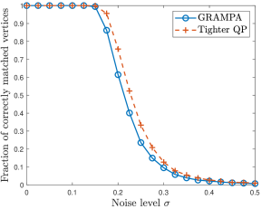
Figure 2: Fraction of correctly matched pairs of vertices by GRAMPA and the tighter QP (72) (both followed by linear assignment rounding) on Erdős-Rényi graphs with 1000 vertices and edge density 0.5, averaged over 10 repetitions.

6.1 Structure of solutions to QP relaxations

Before proving Theorem 6.1, we first provide an overview of the structure of solutions to the QP relaxations (11), (72) and (71). Using the Karush–Kuhn–Tucker (KKT) conditions, the solution of (72) can be expressed as

$$X^{\mathsf{c}}=\sum_{i,j}\frac{\langle v_{i},\mu\rangle\langle w_{j},\mathbf{1}\rangle}{(\lambda_{i}-\mu_{j})^{2}+\eta^{2}}v_{i}w_{j}^{\top},$$ (77)

where $\mu\in{\mathbb{R}}^{n}$ is the dual variable corresponding to the row sum constraints, chosen so that $X^{\mathsf{c}}$ is feasible. Since

$$X^{\mathsf{c}}\mathbf{1}=\sum_{i,j}\frac{\langle w_{j},\mathbf{1}\rangle^{2}}{(\lambda_{i}-\mu_{j})^{2}+\eta^{2}}v_{i}v_{i}^{\top}\mu=\left\{\sum_{i}\tau_{i}v_{i}v_{i}^{\top}\right\}\mu,$$

where

$$\tau_{i}\triangleq\sum_{j}\frac{\langle w_{j},\mathbf{1}\rangle^{2}}{(\lambda_{i}-\mu_{j})^{2}+\eta^{2}}.$$ (78)

Solving $X^{\mathsf{c}}\mathbf{1}=\mathbf{1}$ yields

$$\mu=\sum_{i}\frac{\langle v_{i},\mathbf{1}\rangle}{\tau_{i}}v_{i},$$ (79)

so we obtain

$$X^{\mathsf{c}}=\sum_{i,j}\frac{1}{(\lambda_{i}-\mu_{j})^{2}+\eta^{2}}\frac{1}{\tau_{i}}v_{i}v_{i}^{\top}\mathbf{J}w_{j}w_{j}^{\top}.$$ (80)

Let us provide some heuristics regarding the solution $X^{\mathsf{c}}$. As before we can express $\tau_{i}$ via resolvents as follows:

$$\tau_{i}= ~{}\frac{1}{\eta}\operatorname{Im}\sum_{j}\frac{\langle w_{j},\mathbf{1}\rangle^{2}}{\mu_{j}-(\lambda_{i}+\mathbf{i}\eta)}=\frac{1}{\eta}\mathbf{1}^{\top}\bigg{[}\operatorname{Im}\sum_{j}\frac{1}{\mu_{j}-(\lambda_{i}+\mathbf{i}\eta)}w_{j}w_{j}^{\top}\bigg{]}\mathbf{1}$$

$$= ~{}\frac{1}{\eta}\operatorname{Im}[\mathbf{1}^{\top}R_{B}(\lambda_{i}+\mathbf{i}\eta)\mathbf{1}].$$ (81)

Invoking the resolvent bound (36), we expect $\tau_{i}\approx\frac{n}{\eta}\operatorname{Im}[m_{0}(\lambda_{i}+\mathbf{i}\eta)]$, where, by properties of the Stieltjes transform (cf. Proposition 4.4), $\operatorname{Im}[m_{0}(\lambda_{i}+\mathbf{i}\eta)]\approx\operatorname{Im}[m_{0}(\lambda_{i})]=\pi\rho(\lambda_{i})$ as $\eta\to 0$. Thus we have the approximation

$$X^{\mathsf{c}}\approx\frac{1}{\pi n}\sum_{i,j}\frac{\eta}{(\lambda_{i}-\mu_{j})^{2}+\eta^{2}}\frac{1}{\rho(\lambda_{i})}v_{i}v_{i}^{\top}\mathbf{J}v_{j}w_{j}^{\top},$$

Compared with the unconstrained solution (3), apart from normalization, the only difference is the extra spectral weight $\frac{1}{\rho(\lambda_{i})}$ according to the inverse semicircle density. The effect is that eigenvalues near the edge are upweighted while eigenvalues in the bulk are downweighted, the rationale being that eigenvectors corresponding to the extreme eigenvalues are more robust to noise perturbation.

Remark 6.1 (Structure of the QP solutions).

Let us point out that solution of various QP relaxations, including (71), (72), and (11), are of the following common form:

$$X=\sum_{i,j}\frac{\eta}{(\lambda_{i}-\mu_{j})^{2}+\eta^{2}}v_{i}v_{i}^{\top}Sw_{j}w_{j}^{\top},$$ (82)

where $S$ is an $n\times n$ matrix that can depend on $A$ and $B$. Specifically, from the loosest to the tightest relaxations, we have:

• For (11) with the total sum constraint, $S=\alpha\mathbf{J}$, where the dual variable $\alpha>0$ is chosen for feasility. Since scaling by $\alpha$ does not effect the subsequent rounding step, this is equivalent to (3) that we analyze.

• For (72) with the row sum constraint, $S=\mu\mathbf{1}^{\top}$ is rank-one with $\mu$ given in (79).

• For (71) without the positivity constraint, $S=\mu\mathbf{1}^{\top}+\mathbf{1}\nu^{\top}$ is rank-two. Unfortunately, the dual variables and the spectral structure of the optimal solution turn out to be difficult to analyze.

• For (71) with the positivity constraint, $S=\mu\mathbf{1}^{\top}+\mathbf{1}\nu^{\top}+H$, where $H\geq 0$ is the dual variable certifying the positivity of the solution and satisfies complementary slackness.

6.2 Proof of Theorem 6.1

We now apply the resolvent technique to analyze the behavior of the constrained solution $X^{\mathsf{c}}$ and establish its diagonal dominance.

6.2.1 Resolvent representation of the solution

We start by giving a resolvent representation of $X^{\mathsf{c}}$ via a contour integral.

Lemma 6.2.

Consider symmetric matrices $A$ and $B$ with the spectral decompositions (2), and suppose that $\|A\|\leq 2.5$. Then the solution $X^{\mathsf{c}}$ of the program (72) admits the following representation

$$X^{\mathsf{c}}=\frac{1}{2\pi}\operatorname{Re}\oint_{\Gamma}F(z)R_{A}(z)\mathbf{J}R_{B}(z+\mathbf{i}\eta),$$ (83)

where $\Gamma$ is defined by (17) and

$$F(z)\triangleq\frac{2\mathbf{i}}{\mathbf{1}^{\top}R_{B}(z+\mathbf{i}\eta)\mathbf{1}-\mathbf{1}^{\top}R_{B}(z-\mathbf{i}\eta)\mathbf{1}}.$$ (84)

Proof.

By (81) we have $\tau_{i}^{-1}=\eta F(\lambda_{i})$. This leads to the following contour representation of $X^{\mathsf{c}}$ analogous to (16) for the unconstrained solution:

$$X^{\mathsf{c}}= ~{}\eta\sum_{i}F(\lambda_{i})v_{i}v_{i}^{\top}\mathbf{J}\left\{\sum_{j}\frac{1}{(\lambda_{i}-\mu_{j})^{2}+\eta^{2}}w_{j}w_{j}^{\top}\right\}$$

$$\overset{\rm(a)}{=} ~{}\operatorname{Im}\left[\sum_{i}F(\lambda_{i})v_{i}v_{i}^{\top}\mathbf{J}R_{B}(\lambda_{i}+\mathbf{i}\eta)\right]$$

$$\overset{\rm(b)}{=} ~{}\operatorname{Im}\left[\frac{1}{-2\pi\mathbf{i}}\oint_{\Gamma}F(z)R_{A}(z)\mathbf{J}R_{B}(z+\mathbf{i}\eta)\right]$$

$$= ~{}\frac{1}{2\pi}\operatorname{Re}\oint_{\Gamma}F(z)R_{A}(z)\mathbf{J}R_{B}(z+\mathbf{i}\eta),$$

where (a) follows from the Ward identity (Lemma 3.1); (b) follows from Cauchy integral formula and the analyticity of $F$ in the region enclosed by the contour $\Gamma$. ∎

6.2.2 Entrywise approximation

For some small constant $\varepsilon>0$, let $b,b^{\prime}$ be as defined in Theorem 4.5. Under the assumptions of Theorem 6.1, we have $c_{0}>b^{\prime}$ for $\varepsilon$ sufficiently small, so that Theorem 4.5 applies. Recall the notation $\delta_{1},\ldots,\delta_{4}$ defined in (45). For sufficiently small $\varepsilon>0$, we may also verify under the assumptions of Theorem 6.1 that $\delta_{i}=o(1)$ for each $i=1,2,3,4$, and

$$\frac{\delta_{1}\delta_{2}^{2}n}{\eta}\leq 1,\quad\frac{\delta_{2}^{2}\delta_{3}n}{\eta^{2}}\leq\frac{(\log n)^{\kappa}}{\sqrt{\eta}},\quad\text{ and }\quad\delta_{3}\leq\eta^{3}.$$ (85)

We also assume throughout the proof that the high-probability event $\|A\|\leq 2.5$ holds.

Thanks to (36), we can approximate $F(z)$ by

$$\widetilde{F}(z)=\frac{1}{n}\frac{2\mathbf{i}}{m_{0}(z+\mathbf{i}\eta)-m_{0}(z-\mathbf{i}\eta)}$$ (86)

and approximate $X^{\mathsf{c}}$ by

$$\widetilde{X}^{\mathsf{c}}= ~{}\frac{1}{2\pi}\operatorname{Re}\oint_{\Gamma}\widetilde{F}(z)R_{A}(z)\mathbf{J}R_{B}(z+\mathbf{i}\eta)$$ (87)

$$= ~{}\frac{-1}{\pi n}\operatorname{Im}\oint_{\Gamma}\frac{1}{m_{0}(z+\mathbf{i}\eta)-m_{0}(z-\mathbf{i}\eta)}R_{A}(z)\mathbf{J}R_{B}(z+\mathbf{i}\eta).$$ (88)

The following lemma makes the approximation of $X^{\mathsf{c}}$ precise in the entrywise sense:

Lemma 6.3.

Suppose (85) holds. On the high-probability event where Theorem 4.5 holds and also $\|A\|\leq 2.5$,

$$\|\widetilde{X}^{\mathsf{c}}-X^{\mathsf{c}}\|_{\ell_{\infty}}\lesssim\frac{\delta_{2}^{2}\delta_{3}}{\eta^{2}}\leq\frac{(\log n)^{\kappa}}{n\sqrt{\eta}},$$ (89)

where $\delta_{2},\delta_{3}$ are defined in (45).

Proof.

For notational convenience, put $G(z)=2\mathbf{i}/(nF(z))$ and $\widetilde{G}(z)=2\mathbf{i}/(n\widetilde{F}(z))$. Note that $|\operatorname{Im}(z)|\leq\eta/2$ for $z\in\Gamma$, and thus $\operatorname{Im}(z+\mathbf{i}\eta)$ and $\operatorname{Im}(z-\mathbf{i}\eta)$ have different signs. Therefore

$$|\widetilde{G}(z)|\geq|\operatorname{Im}\widetilde{G}(z)|=|\operatorname{Im}m_{0}(z+\mathbf{i}\eta)|+|\operatorname{Im}m_{0}(z-\mathbf{i}\eta)|\gtrsim\eta,$$

where the last step follows from (31). Furthermore, by (36), we have $\sup_{z\in\Gamma}|G(z)-\widetilde{G}(z)|\leq 2C\delta_{3}$. In view of (85), $\delta_{3}\ll\eta$. Hence we have $|G(z)|\gtrsim\eta$ and

$$\sup_{z\in\Gamma}|F(z)-\widetilde{F}(z)|\lesssim\frac{1}{n}\frac{\delta_{3}}{\eta^{2}}.$$

Finally, by (83) and (87), we have

$$|(X^{\mathsf{c}}-\widetilde{X}^{\mathsf{c}})_{k\ell}|\leq\oint_{\Gamma}dz|F(z)-\widetilde{F}(z)||e_{k}^{\top}R_{A}(z)\mathbf{1}||e_{\ell}^{\top}R_{B}(z+\mathbf{i}\eta)\mathbf{1}|.$$

By (35), for all $k,\ell$, $|e_{k}^{\top}R_{A}(z)\mathbf{1}|\lesssim\delta_{2}\sqrt{n}$ and $|e_{\ell}^{\top}R_{B}(z+\mathbf{i}\eta)\mathbf{1}|\lesssim\delta_{2}\sqrt{n}$. Combining the last two displays yields the desired claim. ∎

In view of the entrywise approximation, we may switch our attention to the approximate solution $\widetilde{X}^{\mathsf{c}}$ and establish its diagonal dominance, assuming without loss of generality $\pi_{*}$ is the identity permutation. The proof parallels the analysis in Section 5 so we focus on the differences. To make the scaling identical to the unconstrained case, define

$$Y\triangleq n\widetilde{X}^{\mathsf{c}}=\frac{1}{2\pi}\operatorname{Re}\oint_{\Gamma}f(z)R_{A}(z)\mathbf{J}R_{B}(z+\mathbf{i}\eta),$$ (90)

with

$$f(z)\triangleq\frac{2\mathbf{i}}{m_{0}(z+\mathbf{i}\eta)-m_{0}(z-\mathbf{i}\eta)}.$$

Compared with the unconstrained solution (16), the only difference is the weighting factor $f(z)$.

We aim to show that with probability at least $1-n^{-D}$, for any constant $D>0$, the following holds:

1. For off-diagonals, we have

   $$\max_{k\neq\ell}|Y_{k\ell}|\lesssim\left(\log n\right)^{\kappa}/\sqrt{\eta}.$$ (91)

2. For diagonal entries, we have

   $$\min_{k}\left|Y_{kk}-\frac{4(1-\sigma^{2})}{\pi\eta}\right|\lesssim\frac{r(n)}{\eta}+\frac{\sigma}{\eta^{2}}+\left(\log n\right)^{\kappa}\frac{1}{\sqrt{\eta}}.$$ (92)

In view of Lemma 6.3, this implies the desired (73) and (74). Finally, analogous to Corollary 2.2, under the assumption (75) with constants $c=1/(64C^{2})$ and $c^{\prime}=1/(2C)$, for all sufficiently large $n$,

$$\frac{4(1-\sigma^{2})}{\pi\eta}\geq\frac{7}{8\eta}>C\left(\frac{r(n)}{\eta}+\frac{\sigma}{\eta^{2}}+2(\log n)^{\kappa}\frac{1}{\sqrt{\eta}}\right),$$

implying the diagonal dominance in (76).

6.2.3 Off-diagonal entries

Let us first consider $Y_{12}$. Recall that for $z\in\Gamma$, we have $|\operatorname{Im}(z+\mathbf{i}\eta)|\gtrsim\eta$, $|\operatorname{Im}(z-\mathbf{i}\eta)|\gtrsim\eta$, and these imaginary parts have opposite signs. Then

$$|f(z)|\leq\frac{2}{|\operatorname{Im}[m_{0}(z+\mathbf{i}\eta)-m_{0}(z-\mathbf{i}\eta)]|}=\frac{2}{|\operatorname{Im}m_{0}(z+\mathbf{i}\eta)|+|\operatorname{Im}m_{0}(z-\mathbf{i}\eta)|}\lesssim\frac{1}{\eta},$$ (93)

where the last step applies (31). Analogous to (52), we get

$$2\pi Y_{12} =\operatorname{Re}\left(\oint_{\Gamma}f(z)\left[\mathbf{e}_{1}^{\top}R_{A}(z)\mathbf{1}\right]\left[\mathbf{e}_{2}^{\top}R_{B}(z+\mathbf{i}\eta)\mathbf{1}\right]dz\right)$$

$$=\operatorname{Re}\left(\alpha-a_{1}^{\top}g-b_{2}^{\top}h+a_{1}^{\top}Mb_{2}\right)+O\left(\frac{\delta_{1}\delta^{2}_{2}n}{\eta}\right),$$ (94)

where

$$\alpha\triangleq ~{}\oint_{\Gamma}f(z)m_{0}(z)m_{0}(z+\mathbf{i}\eta)dz,$$ (95)

$$g\triangleq ~{}\oint_{\Gamma}f(z)m_{0}(z)m_{0}(z+\mathbf{i}\eta)R_{A}^{(12)}(z)\mathbf{1}_{n-2}dz,$$ (96)

$$h\triangleq ~{}\oint_{\Gamma}f(z)m_{0}(z)m_{0}(z+\mathbf{i}\eta)R_{B}^{(12)}(z+\mathbf{i}\eta)\mathbf{1}_{n-2}dz,$$ (97)

$$M\triangleq ~{}\oint_{\Gamma}f(z)m_{0}(z)m_{0}(z+\mathbf{i}\eta)R_{A}^{(12)}(z)\mathbf{J}_{n-2}R_{B}^{(12)}(z+\mathbf{i}\eta)dz.$$ (98)

Here the constant $\operatorname{Re}\alpha$ is in fact equal to $2\pi$, which is consistent with the row-sum constraints. Indeed, opening up $m_{0}(z)$ and applying the Cauchy integral formula, we have

$$\operatorname{Re}\alpha= ~{}\operatorname{Re}\oint dz\frac{2\mathbf{i}}{m_{0}(z+\mathbf{i}\eta)-m_{0}(z-\mathbf{i}\eta)}m_{0}(z)m_{0}(z+\mathbf{i}\eta)$$

$$= ~{}\int\rho(x)dx\operatorname{Re}\oint dz\frac{1}{x-z}\frac{2\mathbf{i}~{}m_{0}(z+\mathbf{i}\eta)}{m_{0}(z+\mathbf{i}\eta)-m_{0}(z-\mathbf{i}\eta)}$$

$$= ~{}\int\rho(x)dx\operatorname{Re}\left[(-2\pi\mathbf{i})\frac{2\mathbf{i}~{}m_{0}(x+\mathbf{i}\eta)}{m_{0}(x+\mathbf{i}\eta)-m_{0}(x-\mathbf{i}\eta)}\right]$$

$$= ~{}2\pi\int\rho(x)dx\operatorname{Re}\left[\frac{2\,m_{0}(x+\mathbf{i}\eta)}{2\mathbf{i}\operatorname{Im}m_{0}(x+\mathbf{i}\eta)}\right]=2\pi\int\rho(x)dx=2\pi.$$ (99)

As in Section 5.2.2, to bound the linear and bilinear terms, we need to bound the $\ell_{\infty}$-norms and $\ell_{2}$-norms of $g,h$ and $M$. Clearly, by (93), the $\ell_{\infty}$-norms are at most an $O(1/\eta)$ factor of those obtained in (61) and (62), i.e., $\|g\|_{\infty}\lesssim\delta_{2}\sqrt{n}/\eta$ and $\|M\|_{\infty}\lesssim\delta_{2}^{2}n/\eta$. The $\ell_{2}$-norms need to be bounded more carefully. The following result is the counterpart of Lemma 5.3:

Lemma 6.4.

Assume the same setting of Lemma 5.3, and define $M$, $g$, and $h$ as in (96–98) with $R_{A}$, $R_{B}$ in place of $R_{A}^{(12)},R_{B}^{(12)}$. Then $\|M\|_{F}^{2}\lesssim n^{2}/\eta$, $\|g\|^{2}\lesssim n\log(1/\eta)$, and $\|h\|^{2}\lesssim n\log(1/\eta)$.

Proof.

We start with $\|M\|_{F}$, as the arguments for $\|g\|$ and $\|h\|$ are analogous and simpler. Recall the contour $\Gamma^{\prime}$ from Fig. 1. Proceeding as in the proof of Lemma 5.3, we have

$$~{}\frac{1}{n^{2}}\|M\|_{F}^{2}$$

$$= ~{}-\oint_{\Gamma}dz\oint_{\Gamma^{\prime}}dw\;m_{0}(z)m_{0}(z+\mathbf{i}\eta)m_{0}(w)m_{0}(w-\mathbf{i}\eta)f(z)f(w)\times$$

$$\hskip 72.26999pt\frac{n^{-1}\mathbf{1}^{\top}(R_{A}(z)-R_{A}(w))\mathbf{1}}{z-w}\frac{n^{-1}\mathbf{1}^{\top}(R_{B}(z+\mathbf{i}\eta)-R_{B}(w-\mathbf{i}\eta))\mathbf{1}}{z+\mathbf{i}\eta-(w-\mathbf{i}\eta)}$$

$$= ~{}-\underbrace{\oint_{\Gamma}dz\oint_{\Gamma^{\prime}}dw\,m_{0}(z)m_{0}(z+\mathbf{i}\eta)m_{0}(w)m_{0}(w-\mathbf{i}\eta)f(z)f(w)\frac{m_{0}(z)-m_{0}(w)}{z-w}\frac{m_{0}(z+\mathbf{i}\eta)-m_{0}(w-\mathbf{i}\eta)}{z+\mathbf{i}\eta-(w-\mathbf{i}\eta)}}_{\mathrm{(I)}}$$

$$~{}+\mathrm{(II)},$$

where $\mathrm{(II)}$ denotes the remainder term. Applying (36), (93), and the boundedness of $m_{0}$, the residual term is bounded as

$$|\mathrm{(II)}|\lesssim\delta_{3}\oint_{\Gamma}dz\oint_{\Gamma^{\prime}}dw|f(z)||f(w)|\frac{1}{|z-w|}\frac{1}{|z+\mathbf{i}\eta-(w-\mathbf{i}\eta)|}\lesssim\frac{\delta_{3}}{\eta^{4}}\lesssim\frac{1}{\eta}.$$ (100)

To control the leading term $\mathrm{(I)}$, let us define the auxiliary contours $\gamma$ with vertices $\pm(2+2\eta)\pm(\eta/2)\mathbf{i}$ and $\gamma^{\prime}$ with vertices $\pm(2+\eta)\pm(\eta/4)\mathbf{i}$. By first deforming $\Gamma^{\prime}$ to $\gamma^{\prime}$ for each fixed $z\in\Gamma$, then deforming $\Gamma$ to $\gamma$, and finally taking the complex modulus and applying $|m_{0}|\lesssim 1$, we get

$$|\mathrm{(I)}|\lesssim ~{}\oint_{\gamma}dz\oint_{\gamma^{\prime}}dw\,|f(z)||f(w)|\left|\frac{m_{0}(z)-m_{0}(w)}{z-w}\right|\left|\frac{m_{0}(z+\mathbf{i}\eta)-m_{0}(w-\mathbf{i}\eta)}{z+\mathbf{i}\eta-(w-\mathbf{i}\eta)}\right|.$$

The reason for performing these deformations is that for any $z\in\gamma\cup\gamma^{\prime}$, since $\operatorname{Re}z\in[-2-2\eta,2+2\eta]$, we have from (31) that $\operatorname{Im}m_{0}(z+\mathbf{i}\eta)\asymp\sqrt{\eta+\zeta(z)}$ and $-\operatorname{Im}m_{0}(z-\mathbf{i}\eta)\asymp\sqrt{\eta+\zeta(z)}$, where $\zeta(z)$ is as defined in Proposition 4.4. Then we obtain from (93) the improved bound $|f(z)|\lesssim 1/\sqrt{\eta+\zeta(z)}$, and hence

$$|\mathrm{(I)}|\lesssim\oint_{\gamma}dz\oint_{\gamma^{\prime}}dw\,\frac{1}{\sqrt{\eta+\zeta(z)}}\frac{1}{\sqrt{\eta+\zeta(w)}}\left|\frac{m_{0}(z)-m_{0}(w)}{z-w}\right|\left|\frac{m_{0}(z+\mathbf{i}\eta)-m_{0}(w-\mathbf{i}\eta)}{z+\mathbf{i}\eta-(w-\mathbf{i}\eta)}\right|.$$

To bound the above integral, for a small constant $c_{0}>0$, consider the two cases where $|z-w|\geq c_{0}$ and $|z-w|<c_{0}$. For the first case $|z-w|\geq c_{0}$, we simply apply $|m_{0}|\lesssim 1$ and $\sqrt{\eta+\kappa}\geq\sqrt{\eta}$ to get that

$$\oint\oint_{|z-w|\geq c_{0}}dz\,dw\,\frac{1}{\sqrt{\eta+\zeta(z)}}\frac{1}{\sqrt{\eta+\zeta(w)}}\left|\frac{m_{0}(z)-m_{0}(w)}{z-w}\right|\left|\frac{m_{0}(z+\mathbf{i}\eta)-m_{0}(w-\mathbf{i}\eta)}{z+\mathbf{i}\eta-(w-\mathbf{i}\eta)}\right|\lesssim\frac{1}{\eta}.$$ (101)

In the second case $|z-w|<c_{0}$, we claim that for $c_{0}$ sufficiently small, we have

$$|m_{0}(z)-m_{0}(w)| \lesssim\sqrt{\eta+\zeta(z)}+\sqrt{\eta+\zeta(w)},$$ (102)

$$|m_{0}(z+\mathbf{i}\eta)-m_{0}(w-\mathbf{i}\eta)| \lesssim\sqrt{\eta+\zeta(z)}+\sqrt{\eta+\zeta(w)}.$$ (103)

Indeed, if $\zeta(z)>c_{0}$, then (102) and (103) hold because $\sqrt{\eta+\zeta(z)}+\sqrt{\eta+\zeta(w)}\asymp 1$. If instead $\zeta(z)\leq c_{0}$, say, $\operatorname{Re}z\geq 2-c_{0}$, then from the explicit form (29) for $m_{0}(z)$ we get $1+m_{0}(z)=\frac{2-z+\sqrt{z^{2}-4}}{2}$ and hence

$$|1+m_{0}(z)|\lesssim|z-2|+\sqrt{|z-2||z+2|}\asymp\sqrt{|z-2|}\asymp\sqrt{\eta+\zeta(z)}.$$

Furthermore, since $\operatorname{Re}w\geq\operatorname{Re}z-|z-w|\geq 2-2c_{0}$, we also have $|1+m_{0}(w)|\lesssim\sqrt{\eta+\zeta(w)}$. Then (102) follows from the triangle inequality. The case of $\operatorname{Re}z\leq-2+c_{0}$, and the argument for (103), are analogous.

Having established (102) and (103), we apply

$$\frac{\left(\sqrt{\eta+\zeta(z)}+\sqrt{\eta+\zeta(w)}\right)^{2}}{\sqrt{\eta+\zeta(z)}\sqrt{\eta+\zeta(w)}} \lesssim\frac{\sqrt{\eta+\max(\zeta(z),\zeta(w))}}{\sqrt{\eta+\min(\zeta(z),\zeta(w))}}$$

$$\leq\frac{\sqrt{\eta+\min(\zeta(z),\zeta(w))}+\sqrt{|\zeta(z)-\zeta(w)|}}{\sqrt{\eta+\min(\zeta(z),\zeta(w))}}\leq 1+\frac{\sqrt{|z-w|}}{\sqrt{\eta}}$$

to get

$$\oint\oint_{|z-w|<c_{0}}dz\,dw\,\frac{1}{\sqrt{\eta+\zeta(z)}}\frac{1}{\sqrt{\eta+\zeta(w)}}\left|\frac{m_{0}(z)-m_{0}(w)}{z-w}\right|\left|\frac{m_{0}(z+\mathbf{i}\eta)-m_{0}(w-\mathbf{i}\eta)}{z+\mathbf{i}\eta-(w-\mathbf{i}\eta)}\right|$$

$$\lesssim\oint\oint_{|z-w|<c_{0}}dz\,dw\,\left(1+\frac{\sqrt{|z-w|}}{\sqrt{\eta}}\right)\frac{1}{|z-w||z+\mathbf{i}\eta-(w-\mathbf{i}\eta)|}.$$

Then divide this into the integrals where $|z-w|<\eta$ and $|z-w|\geq\eta$, applying

$$\oint\oint_{|z-w|<\eta}dz\,dw\,\frac{1}{|z-w||z+\mathbf{i}\eta-(w-\mathbf{i}\eta)|}\lesssim\oint\oint_{|z-w|<\eta}dz\,dw\,\frac{1}{\eta^{2}}\lesssim\frac{1}{\eta}$$

and

$$\oint\oint_{\eta\leq|z-w|<c_{0}}dz\,dw\,\frac{\sqrt{|z-w|}}{\sqrt{\eta}}\cdot\frac{1}{|z-w||z+\mathbf{i}\eta-(w-\mathbf{i}\eta)|}$$

$$\lesssim\frac{1}{\sqrt{\eta}}\oint\oint_{\eta\leq|z-w|<c_{0}}dz\,dw\,\frac{1}{|z-w|^{3/2}}\lesssim\frac{1}{\sqrt{\eta}}\frac{1}{\sqrt{\eta}}\lesssim\frac{1}{\eta}.$$ (104)

Combining with the first case (101), we get $|\mathrm{(I)}|\lesssim 1/\eta$. Finally, combining with (100), we get $\|M\|_{F}^{2}\lesssim n^{2}/\eta$ as desired.

Next we bound $\|g\|$. Proceeding as in the proof of Lemma 5.3 and following the same argument as above, we get

$$\frac{1}{n}\|g\|^{2} \lesssim\oint_{\gamma}dz\oint_{\gamma^{\prime}}dw\,|f(z)||f(w)|\frac{|m_{0}(z)-m_{0}(w)|}{|z-w|}+O\left(\frac{\delta_{3}}{\eta^{3}}\right)$$

$$\lesssim\oint_{\gamma}dz\oint_{\gamma^{\prime}}dw\,\frac{1}{\sqrt{\eta+\zeta(z)}}\frac{1}{\sqrt{\eta+\zeta(w)}}\frac{|m_{0}(z)-m_{0}(w)|}{|z-w|}+O\left(\frac{\delta_{3}}{\eta^{3}}\right).$$

For $|z-w|\geq c_{0}$, we have

$$\oint\oint_{|z-w|\geq c_{0}}dzdw\frac{1}{\sqrt{\eta+\zeta(z)}}\frac{1}{\sqrt{\eta+\zeta(w)}}\frac{|m_{0}(z)-m_{0}(w)|}{|z-w|}$$

$$\lesssim\left(\oint\frac{1}{\sqrt{\eta+\zeta(z)}}dz\right)\left(\oint\frac{1}{\sqrt{\eta+\zeta(w)}}dw\right)\lesssim 1.$$

For $|z-w|<c_{0}$, we apply $|m_{0}(z)-m_{0}(w)|\lesssim\sqrt{\eta+\zeta(z)}+\sqrt{\eta+\zeta(w)}$ as above, so that

$$\oint\oint_{|z-w|<c_{0}}dzdw\frac{1}{\sqrt{\eta+\zeta(z)}}\frac{1}{\sqrt{\eta+\zeta(w)}}\frac{|m_{0}(z)-m_{0}(w)|}{|z-w|}$$

$$\lesssim\oint dz\frac{1}{\sqrt{\eta+\zeta(z)}}\oint dw\frac{1}{|z-w|}+\oint dw\frac{1}{\sqrt{\eta+\zeta(w)}}\oint dz\frac{1}{|z-w|}$$

$$\lesssim\log(1/\eta)\cdot\left(\oint dz\frac{1}{\sqrt{\eta+\zeta(z)}}+\oint dw\frac{1}{\sqrt{\eta+\zeta(w)}}\right)\lesssim\log(1/\eta).$$

Combining the above yields $\|g\|^{2}\lesssim n\log(1/\eta)$. The argument for $\|h\|^{2}$ is the same as that for $\|g\|^{2}$. ∎

Finally, proceeding as in (55)–(56) and using the preceeding norm bounds, we obtain from (94):

$$|Y_{12}|\lesssim~{}1+\delta_{4}\sqrt{n\log\frac{1}{\eta}}+\frac{\delta_{4}^{2}n}{\sqrt{\eta}}+\frac{\delta_{1}\delta^{2}_{2}n}{\eta}\lesssim\frac{\delta_{4}^{2}n}{\sqrt{\eta}}=\left(\log n\right)^{\kappa}/\sqrt{\eta},$$

with probability at least $1-n^{-D}$, for any constant $D$. This implies the desired (91) by the union bound.

6.2.4 Diagonal entries

We now consider $Y_{11}$. Following the derivation from (66) to (67) and using Lemma 6.4 in place of Lemma 5.3, we obtain, with probability at least $1-n^{-D}$ for any constant $D$,

$$\left|Y_{11}-\frac{1-\sigma^{2}}{2\pi}\operatorname{Re}\frac{\operatorname{Tr}(M)}{n}\right|\lesssim\left(\log n\right)^{\kappa}\frac{1}{\sqrt{\eta}},$$ (105)

where

$$M\triangleq ~{}\oint_{\Gamma}f(z)m_{0}(z)m_{0}(z+\mathbf{i}\eta)R_{A}^{(1)}(z)\mathbf{J}R_{B}^{(1)}(z+\mathbf{i}\eta)dz.$$

The trace is computed by the following result, which parallels Lemma 5.4 and Lemma 5.5:

Lemma 6.5.

Suppose $\delta_{3}\leq\eta^{2}$. Assume the setting of Lemma 5.4. Define

$$M=\oint_{\Gamma}f(z)m_{0}(z)m_{0}(z+\mathbf{i}\eta)R_{A}(z)\mathbf{J}R_{B}(z+\mathbf{i}\eta)dz.$$

Then

$$\frac{1}{n}\operatorname{Tr}(M)=\frac{8+o_{\eta}(1)}{\eta}+O\left(\frac{\sigma+\delta_{3}}{\eta^{2}}\right).$$

Proof.

Analogous to (70), we have $\frac{1}{n}\operatorname{Tr}(M)=\mathrm{(I)}-\mathrm{(II)}$, where

$$\mathrm{(I)} =\frac{1}{\mathbf{i}\eta}\oint_{\Gamma}f(z)m_{0}(z)m_{0}(z+\mathbf{i}\eta)\frac{1}{n}\mathbf{1}^{\top}(R_{B}(z+\mathbf{i}\eta)-R_{A}(z))\mathbf{1}dz$$

$$\mathrm{(II)} =\frac{1}{\mathbf{i}\eta}\oint_{\Gamma}f(z)m_{0}(z)m_{0}(z+\mathbf{i}\eta)\frac{1}{n}\mathbf{1}^{\top}R_{B}(z+\mathbf{i}\eta)(A-B)R_{A}(z)\mathbf{1}\,dz.$$

To bound (II), consider two cases:

• For $z\in\Gamma$ with $|\operatorname{Im}z|=\eta/2$, by the Ward identity and (36), we have

  $$\left\|R_{A}(z)\mathbf{1}\right\|^{2}=\frac{2}{\eta}|\operatorname{Im}\mathbf{1}^{\top}R_{A}(z)\mathbf{1}|\lesssim\frac{n}{\eta}(|\operatorname{Im}m_{0}(z)|+O(\delta_{3})).$$

  and similarly,

  $$\left\|R_{B}(z+\mathbf{i}\eta)\mathbf{1}\right\|^{2}\lesssim\frac{n}{\eta}(|\operatorname{Im}m_{0}(z+\mathbf{i}\eta)|+O(\delta_{3})).$$

  Thus it holds that

  $$\left|\mathbf{1}^{\top}R_{B}(z+\mathbf{i}\eta)(A-B)R_{A}(z)\mathbf{1}\right|\lesssim\frac{n\sigma}{\eta}\left(\sqrt{|\operatorname{Im}m_{0}(z)\operatorname{Im}m_{0}(z+\mathbf{i}\eta)|}+\sqrt{\delta_{3}}\right).$$

  Using (31) and (93), we conclude that

  $$|f(z)|\sqrt{|\operatorname{Im}m_{0}(z)\operatorname{Im}m_{0}(z+\mathbf{i}\eta)|}\leq\frac{2\sqrt{|\operatorname{Im}m_{0}(z)\operatorname{Im}m_{0}(z+\mathbf{i}\eta)|}}{|\operatorname{Im}m_{0}(z+\mathbf{i}\eta)|+|\operatorname{Im}m_{0}(z-\mathbf{i}\eta)|}\asymp 1$$

  for all $z\in\Gamma$ with $|\operatorname{Im}z|=\eta/2$.

• For $z\in\Gamma$ with $\operatorname{Re}z=\pm 3$, since $\|A\|\leq 2.5$, $\left|\mathbf{1}^{\top}R_{B}(z+\mathbf{i}\eta)(A-B)R_{A}(z)\mathbf{1}\right|\lesssim n\sigma$.

Furthermore, by (93), $|f(z)|\lesssim\frac{1}{\eta}$ for all $z\in\Gamma$. Combining the above two cases yields

$$|\mathrm{(II)}|\lesssim\frac{\sigma}{\eta^{2}}\left(1+\frac{\sqrt{\delta_{3}}}{\eta}\right)+\frac{\sigma}{\eta}\asymp\frac{\sigma}{\eta^{2}},$$

since $\delta_{3}\leq\eta^{2}$ by the assumption.

For (I), applying (36) again and plugging the definition of $f(z)$ yields

$$\mathrm{(I)}=\frac{2}{\eta}\oint_{\Gamma}m_{0}(z)m_{0}(z+\mathbf{i}\eta)\frac{m_{0}(z+\mathbf{i}\eta)-m_{0}(z)}{m_{0}(z+\mathbf{i}\eta)-m_{0}(z-\mathbf{i}\eta)}dz+O\left(\frac{\delta_{3}}{\eta^{2}}\right).$$

We now apply an argument similar to that of Lemma 5.5: Note that

$$|m_{0}(z+\mathbf{i}\eta)-m_{0}(z-\mathbf{i}\eta)|\geq\operatorname{Im}(m_{0}(z+\mathbf{i}\eta)-m_{0}(z-\mathbf{i}\eta))\gtrsim\eta$$

by (31), so the integrand is bounded for fixed $\eta$. Then deforming $\Gamma$ to $\Gamma_{\epsilon}$ with vertices $\pm(2+\varepsilon)\pm\mathbf{i}\varepsilon$, taking $\varepsilon\to 0$ for fixed $\eta$, and applying the bounded convergence theorem, we have the equality

$$\oint_{\Gamma}m_{0}(z)m_{0}(z+\mathbf{i}\eta)\frac{m_{0}(z+\mathbf{i}\eta)-m_{0}(z)}{m_{0}(z+\mathbf{i}\eta)-m_{0}(z-\mathbf{i}\eta)}dz$$

$$=\int_{2}^{-2}m_{0}^{+}(x)m_{0}(x+\mathbf{i}\eta)\frac{m_{0}(x+\mathbf{i}\eta)-m_{0}^{+}(x)}{m_{0}(x+\mathbf{i}\eta)-m_{0}(x-\mathbf{i}\eta)}dx+\int_{-2}^{2}m_{0}^{-}(x)m_{0}(x+\mathbf{i}\eta)\frac{m_{0}(x+\mathbf{i}\eta)-m_{0}^{-}(x)}{m_{0}(x+\mathbf{i}\eta)-m_{0}(x-\mathbf{i}\eta)}dx.$$ (106)

We show that these integrands are uniformly bounded over small $\eta$: For any constant $\delta>0$ and for $|x|\leq 2-\delta$, we have the lower bound

$$|m_{0}(x+\mathbf{i}\eta)-m_{0}(x-\mathbf{i}\eta)|=2\operatorname{Im}m_{0}(x+\mathbf{i}\eta)\gtrsim\sqrt{\zeta(x)+\eta}\geq\sqrt{\delta}.$$ (107)

Then the above integrands are bounded by $C/\sqrt{\delta}$ for $|x|\leq 2-\delta$. For $|x|\in[2-\delta,2]$, let us apply

$$|m_{0}(x+\mathbf{i}\eta)-m_{0}^{+}(x)|\lesssim\sqrt{\zeta(x)+\eta}$$

as follows from (102) and taking the limit $w\in\mathbb{C}^{+}\to x$. We have also $|m_{0}^{+}(x)-m_{0}^{-}(x)|\asymp\sqrt{\zeta(x)}\lesssim\sqrt{\zeta(x)+\eta}$, so that

$$|m_{0}(x+\mathbf{i}\eta)-m_{0}^{-}(x)|\lesssim\sqrt{\zeta(x)+\eta}.$$

Combining these cases with the first inequality of (107), we see that the integrands of (106) are uniformly bounded for all small $\eta$.

Now apply the bounded convergence theorem and take the limit $\eta\to 0$, noting that $\lim_{\eta\to 0}m_{0}(x+\mathbf{i}\eta)=m_{0}^{+}(x)$ and $\lim_{\eta\to 0}m_{0}(x-\mathbf{i}\eta)=m_{0}^{-}(x)$. We get

$$\lim_{\eta\to 0}\oint_{\Gamma}m_{0}(z)m_{0}(z+\mathbf{i}\eta)\frac{m_{0}(z+\mathbf{i}\eta)-m_{0}(z)}{m_{0}(z+\mathbf{i}\eta)-m_{0}(z-\mathbf{i}\eta)}dz$$

$$=\int_{-2}^{2}m_{0}^{-}(x)m_{0}^{+}(x)\frac{m_{0}^{+}(x)-m_{0}^{-}(x)}{m_{0}^{+}(x)-m_{0}^{-}(x)}dx=\int_{-2}^{2}|m_{0}^{+}(x)|^{2}dx=4.$$

This gives $\mathrm{(I)}=(8+o_{\eta}(1))/\eta+O(\delta_{3}/\eta^{2})$. Combining with the bound for $\mathrm{(II)}$ yields the lemma. ∎

Finally, combining (105) with Lemma 6.5 and $\delta_{3}\ll\eta$ from (85), and applying a union bound yields the desired (92).

7 Proof of resolvent bounds

In this section, we prove Theorem 4.5. The entrywise bounds of part (a) are essentially the local semicircle law of [EKYY13b, Theorem 2.8], restricted to the simpler domain $\{z:\operatorname{dist}(z,[-2,2])\geq(\log n)^{-a}\}$ and with small modifications of the logarithmic factors. The bound in (b) follows from (a) using a straightforward Schur complement identity. The bound in (c) is more involved, and relies on the fluctuation averaging technique of [EKYY13b, Section 5]. We provide a proof of all three statements using the tools of [EKYY13b].

For each statement, it suffices to establish the claim with the stated probability for each individual point $z\in D$. The uniform statement over $z\in D$ then follows from a union bound over a sufficiently fine discretization of $D$ (of cardinality an arbitrarily large polynomial in $n$) and standard Lipschitz bounds for $m_{0}$ and $R_{jk}$ on the event of $\|A\|\leq 2.5$—we omit these details for brevity.

7.1 Notation and matrix identities

In this section, for $S\subset[n]$, denote by $A^{(S)}\in\mathbb{R}^{n\times n}$ the matrix $A$ with all elements in rows and columns belonging to $S$ replaced by 0. Denote

$$R^{(S)}(z)=(A^{(S)}-z\mathbf{I})^{-1}\in\mathbb{C}^{n\times n}.$$

Note that $R^{(S)}(z)$ is block-diagonal with respect to the block decomposition $\mathbb{C}^{n}=\mathbb{C}^{S}\oplus\mathbb{C}^{[n]\setminus S}$, with $S\times S$ block equal to $(-1/z)\mathbf{I}_{|S|}$ and $([n]\setminus S)\times([n]\setminus S)$ block equal to the resolvent of the corresponding minor of $A$. (We will typically only access elements of $R^{(S)}$ in this $([n]\setminus S)\times([n]\setminus S)$ block, in which case $R^{(S)}$ may be understood as the resolvent of the minor of $A$.)

For $i\in[n]$, we write as shorthand

$$iS=\{i\}\cup S,\qquad\sum_{k}^{(S)}=\sum_{k\in[n]\setminus S}.$$

We usually omit the spectral argument $z$ for brevity.

Lemma 7.1 (Schur complement identities).

For any $j\in[n]$,

$$\frac{1}{R_{jj}}=a_{jj}-z-\sum_{k,\ell}^{(j)}a_{jk}R_{k\ell}^{(j)}a_{\ell j}.$$ (108)

For any $j\neq k\in[n]$,

$$R_{jk} =-R_{jj}\sum_{\ell}^{(j)}a_{j\ell}R^{(j)}_{\ell k}=R_{jj}R_{kk}^{(j)}\left(-a_{jk}+\sum_{\ell,m}^{(jk)}a_{j\ell}R_{\ell m}^{(jk)}a_{mk}\right),$$ (109)

$$\mathbf{e}_{k}^{\top}R =\mathbf{e}_{k}^{\top}R^{(j)}+\frac{R_{kj}}{R_{jj}}\cdot\mathbf{e}_{j}^{\top}R,$$ (110)

$$\frac{1}{R_{kk}} =\frac{1}{R_{kk}^{(j)}}-\frac{(R_{kj})^{2}}{R_{kk}^{(j)}R_{jj}R_{kk}}.$$ (111)

For any $j,k,\ell\in[n]$ with $j\notin\{k,\ell\}$,

$$R_{k\ell}=R_{k\ell}^{(j)}+\frac{R_{kj}R_{j\ell}}{R_{jj}}.$$ (112)

These identities hold also for any $S\subset[n]$ with $R$ replaced by $R^{(S)}$ and with $j,k,\ell\in[n]\setminus S$.

Proof.

For all but (110), see [EKYY13a, Lemma 4.5] and [EYY12, Lemma 4.2]. As for (110), it is equivalent to verify that (112) holds also for $\ell=j$, which simply follows from $R^{(j)}_{kj}=0$, due to the block diagonal structure of $R^{(j)}$. ∎

7.2 Entrywise bound

We say an event occurs w.h.p. if its probability is at least $1-e^{-c(\log n)^{1+\varepsilon}}$ for a universal constant $c>0$. Let us show that (33) and (34) hold for $z\in D$ w.h.p.

We start with (34). Note that the $j$th row $\{a_{jk}:k\in[n]\}$ is independent of $A^{(j)}$ and hence $R^{(j)}$. Applying (108), (22), and (25) conditional on $A^{(j)}$, w.h.p. for all $j$,

$$\left|\frac{1}{R_{jj}}+z+\frac{1}{n}\sum_{k}^{(j)}R_{kk}^{(j)}\right|=\left|a_{jj}-\sum_{k,\ell}^{(j)}a_{jk}R_{k\ell}^{(j)}a_{\ell j}+\frac{1}{n}\sum_{k}^{(j)}R_{kk}^{(j)}\right| \leq(\log n)^{2+2\varepsilon}\left(\frac{1}{\sqrt{d}}+\frac{2\|R^{(j)}\|_{\infty}}{\sqrt{d}}+\frac{\|R^{(j)}\|_{F}}{n}\right).$$

Note that $\|R^{(j)}\|_{\infty}\leq\|R^{(j)}\|$, $\|R^{(j)}\|_{F}\leq\sqrt{n}\|R^{(j)}\|$, and $d\leq n$. For $z\in D_{1}$ and any $S\subset[n]$, we have $\|R^{(S)}\|\leq 1/|\operatorname{Im}z|\leq(\log n)^{a}$. For $z\in D_{2}$, we have $\|R^{(S)}\|\leq 10$ on the event $\|A\|\leq 2.5$, which occurs w.h.p. by Lemma 4.1. Then in both cases, we get

$$\left|\frac{1}{R_{jj}}+z+\frac{1}{n}\sum_{k}^{(j)}R_{kk}^{(j)}\right|\lesssim\frac{(\log n)^{2+2\varepsilon+a}}{\sqrt{d}}.$$ (113)

Since $|z|\leq 10$, $|R_{kk}^{(j)}|\leq(\log n)^{a}$, and $d\gg(\log n)^{4+4\varepsilon}$, this implies $1/|R_{jj}|\lesssim(\log n)^{a}$. Let $m_{n}(z)=n^{-1}\operatorname{Tr}R(z)$ be the empirical Stieltjes transform. Then

$$\left|m_{n}-\frac{1}{n}\sum_{k}^{(j)}R_{kk}^{(j)}\right|=\left|\frac{1}{n}R_{jj}+\frac{1}{n}\sum_{k}^{(j)}(R_{kk}-R_{kk}^{(j)})\right|\overset{\eqref{eq:LOO}}{=}\left|\frac{1}{n}\sum_{k}\frac{R_{kj}^{2}}{R_{jj}}\right|=\frac{\|\mathbf{e}_{j}^{\top}R\|^{2}}{n|R_{jj}|}\leq\frac{\|R\|^{2}}{n|R_{jj}|}\lesssim\frac{(\log n)^{3a}}{n}.$$

Using $d\leq n$ and combining with (113), w.h.p. for all $j$,

$$\left|\frac{1}{R_{jj}}+z+m_{n}\right|\lesssim\frac{(\log n)^{2+2\varepsilon+a}}{\sqrt{d}}.$$ (114)

Then by the triangle inequality, also w.h.p. for all $j\neq k$,

$$\left|\frac{1}{R_{jj}}-\frac{1}{R_{kk}}\right|\lesssim\frac{(\log n)^{2+2\varepsilon+a}}{\sqrt{d}},$$

so

$$\left|\frac{m_{n}}{R_{jj}}-1\right|=\left|n^{-1}\sum_{k}\frac{R_{kk}-R_{jj}}{R_{jj}}\right|\leq\max_{k}\left|\frac{R_{kk}-R_{jj}}{R_{jj}}\right|=\max_{k}|R_{kk}|\left|\frac{1}{R_{jj}}-\frac{1}{R_{kk}}\right|\lesssim\frac{(\log n)^{2+2\varepsilon+2a}}{\sqrt{d}}.$$

For $d\gg(\log n)^{4+4\varepsilon+4a}$, this implies $\frac{3}{2}|R_{jj}|\geq|m_{n}|\geq|R_{jj}|/2$ w.h.p. for all $j$. Then also

$$\left|\frac{1}{R_{jj}}-\frac{1}{m_{n}}\right|=\frac{|R_{jj}-m_{n}|}{|R_{jj}||m_{n}|}\leq\max_{k}\frac{|R_{jj}-R_{kk}|}{|R_{jj}||m_{n}|}\leq\max_{k}\frac{2|R_{jj}-R_{kk}|}{|R_{jj}||R_{kk}|}=2\max_{k}\left|\frac{1}{R_{jj}}-\frac{1}{R_{kk}}\right|,$$

so

$$\left|\frac{1}{R_{jj}}-\frac{1}{m_{n}}\right|\lesssim\frac{(\log n)^{2+2\varepsilon+a}}{\sqrt{d}}.$$ (115)

Combining with (114), w.h.p. we have

$$\frac{1}{m_{n}}+z+m_{n}=r_{n},\qquad|r_{n}|\lesssim\frac{(\log n)^{2+2\varepsilon+a}}{\sqrt{d}}\ll(\log n)^{-a}.$$

Solving for $m_{n}$ yields

$$m_{n}\in\frac{-z+r_{n}\pm\sqrt{z^{2}-4-2zr_{n}+r_{n}^{2}}}{2}$$

where the right side denotes the two complex square-roots. Note that $|z^{2}-4|=|z-2|\cdot|z+2|\gtrsim(\log n)^{-a}|z|$ and $|z|\geq(\log n)^{-a}$ for all $z\in D$. Then, as $(\log n)^{-a}\gg|r_{n}|$, we have $|z^{2}-4|\gg|zr_{n}|\gg|r_{n}|^{2}$. Letting $m_{0}$ be the Stieltjes transform of the semicircle law, and letting $\widetilde{m}_{0}=1/m_{0}$ be the other root of the quadratic equation (30), we obtain by a Taylor expansion of the square-root that

$$\min(|m_{n}-m_{0}|,|m_{n}-\widetilde{m}_{0}|)\lesssim|r_{n}|\left(1+\frac{|z|}{\sqrt{|z^{2}-4|}}\right)\lesssim\frac{|r_{n}|}{\sqrt{\zeta(z)+|\operatorname{Im}z|}},$$ (116)

where $\zeta(z)$ is as defined in Proposition 4.4.

To argue that this bound holds for $|m_{n}-m_{0}|$ rather than $|m_{n}-\widetilde{m}_{0}|$, consider first $z\in D_{1}$ with $\operatorname{Im}z>0$. In this case $m_{n}\in{\mathbb{C}}_{+}$ and $\widetilde{m}_{0}\in{\mathbb{C}}_{-}$. Furthermore, note that (31) implies $\operatorname{Im}m_{0}(z)\geq(\operatorname{Im}z)/\sqrt{\zeta(z)+\operatorname{Im}z}$, and hence $\operatorname{Im}\widetilde{m}_{0}=-(\operatorname{Im}m_{0})/|m_{0}|^{2}\leq-c(\log n)^{-a}/\sqrt{\zeta(z)+\operatorname{Im}z}$. Since $\operatorname{Im}m_{n}>0$ and $|r_{n}|\ll(\log n)^{-a}$, (116) must hold for $|m_{n}-m_{0}|$ rather than $|m_{n}-\widetilde{m}_{0}|$. The same argument applies for $z\in D_{1}$ with $\operatorname{Im}z<0$. For $z\in D_{2}$, we have $||m_{0}(z)|-1|\geq c$ and hence $|m_{0}(z)-\widetilde{m}_{0}(z)|>c$ for a constant $c>0$. Consider the point $z^{\prime}\in D_{1}\cap D_{2}$ with $\operatorname{Re}z^{\prime}=\operatorname{Re}z$ and $\operatorname{Im}z^{\prime}=(\log n)^{-a}$. Note that for all $z\in D_{2}$, $|\frac{d}{dz}m_{0}(z)|\lesssim 1$ and, on the event $\|A\|\leq 2.5$, $|\frac{d}{dz}m_{n}(z)|\lesssim 1$ also. Thus $|m_{0}(z)-m_{0}(z^{\prime})|\leq C(\log n)^{-a}$ and $|m_{n}(z)-m_{n}(z^{\prime})|\leq C(\log n)^{-a}$. Since we have already shown that (116) holds for $|m_{n}(z^{\prime})-m_{0}(z^{\prime})|$ in the previous case, this implies also that (116) must hold for $|m_{n}-m_{0}|$ rather than for $|m_{n}-\widetilde{m}_{0}|$.

Applying $|\operatorname{Im}z|\geq(\log n)^{-a}$, (116) yields w.h.p.

$$|m_{n}-m_{0}|\lesssim(\log n)^{a/2}|r_{n}|\lesssim\frac{(\log n)^{2+2\varepsilon+3a/2}}{\sqrt{d}}.$$ (117)

Recalling (115), $|R_{jj}|\leq(\log n)^{a}$ and $|m_{n}|\leq\frac{3}{2}|R_{jj}|$, we get

$$|R_{jj}-m_{n}|\lesssim|R_{jj}||m_{n}|\cdot\frac{(\log n)^{2+2\varepsilon+a}}{\sqrt{d}}\lesssim\frac{(\log n)^{2+2\varepsilon+3a}}{\sqrt{d}}.$$ (118)

Combining the last two displayed equations gives the weak estimate

$$|R_{jj}-m_{0}|\lesssim\frac{(\log n)^{2+2\varepsilon+3a}}{\sqrt{d}}.$$

Since $d\gtrsim(\log n)^{4+4\varepsilon+6a}$ by assumption, this and $|m_{0}(z)|\asymp 1$ imply $|R_{jj}|\lesssim 1$ w.h.p. Then applying the last display and (117) to the first inequality of (118) yields the desired estimate

$$|R_{jj}-m_{0}|\leq|R_{jj}-m_{n}|+|m_{n}-m_{0}|\lesssim\frac{(\log n)^{2+2\varepsilon+3a/2}}{\sqrt{d}}.$$

To show (33) for the off-diagonals, we now apply (109), (22), (26) conditional on $R^{(jk)}$, $|R_{jj}|\lesssim 1$, $|R_{kk}^{(j)}|\lesssim 1$, $\|R^{(jk)}\|_{\infty}\leq(\log n)^{a}$, $\|R^{(jk)}\|_{F}\leq\sqrt{n}(\log n)^{a}$, and $d\leq n$ to get w.h.p.

$$|R_{jk}| =|R_{jj}||R_{kk}^{(j)}|\left|-a_{jk}+\sum_{\ell,m}^{(jk)}a_{j\ell}R_{\ell m}^{(jk)}a_{mk}\right|$$

$$\lesssim(\log n)^{2+2\varepsilon}\left(\frac{1}{\sqrt{d}}+\frac{2\|R^{(jk)}\|_{\infty}}{\sqrt{d}}+\frac{\|R^{(jk)}\|_{F}}{n}\right)\lesssim\frac{(\log n)^{2+2\varepsilon+a}}{\sqrt{d}}.$$

7.3 Row sum bound

We now show that (35) holds for $z\in D$ w.h.p. Set

$$\mathcal{Z}_{i}\triangleq\sum_{j,k}^{(i)}a_{ik}R_{kj}^{(i)}=\sum_{k}^{(i)}a_{ik}\left(\mathbf{e}_{k}^{\top}R^{(i)}\mathbf{1}\right)$$ (119)

where the last equality holds because $R^{(i)}_{ki}=0$ for $k\neq i$. Applying (109),

$$\mathbf{e}_{i}^{\top}R\mathbf{1}=\sum_{j}R_{ij}=R_{ii}-R_{ii}\mathcal{Z}_{i}.$$

Then applying (34), w.h.p. for every $i\in[n]$,

$$\left|\mathbf{e}_{i}^{\top}R\mathbf{1}\right|\lesssim 1+|\mathcal{Z}_{i}|.$$ (120)

Applying (23) conditional on $A^{(i)}$, w.h.p. for every $i\in[n]$,

$$|\mathcal{Z}_{i}|\leq(\log n)^{1+\varepsilon}\left(\frac{\max_{k\neq i}|\mathbf{e}_{k}^{\top}R^{(i)}\mathbf{1}|}{\sqrt{d}}+\sqrt{\frac{\sum_{k}^{(i)}|\mathbf{e}_{k}^{\top}R^{(i)}\mathbf{1}|^{2}}{n}}\right).$$ (121)

For the second term above, we apply $\|R^{(i)}\|\leq(\log n)^{a}$ w.h.p. to get

$$\sum_{k}^{(i)}\left|\mathbf{e}_{k}^{\top}R^{(i)}\mathbf{1}\right|^{2}\leq\mathbf{1}^{\top}\overline{R^{(i)}}R^{(i)}\mathbf{1}\leq(\log n)^{2a}n.$$ (122)

For the first term, we apply (110), (33), and (34) to get, w.h.p. for all $k\neq i$,

$$\left|\mathbf{e}_{k}^{\top}R^{(i)}\mathbf{1}\right|=\left|\mathbf{e}_{k}^{\top}R\mathbf{1}-\frac{R_{ki}}{R_{ii}}\cdot\mathbf{e}_{i}^{\top}R\mathbf{1}\right|\leq\left|\mathbf{e}_{k}^{\top}R\mathbf{1}\right|+\frac{C(\log n)^{2+2\varepsilon+a}}{\sqrt{d}}\left|\mathbf{e}_{i}^{\top}R\mathbf{1}\right|.$$ (123)

Applying $d\gg(\log n)^{4+4\varepsilon+2a}$ and substituting (122) and (123) into (121) and then into (120), we get that

$$\left|\mathbf{e}_{i}^{\top}R\mathbf{1}\right|\lesssim 1+(\log n)^{1+\varepsilon}\left(\frac{\max_{k}|\mathbf{e}_{k}^{\top}R\mathbf{1}|}{\sqrt{d}}+(\log n)^{a}\right)$$ (124)

Taking the maximum over $i$ and rearranging yields (35).

7.4 Total sum bound

Finally, we show that (36) holds with probability $1-e^{-c(\log n)(\log\log n)}$ for $z\in D$. As above, we set

$$\mathcal{Z}_{i}=\sum_{j,k}^{(i)}a_{ik}R_{kj}^{(i)}=\sum_{k}^{(i)}a_{ik}\left(\mathbf{e}_{k}^{\top}R^{(i)}\mathbf{1}\right).$$ (125)

Note that if we apply (122), (123), and (35) to (121), we obtain w.h.p. that for every $i\in[n]$,

$$|\mathcal{Z}_{i}|\leq(\log n)^{1+\varepsilon+a}.$$ (126)

The main step of the proof of (36) is to use the weak dependence of $\mathcal{Z}_{1},\ldots,\mathcal{Z}_{n}$ to obtain a bound on $n^{-1}\sum_{i}\mathcal{Z}_{i}$ that is better than $(\log n)^{1+\varepsilon+a}$. The idea is encapsulated by the following abstract lemma from [EKYY13b].

Lemma 7.2 (Fluctuation averaging).

Let $\Xi$ be an event defined by $A$, let $\mathcal{Z}_{1},\ldots,\mathcal{Z}_{n}$ be random variables which are functions of $A$, let $p$ be an ($n$-dependent) even integer, and let $x,y>0$ be deterministic positive quantities. Suppose there exist random variables $\mathcal{Z}_{i}^{[U]}$, indexed by $U\subseteq[n]$ and $i\in[n]\setminus U$, which satisfy $\mathcal{Z}_{i}^{[\emptyset]}=\mathcal{Z}_{i}$ as well as the following conditions:

1. Let $a_{i}$ denote the $i^{\text{th}}$ row of $A$. Then $\mathcal{Z}_{i}^{[U]}$ is independent of $\{a_{j}:j\in U\}$, and $\mathbb{E}_{i}\left[\mathcal{Z}_{i}^{[U]}\right]=0$ where $\mathbb{E}_{i}$ is the partial expectation over only $a_{i}$.

2. For any $U\subseteq S\subset[n]$ with $|S|\leq p$, and for any $i\notin S$, denote $u=|U|+1$ and

   $$\mathcal{Z}_{i}^{S,U}=\sum_{T:\,T\subseteq U}(-1)^{|T|}\mathcal{Z}_{i}^{[(S\setminus U)\cup T]}.$$ (127)

   Then for a constant $C>0$ and any integer $r\in[0,p]$,

   $$\mathbb{E}\left[\mathbbm{1}\{\Xi\}\left|\mathcal{Z}_{i}^{S,U}\right|^{r}\right]\leq\Big{(}y(Cxu)^{u}\Big{)}^{r}.$$

   Furthermore,

   $$x\leq 1/(p^{5}\log n).$$

3. Let $\mathcal{A}\subset\mathbb{R}^{n\times n}$ be the matrices satisfying $\Xi$, i.e., $\Xi=\{A\in\mathcal{A}\}$. Let $\mathcal{A}_{i}=\{B\in\mathbb{R}^{n\times n}:B^{(i)}=A^{(i)}\text{ for some }A\in\mathcal{A}\}$, and define the event $\Xi_{i}=\{A\in\mathcal{A}_{i}\}$. For a constant $C>0$ and any $U,S,i$ as above, $\mathbb{E}\left[\mathbbm{1}\{\Xi_{i}\}\left|\mathcal{Z}_{i}^{S,U}\right|^{2}\right]\leq n^{Cp}$.

4. For a constant $C>0$ and any $U\subseteq[n]$, $\mathbbm{1}\{\Xi\}\left|\mathcal{Z}_{i}^{[U]}\right|\leq yn^{C}$.

5. For a constant $\varepsilon>0$, $\mathbb{P}[\Xi]\geq 1-e^{-c(\log n)^{1+\varepsilon}p}$.

Then for constants $C^{\prime},n_{0}>0$ depending on $C,\varepsilon$ above, and for all $n\geq n_{0}$,

$$\mathbb{P}\left[\mathbbm{1}\{\Xi\}\left|n^{-1}\sum_{i}\mathcal{Z}_{i}\right|\geq p^{12}y(x^{2}+n^{-1})\right]\leq(C^{\prime}/p)^{p}.$$

Proof.

See [EKYY13b, Theorem 5.6]. (The theorem is stated for $1+\varepsilon=3/2$ in condition (v), but the proof holds for any $\varepsilon>0$.) ∎

The important condition encapsulating weak dependence above is (ii). Applying (ii) with $U=\emptyset$, the condition requires first that each $|\mathcal{Z}_{i}^{[S]}|$, and in particular each $|\mathcal{Z}_{i}|=|\mathcal{Z}_{i}^{[\emptyset]}|$, is of typical size $Cxy$. In the application of this lemma, for $S=U$ and $i\notin U$, we will define the variables $\mathcal{Z}_{i}^{[V]}$ for $\emptyset\subseteq V\subseteq U$ such that the quantity $\mathcal{Z}_{i}^{U,U}$ in (127) is the variable $\mathcal{Z}_{i}$ with its dependence on all $\{a_{j}:j\in U\}$ projected out by an inclusion-exclusion procedure. Then condition (ii) requires that $\mathcal{Z}_{i}$ depends weakly on $\{a_{j}:j\in U\}$, in the sense that $|\mathcal{Z}_{i}^{U,U}|$ is of typical size $x^{|U|+1}y\cdot(C(|U|+1))^{|U|+1}$, which is roughly smaller than $|\mathcal{Z}_{i}|$ by a factor of $x|U|$ for each element of $U$. Assuming $1/\sqrt{n}\ll x\ll p^{-12}$, the above then estimates the average $|n^{-1}\sum_{i}\mathcal{Z}_{i}|$ to be of the smaller order $p^{12}yx^{2}\ll xy$. We refer the reader to the discussion in [EKYY13b] for additional details.

We will check that the conditions of this lemma hold for $\mathcal{Z}_{i}$ as defined by (125), with the appropriate construction of variables $\mathcal{Z}_{i}^{[U]}$. To this end, we first extend (33), (34), and (35) to $R^{(S)}$ for $|S|\leq\log n$ in the following deterministic lemma:

Lemma 7.3.

Suppose (33), (34), and (35) hold with the constant $C\equiv C_{0}$ for a deterministic symmetric matrix $A$, some $z\in D$, and all $j,k\in[n]$. Then for all $S\subset[n]$ with $|S|\leq\log n$, and all $j\neq k\in[n]\setminus S$,

$$|R^{(S)}_{jj}(z)-m_{0}(z)| \leq\frac{2C_{0}(\log n)^{2+2\varepsilon+3a}}{\sqrt{d}},$$ (128)

$$|R^{(S)}_{jk}(z)| \leq\frac{2C_{0}(\log n)^{2+2\varepsilon+a}}{\sqrt{d}},$$ (129)

$$|\mathbf{e}_{j}^{\top}R^{(S)}(z)\mathbf{1}| \leq 2C_{0}(\log n)^{1+\varepsilon+a}.$$ (130)

Proof.

For integers $s\geq 0$, let

$$\Lambda_{s}^{d} =\max\Big{\{}|R_{jj}^{(S)}-m_{0}|:\;|S|=s,\;j\in[n]\setminus S\Big{\}},$$

$$\Lambda_{s}^{o} =\max\Big{\{}|R_{jk}^{(S)}|:\;|S|=s,\;j\neq k\in[n]\setminus S\Big{\}}.$$

When (33) and (34) hold, we have that $\Lambda_{s}^{d}\leq C_{0}(\log n)^{2+2\varepsilon+3a}/\sqrt{d}$ and $\Lambda_{s}^{o}\leq C_{0}(\log n)^{2+2\varepsilon+a}/\sqrt{d}$ for $s=0$. By (112), we have for each $s\geq 1$ and $*\in\{d,o\}$ that

$$\Lambda_{s+1}^{*}\leq\Lambda_{s}^{*}+\frac{(\Lambda_{s}^{o})^{2}}{|m_{0}|-\Lambda_{s}^{d}}.$$ (131)

Assume inductively that for some $s\leq\log n$,

$$\Lambda_{s}^{d}\leq\frac{C_{0}(\log n)^{2+2\varepsilon+3a}}{\sqrt{d}}\left(1+\frac{4C_{0}(\log n)^{2+2\varepsilon+a}}{|m_{0}|\sqrt{d}}\right)^{s},\;\Lambda_{s}^{o}\leq\frac{C_{0}(\log n)^{2+2\varepsilon+a}}{\sqrt{d}}\left(1+\frac{4C_{0}(\log n)^{2+2\varepsilon+a}}{|m_{0}|\sqrt{d}}\right)^{s}.$$ (132)

Applying $d\gg(\log n)^{6+4\varepsilon+2a}$, $|m_{0}|\geq c$, and $s\leq\log n$, this implies in particular that

$$\Lambda_{s}^{d}\leq\frac{2C_{0}(\log n)^{2+2\varepsilon+3a}}{\sqrt{d}},\qquad\Lambda_{s}^{o}\leq\frac{2C_{0}(\log n)^{2+2\varepsilon+a}}{\sqrt{d}}.$$

We then have $|m_{0}|-\Lambda_{s}^{d}\geq|m_{0}|/2$ for $d\gg(\log n)^{4+4\varepsilon+6a}$, so (131) yields

$$\Lambda_{s+1}^{*}\leq\max(\Lambda_{s}^{*},\Lambda_{s}^{o})\left(1+\frac{2\Lambda_{s}^{o}}{|m_{0}|}\right)\leq\max(\Lambda_{s}^{*},\Lambda_{s}^{o})\left(1+\frac{4C_{0}(\log n)^{2+2\varepsilon+a}}{|m_{0}|\sqrt{d}}\right).$$

Thus both bounds of (132) hold for $s+1$, completing the induction. This establishes (128) and (129).

To show (130), set

$$\Gamma_{s}=\max\{|\mathbf{e}_{j}^{\top}R^{(S)}\mathbf{1}|:\;|S|=s,\;j\notin S\}.$$

When (35) holds, $\Gamma_{0}\leq C_{0}(\log n)^{1+\varepsilon+a}$. Applying (110) and the bound $|m_{0}|-\Lambda_{s}^{d}\geq|m_{0}|/2$, we have

$$\Gamma_{s+1}\leq(1+2\Lambda_{s}^{o}/|m_{0}|)\Gamma_{s}\overset{(\ref{eq:offdiagRS})}{\leq}\left(1+\frac{4C_{0}(\log n)^{2+2\varepsilon+3a}}{|m_{0}|\sqrt{d}}\right)\Gamma_{s},$$

Thus $\Gamma_{s}\leq 2\Gamma_{0}$ for all $s\leq\log n$. ∎

Lemma 7.4.

Fix $z\in D$. Let $\mathcal{Z}_{i}$ be defined in (125). For $U\subset[n]$ not containing $i$, define

$$\mathcal{Z}_{i}^{[U]}=\sum_{j,k}^{(iU)}a_{ik}R_{kj}^{(iU)}=\sum_{k}^{(iU)}a_{ik}(\mathbf{e}_{k}^{\top}R^{(iU)}\mathbf{1}).$$

Let $\Xi$ be the event where

• (33), (34), and (35) all hold at $z$, for all distinct $j,k\in[n]$,

• $|a_{ij}|\leq 1$ for all $i,j\in[n]$, and

• $\|A\|\leq 2.5$.

Let $p\in[2,(\log n)-1]$ be an even integer, and set

$$x=\frac{(\log n)^{2+2\varepsilon+a}}{\sqrt{d}},\qquad y=C^{\prime}\sqrt{d}(\log n)^{-\varepsilon}$$

for a sufficiently large constant $C^{\prime}>0$. Then all of the conditions of Lemma 7.2 are satisfied.

Proof.

Condition (i) is clear by definition, as row $a_{i}$ of $A$ is independent of $R^{(iU)}$.

To check (ii), note first that the bound $x\leq 1/(p^{5}\log n)$ follows from $d\geq(\log n)^{16+4\varepsilon+2a}$. For $U\subseteq S$ and $i\notin S$ we write

$$\mathcal{Z}_{i}^{S,U} =\sum_{T:\;T\subseteq U}(-1)^{|T|}\mathcal{Z}_{i}^{[(S\setminus U)\cup T]}$$

$$=\sum_{T:\;T\subseteq U}(-1)^{|T|}\sum_{k}^{((iS\setminus U)\cup T)}a_{ik}(\mathbf{e}_{k}^{\top}R^{((iS\setminus U)\cup T)}\mathbf{1})$$

$$=\sum_{k\in U}a_{ik}\left(\sum_{T:\;T\subseteq U\setminus\{k\}}(-1)^{|T|}(\mathbf{e}_{k}^{\top}R^{((iS\setminus U)\cup T)}\mathbf{1})\right)+\sum_{k}^{(iS)}a_{ik}\left(\sum_{T:\;T\subseteq U}(-1)^{|T|}(\mathbf{e}_{k}^{\top}R^{((iS\setminus U)\cup T)}\mathbf{1})\right)$$

$$\triangleq\sum_{k\in U}a_{ik}\alpha_{k}+\sum_{k}^{(iS)}a_{ik}\beta_{k}.$$

We claim that deterministically on the event $\Xi$, there is a constant $C>0$ such that for any $W,V\subset[n]$ disjoint with $|W\cup V|\leq\log n$, and any $i\notin W\cup V$, we have

$$\left|\sum_{T:\;T\subseteq W}(-1)^{|T|}\left(\mathbf{e}_{i}^{\top}R^{(V\cup T)}\mathbf{1}\right)\right|\leq\widetilde{y}(Cxw)^{w},$$ (133)

where $w=|W|+1$, $x=(\log n)^{2+2\varepsilon+a}/\sqrt{d}$, and $\widetilde{y}=C\sqrt{d}(\log n)^{-1-\varepsilon}$. We will verify this claim at the end of the proof. Assuming this claim, we apply it above with $V=iS\setminus U$ and either $W=U$ or $W=U\setminus\{k\}$. Then setting $u=|U|+1\geq w$, we have on $\Xi$ that

$$|\alpha_{k}|\leq\widetilde{y}(Cxu)^{|U|},\qquad|\beta_{k}|\leq\widetilde{y}(Cxu)^{|U|+1}.$$ (134)

Let $r$ be any even integer with $r\leq p\leq(\log n)-1$. As $\alpha_{k},\beta_{k}$ are independent of row $a_{i}$ of $A$ by definition, we have for the partial expectation $\mathbb{E}_{i}$ over $a_{i}$ that

$$\mathbb{E}_{i}\left[\mathbbm{1}\{\Xi\}\left|\mathcal{Z}_{i}^{S,U}\right|^{r}\right]$$

$$=\mathbb{E}_{i}\left[\mathbbm{1}\{\Xi\}\left|\sum_{k\in U}a_{ik}\alpha_{k}+\sum_{k}^{(iS)}a_{ik}\beta_{k}\right|^{r}\right]$$

$$\leq\mathbbm{1}\{|\alpha_{k}|\leq\widetilde{y}(Cxu)^{|U|}\text{ and }|\beta_{k}|\leq\widetilde{y}(Cxu)^{|U|+1}\text{ for all }k\}\cdot\mathbb{E}_{i}\left[\left|\sum_{k\in U}a_{ik}\alpha_{k}+\sum_{k}^{(iS)}a_{ik}\beta_{k}\right|^{r}\right].$$

We apply (24) for the conditional expectation $\mathbb{E}_{i}$, with $v$ having entries $v_{k}=\alpha_{k}$ for $k\in U$, $v_{k}=\beta_{k}$ for $k\notin iS$, and $v_{k}=0$ otherwise. Recall that $w\leq|U|\leq|S|\leq\log n$. Since $Cxw\ll 1$ and $|U|(Cxw)^{2|U|}\ll(n-|U|)(Cxw)^{2|U|+2}$ by the definition of $x$ and $d\leq n$, the bounds (134) imply

$$\|v\|_{\infty}\leq\widetilde{y}(Cxu)^{|U|},\qquad\|v\|_{2}\leq\sqrt{2n}\cdot\widetilde{y}(Cxw)^{|U|+1}.$$

Then for a constant $C^{\prime}>0$, (24) gives

$$\mathbb{E}_{i}\left[\mathbbm{1}\{\Xi\}\left|\mathcal{Z}_{i}^{S,U}\right|^{r}\right]\leq(C^{\prime}r\widetilde{y}(Cxu)^{u})^{r}.$$

Then taking the full expectation and setting $y=C^{\prime}(\log n)\widetilde{y}\geq C^{\prime}r\widetilde{y}$ (since $r\leq p\leq\log n$) yields condition (ii).

For condition (iii), we have

$$\mathbb{E}\left[\mathbbm{1}\{\Xi_{i}\}\left|\mathcal{Z}_{i}^{S,U}\right|^{2}\right] \leq 2^{|U|}\sum_{T:\;T\subseteq U}\mathbb{E}[\mathbbm{1}\{\Xi_{i}\}|\mathcal{Z}_{i}^{[(S\setminus U)\cup T]}|^{2}]$$

$$=2^{|U|}\sum_{T:\;T\subseteq U}\sum_{k,k^{\prime}}^{((iS\setminus U)\cup T)}\mathbb{E}[a_{ik}a_{ik^{\prime}}]\mathbb{E}\left[\mathbbm{1}\{\Xi_{i}\}(\mathbf{e}_{k}^{\top}R^{((iS\setminus U)\cup T)}\mathbf{1})(\mathbf{e}_{k^{\prime}}^{\top}R^{((iS\setminus U)\cup T)}\mathbf{1})\right]$$

$$=2^{|U|}\sum_{T:\;T\subseteq U}\sum_{k}^{((iS\setminus U)\cup T)}\mathbb{E}[a_{ik}^{2}]\mathbb{E}\left[\mathbbm{1}\{\Xi_{i}\}\left|\mathbf{e}_{k}^{\top}R^{((iS\setminus U)\cup T)}\mathbf{1}\right|^{2}\right],$$

where the second line applies the independence of $a_{i}$ and $A^{(i)}$. Note that on $\Xi_{i}$, we have $\|A^{(i)}\|\leq 2.5$. Then applying $|U|\leq\log n$, the norm bound $\|R^{((iS\setminus U)\cup T)}\|\leq(\log n)^{a}$ on $\Xi_{i}$, and $\mathbb{E}[a_{ik}^{2}]\leq C^{2}/n$, we get (iii). For (iv), we apply the condition $|a_{ik}|\leq 1$ by definition of $\Xi$, together with the bound $\|R^{(iU)}\|\leq(\log n)^{a}$ on $\Xi$. Finally, (v) holds by the probability bound of $1-e^{-c(\log n)^{1+\varepsilon}}$ established for (33), (34), (35), (22), and in Lemma 4.1.

It remains to establish the claim (133). For $W=\emptyset$, this follows from (35). Assume then that $w\geq 1$, and write $W=\{j_{1},\ldots,j_{w-1}\}$ (in any order). For a function $f:\mathbb{R}^{n\times n}\to\mathbb{C}$ and any index $j\in[n]$, define $Q_{j}f:\mathbb{R}^{n\times n}\to\mathbb{C}$ by

$$(Q_{j}f)(A)=f(A)-f(A^{(j)}).$$

Note that if $f$ is in fact a function of $A^{(S)}$, i.e. $f(A)=f(A^{(S)})$ for every matrix $A\in\mathbb{R}^{n\times n}$, then $Q_{j}f(A)=f(A^{(S)})-f(A^{(jS)})$. Fix $i$ and $V$, and define $f(A)=\mathbf{e}_{i}^{\top}R^{(V)}\mathbf{1}$. This satisfies $f(A)=f(A^{(V)})$ for every $A$. Then by inclusion-exclusion, the quantity to be bounded is equivalently written as

$$\sum_{T:\;T\subseteq W}(-1)^{|T|}(\mathbf{e}_{i}^{\top}R^{(V\cup T)}\mathbf{1})=(Q_{j_{w-1}}\ldots Q_{j_{2}}Q_{j_{1}}f)(A).$$

We apply Schur complement identities to iteratively to expand $Q_{j_{w-1}}\ldots Q_{j_{1}}f$: First applying (110), we get

$$Q_{j_{1}}f(A)=\mathbf{e}_{i}^{\top}R^{(V)}\mathbf{1}-\mathbf{e}_{i}^{\top}R^{(j_{1}V)}\mathbf{1}=R_{ij_{1}}^{(V)}\cdot\frac{1}{R_{j_{1}j_{1}}^{(V)}}\cdot\mathbf{e}_{j_{1}}^{\top}R^{(V)}\mathbf{1}.$$

Then applying (110), (111), and (112) to the three factors on the right side above, and using the identity

$$xyz-\widetilde{x}\widetilde{y}\widetilde{z}=xy(z-\widetilde{z})+x(\widetilde{y}-y)\widetilde{z}+(\widetilde{x}-x)\widetilde{y}\widetilde{z},$$

we get

$$Q_{j_{2}}Q_{j_{1}}f(A) =R_{ij_{1}}^{(V)}\cdot\frac{1}{R_{j_{1}j_{1}}^{(V)}}\cdot\left(\frac{R_{j_{1}j_{2}}^{(V)}}{R_{j_{2}j_{2}}^{(V)}}\cdot\mathbf{e}_{j_{2}}^{\top}R^{(V)}\mathbf{1}\right)+R_{ij_{1}}^{(V)}\cdot\left(-\frac{\left(R_{j_{1}j_{2}}^{(V)}\right)^{2}}{R_{j_{1}j_{1}}^{(j_{2}V)}R_{j_{2}j_{2}}^{(V)}R_{j_{1}j_{1}}^{(V)}}\right)\cdot\mathbf{e}_{j_{1}}^{\top}R^{(j_{2}V)}\mathbf{1}$$

$$\hskip 72.26999pt+\frac{R_{ij_{2}}^{(V)}R_{j_{2}j_{1}}^{(V)}}{R_{j_{2}j_{2}}^{(V)}}\cdot\frac{1}{R_{j_{1}j_{1}}^{(j_{2}V)}}\cdot\mathbf{e}_{j_{1}}^{\top}R^{(j_{2}V)}\mathbf{1}.$$

Applying (112), (111), and (110) to each factor of each summand above, and repeating iteratively, an induction argument verifies the following claims for each $t\in\{1,\ldots,w-1\}$:

• $Q_{j_{t}}\ldots Q_{j_{1}}f(A)$ is a sum of at most $\prod_{s=1}^{t-1}4s$ summands (with the convention $\prod_{s=1}^{0}4s=1$), where

• Each summand is a product of at most $4t$ factors, where

• jach factor is one of the following three forms, for a set $S\subseteq V\cup W$: $R^{(S)}_{jk}$ for $j,k\notin S$ distinct, or $1/R^{(S)}_{jj}$ for $j\notin S$, or $\mathbf{e}_{j}^{\top}R^{(S)}\mathbf{1}$ for $j\notin S$. Furthermore,

• Each summand of $Q_{j_{t}}\ldots Q_{j_{1}}f(A)$ satisfies: (a) It has exactly one factor of the form $\mathbf{e}_{j}^{\top}R^{(S)}\mathbf{1}$. (b) The number of factors of the form $1/R_{jj}^{(S)}$ is less than or equal to the number of factors of the form $R_{jk}^{(S)}$ for $j\neq k$. (c) There are at least $t$ factors of the form $R^{(S)}_{jk}$ for $j\neq k$.

Finally, we apply this with $t=w-1$ and use the bound

$$\prod_{s=1}^{t-1}4s\leq(4w)^{w}.$$

By Lemma 7.3, since $|W\cup V|\leq\log n$, we have $|R_{jk}^{(S)}|\leq C(\log n)^{2+2\varepsilon+a}/\sqrt{d}$, $|R_{jj}^{(S)}|\geq|m_{0}|/2$, and $|\mathbf{e}_{j}^{\top}R^{(S)}\mathbf{1}|\leq C(\log n)^{1+\varepsilon+a}$ on the event $\Xi$. Thus we get

$$|Q_{j_{w-1}}\ldots Q_{j_{1}}f(A)|\leq(4w)^{w}\cdot\left(\frac{C(\log n)^{2+2\varepsilon+a}}{\sqrt{d}}\right)^{w-1}\cdot C(\log n)^{1+\varepsilon+a}\leq\widetilde{y}(C^{\prime}xw)^{w}$$

for $x=(\log n)^{2+2\varepsilon+a}/\sqrt{d}$ and $\widetilde{y}=C\sqrt{d}(\log n)^{-1-\varepsilon}$, as claimed. ∎

We now show (36) holds for $z\in D$ with probability $1-e^{-c(\log n)(\log\log n)}$. The diagonal bound (34) implies

$$|\operatorname{Tr}R-n\cdot m_{0}|\leq\frac{Cn(\log n)^{2+2\varepsilon+3a/2}}{\sqrt{d}}.$$ (135)

To bound the sum of off-diagonal elements of $R$, we apply (109) to write

$$\sum_{i\neq k}R_{ik}=-\sum_{i}R_{ii}\mathcal{Z}_{i}=-m_{0}\sum_{i}\mathcal{Z}_{i}-\sum_{i}(R_{ii}-m_{0})\mathcal{Z}_{i}.$$ (136)

Applying (34) and (126) yields

$$\sum_{i}|(R_{ii}-m_{0})\mathcal{Z}_{i}|\leq\frac{Cn(\log n)^{3+3\varepsilon+5a/2}}{\sqrt{d}}.$$ (137)

Then applying Lemma 7.2 with $x,y,\Xi$ as defined in Lemma 7.4 and with $p$ being the largest even integer less than $(\log n)-1$, we have

$$\mathbbm{1}\{\Xi\}\left|n^{-1}\sum_{i}\mathcal{Z}_{i}\right|\leq C(\log n)^{12}\cdot\sqrt{d}(\log n)^{-\varepsilon}\cdot(\log n)^{4+4\varepsilon+2a}/d\leq\frac{C(\log n)^{16+3\varepsilon+2a}}{\sqrt{d}}$$ (138)

with probability $1-e^{-c(\log n)(\log\log n)}$. Since $\mathbf{1}^{\top}R\mathbf{1}=\operatorname{Tr}R+\sum_{i\neq k}R_{ik}$, multiplying (138) by $n\cdot m_{0}$ and combining with (135)–(137) yields (36).

References

- [ABK15] Yonathan Aflalo, Alexander Bronstein, and Ron Kimmel. On convex relaxation of graph isomorphism. Proceedings of the National Academy of Sciences, 112(10):2942–2947, 2015.
- [BCL+18] Boaz Barak, Chi-Ning Chou, Zhixian Lei, Tselil Schramm, and Yueqi Sheng. (Nearly) efficient algorithms for the graph matching problem on correlated random graphs. arXiv preprint arXiv:1805.02349, 2018.
- [BCPP98] Rainer E Burkard, Eranda Cela, Panos M Pardalos, and Leonidas S Pitsoulis. The quadratic assignment problem. In Handbook of combinatorial optimization, pages 1713–1809. Springer, 1998.
- [Bia97] Philippe Biane. On the free convolution with a semi-circular distribution. Indiana University Mathematics Journal, pages 705–718, 1997.
- [DMWX18] Jian Ding, Zongming Ma, Yihong Wu, and Jiaming Xu. Efficient random graph matching via degree profiles. arxiv preprint arxiv:1811.07821, Nov 2018.
- [EKYY13a] László Erdős, Antti Knowles, Horng-Tzer Yau, and Jun Yin. The local semicircle law for a general class of random matrices. Electron. J. Probab, 18(59):1–58, 2013.
- [EKYY13b] László Erdős, Antti Knowles, Horng-Tzer Yau, and Jun Yin. Spectral statistics of Erdős–Rényi graphs I: local semicircle law. The Annals of Probability, 41(3B):2279–2375, 2013.
- [EYY12] László Erdős, Horng-Tzer Yau, and Jun Yin. Bulk universality for generalized Wigner matrices. Probability Theory and Related Fields, 154(1-2):341–407, 2012.
- [FMWX19] Zhou Fan, Cheng Mao, Yihong Wu, and Jiaming Xu. Spectral graph matching and regularized quadratic relaxations I: The Gaussian model. preprint, 2019.
- [HW71] D. L. Hanson and F. T. Wright. A bound on tail probabilities for quadratic forms in independent random variables. Ann. Math. Statist., 42:1079–1083, 1971.
- [MMS10] Konstantin Makarychev, Rajsekar Manokaran, and Maxim Sviridenko. Maximum quadratic assignment problem: Reduction from maximum label cover and LP-based approximation algorithm. Automata, Languages and Programming, pages 594–604, 2010.
- [PG11] Pedram Pedarsani and Matthias Grossglauser. On the privacy of anonymized networks. In ACM SIGKDD International Conference on Knowledge Discovery and Data Mining, pages 1235–1243, 2011.
- [PRW94] Panos M. Pardalos, Franz Rendl, and Henry Wolkowicz. The quadratic assignment problem: A survey and recent developments. In In Proceedings of the DIMACS Workshop on Quadratic Assignment Problems, volume 16 of DIMACS Series in Discrete Mathematics and Theoretical Computer Science, pages 1–42. American Mathematical Society, 1994.
- [RV13] Mark Rudelson and Roman Vershynin. Hanson-Wright inequality and sub-Gaussian concentration. Electron. Commun. Probab., 18:no. 82, 9, 2013.
- [ZBV08] Mikhail Zaslavskiy, Francis Bach, and Jean-Philippe Vert. A path following algorithm for the graph matching problem. IEEE Transactions on Pattern Analysis and Machine Intelligence, 31(12):2227–2242, 2008.