Spectral Graph Matching and Regularized Quadratic Relaxations I: The Gaussian Model

Abstract

Graph matching aims at finding the vertex correspondence between two unlabeled graphs that maximizes the total edge weight correlation. This amounts to solving a computationally intractable quadratic assignment problem. In this paper we propose a new spectral method, GRAph Matching by Pairwise eigen-Alignments (GRAMPA). Departing from prior spectral approaches that only compare top eigenvectors, or eigenvectors of the same order, GRAMPA first constructs a similarity matrix as a weighted sum of outer products between all pairs of eigenvectors of the two graphs, with weights given by a Cauchy kernel applied to the separation of the corresponding eigenvalues, then outputs a matching by a simple rounding procedure. The similarity matrix can also be interpreted as the solution to a regularized quadratic programming relaxation of the quadratic assignment problem.

For the Gaussian Wigner model in which two complete graphs on $n$ vertices have Gaussian edge weights with correlation coefficient $1-\sigma^{2}$, we show that GRAMPA exactly recovers the correct vertex correspondence with high probability when $\sigma=O(\frac{1}{\log n})$. This matches the state of the art of polynomial-time algorithms, and significantly improves over existing spectral methods which require $\sigma$ to be polynomially small in $n$. The superiority of GRAMPA is also demonstrated on a variety of synthetic and real datasets, in terms of both statistical accuracy and computational efficiency. Universality results, including similar guarantees for dense and sparse Erdős-Rényi graphs, are deferred to the companion paper [FMWX19].

1 Introduction

Given a pair of graphs, the problem of graph matching or network alignment refers to finding a bijection between the vertex sets so that the edge sets are maximally aligned [CFSV04, LR13, ESDS16]. This is a ubiquitous problem arising in a variety of applications, including network de-anonymization [NS08, NS09], pattern recognition [CFSV04, SS05], and computational biology [SXB08, KHGM16]. Finding the best matching between two graphs with adjacency matrices $A$ and $B$ may be formalized as the following combinatorial optimization problem over the set of permutations $\mathcal{S}_{n}$ on $\{1,\dots,n\}$:

$$\max_{\pi\in\mathcal{S}_{n}}\sum_{i,j=1}^{n}A_{ij}B_{\pi(i),\pi(j)}.$$ (1)

This is an instance of the notoriously difficult quadratic assignment problem (QAP) [PRW94, BCPP98], which is NP-hard to solve or to approximate within a growing factor [MMS10].

As the worst-case computational hardness of the QAP (1) may not be representative of typical graphs, various average-case models have been studied. For example, when the two graphs are isomorphic, the resulting graph isomorphism problem can be solved for Erdős-Rényi random graphs in linear time whenever information-theoretically possible [Bol82, CP08], but remains open to be solved in polynomial time for arbitrary graphs. In “noisy” settings where the graphs are not exactly isomorphic, there is a recent surge of interest in computer science, information theory, and statistics for studying random graph matching [YG13, LFP14, KHG15, FQRM⁺16, CK16, SGE17, CK17, DCKG18, BCL⁺18, CKMP18, DMWX18, MX19].

1.1 Random weighted graph matching

In this work, we study the following random weighted graph matching problem: Consider two weighted graphs with $n$ vertices, and a latent permutation $\pi^{*}$ on $\{1,\ldots,n\}$ such that vertex $i$ of the first graph corresponds to vertex $\pi^{*}(i)$ of the second. Denoting by $A$ and $B$ their (symmetric) weighted adjacency matrices, suppose that $\{(A_{ij},B_{\pi^{*}(i),\pi^{*}(j)}):1\leq i<j\leq n\}$ are independent pairs of positively correlated random variables. We wish to recover $\pi^{*}$ from $A$ and $B$.

Notable special cases of this model include the following:

• Erdős-Rényi graph model: $(A_{ij},B_{\pi^{*}(i),\pi^{*}(j)})$ is a pair of correlated Bernoulli random variables. Then $A$ and $B$ are Erdős-Rényi graphs with correlated edges. This model has been extensively studied in [PG11, LFP14, KL14, CK16, LS18, BCL⁺18, DCKG18, CKMP18, DMWX18].

• Gaussian Wigner model: $(A_{ij},B_{\pi^{*}(i),\pi^{*}(j)})$ is a pair of correlated Gaussian variables, for example, $B_{\pi^{*}(i),\pi^{*}(j)}=A_{ij}+\sigma Z_{ij}$ where $\sigma\geq 0$ and $A_{ij},Z_{ij}$ are independent standard Gaussians. Then $A$ and $B$ are complete graphs with correlated Gaussian edge weights. This model was proposed in [DMWX18, Section 2] as a prototype of random graph matching due to its simplicity, and certain results in the Gaussian model may be expected to carry over to dense Erdős-Rényi graphs.

Spectral methods have a long history in testing graph isomorphism [BGM82] and the graph matching problem [Ume88]. In this paper, we introduce a new spectral method for graph matching, for which we prove the following exact recovery guarantee in the Gaussian setting.

Theorem (Informal statement).

Under the Gaussian Wigner model, if $\sigma\leq c/\log n$ for a sufficiently small constant $c>0$, then a spectral algorithm recovers $\pi^{*}$ exactly with high probability.

We describe the method in Section 1.2 below. The algorithm may also be interpreted as a regularized convex relaxation of the QAP program (1), and we discuss this connection in Section 1.3. The performance guarantee matches the state of the art of polynomial-time algorithms, namely, the degree profile method proposed in [DMWX18], and exponentially improves the performance of existing spectral matching algorithms, which require $\sigma=\frac{1}{\mathrm{poly}(n)}$ as opposed to $\sigma=O(\frac{1}{\log n})$ for our proposal.

In a companion paper [FMWX19], we apply resolvent-based universality techniques to establish similar guarantees for our spectral method on non-Gaussian models, including dense and sparse Erdős-Rényi graphs. Our proofs here in the Gaussian model are more direct and transparent, using instead the rotational invariance of $A$ and $B$ and yielding slightly stronger guarantees.

A variant of our method may also be applied to match two bipartite random graphs, which we discuss in Section 2.3. This is an extension of the analysis in the non-bipartite setting, which is our primary focus.

1.2 A new spectral method

Write the spectral decompositions of the weighted adjacency matrices $A$ and $B$ as

$$A=\sum_{i=1}^{n}\lambda_{i}u_{i}u_{i}^{\top}\quad\text{ and }\quad B=\sum_{j=1}^{n}\mu_{j}v_{j}v_{j}^{\top}$$ (2)

where the eigenvalues are ordered such that

$$\lambda_{1}\geq\cdots\geq\lambda_{n}\quad\text{ and }\quad\mu_{1}\geq\cdots\geq\mu_{n}.$$

Algorithm 1 GRAMPA (GRAph Matching by Pairwise eigen-Alignments)

1:  Input: Weighted adjacency matrices $A$ and $B$ on $n$ vertices, a tuning parameter $\eta>0$.

2:  Output: A permutation $\widehat{\pi}\in\mathcal{S}_{n}$.

3:  Construct the similarity matrix

$$\widehat{X}=\sum_{i,j=1}^{n}w(\lambda_{i},\mu_{j})\cdot u_{i}u_{i}^{\top}\mathbf{J}v_{j}v_{j}^{\top}\in\mathbb{R}^{n\times n}$$ (3)

where $\mathbf{J}\in\mathbb{R}^{n\times n}$ denotes the all-one matrix and $w$ is the Cauchy kernel of bandwidth $\eta$:

$$w(x,y)=\frac{1}{(x-y)^{2}+\eta^{2}}.$$ (4)

4:  Output the permutation estimate $\widehat{\pi}$ by “rounding” $\widehat{X}$ to a permutation, for example, by solving the linear assignment problem (LAP)

$$\widehat{\pi}=\operatorname*{argmax}_{\pi\in\mathcal{S}_{n}}\sum_{i=1}^{n}\widehat{X}_{i,\pi(i)}.$$ (5)

Our new spectral method is given in Algorithm 1, which we refer to as graph matching by pairwise eigen-alignments (GRAMPA). Therein, the linear assignment problem (5) may be cast as a linear program (LP) over doubly stochastic matrices, i.e., the Birkhoff polytope (see (13) below), or solved efficiently using the Hungarian algorithm [Kuh55]. We advocate this rounding approach in practice, although our theoretical results apply equally to the simpler rounding procedure matching each $i$ to

$$\widehat{\pi}(i)=\operatorname*{argmax}_{j}\widehat{X}_{ij}.$$ (6)

We discuss the choice of the tuning parameter $\eta$ further in Section 4, and find in practice that the performance is not too sensitive to this choice.

Let us remark that Algorithm 1 exhibits the following two elementary but desirable properties.

• Unlike previous proposals, our spectral method is insensitive to the choices of signs for individual eigenvectors $u_{i}$ and $v_{j}$ in (2). More generally, it does not depend on the specific choice of eigenvectors if certain eigenvalues have multiplicity greater than one. This is because the similarity matrix (3) depends on the eigenvectors of $A$ and $B$ only through the projections onto their distinct eigenspaces.

• Let $\widehat{\pi}(A,B)$ denote the output of Algorithm 1 with inputs $A$ and $B$. For any fixed permutation $\pi$, denote by $B^{\pi}$ the matrix with entries $B^{\pi}_{ij}=B_{\pi(i),\pi(j)}$, and by $\pi\circ\widehat{\pi}$ the composition $(\pi\circ\widehat{\pi})(i)=\pi(\widehat{\pi}(i))$. Then we have the equivariance property

  $$\pi\circ\widehat{\pi}(A,B^{\pi})=\widehat{\pi}(A,B)$$ (7)

  and similarly for $A^{\pi}$. That is, the outputs given $(A,B^{\pi})$ and given $(A,B)$ represent the same matching of the underlying graphs. This may be verified from (3) as a consequence of the identity $\mathbf{J}=\mathbf{J}\Pi=\Pi\mathbf{J}$ for any permutation matrix $\Pi$.

To further motivate the construction (3), we note that Algorithm 1 follows the same general paradigm as several existing spectral methods for graph matching, which seek to recover $\pi^{*}$ by rounding a similarity matrix $\widehat{X}$ constructed to leverage correlations between eigenvectors of $A$ and $B$. These methods include:

• Low-rank methods that use a small number of eigenvectors of $A$ and $B$. The simplest such approach uses only the leading eigenvectors, taking as the similarity matrix

  $$\widehat{X}=u_{1}v_{1}^{\top}.$$ (8)

  Then $\widehat{\pi}$ which solves (5) orders the entries of $v_{1}$ in the order of $u_{1}$. Other rank-$1$ spectral methods and low-rank generalizations have also been proposed and studied in [FQRM⁺16, KG16].

• Full-rank methods that use all eigenvectors of $A$ and $B$. A notable example is the popular method of Umeyama [Ume88], which sets

  $$\widehat{X}=\sum_{i=1}^{n}s_{i}u_{i}v_{i}^{\top}$$ (9)

  where $s_{i}$ are signs in $\{-1,1\}$; see also the related approach of [XK01]. The motivation is that (9) is the solution to the orthogonal relaxation of the QAP (1), where the feasible set is relaxed to the set the orthogonal matrices [FBR87]. As the correct choice of signs in (9) may be difficult to determine in practice, [Ume88] suggests also an alternative construction

  $$\widehat{X}=\sum_{i=1}^{n}|u_{i}||v_{i}|^{\top}$$ (10)

  where $|u_{i}|$ denotes the entrywise absolute value of $u_{i}$.

Compared with these constructions, the proposed new spectral method has two important features that we elaborate below:

“All pairs matter.”

Departing from existing approaches, our proposal $\widehat{X}$ in (3) uses a combination of $u_{i}v_{j}^{\top}$ for all $n^{2}$ pairs $i,j\in\{1,\ldots,n\}$, rather than only $i=j$. This renders our method significantly more resilient to noise. Indeed, while all of the above methods can succeed in recovering $\pi^{*}$ in the noiseless case, methods based only on pairs $(u_{i},v_{i})$ with $i=j$ are brittle to noise if $u_{i}$ and $v_{i}$ quickly decorrelate as the amount of noise increases—this may happen when $\lambda_{i}$ is not separated from other eigenvalues by a large spectral gap. When this decorrelation occurs, $u_{i}$ becomes partially correlated with $v_{j}$ for neighboring indices $j$, and the construction (3) leverages these partial correlations in a weighted manner to provide a more robust estimate of $\pi^{*}$.

The eigenvector alignment is quantitatively understood in certain regimes for the Gaussian Wigner model $B=A+\sigma Z$ when $A,Z$ are GOE or GUE: It is known that $\mathbb{E}[\langle u_{i},v_{i}\rangle^{2}]=o(1)$ for the leading eigenvector $i=1$ as soon as $\sigma^{2}\gg n^{-1/3}$ [Cha14, Theorem 3.8], and for $i$ in the bulk of the Wigner semicircle spectrum as soon as $\sigma^{2}\gg n^{-1}$ [BY17, Ben17]. For $i$ in the bulk, and the noise regime $n^{-1+\varepsilon}\ll\sigma^{2}\ll n^{-\varepsilon}$, [Ben17, Theorem 1.3] further implies that $\langle u_{i},v_{j}\rangle$ is approximately Gaussian for each index $j$ sufficiently close to $i$, with zero mean and variance

$$\mathbb{E}[\langle u_{i},v_{j}\rangle^{2}]\approx\frac{\sigma^{2}/n}{(\lambda_{i}-\mu_{j})^{2}+C\sigma^{4}}.$$ (11)

Here, the value of $C\asymp 1$ depends on the Wigner semicircle density near $\lambda_{i}\approx\mu_{j}$. Thus, for this range of noise, the eigenvector $u_{i}$ of $A$ is most aligned with $O(n\sigma^{2})$ eigenvectors $v_{j}$ of $B$ for which $|\lambda_{i}-\mu_{j}|\lesssim\sigma^{2}$, and each such alignment is of typical size $\mathbb{E}[\langle u_{i},v_{j}\rangle^{2}]\asymp 1/(n\sigma^{2})\ll 1$. The signal for $\pi^{*}$ in our proposal (3) arises from a weighted average of these alignments. As a result, while existing spectral approaches are only robust up to a noise level $\sigma=\frac{1}{\mathrm{poly}(n)}$, our new spectral method is polynomially more robust and can tolerate $\sigma=O(\frac{1}{\log n})$.

Cauchy spectral weights.

The performance of the spectral method depends crucially on the choice of the weight function $w$ in (3). In fact, there are other methods that are also of the form (3) but do not work equally well. For example, if we choose $w(\lambda,\mu)=\lambda\mu$, then (3) simply reduces to $\widehat{X}=A\mathbf{J}B=ab^{\top}$, where $a=A\mathbf{1}$ and $b=B\mathbf{1}$ are the vectors of “degrees”. Rounding such a similarity matrix is equivalent to matching by sorting the degree of the vertices, which is known to fail when $\sigma=\Omega(n^{-1})$ due to the small spacing of the order statistics (cf. [DMWX18, Remark 1]).

The Cauchy spectral weight (4) is a particular instance of the more general form $w(\lambda,\mu)=K(\frac{|\lambda-\mu|}{\eta})$, where $K$ is a monotonically decreasing kernel function and $\eta$ is a bandwidth parameter. Such a choice upweights the eigenvector pairs whose eigenvalues are close and significantly penalizes those whose eigenvalues are separated more than $\eta$. The specific choice of the Cauchy kernel matches the form of $\mathbb{E}[\langle u_{i},v_{j}\rangle^{2}]$ in (11), and is in a sense optimal as explained by a heuristic signal-to-noise calculation in Appendix C. In addition, the Cauchy kernel has its genesis as a regularization term in the associated convex relaxation, which we explain next.

1.3 Connections to regularized quadratic programming

Our new spectral method is also rooted in optimization, as the similarity matrix $\widehat{X}$ in (3) corresponds to the solution to a convex relaxation of the QAP (1), regularized by an added ridge penalty.

Denote the set of permutation matrices in $\mathbb{R}^{n\times n}$ by $\mathfrak{S}_{n}$. Then (1) may be written in matrix notation as one of the three equivalent optimization problems

$$\max_{\Pi\in\mathfrak{S}_{n}}\,\langle A,\Pi B\Pi^{\top}\rangle\quad\Longleftrightarrow\quad\min_{\Pi\in\mathfrak{S}_{n}}\|A-\Pi B\Pi^{\top}\|_{F}^{2}\quad\Longleftrightarrow\quad\min_{\Pi\in\mathfrak{S}_{n}}\|A\Pi-\Pi B\|_{F}^{2}.$$ (12)

Note that the third objective $\|A\Pi-\Pi B\|_{F}^{2}$ above is a convex function in $\Pi$. Relaxing the set of permutations to its convex hull (the Birkhoff polytope of doubly stochastic matrices)

$$\mathcal{B}_{n}\triangleq\{X\in\mathbb{R}^{n\times n}:X\mathbf{1}=\mathbf{1},\,X^{\top}\mathbf{1}=\mathbf{1},\,X_{ij}\geq 0\text{ for all }i,j\},$$ (13)

we arrive at the quadratic programming (QP) relaxation

$$\min_{X\in\mathcal{B}_{n}}\|AX-XB\|_{F}^{2},$$ (14)

which was proposed in [ZBV08, ABK15], following an earlier LP relaxation using the $\ell_{1}$-objective proposed in [AD93]. Although this QP relaxation has achieved empirical success [ABK15, VCL⁺15, LFF⁺16, DML17], understanding its performance theoretically is a challenging task yet to be accomplished.

Our spectral method can be viewed as the solution of a regularized further relaxation of the doubly stochastic QP (14). Indeed, we show in Corollary 2.2 that the matrix $\widehat{X}$ in (3) is the minimizer of

$$\min_{X\in\mathbb{R}^{n\times n}}\frac{1}{2}\|AX-XB\|_{F}^{2}+\frac{\eta^{2}}{2}\|X\|_{F}^{2}-\mathbf{1}^{\top}X\mathbf{1}.$$ (15)

Equivalently, $\widehat{X}$ is a positive scalar multiple of the solution $\widetilde{X}$ to

$$\min_{X\in\mathbb{R}^{n\times n}} ~{}\|AX-XB\|_{F}^{2}+\eta^{2}\|X\|_{F}^{2}$$

s.t. $$~{}\mathbf{1}^{\top}X\mathbf{1}=n$$ (16)

which further relaxes (14) and adds a ridge penalty term $\eta^{2}\|X\|_{F}^{2}$. Note that $\widehat{X}$ and $\widetilde{X}$ are equivalent as far as the rounding step (5) or (6) is concerned. In contrast to (14), for which there is currently limited theoretical understanding, we are able to provide an exact recovery analysis for the rounded solutions to (15) and (16).

Note that the constraint in (16) is a significant relaxation of the double stochasticity (14). To make this further relaxed program work, the regularization term plays a key role. If $\eta$ were zero, the similarity matrix $\widehat{X}$ in (3) would involve the eigengap $|\lambda_{i}-\mu_{j}|$ in the denominator which can be polynomially small in $n$. Hence the regularization is crucial for reducing the variance of the estimate and making $\widehat{X}$ stable, a rationale reminiscent of the ridge regularization in high-dimensional linear regression. In a companion paper [FMWX19], we analyze a tighter relaxation than (16) which replaces $\mathbf{1}^{\top}X\mathbf{1}=n$ by the row-sum constraint $X\mathbf{1}=\mathbf{1}$, and there the ridge penalty is still indispensable for achieving exact recovery up to noise level $\sigma=O(1/\operatorname{polylog}(n))$.

Viewing $\widehat{X}$ as the minimizer of (15) provides not only an optimization perspective, but also an associated gradient descent algorithm to compute $\widehat{X}$. More precisely, starting from the initial point $X^{(0)}=0$ and fixing a step size $\gamma>0$, a straightforward computation verifies that gradient descent for optimizing (15) is given by the dynamics

$$X^{(t+1)}=X^{(t)}-\gamma\big{(}A^{2}X^{(t)}+X^{(t)}B^{2}-2AX^{(t)}B+\eta^{2}X^{(t)}-\mathbf{J}\big{)}.$$ (17)

Corollary 2.2 below shows that running gradient descent for $t=O\big{(}(\log n)^{3}\big{)}$ iterations suffices to produce a similarity matrix, which, upon rounding, exactly recovers $\pi^{*}$ with high probability, using $X^{(t)}$ in place of $\widehat{X}$ in (5). Each iteration involves several matrix multiplication operations with $A$ and $B$, which may be more efficient and parallelizable than performing spectral decompositions when the graphs are large and/or sparse.

1.4 Diagonal dominance of the similarity matrix

Equipped with this optimization point of view, we now explain the typical structure of solutions to the above quadratic programs including the spectral similarity matrix (3). It is well known that even the solution to the most stringent relaxation (14) is not the latent permutation matrix, which has been shown in [LFF⁺16] by proving that the KKT conditions cannot be fulfilled with high probability. In fact, a heuristic calculation explains why the solution to (14) is far from any permutation matrix: Let us consider the “population version” of (14), where the objective function is replaced by its expectation over the random instances $A$ and $B$. Consider $\pi^{*}=\mathsf{id}$ and the Gaussian Wigner model $B=A+\sigma Z$, where $A$ and $Z$ are independent GOE matrices with $N(0,\frac{1}{n})$ off-diagonal entries and $N(0,\frac{2}{n})$ diagonal entries. Then the expectation of the objective function is

$$\mathbb{E}\|AX-XB\|_{F}^{2} =\mathbb{E}\|AX\|_{F}^{2}+\mathbb{E}\|XB\|_{F}^{2}-2\mathbb{E}\langle AX,XA\rangle$$

$$=(2+\sigma^{2})\frac{n+1}{n}\|X\|_{F}^{2}-\frac{2}{n}\operatorname{Tr}(X)^{2}-\frac{2}{n}\langle X,X^{\top}\rangle.$$

Hence the population version of the quadratic program (14) is

$$\min_{X\in\mathcal{B}_{n}}(2+\sigma^{2})(n+1)\|X\|_{F}^{2}-2\operatorname{Tr}(X)^{2}-2\langle X,X^{\top}\rangle,$$ (18)

whose solution is

$$\overline{X}\triangleq\epsilon\mathbf{I}+(1-\epsilon)\mathbf{F},\qquad\epsilon=\frac{2}{2+(n+1)\sigma^{2}}\approx\frac{2}{n\sigma^{2}}.$$ (19)

This is a convex combination of the true permutation matrix and the center of the Birkhoff polytope $\mathbf{F}=\frac{1}{n}\mathbf{J}$. Therefore, the population solution $\overline{X}$ is in fact a very “flat” matrix, with each entry on the order of $\frac{1}{n}$, and is close to the center of the Birkhoff polytope and far from any of its vertices.

This calculation nevertheless provides us with important structural information about the solution to such a QP relaxation: $\overline{X}$ is diagonally dominant for small $\sigma$, with diagonals about $2/\sigma^{2}$ times the off-diagonals. Although the actual solution of the relaxed program (14) or (15) is not equal to the population solution $\overline{X}$ in expectation, it is reasonable to expect that it inherits the diagonal dominance property in the sense that $\widehat{X}_{i,\pi^{*}(i)}>\widehat{X}_{ij}$ for all $j\neq\pi^{*}(i)$, which enables rounding procedures such as (5) to succeed.

With this intuition in mind, let us revisit the regularized quadratic program (15) whose solution is the spectral similarity matrix (3). By a similar calculation, the solution to the population version of (15) is given by $\alpha\mathbf{I}+\beta\mathbf{J}$, with $\alpha=\frac{2n^{2}}{\left(n\left(\eta^{2}+\sigma^{2}\right)+\sigma^{2}\right)\left(n\left(\eta^{2}+\sigma^{2}+2\right)+\sigma^{2}\right)}\approx\frac{2}{\left(\eta^{2}+\sigma^{2}\right)\left(\eta^{2}+\sigma^{2}+2\right)}$ and $\beta=\frac{n}{n(\eta^{2}+\sigma^{2}+2)+\sigma^{2}}\approx\frac{1}{\eta^{2}+\sigma^{2}+2}$, which is diagonally dominant for small $\sigma$ and $\eta$. In turn, the basis of our theoretical guarantee is to establish the diagonal dominance of the actual solution $\widehat{X}$; see Fig. 1 for an empirical illustration.

Although the ridge penalty $\eta^{2}\|X\|_{F}^{2}$ guarantees the stability of the solution as discussed in Section 1.3, it may seem counterintuitive since it moves the solution closer to the center of the Birkhoff polytope and further away from the vertices (permutation matrices). In fact, several works in the literature [FJBd13, DML17] advocate adding a negative ridge penalty, in order to make the solution closer to a permutation at the price of potentially making the optimization non-convex. This consideration, however, is not necessary, as the ensuing rounding step can automatically map the solution to the correct permutation, even if they are far away in the Euclidean distance.

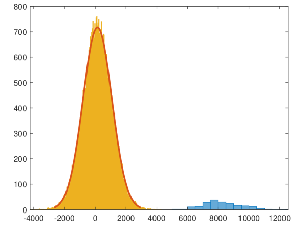
(a) Histogram of diagonal (blue) and off-diagonal (yellow with a normal fit) entries of $\widehat{X}$.

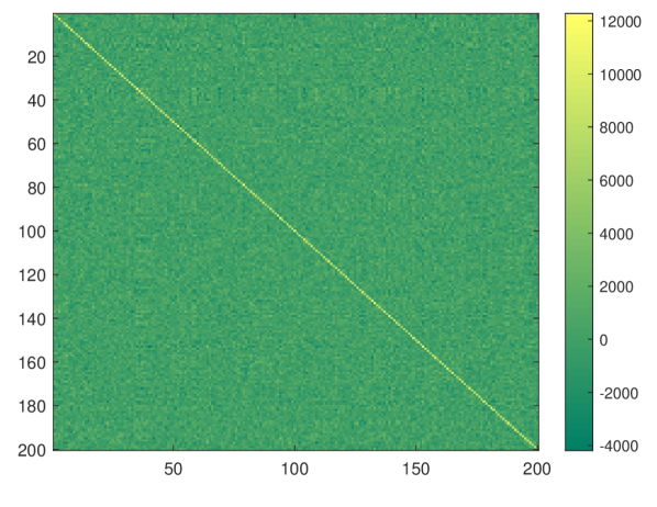
(b) Heat map of $\widehat{X}$.
 

Figure 1: Diagonal dominance of the similarity matrix $\widehat{X}$ defined by (3) or (15) for the Gaussian Wigner model $B=A+\sigma Z$ with $n=200$, $\sigma=0.05$ and $\eta=0.01$.

It is worth noting that, in contrast to the prevalent analysis of convex relaxations in statistics and machine learning (where the goal is to show that the solution to the relaxed program is close to the ground truth in a certain distance) or optimization (where the goal is to bound the gap of the objective value to the optimum), here our goal is not to show that the optimal solution per se constitutes a good estimator, but to show that it exhibits a diagonal dominance structure, which guarantees the success of the subsequent rounding procedure. For this reason, it is unclear from first principles that the guarantees obtained for one program, such as (16), automatically carry over to a tighter program, such as (14). In the companion paper [FMWX19], we analyze a tighter relaxation than (16), where the constraint is tightened to $X\mathbf{1}=\mathbf{1}$, and show that this has a similar performance guarantee; however, this requires a different analysis.

1.5 Notation

Let $[n]\triangleq\{1,\dots,n\}$. We use $C$ and $c$ to denote universal constants that may change from line to line. For two sequences $\{a_{n}\}_{n=1}^{\infty}$ and $\{b_{n}\}_{n=1}^{\infty}$ of real numbers, we write $a_{n}\lesssim b_{n}$ if there is a universal constant $C$ such that $a_{n}\leq Cb_{n}$ for all $n\geq 1$. The relation $a_{n}\gtrsim b_{n}$ is defined analogously. We write $a_{n}\asymp b_{n}$ if both the relations $a_{n}\lesssim b_{n}$ and $a_{n}\gtrsim b_{n}$ hold. Let $x\vee y=\max(x,y)$. Let $\mathsf{id}$ denote the identity permutation, i.e. $\mathsf{id}(i)=i$ for every $i$. In a Euclidean space $\mathbb{R}^{n}$ or $\mathbb{C}^{n}$, let $\mathbf{e}_{i}$ be the $i$-th standard basis vector, $\mathbf{1}=\mathbf{1}_{n}$ the all-ones vector, $\mathbf{J}=\mathbf{J}_{n}$ the $n\times n$ all-ones matrix, and $\mathbf{I}=\mathbf{I}_{n}$ the $n\times n$ identity matrix. We omit the subscripts when there is no ambiguity. Let $\|\cdot\|=\|\cdot\|_{2}$ denote the Euclidean vector norm on $\mathbb{R}^{n}$ or $\mathbb{C}^{n}$. Let $\|M\|=\max_{v\neq 0}\|Mv\|_{2}/\|v\|_{2}$ denote the Euclidean operator norm, $\|M\|_{F}=(\operatorname{Tr}M^{*}M)^{1/2}$ the Frobenius norm, and $\|M\|_{\infty}=\max_{ij}|M_{ij}|$ the elementwise $\ell_{\infty}$ norm of a matrix $M$. An eigenvector is always a unit column vector by convention. Denote by $X{\stackrel{{\scriptstyle\rm(d)}}{{=}}}Y$ if random variables $X$ and $Y$ are equal in law.

2 Main results

In this section, we formulate the models, state more precisely our main results, provide an outline of the proof, and discuss the extension to bipartite graphs.

2.1 Gaussian Wigner model

We say that $A\in\mathbb{R}^{n\times n}$ is from the Gaussian Orthogonal Ensemble, or simply $A\sim\mathsf{GOE}(n)$, if $A$ is symmetric, $\{A_{ij}:i\leq j\}$ are independent, and $A_{ij}\sim N(0,\frac{1}{n})$ for $i\neq j$ and $N(0,\frac{2}{n})$ for $i=j$. We say that the pair $A,B\in\mathbb{R}^{n\times n}$ follows the Gaussian Wigner model for graph matching if

$$B^{\pi^{*}}=A+\sigma Z,$$ (20)

where $\pi^{*}$ is an unknown permutation (ground truth), $B^{\pi^{*}}$ denotes the permuted matrix $B^{\pi^{*}}_{ij}=B_{\pi^{*}(i),\pi^{*}(j)}$, the matrices $A,Z\sim\mathsf{GOE}(n)$ are independent, and $\sigma\geq 0$ is the noise level. Our goal is to recover the latent permutation $\pi^{*}$ from $(A,B)$.

We may also consider the rescaled definition $B^{\pi^{*}}=\sqrt{1-\sigma^{2}}A+\sigma Z$, so that $A$ and $B$ have the same marginal law with correlation coefficient $1-\sigma^{2}$. Our proofs are easily adapted to this setup, and we assume (20) for simplicity and a cleaner presentation.

We now formalize the exact recovery guarantee for Algorithm 1.

Theorem 2.1.

Consider the model (20). There exist constants $c,c^{\prime}>0$ such that if

$$1/n^{0.1}\leq\eta\leq c/\log n\quad\text{ and }\quad\sigma\leq c^{\prime}\eta,$$

then with probability at least $1-n^{-4}$ for all large $n$, the matrix $\widehat{X}$ in (3) satisfies

$$\min_{i\in[n]}\widehat{X}_{i,\pi^{*}(i)}>\max_{i,j\in[n]:\,j\neq\pi^{*}(i)}\widehat{X}_{ij}$$ (21)

and hence, Algorithm 1 recovers $\widehat{\pi}=\pi^{*}$.

Choosing $\eta\asymp 1/\log n$ in Algorithm 1, we thus obtain exact recovery for $\sigma\lesssim 1/\log n$. The same exact recovery guarantee clearly also holds if rounding were performed by the simple scheme (6), instead of solving the linear assignment (5). The probability $n^{-4}$ is arbitrary and may be strengthened to $n^{-D}$ for any constant $D>0$, where $c,c^{\prime}$ above depend on $D$.

Consider next the gradient descent iterates $X^{(t)}$ defined by (17). We verify that these iterates converge to $\widehat{X}$, and that the same guarantee holds for $X^{(t)}$ for sufficiently large $t$.

Corollary 2.2.

Let $X^{(0)}=0$, define recursively $X^{(t)}$ by the gradient descent dynamics (17), and let $\widehat{X}$ be the similarity matrix (3).

1. The matrix $\widehat{X}$ is the minimizer of the unconstrained program (15), and $\alpha\widehat{X}$ is the minimizer of the constrained program (16) for some (random) scalar multiplier $\alpha>0$.

2. In terms of the spectral decompositions of $A$ and $B$ in (2), each iterate $X^{(t)}$ is given by

   $$X^{(t)}=\sum_{i,j=1}^{n}\frac{1-[1-\gamma\eta^{2}-\gamma(\lambda_{i}-\mu_{j})^{2}]^{t}}{\eta^{2}+(\lambda_{i}-\mu_{j})^{2}}u_{i}u_{i}^{\top}\mathbf{J}v_{j}v_{j}^{\top}.$$

   In particular, if the step size satisfies $\gamma<1/(\eta^{2}+(\lambda_{i}-\mu_{j})^{2})$ for all $i,j$, then $X^{(t)}\to\widehat{X}$ as $t\to\infty$.

3. In the setting of Theorem 2.1, for some constants $C,c>0$, if $\gamma<c$ and

   $$t>\frac{C\log n}{\gamma\eta^{2}},$$

   then the guarantees of Theorem 2.1 also hold with probability at least $1-n^{-4}$ with $X^{(t)}$ in place of $\widehat{X}$.

In particular, setting $\gamma$ to be a small constant and $\eta\asymp 1/\log n$, we obtain the same diagonal dominance property for $X^{(t)}$ as long as $t\gtrsim(\log n)^{3}$, and consequently either the rounding scheme (5) or (6) applied to $X^{(t)}$ recovers the true matching $\pi^{*}$.

2.2 Proof outline for Theorem 2.1

We give an outline of the proof for Theorem 2.1. By the permutation invariance property (7) of the algorithm, we may assume without loss of generality that $\pi^{*}=\mathsf{id}$, the identity permutation. Then we must show in (21) that every diagonal entry of $\widehat{X}$ is larger than every off-diagonal entry.

Denote the similarity matrix in (3) by

$$X=\widehat{X}(A,B)=\sum_{i,j=1}^{n}\frac{1}{(\lambda_{i}-\mu_{j})^{2}+\eta^{2}}u_{i}u_{i}^{\top}\mathbf{J}v_{j}v_{j}^{\top}$$ (22)

and introduce $X_{*}$ as the similarity matrix constructed in the noiseless setting with $A$ in place of $B$. That is,

$$X_{*}=\widehat{X}(A,A)=\sum_{i,j=1}^{n}\frac{1}{(\lambda_{i}-\lambda_{j})^{2}+\eta^{2}}u_{i}u_{i}^{\top}\mathbf{J}u_{j}u_{j}^{\top}.$$ (23)

We divide the proof into establishing the diagonal dominance of $X_{*}$, and then bounding the entrywise difference $X-X_{*}$.

Lemma 2.3.

For some constants $C,c>0$, if $1/n^{0.1}<\eta<c/\log n$, then with probability at least $1-5n^{-5}$ for large $n$,

$$\min_{i\in[n]}(X_{*})_{ii}>1/(3\eta^{2})$$

and

$$\max_{i,j\in[n]:i\neq j}(X_{*})_{ij}<C\left(\frac{\sqrt{\log n}}{\eta^{3/2}}+\frac{\log n}{\eta}\right).$$ (24)

Lemma 2.4.

If $\eta>1/n^{0.1}$, then for a constant $C>0$, with probability at least $1-2n^{-5}$ for large $n$,

$$\max_{i,j\in[n]}|X_{ij}-(X_{*})_{ij}|<C\sigma\left(\frac{1}{\eta^{3}}+\frac{\log n}{\eta^{2}}\left(1+\frac{\sigma}{\eta}\right)\right).$$ (25)

Proof of Theorem 2.1.

Assuming these lemmas, for some $c,c^{\prime}>0$ sufficiently small, setting $\eta<c/\log n$ and $\sigma<c^{\prime}\eta$ ensures that the right sides of both (24) and (25) are at most $1/(12\eta^{2})$. Then when $\pi^{*}=\mathsf{id}$, these lemmas combine to imply

$$\min_{i\in[n]}X_{ii}>\frac{1}{4\eta^{2}}>\frac{1}{6\eta^{2}}>\max_{i,j\in[n]:i\neq j}X_{ij}$$

with probability at least $1-n^{-4}$. On this event, by definition, both the LAP rounding procedure (5) and the simple greedy rounding (6) output $\widehat{\pi}=\mathsf{id}$. The result for general $\pi^{*}$ follows from the equivariance of the algorithm, applying this result to the inputs $A$ and $B^{\pi}$ with $\pi=(\pi^{*})^{-1}$. ∎

A large portion of the technical work will lie in establishing Lemma 2.3 for the noiseless setting. We give here a short sketch of the intuition for this lemma, ignoring momentarily any factors that are logarithmic in $n$ and are hidden by the notations $\approx$ and $\lessapprox$ below. Let us write

$$X_{*}=\sum_{i=1}^{n}\frac{1}{\eta^{2}}(u_{i}^{\top}\mathbf{J}u_{i})u_{i}u_{i}^{\top}+\sum_{i\neq j}\frac{1}{\eta^{2}+(\lambda_{i}-\lambda_{j})^{2}}(u_{i}^{\top}\mathbf{J}u_{j})u_{i}u_{j}^{\top}.$$ (26)

We explain why the first term is diagonally dominant, while the second term is a perturbation of smaller order. Central to our proof is the fact that $A\sim\mathsf{GOE}(n)$ is rotationally invariant in law, so that $U=(u_{1},\ldots,u_{n})$ is uniformly distributed on the orthogonal group and independent of $\lambda_{1},\ldots,\lambda_{n}$. The coordinates of $U$ are approximately independent with distribution $N(0,\frac{1}{n})$.

For the first term in (26), with high probability $u_{i}^{\top}\mathbf{J}u_{i}=\langle u_{i},\mathbf{1}\rangle^{2}\approx 1$ for every $i$. Then for each $k$, the $k^{\text{th}}$ diagonal entry of the first term satisfies

$$\sum_{i=1}^{n}\frac{1}{\eta^{2}}(u_{i}^{\top}\mathbf{J}u_{i})(u_{i})_{k}^{2}\approx\sum_{i=1}^{n}\frac{1}{\eta^{2}}(u_{i})_{k}^{2}\approx\frac{1}{\eta^{2}}.$$ (27)

Applying the heuristic $(u_{i})_{k}\sim N(0,\frac{1}{n})$, each $(k,\ell)^{\text{th}}$ off-diagonal entry satisfies

$$\sum_{i=1}^{n}\frac{1}{\eta^{2}}(u_{i}^{\top}\mathbf{J}u_{i})(u_{i})_{k}(u_{i})_{\ell}\lessapprox\frac{1}{\eta^{2}\sqrt{n}}.$$ (28)

For the second term in (26), each $(k,\ell)^{\text{th}}$ entry is

$$\sum_{i\neq j}\frac{1}{\eta^{2}+(\lambda_{i}-\lambda_{j})^{2}}(u_{i}^{\top}\mathbf{J}u_{j})(u_{i})_{k}(u_{j})_{\ell}=g^{\top}Qh,$$

where $Q$ is defined by $Q_{ii}=0$ and $Q_{ij}=\frac{1}{\eta^{2}+(\lambda_{i}-\lambda_{j})^{2}}(u_{i}^{\top}\mathbf{J}u_{j})$ for $i\neq j$, and the vectors $g$ and $h$ are defined by $g_{i}=(u_{i})_{k}$ and $h_{j}=(u_{j})_{\ell}$. Applying the heuristic that $g,h$ are approximately iid $N(0,\frac{1}{n}\mathbf{I})$ and approximately independent of $Q$, we have a Hanson-Wright type bound

$$g^{\top}Qh\lessapprox\frac{1}{n}\|Q\|_{F}.$$

As $n\to\infty$, the empirical spectral distribution $n^{-1}\sum_{i=1}^{n}\delta_{\lambda_{i}}$ of $A$ converges to the Wigner semicircle law with density $\rho$. Then, applying also $u_{i}^{\top}\mathbf{J}u_{j}=\langle u_{i},\mathbf{1}\rangle\langle u_{j},\mathbf{1}\rangle\lessapprox 1$, we obtain

$$\frac{1}{n^{2}}\|Q\|_{F}^{2}\lessapprox\frac{1}{n^{2}}\sum_{i\neq j}\Big{(}\frac{1}{\eta^{2}+(\lambda_{i}-\lambda_{j})^{2}}\Big{)}^{2}\approx\iint\Big{(}\frac{1}{\eta^{2}+(x-y)^{2}}\Big{)}^{2}\rho(x)\rho(y)dxdy\lessapprox\frac{1}{\eta^{3}},$$

where the last step is an elementary computation that holds for any bounded density $\rho$ with bounded support. As a result, each entry of the second term of (26) satisfies

$$\sum_{i\neq j}\frac{1}{\eta^{2}+(\lambda_{i}-\lambda_{j})^{2}}(u_{i}^{\top}\mathbf{J}u_{j})(u_{i})_{k}(u_{j})_{\ell}\lessapprox\frac{1}{\eta^{3/2}}.$$ (29)

Combining (27)–(29) shows that the noiseless solution $X_{*}$ in (26) is indeed diagonally dominant, with diagonals approximately $\eta^{-2}$ and off-diagonals at most of the order $\eta^{-3/2}$, omitting logarithmic factors. We carry out this proof more rigorously in Section 3.1 to establish Lemma 2.3.

2.3 Gaussian bipartite model

Consider the following asymmetric variant of this problem: Let $F,G\in\mathbb{R}^{n\times m}$ be adjacency matrices of two weighted bipartite graphs on $n$ left vertices and $m$ right vertices, where $m\geq n$ is assumed without loss of generality. Suppose, for latent permutations $\pi_{1}^{*}$ on $[n]$ and $\pi_{2}^{*}$ on $[m]$, that $\{(F_{ij},G_{\pi_{1}^{*}(i),\pi_{2}^{*}(j)}):1\leq i\leq n,1\leq j\leq m\}$ are i.i.d. pairs of correlated random variables. We wish to recover $(\pi_{1}^{*},\pi_{2}^{*})$ from $F$ and $G$.

We propose to apply Algorithm 1 on the left singular values and singular vectors of $F$ and $G$ to first recover the (smaller) row permutation $\pi_{1}^{*}$, and then solve a second LAP to recover the (bigger) column permutation $\pi_{2}^{*}$. This is summarized as follows:

Algorithm 2 Bi-GRAMPA (Bipartite GRAph Matching by Pairwise eigen-Alignments)

1:  Input: $F,G\in{\mathbb{R}}^{n\times m}$, a tuning parameter $\eta>0$.

2:  Output: Row permutation $\widehat{\pi}_{1}\in\mathcal{S}_{n}$ and column permutation $\widehat{\pi}_{2}\in\mathcal{S}_{m}$.

3:  Construct the similarity matrix $\widehat{X}$ as in (3), where now $\lambda_{1}\geq\ldots\geq\lambda_{n}$ and $\mu_{1}\geq\ldots\geq\mu_{n}$ are the singular values of $F$ and $G$, and $u_{i}$ and $v_{j}$ are the corresponding left singular vectors.

4:  Let $\widehat{\pi}_{1}$ be the estimate in (5), and denote by $G^{\widehat{\pi}_{1},\mathsf{id}}\in\mathbb{R}^{n\times m}$ the matrix $G^{\widehat{\pi}_{1},\mathsf{id}}_{ij}=G_{\widehat{\pi}_{1}(i),j}$.

5:  Find $\widehat{\pi}_{2}$ by solving the linear assignment problem

$$\widehat{\pi}_{2}=\operatorname*{argmax}_{\pi\in\mathcal{S}_{m}}\sum_{j=1}^{m}(F^{\top}G^{\widehat{\pi}_{1},\mathsf{id}})_{j,\pi(j)}.$$ (30)

We also establish an exact recovery guarantee for this method in a Gaussian setting: We say that the pair $F,G\in\mathbb{R}^{n\times m}$ follows the Gaussian bipartite model for graph matching if

$$G^{\pi_{1}^{*},\pi_{2}^{*}}=F+\sigma W,$$ (31)

where $G^{\pi_{1}^{*},\pi_{2}^{*}}$ denotes the permuted matrix $G^{\pi_{1}^{*},\pi_{2}^{*}}_{ij}=G_{\pi_{1}^{*}(i),\pi_{2}^{*}(j)}$, the matrices $F$ and $W$ are independent with i.i.d. $N(0,\frac{1}{m})$ entries, and $\sigma\geq 0$ is the noise level. We assume the asymptotic regime

$$m=m(n)\quad\text{ and }\quad n/m\to\kappa\in(0,1]\quad\text{ as }\quad n\to\infty.$$ (32)

Theorem 2.5.

Consider the model (31), where $n/m\to\kappa\in(0,1]$. There exist $\kappa$-dependent constants $c,c^{\prime}>0$ such that if

$$1/n^{0.1}\leq\eta\leq c/\log n\quad\text{ and }\quad\sigma\log(1/\sigma)\leq c^{\prime}\eta/\log n,$$

then with probability at least $1-n^{-4}$ for all large $n$, Algorithm 2 recovers $(\widehat{\pi}_{1},\widehat{\pi}_{2})=(\pi_{1}^{*},\pi_{2}^{*})$.

Setting $\eta\asymp 1/\log n$, we obtain exact recovery under the condition $\sigma\lesssim(\log n)^{-2}(\log\log n)^{-1}$.

The proof is an extension of that of Theorem 2.1: Note that the first step of Algorithm 2 is equivalent to applying Algorithm 1 on the symmetric polar parts $A=\sqrt{FF^{\top}}$ and $B=\sqrt{GG^{\top}}$, where $\sqrt{\cdot}$ denotes the symmetric matrix square root. In the Gaussian setting, $A$ is still rotationally invariant, and Lemma 2.3 will extend directly to $X_{*}$ constructed from this $A$. We will show a simpler and slightly weaker version of Lemma 2.4 to establish exact recovery of the left permutation $\pi_{1}^{*}$, under the stronger requirement for $\sigma$ above. We will then analyze separately the linear assignment for recovering $\pi_{2}^{*}$. Details of the argument are provided in Section 3.3.

We conclude this section by discussing the assumption (32). The condition $n\to\infty$ is information-theoretically necessary to recover the right permutation $\pi_{2}^{*}$, unless $\sigma$ is as small as $1/\mathrm{poly}(n)$. This can be seen by considering the oracle setting when $\pi_{1}^{*}$ is given, in which case the necessary and sufficient condition for the maximal likelihood (linear assignment) to succeed is given by $n\log\left(1+\frac{1}{\sigma^{2}}\right)-4\log m\to\infty$ [DCK19]. The condition of finite aspect ratio $n=\Theta(m)$ is assumed for the analysis of the Bi-GRAMPA algorithm; otherwise, if $n=o(m)$, then the empirical distribution of singular values of $F$ converges to a point mass at $1$, and it is unclear whether the spectral similarity matrix in (22) or (23) continues to be diagonally dominant. We note that such a condition is not information-theoretically necessary. In fact, as long as $n$ and $m$ are polynomially related, running the degree profile matching algorithm [DMWX18, Section 2] on the row-wise and column-wise empirical distributions succeeds for $\sigma=O(\frac{1}{\log n})$.

3 Proofs

We prove our main results in this section. Section 3.1 proves Lemma 2.3, which shows the diagonal dominance of $X_{*}$ in the noiseless setting of $A=B$. Section 3.2 proves Lemma 2.4, which bounds the difference $X-X_{*}$. Together with the argument in Section 2.2, these yield Theorem 2.1 on the exact recovery in the Gaussian Wigner model.

Section 3.3 extends this analysis to establish Theorem 2.5 for the bipartite model. Finally, Section 3.4 (which may be read independently) proves Corollary 2.2 relating $\widehat{X}$ to the gradient descent dynamics (17) and the optimization problems (15) and (16).

3.1 Analysis in the noiseless setting

We first prove Lemma 2.3, showing diagonal dominance in the noiseless setting. Throughout, we write the spectral decomposition

$$A=U\Lambda U^{\top}\quad\text{ where }\quad U=[u_{1}\cdots u_{n}]\text{ and }\Lambda=\mathsf{diag}(\lambda_{1},\dots,\lambda_{n}).$$ (33)

3.1.1 Properties of $A$ and rotation by $U$

In the proof, we will in fact only use the properties of the matrix $A\sim\mathsf{GOE}(n)$ recorded in the following proposition. The same proof will then apply to the bipartite case wherein the suitably defined $A$ satisfies the same properties.

Proposition 3.1.

Suppose $A\sim\mathsf{GOE}(n)$. Then for constants $C,c>0$,

1. $U$ is a uniform random orthogonal matrix independent of $\Lambda$.

2. The empirical spectral distribution $\rho_{n}=\frac{1}{n}\sum_{i=1}^{n}\delta_{\lambda_{i}}$ of $A$ converges to a limiting law $\rho$, which has a density function bounded by $C$ and support contained in $[-C,C]$. Moreover, for all large $n$,

   $$\mathbb{P}\Big{\{}\sup_{x}|F_{n}(x)-F(x)|>Cn^{-1}(\log n)^{5}\Big{\}}<n^{-c\log\log n},$$

   where $F_{n}$ and $F$ are the cumulative distribution functions of $\rho_{n}$ and $\rho$ respectively.

3. For all large $n$, $\mathbb{P}\big{\{}\|A\|>C\}<e^{-cn}$.

Proof.

Parts (a) and (c) are well-known, see for example [AGZ10, Corollary 2.5.4 and Lemma 2.6.7]. For (b), $\rho$ is the Wigner semicircle law on $[-2,2]$, and the rate of convergence follows from [GT13, Theorem 1.1]. ∎

Recall the definition

$$X_{*}=\sum_{i,j=1}^{n}\frac{1}{\eta^{2}+(\lambda_{i}-\lambda_{j})^{2}}u_{i}u_{i}^{\top}\mathbf{J}u_{j}u_{j}^{\top}.$$

Our goal is to exhibit the diagonal dominance of this matrix. Without loss of generality, we analyze $(X_{*})_{11}=\mathbf{e}_{1}^{\top}X_{*}\mathbf{e}_{1}$ and $(X_{*})_{12}=\mathbf{e}_{1}^{\top}X_{*}\mathbf{e}_{2}$.

Applying Proposition 3.1 (a) above, let us rotate by $U$ to write the quantities of interest in a more convenient form. Namely, we set

$$\varphi=U^{\top}\mathbf{e}_{1},\quad\psi=U^{\top}\mathbf{e}_{2},\quad\text{and}\quad\xi=U^{\top}\mathbf{1}.$$ (34)

These vectors satisfy

$$\|\varphi\|_{2}=\|\psi\|_{2}=1,\quad\|\xi\|_{2}=\sqrt{n},\quad\langle\varphi,\xi\rangle=1,\quad\langle\psi,\xi\rangle=1,\quad\text{and}\quad\langle\varphi,\psi\rangle=0,$$ (35)

and are otherwise “uniformly random”. By this, we mean that $(\varphi,\psi,\xi)$ is equal in law to $(O\varphi,O\psi,O\xi)$ for any orthogonal matrix $O\in\mathbb{R}^{n\times n}$, which follows from Proposition 3.1(a).

Define a symmetric matrix $L\in\mathbb{R}^{n\times n}$ by

$$L_{ij}=\frac{1}{\eta^{2}+(\lambda_{i}-\lambda_{j})^{2}},$$ (36)

and define $\widetilde{L}\in\mathbb{R}^{n\times n}$ such that $\widetilde{L}_{ii}=0$ and $\widetilde{L}_{ij}=L_{ij}$ for $i\neq j$. Then

$$(X_{*})_{12}=\sum_{i,j=1}^{n}L_{ij}\varphi_{i}\psi_{j}\xi_{i}\xi_{j},$$ (37)

and

$$(X_{*})_{11}=\frac{1}{\eta^{2}}\sum_{i=1}^{n}\varphi_{i}^{2}\xi_{i}^{2}+\sum_{i,j=1}^{n}\widetilde{L}_{ij}\varphi_{i}\varphi_{j}\xi_{i}\xi_{j}.$$ (38)

Importantly, by Proposition 3.1(a), the triple $(\varphi,\psi,\xi)$ is independent of $L$ and $\widetilde{L}$. We will establish the following technical lemmas.

Lemma 3.2.

With probability at least $1-3n^{-7}$ for large $n$,

$$\sum_{i=1}^{n}\varphi_{i}^{2}\xi_{i}^{2}>\frac{1}{2}.$$

Lemma 3.3.

For some constants $C,c>0$, if $1/n^{0.1}<\eta<c$, then with probability at least $1-2n^{-7}$ for large $n$,

$$\Big{|}\sum_{i,j=1}^{n}L_{ij}\varphi_{i}\psi_{j}\xi_{i}\xi_{j}\Big{|}\lor\Big{|}\sum_{i,j=1}^{n}\widetilde{L}_{ij}\varphi_{i}\varphi_{j}\xi_{i}\xi_{j}\Big{|}<C\left(\frac{\sqrt{\log n}}{\eta^{3/2}}+\frac{\log n}{\eta}\right).$$ (39)

Lemma 2.3 follows immediately from these results. Indeed, for $\eta<c/\log n$ and sufficiently small $c>0$, these results and the forms (37–38) combine to yield $(X_{*})_{11}>1/(3\eta^{2})$ and $(X_{*})_{12}<C(\sqrt{\log n}/\eta^{3/2}+(\log n)/\eta)$ with probability at least $1-5n^{-7}$. By symmetry, the same result holds for all $(X_{*})_{ii}$ and $(X_{*})_{ij}$, and Lemma 2.3 follows from taking a union bound over $i$ and $j$.

It remains to show Lemmas 3.2 and 3.3. The general strategy is to approximate the law of $(\varphi,\psi,\xi)$ by suitably defined Gaussian random vectors, and then to apply Gaussian tail bounds and concentration inequalities which are collected in Appendix A. As an intermediate step, we will show the following estimates for the matrix $L$, using the convergence of the empirical spectral distribution in Proposition 3.1(b).

Lemma 3.4.

For constants $C,c>0$, with probability at least $1-n^{-10}$ for large $n$,

$$\min_{i,j\in[n]}L_{ij}\geq c,\quad\max_{i,j\in[n]}L_{ij}\leq\frac{1}{\eta^{2}},\quad\frac{1}{n}\|L\|_{F}\leq\frac{C}{\eta^{3/2}},$$

$$\frac{1}{n}\max_{i\in[n]}\sum_{j=1}^{n}L_{ij}^{2}\leq\frac{C}{\eta^{3}}\quad\text{ and }\quad\frac{1}{n}\max_{i\in[n]}\sum_{j=1}^{n}L_{ij}\leq\frac{C}{\eta}.$$

3.1.2 Proof of Lemma 3.2

Let $z$ be a standard Gaussian vector in $\mathbb{R}^{n}$ independent of $\varphi$. First, we note that marginally $\varphi$ is equal to $z/\|z\|_{2}$ in law. By standard bounds on $\max_{j}|z_{j}|$ and $\|z\|_{2}$ (see Lemmas A.1 and A.3), we have that with probability at least $1-2n^{-7}$,

$$\max_{i\in[n]}\big{|}\varphi_{i}\big{|}\leq 5\left(\frac{\log n}{n}\right)^{1/2}.$$ (40)

Next, the random vectors $\varphi$ and $\xi$ satisfy that $\|\varphi\|_{2}=1$, $\|\xi\|_{2}=\sqrt{n}$ and $\langle\varphi,\xi\rangle=1$, and are otherwise uniformly random. Hence if we let $z$ be a standard Gaussian vector in $\mathbb{R}^{n}$ and define

$$\widetilde{\xi}\triangleq\sqrt{n-1}\,\frac{z-(\varphi^{\top}z)\varphi}{\big{\|}z-(\varphi^{\top}z)\varphi\big{\|}_{2}}+\varphi,$$

then $(\varphi,\xi){\stackrel{{\scriptstyle\rm(d)}}{{=}}}(\varphi,\widetilde{\xi})$. Note that we can write $\widetilde{\xi}=\alpha z+\beta\varphi$, where $\alpha$ and $\beta=1-\alpha(\varphi^{\top}z)$ are random variables satisfying $0.9\leq\alpha\leq 1.1$ and $|\beta|\leq 4\sqrt{\log n}$ with probability at least $1-4n^{-8}$ by concentration of $\|z\|_{2}$ and $\varphi^{\top}z$ (Lemmas A.1 and A.3). Therefore, we obtain

$$\sum_{i=1}^{n}\varphi_{i}^{2}\widetilde{\xi}_{i}^{2}=\sum_{i=1}^{n}\varphi_{i}^{2}\left(\alpha^{2}z_{i}^{2}+\beta^{2}\varphi_{i}^{2}+2\alpha\beta z_{i}\varphi_{i}\right)\geq 0.8\sum_{i=1}^{n}\varphi_{i}^{2}z_{i}^{2}-9\sqrt{\log n}\left|\sum_{i=1}^{n}\varphi_{i}^{3}z_{i}\right|.$$ (41)

For the first term of (41), applying Lemma A.3 and then (40) yields

$$\sum_{i=1}^{n}\varphi_{i}^{2}z_{i}^{2}\geq 1-22(\log n)\left(\sum_{i=1}^{n}\varphi_{i}^{4}\right)^{1/2}\geq 1-22(\log n)\left(\sum_{i=1}^{n}5^{4}\left(\frac{\log n}{n}\right)^{2}\right)^{1/2}\geq 0.9$$

with probability at least $1-3n^{-7}$. For the second term of (41), we once again apply Lemma A.1 and then (40) to obtain

$$9\sqrt{\log n}\Big{|}\sum_{i=1}^{n}\varphi_{i}^{3}z_{i}\Big{|}\leq 20\log n\left(\sum_{i=1}^{n}\varphi_{i}^{6}\right)^{\frac{1}{2}}\leq 0.1$$

with probability at least $1-3n^{-7}$. Combining the three terms finishes the proof.

3.1.3 Proof of Lemma 3.4

Let $\rho_{n}$ be the empirical spectral distribution of $A$. For a large enough constant $C_{1}>0$ where $[-C_{1},C_{1}]$ contains the support of $\rho$, let $\mathcal{E}$ be the event where it also contains the support of $\rho_{n}$, and

$$\sup_{x}|F_{n}(x)-F(x)|<n^{-0.5}.$$ (42)

By Proposition 3.1, $\mathcal{E}$ holds with probability at least $1-n^{-10}$.

The bound $L_{ij}\leq 1/\eta^{2}$ holds by the definition (36). The bound $n^{-1}\|L\|_{F}\leq C\eta^{-3/2}$ follows from summing $n^{-1}\sum_{j}L_{ij}^{2}\leq C\eta^{-3}$ also over $i$ and taking a square root. The bound $c\leq L_{ij}$ also holds on $\mathcal{E}$ by the definition of $L$. It remains to prove the last two bounds on the rows of $L$.

For this, fix $a=1$ or $a=2$. For each $\lambda\in[-C_{1},C_{1}]$, define a function

$$g_{\lambda}(r)\triangleq\left(\frac{1}{\eta^{2}+(r-\lambda)^{2}}\right)^{a}.$$

Then for each $i$,

$$\frac{1}{n}\sum_{j=1}^{n}L_{ij}^{a}=\frac{1}{n}\sum_{j=1}^{n}g_{\lambda_{i}}(\lambda_{j})=\int_{-C_{1}}^{C_{1}}g_{\lambda_{i}}(r)d\rho_{n}(r).$$ (43)

For some constants $C,C^{\prime}>0$ and every $\lambda\in[-C_{1},C_{1}]$, replacing $\rho_{n}$ by the limiting density $\rho$, we have

$$\int_{-C_{1}}^{C_{1}}g_{\lambda}(r)d\rho(r) \leq C\int_{-C_{1}}^{C_{1}}\left(\frac{1}{\eta^{2}+(r-\lambda)^{2}}\right)^{a}dr$$

$$\leq C\left(\int_{|r-\lambda|\leq\eta}\frac{1}{\eta^{2a}}dr+\int_{\eta\leq|r-\lambda|\leq 2C_{1}}\frac{1}{(r-\lambda)^{2a}}dr\right)\leq C^{\prime}\eta^{1-2a}.$$ (44)

To bound the difference between $\rho_{n}$ and $\rho$, note that $g_{\lambda}(r)\geq y$ for $y\geq 0$ if and only if $|r-\lambda|\leq b$ for some $b=b(y)\geq 0$. Consider random variables $R_{n}\sim\rho_{n}$ and $R\sim\rho$. Since $g_{\lambda}\leq\eta^{-2a}$, we have

$$\Big{|}\int_{-C_{1}}^{C_{1}}g_{\lambda}(r)d\rho_{n}(r)-\int_{-C_{1}}^{C_{1}}g_{\lambda}(r)d\rho(r)\Big{|}$$

$$=\Big{|}\int_{0}^{\eta^{-2a}}\left(\mathbb{P}\big{\{}g_{\lambda}(R_{n})\geq y\big{\}}-\mathbb{P}\big{\{}g_{\lambda}(R)\geq y\big{\}}\right)dy\Big{|}$$

$$\leq\int_{0}^{\eta^{-2a}}\Big{|}\mathbb{P}\big{\{}|R_{n}-\lambda|\leq b(y)\big{\}}-\mathbb{P}\big{\{}|R-\lambda|\leq b(y)\big{\}}\Big{|}dy$$

$$\leq\int_{0}^{\eta^{-2a}}2n^{-0.5}dy=2\eta^{-2a}n^{-0.5},$$

where the last inequality holds on the event $\mathcal{E}$ by (42). Combining the last display with (44), we get that (43) is at most $C\eta^{1-2a}$ for $\eta>n^{-0.1}$. This gives the desired bounds for $a=1$ and $a=2$.

3.1.4 Proof of Lemma 3.3

We now use Lemma 3.4 to prove Lemma 3.3. Recall $L$ defined in (36), and $\widetilde{L}$ which sets its diagonal to 0. We need to bound the quantities

$$\text{(I)}:\sum_{i,j=1}^{n}L_{ij}\varphi_{i}\psi_{j}\xi_{i}\xi_{j}\quad\text{ and }\quad\text{(II)}:\sum_{i,j=1}^{n}\widetilde{L}_{ij}\varphi_{i}\varphi_{j}\xi_{i}\xi_{j}.$$ (45)

The proof for (II) is almost the same as that for (I), so we focus on (I) and briefly discuss the differences for (II). Let us define a matrix $K\in\mathbb{R}^{n\times n}$ by setting

$$K_{ij}=L_{ij}\varphi_{i}\psi_{j}.$$ (46)

Estimates for $K$.

We translate the estimates for $L$ in Lemma 3.4 to ones for $K$. Note that since $\varphi$ and $\psi$ are independent of $L$ and uniform over the sphere with entries on the order of $\frac{1}{\sqrt{n}}$, it is reasonable to expect that $\|K\|_{F}\lesssim\frac{1}{n}\|L\|_{F}$ and $\|K\|\lesssim\frac{1}{n}\|L\|$ with high probability; however, neither statement is true in general, as shown by the counterexamples $L=\mathbf{e}_{1}\mathbf{e}_{1}^{\top}$ and $L=\mathbf{I}$. Fortunately, both statements hold for $L$ defined by (36) thanks to the structural properties established in Lemma 3.4.

Lemma 3.5.

In the setting of Lemma 3.3, for the matrix $K\in\mathbb{R}^{n\times n}$ defined by (46), we have $\|K\|_{F}\lesssim\frac{1}{\eta^{3/2}}$ with probability at least $1-2n^{-8}$.

Proof.

It suffices to prove that conditional on $L$, with probability at least $1-n^{-8}$, we have

$$\|K\|_{F}\lesssim\frac{1}{n}\|L\|_{F}+\frac{\log n}{n^{1/4}}\|L\|_{\infty}.$$

This together with Lemma 3.4 yields that

$$\|K\|_{F}\lesssim\frac{1}{\eta^{3/2}}+\frac{\log n}{n^{1/4}\eta^{2}}\lesssim\frac{1}{\eta^{3/2}},$$

where the last inequality holds since we choose $\eta\gtrsim n^{-0.1}$.

Note that we have

$$\|K\|_{F}^{2}=\sum_{i,j=1}^{n}\varphi_{i}^{2}\psi_{j}^{2}L_{ij}^{2}\leq\frac{1}{2}\sum_{i,j=1}^{n}\varphi_{i}^{4}L_{ij}^{2}+\frac{1}{2}\sum_{i,j=1}^{n}\psi_{j}^{4}L_{ij}^{2}.$$

It suffices to bound the first term, as the second term has the same distribution. Let $z$ be a standard Gaussian vector in $\mathbb{R}^{n}$. Then $z/\|z\|_{2}{\stackrel{{\scriptstyle\rm(d)}}{{=}}}\varphi$. By the concentration of $\|z\|_{2}$ around $\sqrt{n}$ (Lemma A.3), it remains to prove that with probability at least $1-n^{-10}$,

$$\sum_{i,j=1}^{n}z_{i}^{4}L_{ij}^{2}=\sum_{i=1}^{n}z_{i}^{4}\alpha_{i}\lesssim\|L\|_{F}^{2}+\|L\|_{\infty}^{2}n^{3/2}(\log n)^{2}$$

where $\alpha_{i}\triangleq\sum_{j=1}^{n}L_{ij}^{2}$.

To this end, we compute

$$\mathbb{E}\left[\sum_{i=1}^{n}z_{i}^{4}\alpha_{i}\right]=3\|L\|_{F}^{2}$$

and moreover

$$\mathsf{Var}\left(\sum_{i=1}^{n}z_{i}^{4}\alpha_{i}\right) =\sum_{i=1}^{n}\mathsf{Var}(z_{i}^{4})\alpha_{i}^{2}=105\sum_{i=1}^{n}\alpha_{i}^{2}\lesssim n^{3}\|L\|_{\infty}^{4}.$$

Therefore, applying Theorem A.4 with $d=4$ we obtain

$$\left|\sum_{i=1}^{n}z_{i}^{4}\alpha_{i}^{2}-3\|L\|_{F}^{2}\right|\lesssim\|L\|_{\infty}^{2}n^{3/2}(\log n)^{2}$$

with probability at least $1-n^{-10}$, which completes the proof. ∎

Lemma 3.6.

It holds with probability at least $1-n^{-8}$ that for all $j,k\in[n]$,

$$\sum_{i=1}^{n}\varphi_{i}^{2}L_{ij}L_{ik}\lesssim\frac{1}{n}\sum_{i=1}^{n}L_{ij}L_{ik}\quad\text{ and }\quad\sum_{i=1}^{n}\psi_{i}^{2}L_{ij}\lesssim\frac{1}{\eta}.$$

Proof.

Since $z/\|z\|_{2}$ has the same distribution as $\varphi$ or $\psi$. By the concentration of $\|z\|_{2}$ around $\sqrt{n}$ (Lemma A.3) and a union bound, it remains to prove that with probability at least $1-n^{-10}$,

$$\sum_{i=1}^{n}z_{i}^{2}L_{ij}L_{ik}\lesssim\sum_{i=1}^{n}L_{ij}L_{ik}\quad\text{ and }\quad\sum_{i=1}^{n}z_{i}^{2}L_{ij}\lesssim\frac{n}{\eta}.$$ (47)

For the first inequality, Lemma A.3 gives that with probability at least $1-n^{-11}$,

$$\sum_{i=1}^{n}z_{i}^{2}L_{ij}L_{ik}\lesssim\sum_{i=1}^{n}L_{ij}L_{ik}+\left(\sum_{i=1}^{n}L_{ij}^{2}L_{ik}^{2}\log n\right)^{1/2}+\left(\max_{i\in[n]}L_{ij}L_{ik}\right)\log n.$$

Note that $1\lesssim L_{ij}\leq 1/\eta^{2}$ by Lemma 3.4, so

$$\sum_{i=1}^{n}L_{ij}L_{ik}\gtrsim n\quad\text{ and }\quad\left(\sum_{i=1}^{n}L_{ij}^{2}L_{ik}^{2}\log n\right)^{1/2}+\left(\max_{i\in[n]}L_{ij}L_{ik}\right)\log n\lesssim\frac{\sqrt{n\log n}}{\eta^{4}}+\frac{\log n}{\eta^{4}}.$$

Therefore, if $\eta\gtrsim n^{-0.1}$, then $\sum_{i=1}^{n}L_{ij}L_{ik}$ is the dominating term. Hence the first bound in (47) is established.

The same argument also works to yield

$$\sum_{i=1}^{n}z_{i}^{2}L_{ij}\lesssim\sum_{i=1}^{n}L_{ij}.$$

Combining this with Lemma 3.4, we obtain the second bound in (47). ∎

Lemma 3.7.

For the matrix $K\in\mathbb{R}^{n\times n}$ defined by (46), we have $\|K\|\lesssim 1/\eta$ with probability at least $1-2n^{-8}$.

Proof.

Consider the event where the estimates of Lemmas 3.4 and 3.6 hold. Fix a unit vector $x\in\mathbb{R}^{n}$. We have

$$\|Kx\|_{2}^{2}=\sum_{i=1}^{n}\left(\sum_{j=1}^{n}\varphi_{i}\psi_{j}L_{ij}x_{j}\right)^{2}=\sum_{j,k=1}^{n}\left(\sum_{i=1}^{n}\varphi_{i}^{2}L_{ij}L_{ik}\right)\psi_{j}\psi_{k}x_{j}x_{k}.$$

The first bound in Lemma 3.6 then yields that

$$\|Kx\|_{2}^{2} \lesssim\frac{1}{n}\sum_{j,k=1}^{n}\left(\sum_{i=1}^{n}L_{ij}L_{ik}\right)|\psi_{j}\psi_{k}x_{j}x_{k}|$$

$$=\frac{1}{n}\sum_{i=1}^{n}\left(\sum_{j=1}^{n}|\psi_{j}|L_{ij}|x_{j}|\right)^{2}=\frac{1}{n}\big{\|}M|x|\big{\|}_{2}^{2}\leq\frac{1}{n}\|M\|^{2},$$ (48)

where $|x|$ denotes the vector whose $i$-th entry is $|x_{i}|$, and the matrix $M$ is defined by

$$M_{ij}=|\psi_{j}|L_{ij}.$$

Moreover, we have that

$$\|M^{\top}x\|_{2}^{2}=\sum_{i=1}^{n}\psi_{i}^{2}\left(\sum_{j=1}^{n}L_{ij}x_{j}\right)^{2}\leq\sum_{i=1}^{n}\psi_{i}^{2}\left(\sum_{j=1}^{n}L_{ij}\right)\left(\sum_{j=1}^{n}L_{ij}x_{j}^{2}\right)\lesssim\frac{n}{\eta}\sum_{j=1}^{n}\left(\sum_{i=1}^{n}\psi_{i}^{2}L_{ij}\right)x_{j}^{2},$$

where the first inequality follows from the Cauchy-Schwarz inequality, and the second inequality follows from the row sum bound in Lemma 3.4. In addition, by the second inequality in Lemma 3.6,

$$\|M^{\top}x\|_{2}^{2}\lesssim\frac{n}{\eta^{2}}\sum_{j=1}^{n}x_{j}^{2}=\frac{n}{\eta^{2}}.$$

It follows that $\|M\|^{2}=\|M^{\top}\|^{2}\lesssim n/\eta^{2}$ which, combined with (48), yields $\|Kx\|_{2}^{2}\lesssim 1/\eta^{2}$. Therefore, we conclude that $\|K\|\lesssim 1/\eta.$ ∎

Bounding (I).

We now bound $\sum_{i,j=1}^{n}L_{ij}\varphi_{i}\psi_{j}\xi_{i}\xi_{j}$. Recall that the vectors $\varphi,\psi$ and $\xi$ satisfy the relations (35) and are otherwise uniform random. Let $z$ be a standard Gaussian vector in $\mathbb{R}^{n}$ independent of $(\varphi,\psi)$ and define

$$\widetilde{\xi}\triangleq\sqrt{n-2}\,\frac{z-(\varphi^{\top}z)\varphi-(\psi^{\top}z)\psi}{\big{\|}z-(\varphi^{\top}z)\varphi-(\psi^{\top}z)\psi\big{\|}_{2}}+\varphi+\psi.$$ (49)

Then the tuple $(\varphi,\psi,\widetilde{\xi})$ is equal to $(\varphi,\psi,\xi)$ in law. Thus it suffices to study

$$\sum_{i,j=1}^{n}L_{ij}\varphi_{i}\psi_{j}\widetilde{\xi}_{i}\widetilde{\xi}_{j}.$$

Note that we can write $\widetilde{\xi}=\alpha z+\beta_{1}\varphi+\beta_{2}\psi$ for random variables $\alpha,\beta_{1},\beta_{2}\in\mathbb{R}$, where $\beta_{1}=1-\alpha(\varphi^{\top}z)$ and $\beta_{2}=1-\alpha(\psi^{\top}z)$. By concentration inequalities for $\|z\|_{2}$ and $\varphi^{\top}z$ (Lemmas A.1 and A.3), we have $0.9\leq\alpha\leq 1.1$ and $|\beta_{1}|\lor|\beta_{2}|\leq 5\sqrt{\log n}$ with probability at least $1-4n^{-8}$. Therefore, we obtain

$$\left|\sum_{i,j=1}^{n}L_{ij}\varphi_{i}\psi_{j}\widetilde{\xi}_{i}\widetilde{\xi}_{j}\right|\lesssim\left|\sum_{i,j=1}^{n}L_{ij}\varphi_{i}\psi_{j}z_{i}z_{j}\right|+\sqrt{\log n}\left|\sum_{i,j=1}^{n}L_{ij}\varphi_{i}\varphi_{j}\psi_{j}z_{i}\right|+\sqrt{\log n}\left|\sum_{i,j=1}^{n}L_{ij}\varphi_{i}\psi_{j}^{2}z_{i}\right|$$

$$\qquad\qquad+\sqrt{\log n}\left|\sum_{i,j=1}^{n}L_{ij}\varphi_{i}^{2}\psi_{j}z_{j}\right|+\sqrt{\log n}\left|\sum_{i,j=1}^{n}L_{ij}\varphi_{i}\psi_{i}\psi_{j}z_{j}\right|+(\log n)\left|\sum_{i,j=1}^{n}L_{ij}\varphi_{i}^{2}\varphi_{j}\psi_{j}\right|$$

$$\qquad\qquad+(\log n)\left|\sum_{i,j=1}^{n}L_{ij}\varphi_{i}^{2}\psi_{j}^{2}\right|+(\log n)\left|\sum_{i,j=1}^{n}L_{ij}\varphi_{i}\varphi_{j}\psi_{i}\psi_{j}\right|+(\log n)\left|\sum_{i,j=1}^{n}L_{ij}\varphi_{i}\psi_{i}\psi_{j}^{2}\right|.$$ (50)

By the symmetry of $\varphi$ and $\psi$, it suffices to study the following quantities

$$(\text{i}):\sum_{i,j=1}^{n}L_{ij}\varphi_{i}\psi_{j}z_{i}z_{j},\quad(\text{ii}):\sum_{i,j=1}^{n}L_{ij}\varphi_{i}\varphi_{j}\psi_{j}z_{i},\quad(\text{iii}):\sum_{i,j=1}^{n}L_{ij}\varphi_{i}\psi_{j}^{2}z_{i},$$

$$(\text{iv}):\sum_{i,j=1}^{n}L_{ij}\varphi_{i}^{2}\varphi_{j}\psi_{j},\quad(\text{v}):\sum_{i,j=1}^{n}L_{ij}\varphi_{i}^{2}\psi_{j}^{2},\qquad(\text{vi}):\sum_{i,j=1}^{n}L_{ij}\varphi_{i}\varphi_{j}\psi_{i}\psi_{j}.$$ (51)

We now bound each of these sums.

Bounding (i). For the matrix $K$ defined by (46), Lemma A.2 yields that

$$\left|\sum_{i,j=1}^{n}L_{ij}\varphi_{i}\psi_{j}z_{i}z_{j}\right|=|z^{\top}Kz|\lesssim|\operatorname{Tr}(K)|+\|K\|_{F}\sqrt{\log n}+\|K\|\log n,$$

with probability at least $1-n^{-10}$. The trace vanishes because

$$\operatorname{Tr}(K)=\sum_{i=1}^{n}L_{ii}\varphi_{i}\psi_{i}=\frac{1}{\eta^{2}}\langle\varphi,\psi\rangle=\frac{1}{\eta^{2}}\langle U^{\top}\mathbf{e}_{1},U^{\top}\mathbf{e}_{2}\rangle=0.$$

Moreover, Lemmas 3.5 and 3.7 imply that with probability at least $1-4n^{-8}$, we have $\|K\|_{F}\lesssim 1/\eta^{3/2}$ and $\|K\|\lesssim 1/\eta$. Therefore, we conclude that

$$\left|\sum_{i,j=1}^{n}L_{ij}\varphi_{i}\psi_{j}z_{i}z_{j}\right|\lesssim\frac{\sqrt{\log n}}{\eta^{3/2}}+\frac{\log n}{\eta}.$$

Bounding (ii) and (iii). For (ii) in (51), Lemma A.1 gives that with probability at least $1-n^{-10}$,

$$\left|\sum_{i,j=1}^{n}L_{ij}\varphi_{i}\varphi_{j}\psi_{j}z_{i}\right|\lesssim\left[\sum_{i=1}^{n}\varphi_{i}^{2}\left(\sum_{j=1}^{n}L_{ij}\varphi_{j}\psi_{j}\right)^{2}\right]^{1/2}\sqrt{\log n}.$$

Applying Lemmas 3.6 and 3.4, we obtain that with probability at least $1-3n^{-8}$,

$$\left|\sum_{j=1}^{n}L_{ij}\varphi_{j}\psi_{j}\right|\leq\frac{1}{2}\sum_{j=1}^{n}L_{ij}\varphi_{j}^{2}+\frac{1}{2}\sum_{j=1}^{n}L_{ij}\psi_{j}^{2}\lesssim\frac{1}{n}\sum_{j=1}^{n}L_{ij}\lesssim\frac{1}{\eta}.$$

Combining the above two bounds yields

$$\left|\sum_{i,j=1}^{n}L_{ij}\varphi_{i}\varphi_{j}\psi_{j}z_{i}\right|\lesssim\frac{1}{\eta}\left(\sum_{i=1}^{n}\varphi_{i}^{2}\right)^{1/2}\sqrt{\log n}=\frac{\sqrt{\log n}}{\eta}.$$

The same argument also gives the same upper bound on (iii) in (51).

Bounding (iv), (v) and (vi). The proofs for quantities (iv), (v) and (vi) in (51) are similar, so we only present a bound on (vi). Since $\varphi_{i}\varphi_{j}\psi_{i}\psi_{j}\leq\frac{1}{2}(\varphi_{i}^{2}+\psi_{i}^{2})|\varphi_{j}\psi_{j}|$, it holds that

$$\left|\sum_{i,j=1}^{n}L_{ij}\varphi_{i}\varphi_{j}\psi_{i}\psi_{j}\right|\leq\frac{1}{2}\sum_{j=1}^{n}\left(\sum_{i=1}^{n}L_{ij}\varphi_{i}^{2}\right)|\varphi_{j}\psi_{j}|+\frac{1}{2}\sum_{j=1}^{n}\left(\sum_{i=1}^{n}L_{ij}\psi_{i}^{2}\right)|\varphi_{j}\psi_{j}|.$$

By the second bound in Lemma 3.6 and the symmetry of $\varphi$ and $\psi$, we then obtain that with probability at least $1-2n^{-8}$,

$$\left|\sum_{i,j=1}^{n}L_{ij}\varphi_{i}\varphi_{j}\psi_{i}\psi_{j}\right|\lesssim\frac{1}{\eta}\sum_{j=1}^{n}|\varphi_{j}\psi_{j}|\leq\frac{1}{\eta}$$

where the last step is by Cauchy-Schwarz. Similar arguments yield the same bound on (iv) and (v) in (51).

Substituting the bounds on (i)–(vi) into (50), we obtain that with probability at least $1-n^{-7}$,

$$\left|\sum_{i,j=1}^{n}L_{ij}\varphi_{i}\psi_{j}\widetilde{\xi}_{i}\widetilde{\xi}_{j}\right|\lesssim\frac{\sqrt{\log n}}{\eta^{3/2}}+\frac{\log n}{\eta},$$

which is the desired bound for quantity (I),

Bounding (II).

The argument for establishing the same bound on $\sum_{i,j=1}^{n}\widetilde{L}_{ij}\varphi_{i}\varphi_{j}\xi_{i}\xi_{j}$ is similar, so we briefly sketch the proof. Analogous to (50), we may use a (simpler) Gaussian approximation argument to obtain

$$\left|\sum_{i,j=1}^{n}\widetilde{L}_{ij}\varphi_{i}\varphi_{j}\xi_{i}\xi_{j}\right| \lesssim\left|\sum_{i,j=1}^{n}\widetilde{L}_{ij}\varphi_{i}\varphi_{j}z_{i}z_{j}\right|+\sqrt{\log n}\left|\sum_{i,j=1}^{n}\widetilde{L}_{ij}\varphi_{i}^{2}\varphi_{j}z_{j}\right|+\sqrt{\log n}\left|\sum_{i,j=1}^{n}\widetilde{L}_{ij}\varphi_{i}\varphi_{j}^{2}z_{i}\right|$$

$$\quad\ +(\log n)\left|\sum_{i,j=1}^{n}\widetilde{L}_{ij}\varphi_{i}^{2}\varphi_{j}^{2}\right|,$$ (52)

where $z$ is a standard Gaussian vector independent of $\varphi$ and $\widetilde{L}$. Note that the matrix $\widetilde{L}$ is the same as $L$ except that its diagonal entries are set to zero. Hence the last three terms on the right-hand side can be bounded in the same way as before.

For the first term on the right-hand side of (52), we again apply Lemma A.2 to obtain

$$\left|\sum_{i,j=1}^{n}\widetilde{L}_{ij}\varphi_{i}\varphi_{j}z_{i}z_{j}\right|\lesssim|z^{\top}\widetilde{K}z|\lesssim|\operatorname{Tr}(\widetilde{K})|+\|\widetilde{K}\|_{F}\sqrt{\log n}+\|\widetilde{K}\|\log n,$$

where $\widetilde{K}$ is defined by $\widetilde{K}_{ij}=\widetilde{L}_{ij}\varphi_{i}\varphi_{j}$. The trace term vanishes because the diagonal of $\widetilde{L}$ is zero by definition. The proofs of Lemmas 3.5, 3.6 and 3.7 continue to hold with $\widetilde{K}$ and $\widetilde{L}$ in place of $K$ and $L$ respectively, and hence the norms $\|\widetilde{K}\|_{F}$ and $\|\widetilde{K}\|$ admit the same bounds as $\|K\|_{F}$ and $\|K\|$.

Combining the bounds on (I) and (II) completes the proof of Lemma 3.3, and hence also of Lemma 2.3.

3.2 Bounding the effect of the noise

We now prove Lemma 2.4, bounding the difference $X-X_{*}$ between the noisy and noiseless settings. Again, $\pi^{*}=\mathsf{id}$ is assumed without loss of generality.

3.2.1 Vectorization and rotation by $U$

Without loss of generality, we consider the entries $X_{11}-(X_{*})_{11}$ and $X_{21}-(X_{*})_{21}$. Writing the spectral decomposition $A=U\Lambda U^{\top}$, we apply a vectorization followed by a rotation by $U$ to first put these differences in a more convenient form.

Recall the notation

$$\varphi=U^{\top}\mathbf{e}_{1},\quad\psi=U^{\top}\mathbf{e}_{2},\quad\text{and}\quad\xi=U^{\top}\mathbf{1},$$

where this triple $(\varphi,\psi,\xi)$ satisfies (35). Set

$$\widetilde{Z}=U^{\top}ZU,\qquad\mathcal{L}_{*}=\mathbf{I}_{n}\otimes\Lambda-\Lambda\otimes\mathbf{I}_{n},\qquad\mathcal{L}=\mathbf{I}_{n}\otimes\Lambda-(\Lambda+\sigma\widetilde{Z})\otimes\mathbf{I}_{n},$$

and introduce

$$H=(\mathcal{L}-\mathbf{i}\eta\,\mathbf{I}_{n^{2}})^{-1}-(\mathcal{L}_{*}-\mathbf{i}\eta\,\mathbf{I}_{n^{2}})^{-1}\in\mathbb{C}^{n^{2}\times n^{2}}$$ (53)

where $\mathbf{i}=\sqrt{-1}$. We review relevant Kronecker product identities in Appendix B.

We formalize the vectorization and rotation operations as the following lemma.

Lemma 3.8.

When $\pi^{*}=\mathsf{id}$,

$$X_{11}-(X_{*})_{11} =\frac{1}{\eta}\operatorname{Im}(\varphi\otimes\varphi)^{\top}H(\xi\otimes\xi),$$ (54)

$$X_{21}-(X_{*})_{21} =\frac{1}{\eta}\operatorname{Im}(\varphi\otimes\psi)^{\top}H(\xi\otimes\xi),$$ (55)

where $\operatorname{Im}$ denotes the imaginary part. Furthermore, the triple $(\varphi,\psi,\xi)$ is independent of $H$.

Proof.

From the definitions, $X_{*}$ and $X$ can be written in vectorized form as

$$\mathbf{x}_{*} \triangleq\mathsf{vec}(X_{*})=\sum_{ij}\frac{1}{(\lambda_{i}-\lambda_{j})^{2}+\eta^{2}}(u_{j}\otimes u_{i})(u_{j}\otimes u_{i})^{\top}\mathbf{1}_{n^{2}}\in\mathbb{R}^{n^{2}}$$

$$\mathbf{x} \triangleq\mathsf{vec}(X)=\sum_{ij}\frac{1}{(\lambda_{i}-\mu_{j})^{2}+\eta^{2}}(v_{j}\otimes u_{i})(v_{j}\otimes u_{i})^{\top}\mathbf{1}_{n^{2}}\in\mathbb{R}^{n^{2}}.$$

Since $u_{i},v_{j},\lambda_{i},\mu_{j},\eta$ are all real-valued, we may further write

$$\mathbf{x}_{*} =\frac{1}{\eta}\operatorname{Im}\sum_{ij}\frac{1}{\lambda_{i}-\lambda_{j}-\mathbf{i}\eta}(u_{j}\otimes u_{i})(u_{j}\otimes u_{i})^{\top}\mathbf{1}_{n^{2}}$$

$$\mathbf{x} =\frac{1}{\eta}\operatorname{Im}\sum_{ij}\frac{1}{\lambda_{i}-\mu_{j}-\mathbf{i}\eta}(v_{j}\otimes u_{i})(v_{j}\otimes u_{i})^{\top}\mathbf{1}_{n^{2}}.$$

Recall the spectral decomposition (2). Note that $\mathbf{I}_{n}\otimes A-A\otimes\mathbf{I}_{n}$ is a real symmetric matrix with orthonormal eigenvectors $\{u_{j}\otimes u_{i}\}_{i,j\in[n]}$ and corresponding eigenvalues $\lambda_{i}-\lambda_{j}$. Similarly, $\mathbf{I}_{n}\otimes A-B\otimes\mathbf{I}_{n}$ is real symmetric with eigenvectors $\{v_{j}\otimes u_{i}\}_{i,j\in[n]}$ and eigenvalues $\lambda_{i}-\mu_{j}$. Thus, using $U^{\top}AU=\Lambda$, we have

$$\mathbf{x}_{*} =\frac{1}{\eta}\operatorname{Im}(\mathbf{I}_{n}\otimes A-A\otimes\mathbf{I}_{n}-\mathbf{i}\eta\,\mathbf{I}_{n^{2}})^{-1}\mathbf{1}_{n^{2}}$$

$$=\frac{1}{\eta}\operatorname{Im}(U\otimes U)(\mathbf{I}_{n}\otimes\Lambda-\Lambda\otimes\mathbf{I}_{n}-\mathbf{i}\eta\,\mathbf{I}_{n^{2}})^{-1}(U^{\top}\otimes U^{\top})(\mathbf{1}_{n}\otimes\mathbf{1}_{n})$$

$$=\frac{1}{\eta}\operatorname{Im}(U\otimes U)(\mathcal{L}_{*}-\mathbf{i}\eta\,\mathbf{I}_{n^{2}})^{-1}(\xi\otimes\xi).$$

Similarly, using $U^{\top}BU=U^{\top}(A+\sigma Z)U=\Lambda+\sigma\widetilde{Z}$, we have

$$\mathbf{x} =\frac{1}{\eta}\operatorname{Im}(\mathbf{I}_{n}\otimes A-B\otimes\mathbf{I}_{n}-\mathbf{i}\eta\,\mathbf{I}_{n^{2}})^{-1}\mathbf{1}_{n^{2}}=\frac{1}{\eta}\operatorname{Im}(U\otimes U)(\mathcal{L}-\mathbf{i}\eta\,\mathbf{I}_{n^{2}})^{-1}(\xi\otimes\xi).$$

Therefore, for both $(k,\ell)=(1,1)$ and $(2,1)$,

$$X_{k\ell}-(X_{*})_{k\ell} =\mathbf{e}_{k}^{\top}(X-X_{*})\mathbf{e}_{\ell}=(\mathbf{e}_{\ell}\otimes\mathbf{e}_{k})^{\top}(\mathbf{x}-\mathbf{x}_{*})=\frac{1}{\eta}\operatorname{Im}((U^{\top}\mathbf{e}_{\ell})\otimes(U^{\top}\mathbf{e}_{k}))H(\xi\otimes\xi)$$

which gives the desired (54) and (55).

For the independence claim, note that $H$ is a function of $(\Lambda,\widetilde{Z})$, while $(\varphi,\psi,\xi)$ is a function of $U$. Crucially, since $Z\sim\mathsf{GOE}(n)$, Proposition 3.1(a) implies that $\widetilde{Z}=U^{\top}ZU\sim\mathsf{GOE}(n)$ also for every fixed orthogonal matrix $U$. This distribution does not depend on $U$, so $\widetilde{Z}$ is independent of $U$, and hence $(\varphi,\psi,\xi)$ is independent of $H$. ∎

We divide the remainder of the proof into the following two results.

Lemma 3.9.

For some constant $C>0$ and any deterministic matrix $H\in\mathbb{C}^{n^{2}\otimes n^{2}}$, with probability at least $1-n^{-7}$ over $(\varphi,\psi,\xi)$,

$$|(\varphi\otimes\varphi)^{\top}H(\xi\otimes\xi)|\vee|(\varphi\otimes\psi)^{\top}H(\xi\otimes\xi)|\leq C\left(\|H\|+\|H\|_{F}\frac{\log n}{n}\right).$$

Lemma 3.10.

In the setting of Lemma 2.4, for some constant $C>0$ and for $H$ defined by (53), with probability at least $1-n^{-7}$,

$$\|H\|\leq\frac{C\sigma}{\eta^{2}}\quad\text{ and }\quad\|H\|_{F}\leq\frac{C\sigma n}{\eta}\left(1+\frac{\sigma}{\eta}\right).$$

Lemma 2.4 follows immediately from these results. Indeed, applying Lemma 3.9 conditional on $H$, followed by the estimates for $H$ in Lemma 3.10, we get for both $(k,\ell)=(1,1)$ and $(2,1)$ that

$$|X_{k\ell}-(X_{*})_{k\ell}|<\frac{C}{\eta}\left(\frac{\sigma}{\eta^{2}}+\frac{\sigma\log n}{\eta}\left(1+\frac{\sigma}{\eta}\right)\right)$$

with probability at least $1-2n^{-7}$. By symmetry, the same result also holds for all pairs $(k,\ell)$, and Lemma 2.4 follows from a union bound over $(k,\ell)$.

3.2.2 Proof of Lemma 3.9

Introduce $S,\widetilde{S}\in\mathbb{C}^{n\times n}$ such that

$$\mathsf{vec}(S)^{\top}=(\varphi\otimes\varphi)^{\top}H\quad\text{ and }\quad\mathsf{vec}(\widetilde{S})^{\top}=(\varphi\otimes\psi)^{\top}H.$$

Then the quantities to be bounded are

$$(\varphi\otimes\varphi)^{\top}H(\xi\otimes\xi)=\xi^{\top}S\xi\quad\text{ and }\quad(\varphi\otimes\psi)^{\top}H(\xi\otimes\xi)=\xi^{\top}\widetilde{S}\xi.$$ (56)

We bound these in three steps: First, we bound $\|S\|_{F}$ and $\|\widetilde{S}\|_{F}$. Second, we bound $|\operatorname{Tr}S|$ and $|\operatorname{Tr}\widetilde{S}|$. Finally, we make a Gaussian approximation for $\xi$ and apply the Hanson-Wright inequality to bound the quantities in (56).

Estimates for $\|S\|_{F}$ and $\|\widetilde{S}\|_{F}$.

We show that with probability at least $1-5n^{-8}$,

$$\|S\|_{F}\vee\|\widetilde{S}\|_{F}\lesssim\frac{1}{n}\|H\|_{F}+\left(\frac{\log n}{n}\right)^{1/4}\|H\|.$$ (57)

Note that $H^{\top}=H$, and

$$\|S\|_{F}=\|H(\varphi\otimes\varphi)\|_{2}\quad\text{ and }\quad\|\widetilde{S}\|_{F}=\|H(\varphi\otimes\psi)\|_{2}.$$

We give the argument for Gaussian vectors, and then apply a Gaussian approximation for $(\varphi,\psi)$.

Lemma 3.11.

Let $x,y\in\mathbb{R}^{n}$ be independent with $N(0,1)$ entries. Then for a constant $C>0$ and any deterministic $H\in\mathbb{C}^{n^{2}\times n^{2}}$, with probability at least $1-2n^{-10}$,

$$\|H(x\otimes x)\|_{2}\vee\|H(x\otimes y)\|_{2}\leq C\big{[}\|H\|_{F}+(n^{3}\log n)^{1/4}\|H\|\big{]}.$$

Proof.

Let $M=H^{*}H$. Then $\|H(x\otimes x)\|^{2}=(x\otimes x)^{\top}M(x\otimes x)$. We bound the mean and then apply Gaussian concentration of measure. Recall the Wick formula for Gaussian expectations: For any numbers $a_{ijk\ell}\in\mathbb{C}$,

$$\sum_{i,j,k,\ell}\mathbb{E}[x_{i}x_{j}x_{k}x_{\ell}]a_{ijk\ell}=\sum_{i,j,k,\ell}\Big{(}\mathbbm{1}\{i=j,k=l\}+\mathbbm{1}\{i=k,j=l\}+\mathbbm{1}\{i=l,j=k\}\Big{)}a_{ijk\ell}.$$

Denoting the entry $M_{ij,k\ell}=(\mathbf{e}_{i}\otimes\mathbf{e}_{j})^{\top}M(\mathbf{e}_{k}\otimes\mathbf{e}_{\ell})$ and applying this to $a_{ijk\ell}=M_{ij,k\ell}$, we get

$$\mathbb{E}[(x\otimes x)^{\top}M(x\otimes x)]=\sum_{ij}(M_{ii,jj}+M_{ij,ij}+M_{ij,ji}).$$

Introduce the involution $Q\in\mathbb{R}^{n^{2}\times n^{2}}$ defined by $Q(\mathbf{e}_{i}\otimes\mathbf{e}_{j})=\mathbf{e}_{j}\otimes\mathbf{e}_{i}$, and note also that $\sum_{i}(\mathbf{e}_{i}\otimes\mathbf{e}_{i})=\mathsf{vec}(\mathbf{I}_{n})$. Then the above yields

$$\Big{|}\mathbb{E}[(x\otimes x)^{\top}M(x\otimes x)]\Big{|} =\Big{|}\mathsf{vec}(\mathbf{I}_{n})^{\top}M\mathsf{vec}(\mathbf{I}_{n})+\operatorname{Tr}M+\operatorname{Tr}MQ\Big{|}$$

$$\leq\|M\|\cdot\|\mathsf{vec}(\mathbf{I}_{n})\|_{2}^{2}+\|H\|_{F}^{2}+\|H\|_{F}\|HQ\|_{F}=n\|H\|^{2}+2\|H\|_{F}^{2}.$$ (58)

To establish the concentration of $F(x)\triangleq(x\otimes x)^{\top}M(x\otimes x)$ around its mean, we aim to apply Lemma A.5 by bounding the Lipschitz constant of $F$ on the ball

$$B=\{x\in\mathbb{R}^{n}:\|x\|^{2}\leq 2n\}.$$

Note that for each $i\in[n]$,

$$\frac{\partial}{\partial x_{i}}[(x\otimes x)^{\top}M(x\otimes x)]$$

$$=(\mathbf{e}_{i}\otimes x)^{\top}M(x\otimes x)+(x\otimes\mathbf{e}_{i})^{\top}M(x\otimes x)+(x\otimes x)^{\top}M(\mathbf{e}_{i}\otimes x)+(x\otimes x)^{\top}M(x\otimes\mathbf{e}_{i}).$$ (59)

For $x\in B$, using $\sum_{i}\mathbf{e}_{i}\mathbf{e}_{i}^{\top}=\mathbf{I}_{n}$ and $M=M^{*}$, we have

$$\sum_{i=1}^{n}|(\mathbf{e}_{i}\otimes x)^{\top}M(x\otimes x)|^{2} =\sum_{i=1}^{n}(x\otimes x)^{\top}M(\mathbf{e}_{i}\otimes x)(\mathbf{e}_{i}\otimes x)^{\top}M(x\otimes x)$$

$$=(x\otimes x)^{\top}M(\mathbf{I}_{n}\otimes xx^{\top})M(x\otimes x)$$

$$\leq\|x\otimes x\|_{2}^{2}\cdot\|M\|^{2}\cdot\|I\otimes xx^{\top}\|=\|x\|_{2}^{6}\|M\|^{2}$$

$$\leq(2n)^{3}\|M\|^{2}=8n^{3}\|H\|^{4}.$$

The same bound holds for the other three terms in (59). Thus for all $x\in B$ and some constant $C_{0}>0$, $\|\nabla F(x)\leq C_{0}n^{3}\|H\|^{4}$. Thus $x\mapsto(x\otimes x)^{\top}M(x\otimes x)$ is $L_{0}$-Lipschitz on $B$, where $L_{0}\triangleq\sqrt{C_{0}n^{3}}\|H\|^{2}$. Finally, note that $F(0)=0$ and $\mathbb{P}\left\{x\notin B\right\}\leq e^{-cn}$ by the $\chi^{2}$ tail bound of Lemma A.3. Applying Lemma A.5 with $t\asymp\sqrt{\log n}$, we conclude that

$$|(x\otimes x)^{\top}M(x\otimes x)| \leq|\mathbb{E}[(x\otimes x)^{\top}M(x\otimes x)]|+Cn^{2}e^{-cn/2}\|H\|^{2}+C^{\prime}\sqrt{n^{3}\log n}\|H\|^{2}$$

$$\overset{(\ref{eq:meanxxxx})}{\leq}C^{\prime\prime}(\|H\|_{F}^{2}+\sqrt{n^{3}\log n}\|H\|^{2})$$

holds with probability at least $1-n^{-10}$, where $C,C^{\prime},C^{\prime\prime}$ are absolute constants. Taking the square root gives the desired result for $\|H(x\otimes x)\|_{2}$.

The bound for $H(x\otimes y)$ is similar: We have

$$\mathbb{E}[\|H(x\otimes y)\|_{2}^{2}]=\mathbb{E}[(x\otimes y)^{\top}M(x\otimes y)]=\sum_{ij}M_{ij,ij}=\operatorname{Tr}M=\|H\|_{F}^{2}.$$

On $B^{2}=\{(x,y)\in\mathbb{R}^{2n}:\|x\|_{2}^{2}\leq 2n,\|y\|_{2}^{2}\leq 2n\}$, we obtain $\|\nabla_{x,y}[(x\otimes y)^{\top}M(x\otimes y)]\|^{2}\leq L_{0}^{2}\equiv Cn^{3}\|H\|^{2}$ as above. Applying Lemma A.5 as above yields the desired bound on $\|H(x\otimes y)\|_{2}$. ∎

We now apply this and a Gaussian approximation to show (57). For $\|S\|_{F}$, let $x$ be a standard Gaussian vector in $\mathbb{R}^{n}$, so that $x/\|x\|_{2}$ is equal to $\varphi$ in law. Lemma A.3 shows with probability $1-n^{-10}$ that $\|x\|_{2}^{2}\geq n/2$, so

$$\|S\|_{F}=\|H(\varphi\otimes\varphi)\|_{2}\leq\frac{2}{n}\|H(x\otimes x)\|_{2},$$

and the result follows from Lemma 3.11. For $\|\widetilde{S}\|_{F}$, let $x,y$ be independent standard Gaussian vectors in $\mathbb{R}^{n}$. Since $\varphi^{\top}\psi=0$ and $(\varphi,\psi)$ is rotationally invariant in law, this pair is equal in law to

$$\Big{(}\frac{x}{\|x\|_{2}},\frac{y-(y^{\top}x/\|x\|_{2}^{2})x}{\|y-(y^{\top}x/\|x\|_{2}^{2})x\|_{2}}\Big{)}.$$

Standard concentration inequalities of Lemmas A.1 and A.3 then yield

$$\|\widetilde{S}\|_{F}=\|H(\varphi\otimes\psi)\|_{2}\leq\frac{2}{n}\|H(x\otimes y)\|_{2}+\frac{5\sqrt{\log n}}{n^{3/2}}\|H(x\otimes x)\|_{2}$$ (60)

with probability at least $1-4n^{-8}$, so the result also follows from Lemma 3.11.

Estimates for $\operatorname{Tr}S$ and $\operatorname{Tr}\widetilde{S}$.

Next, we show that with probability at least $1-5n^{-8}$,

$$|\operatorname{Tr}S|\vee|\operatorname{Tr}\widetilde{S}|\leq 2\|H\|.$$ (61)

Note that

$$\operatorname{Tr}S=\operatorname{Tr}S\mathbf{I}_{n}=(\varphi\otimes\varphi)^{\top}H\mathsf{vec}(\mathbf{I}_{n}),$$

and similarly

$$\operatorname{Tr}\widetilde{S}=(\varphi\otimes\psi)^{\top}H\mathsf{vec}(\mathbf{I}_{n}).$$

We apply a Gaussian approximation. To bound $\operatorname{Tr}S$, let $x$ be a standard Gaussian vector, so $x/\|x\|_{2}$ is equal to $\varphi$ in law. Define $G\in\mathbb{C}^{n\times n}$ by $\mathsf{vec}(G)=H\mathsf{vec}(\mathbf{I}_{n})$. Then it follows from Lemmas A.3 and A.2 that

$$|\operatorname{Tr}S|=|\varphi^{\top}G\varphi|=\frac{|x^{\top}Gx|}{\|x\|_{2}^{2}}\leq\frac{1}{0.9n}\big{(}|\operatorname{Tr}G|+C\|G\|_{F}\log n\big{)}$$ (62)

with probability at least $1-n^{-10}$. We apply

$$|\operatorname{Tr}G|=|\operatorname{Tr}G\mathbf{I}_{n}|=|\mathsf{vec}(\mathbf{I}_{n})^{\top}H\mathsf{vec}(\mathbf{I}_{n})|\leq\|H\|\|\mathbf{I}_{n}\|_{F}^{2}=n\|H\|,$$

and

$$\|G\|_{F}=\|H\mathsf{vec}(\mathbf{I}_{n})\|_{2}\leq\|H\|\|\mathbf{I}_{n}\|_{F}=\sqrt{n}\,\|H\|.$$

Combining these yields $|\operatorname{Tr}S|\leq 2\|H\|$ for large $n$. For $\operatorname{Tr}\widetilde{S}$, introducing independent standard Gaussian vectors $x,y$, the same arguments as leading to (60) give

$$|(\varphi\otimes\psi)^{\top}H\mathsf{vec}(\mathbf{I}_{n})|\leq ~{}\frac{2}{n}\big{|}(x\otimes y)^{\top}H\mathsf{vec}(\mathbf{I}_{n})\big{|}+\frac{5\sqrt{\log n}}{n^{3/2}}\big{|}(x\otimes x)^{\top}H\mathsf{vec}(\mathbf{I}_{n})\big{|}$$

$$= ~{}\frac{2}{n}|x^{\top}Gy|+\frac{5\sqrt{\log n}}{n^{3/2}}|x^{\top}Gx|$$

with probability at least $1-4n^{-8}$. Then $|\operatorname{Tr}\widetilde{S}|\leq 2\|H\|$ follows from the same arguments as above by invoking Lemma A.2.

Quadratic form bounds.

We now use (57) and (61) to bound the quadratic forms (56) in $\xi$. Note that $\xi$ is dependent on $(\varphi,\psi)$ and hence on $S$ and $\widetilde{S}$, thus tools such as the Hanson-Wright inequality is not directly applicable; nevertheless, thanks to the uniformity of $U$ on the orthogonal group, $(\xi,\varphi,\psi)=U^{T}(\mathbf{1},\mathbf{e}_{1},\mathbf{e}_{2})$ are only weakly dependent and well approximated by Gaussians. Below we make this intuition precise.

Consider $\xi^{\top}\widetilde{S}\xi$. Let $z$ be a standard Gaussian vector in $\mathbb{R}^{n}$ independent of $(\varphi,\psi)$ (and hence of $\widetilde{S}$), and recall the Gaussian representation (49) so that $(\varphi,\psi,\widetilde{\xi}){\stackrel{{\scriptstyle\rm(d)}}{{=}}}(\varphi,\psi,\xi)$. Write (49) as $\widetilde{\xi}=\alpha z+\widetilde{\varphi}$, where $\widetilde{\varphi}=(1-\alpha(\varphi^{\top}z))\varphi+(1-\alpha(\psi^{\top}z))\psi$ is a linear combination of $\varphi$ and $\psi$. By concentration inequalities for $\|z\|_{2}$ and $\varphi^{\top}z$ in Lemmas A.1 and A.3, we have $0.9\leq\alpha\leq 1.1$ and $\|\widetilde{\varphi}\|_{2}\leq 8\sqrt{\log n}$ with probability $1-4n^{-8}$. On this event,

$$|\xi^{\top}\widetilde{S}\xi|\leq 1.21|z^{\top}\widetilde{S}z|+|\widetilde{\varphi}^{\top}\widetilde{S}\widetilde{\varphi}|+1.1|z^{\top}\widetilde{S}\widetilde{\varphi}|+1.1|\widetilde{\varphi}^{\top}\widetilde{S}z|.$$

We bound these four terms separately conditional on $(\varphi,\psi)$.

For the first term, applying the Hanson-Wright inequality of Lemma A.2, we have

$$|z^{\top}\widetilde{S}z|\leq|\operatorname{Tr}\widetilde{S}|+C\|\widetilde{S}\|_{F}\log n$$

with probability at least $1-n^{-10}$. For the second term, applying $\|\widetilde{\varphi}\|_{2}\leq 8\sqrt{\log n}$,

$$|\widetilde{\varphi}^{\top}\widetilde{S}\widetilde{\varphi}|\leq\|\widetilde{S}\|\|\widetilde{\varphi}\|_{2}^{2}\leq 64\|\widetilde{S}\|_{F}\log n.$$

For the third term,

$$|\widetilde{\varphi}^{\top}\widetilde{S}z|\leq\|\widetilde{\varphi}\|_{2}\|\widetilde{S}z\|_{2}.$$

Applying again Lemma A.2, with probability at least $1-n^{-10}$,

$$\|\widetilde{S}z\|_{2}^{2}\leq\operatorname{Tr}\widetilde{S}^{*}\widetilde{S}+C\|\widetilde{S}^{*}\widetilde{S}\|_{F}\log n\leq(C+1)\|\widetilde{S}\|_{F}^{2}\log n,$$

so

$$|\widetilde{\varphi}^{\top}\widetilde{S}z|\lesssim\|\widetilde{S}\|_{F}\log n.$$

The fourth term is bounded similarly to the third, and combining these gives $|\xi^{\top}\widetilde{S}\xi|\lesssim|\operatorname{Tr}\widetilde{S}|+\|\widetilde{S}\|_{F}\log n$ with probability at least $1-6n^{-8}$. Applying (57) and (61), we get

$$|(\varphi\otimes\psi)^{\top}H(\xi\otimes\xi)|=|\xi^{\top}\widetilde{S}\xi|\lesssim\|H\|+\frac{\log n}{n}\|H\|_{F}$$

as desired.

The Gaussian approximation argument for $(\varphi\otimes\varphi)^{\top}H(\xi\otimes\xi)=\xi^{\top}S\xi$ is simpler and omitted for brevity. This concludes the proof of Lemma 3.9.

3.2.3 Proof of Lemma 3.10

Recalling the definition of $H$ in (53) and applying

$$A^{-1}-B^{-1}=A^{-1}(B-A)B^{-1},$$ (63)

we get

$$-H=(\mathcal{L}_{*}-\mathbf{i}\eta\,\mathbf{I}_{n^{2}})^{-1}(\sigma\widetilde{Z}\otimes\mathbf{I}_{n})(\mathcal{L}-\mathbf{i}\eta\,\mathbf{I}_{n^{2}})^{-1}.$$ (64)

As $\mathcal{L}_{*}-\mathbf{i}\eta\,\mathbf{I}_{n^{2}}$ is diagonal with each entry at least $\eta$ in magnitude, we have the deterministic bound $\|(\mathcal{L}_{*}-\mathbf{i}\eta\,\mathbf{I}_{n^{2}})^{-1}\|\leq 1/\eta$, and similarly $\|(\mathcal{L}-\mathbf{i}\eta\,\mathbf{I}_{n^{2}})^{-1}\|\leq 1/\eta$. Applying Proposition 3.1(c), $\|\widetilde{Z}\|\leq C$ with probability at least $1-n^{-10}$ for a constant $C>0$. On this event, $\|H\|\leq C\sigma/\eta^{2}$.

To bound $\|H\|_{F}$, let us apply (63) again to $(\mathcal{L}-\mathbf{i}\eta\,\mathbf{I}_{n^{2}})^{-1}$ in (64), to write

$$-H=(\mathcal{L}_{*}-\mathbf{i}\eta\mathbf{I})^{-1}(\sigma\widetilde{Z}\otimes\mathbf{I})(\mathcal{L}_{*}-\mathbf{i}\eta\mathbf{I})^{-1}\Big{(}\mathbf{I}-(\sigma\widetilde{Z}\otimes\mathbf{I})(\mathcal{L}-\mathbf{i}\eta\mathbf{I})^{-1}\Big{)}.$$

Applying

$$\|AB\|_{F}\leq\|A\|_{F}\|B\|,$$ (65)

we get with probability at least $1-n^{-10}$ that

$$\|H\|_{F}\leq\|(\mathcal{L}_{*}-\mathbf{i}\eta\mathbf{I})^{-1}(\sigma\widetilde{Z}\otimes\mathbf{I})(\mathcal{L}_{*}-\mathbf{i}\eta\mathbf{I})^{-1}\|_{F}(1+C\sigma/\eta).$$ (66)

Note that here, $\mathcal{L}_{*}$ is diagonal, and $\widetilde{Z}$ is independent of $\mathcal{L}_{*}$. Let $w\in\mathbb{C}^{n^{2}}$ consist of the diagonal entries of $(\mathcal{L}_{*}-\mathbf{i}\eta\mathbf{I})^{-1}$, indexed by the pair $(i,k)\in[n]^{2}$, i.e., $w_{ik}=\frac{1}{\lambda_{i}-\lambda_{k}-\mathbf{i}\eta}$. Let us also desymmetrize $\widetilde{Z}$ and write

$$\widetilde{Z}=\frac{1}{\sqrt{2n}}(W+W^{\top}),$$

where $W\in\mathbb{R}^{n\times n}$ has $n^{2}$ independent $N(0,1)$ entries. Then

$$\|(\mathcal{L}_{*}-\mathbf{i}\eta\mathbf{I})^{-1}(\sigma\widetilde{Z}\otimes\mathbf{I})(\mathcal{L}_{*}-\mathbf{i}\eta\mathbf{I})^{-1}\|_{F}^{2} =\frac{\sigma^{2}}{2n}\left\|(\mathcal{L}_{*}-\mathbf{i}\eta\mathbf{I})^{-1}\big{(}(W+W^{\top})\otimes\mathbf{I}\big{)}(\mathcal{L}_{*}-\mathbf{i}\eta\mathbf{I})^{-1}\right\|_{F}^{2}$$

$$=\frac{\sigma^{2}}{2n}\sum_{i,j,k=1}^{n}(W_{ij}+W_{ji})^{2}|w_{ik}|^{2}|w_{jk}|^{2}.$$

Recall the symmetric matrix $L\in\mathbb{R}^{n\times n}$ defined by (36). We have

$$\sum_{k=1}^{n}|w_{ik}|^{2}|w_{jk}|^{2}=\sum_{k=1}^{n}\frac{1}{(\lambda_{i}-\lambda_{k})^{2}+\eta^{2}}\cdot\frac{1}{(\lambda_{j}-\lambda_{k})^{2}+\eta^{2}}=\sum_{k=1}^{n}L_{ik}L_{jk}=(L^{2})_{ij}.$$

Introducing $v=\mathsf{vec}(L^{2})\in{\mathbb{R}}_{+}^{n^{2}}$ indexed by $(i,j)$, and applying Lemma A.3 conditional on $v$, we get

$$\|(\mathcal{L}_{*}-\mathbf{i}\eta\mathbf{I})^{-1}(\sigma\widetilde{Z}\otimes\mathbf{I})(\mathcal{L}_{*}-\mathbf{i}\eta\mathbf{I})^{-1}\|_{F}^{2}\leq\frac{2\sigma^{2}}{n}\sum_{i,j=1}^{n}W_{ij}^{2}v_{ij}\leq\frac{2\sigma^{2}}{n}\left(\|v\|_{1}+C\|v\|_{2}\log n\right)$$ (67)

with probability at least $1-n^{-10}$.

Finally, we apply Lemma 3.4 to bound $\|v\|_{1}$ and $\|v\|_{2}$. Note that $\|v\|_{1}=\mathbf{1}L^{2}\mathbf{1}=\|L\mathbf{1}\|_{2}^{2}$. Applying $\max_{i}(L\mathbf{1})_{i}\leq Cn/\eta$ from Lemma 3.4, we get with probability at least $1-n^{-8}$ that

$$\|v\|_{1}\lesssim n^{3}/\eta^{2}.$$

By (65), we also have $\|v\|_{2}^{2}=\|L^{2}\|_{F}^{2}\leq\|L\|^{2}\cdot\|L\|_{F}^{2}$. Applying $\|L\|\leq\max_{i}(L\mathbf{1})_{i}\leq Cn/\eta$ and $\|L\|_{F}^{2}\leq Cn^{2}/\eta^{3}$ from Lemma 3.4, we get

$$\|v\|_{2}^{2}\lesssim n^{4}/\eta^{5}.$$

Applying this to (67) and then back to (66) yields

$$\|H\|_{F}^{2}\lesssim\frac{\sigma^{2}}{n}\left(\frac{n^{3}}{\eta^{2}}+\frac{n^{2}\log n}{\eta^{5/2}}\right)\left(1+\frac{\sigma}{\eta}\right)^{2}\lesssim\frac{\sigma^{2}n^{2}}{\eta^{2}}\left(1+\frac{\sigma}{\eta}\right)^{2},$$

where the second inequality holds for $\eta>n^{-0.1}$. This is the desired bound on $\|H\|_{F}$.

This concludes the proof of Lemma 3.10, and hence of Lemma 2.4.

3.3 Proof for the bipartite model

We now prove Theorem 2.5 for exact recovery in the bipartite model. We first show that Algorithm 2 successfully recovers $\pi_{1}^{*}$. This extends the preceding argument in the symmetric case. We then show that the linear assignment subroutine recovers $\pi_{2}^{*}$ if $\widehat{\pi}_{1}=\pi_{1}^{*}$.

3.3.1 Recovery of $\pi_{1}^{*}$ by spectral method

The argument is a minor extension of that in the Gaussian Wigner model. Let us write $A=\sqrt{FF^{\top}}$, and introduce its spectral decomposition $A=U\Lambda U^{\top}$. Note that $\Lambda$ and $U$ then consist of the singular values and left singular vectors of $F$.

To analyze the noiseless solution $X_{*}=\widehat{X}(A,A)$, note that all three claims of Proposition 3.1 hold for $A$, where the constants $C,C^{\prime},c$ may depend on $\kappa=\lim n/m$. Indeed, here, $\rho$ is the law of $\sqrt{\lambda}$ when $\lambda$ is distributed according to the Marcenko-Pastur distribution with density $g(x)=\frac{\sqrt{(\lambda_{+}-x)(x-\lambda_{-})}}{2\pi\kappa x}{\mathbf{1}_{\left\{{\lambda_{-}\leq x\leq\lambda_{+}}\right\}}}$ and $\lambda_{\pm}\triangleq(1\pm\sqrt{\kappa})^{2}$. Then the density of $\rho$ is $2xg(x^{2})$ (In the case of $\kappa=1$, $\rho$ is the quarter-circle law.) Therefore, for any $\kappa\in(0,1]$, the density of $\rho$ is supported on on $[1-\sqrt{\kappa},1+\sqrt{\kappa}]$ and bounded by some $\kappa$-dependent constant $C$. The rate of convergence in (b) follows from [GT11, Theorem 1.1], and the claims in (a) and (c) are well-known. Thus the proof of Lemma 2.3 applies, and we obtain with probability $1-5n^{-5}$ that

$$\min_{i\in[n]}(X_{*})_{ii}>\eta^{2}/2,\qquad\max_{i,j\in[n]:i\neq j}(X_{*})_{ij}<C\left(\frac{\sqrt{\log n}}{\eta^{3/2}}+\frac{\log n}{\eta}\right).$$ (68)

Next, we analyze the noisy solution $X\triangleq\widehat{X}(A,B)$. Set $B=\sqrt{GG^{\top}}$, and define $H$ by (53) but replacing $\Lambda+\sigma\widetilde{Z}$ in $\mathcal{L}$ with the general definition

$$\mathcal{L}=\mathbf{I}_{n}\otimes\Lambda-U^{\top}BU\otimes\mathbf{I}_{n}.$$

Then the representations (54) and (55) of Lemma 3.8 continue to hold. Furthermore, write the singular value decomposition $F=U\Lambda V^{\top}$, set $\widetilde{W}=U^{\top}W$, and note that $U$ is uniformly random and independent of $(\Lambda,V,\widetilde{W})$. Then

$$U^{\top}BU=U^{\top}\sqrt{(F+\sigma W)(F+\sigma W)^{\top}}U=\sqrt{(\Lambda V^{\top}+\sigma\widetilde{W})(\Lambda V^{\top}+\sigma\widetilde{W})^{\top}}$$

which is independent of $U$, so that $(\varphi,\psi,\xi)$ is still independent of $H$. Then applying Lemma 3.9 conditional on $H$, we get with probability at least $1-n^{-7}$ that

$$|X_{k\ell}-(X_{*})_{k\ell}|\lesssim\frac{1}{\eta}\left(\|H\|+\|H\|_{F}\frac{\log n}{n}\right)$$

for both $(k,\ell)=(1,1)$ and $(2,1)$.

To conclude the proof, we need a counterpart of Lemma 3.10 bounding the norms of $H$. Let us simply use the fact that $H$ has dimension $n^{2}\times n^{2}$ to bound $\|H\|_{F}\leq n\|H\|$, and apply

$$\|H\|\leq\|(\mathcal{L}-\mathbf{i}\eta\mathbf{I})^{-1}\|\cdot\|\mathcal{L}-\mathcal{L}_{*}\|\cdot\|(\mathcal{L}_{*}-\mathbf{i}\eta\mathbf{I})^{-1}\|\leq\|\mathcal{L}-\mathcal{L}_{*}\|/\eta^{2}.$$

Then

$$\|\mathcal{L}-\mathcal{L}_{*}\|=\|U^{\top}(A-B)U\otimes\mathbf{I}_{n}\|=\|A-B\|\leq\frac{2}{\pi}\|F-G\|\left(2+\log\frac{\|F\|+\|G\|}{\|F-G\|}\right)$$

where the last inequality follows from [Kat73, Proposition 1]. For a constant $C>0$, this is at most $C\sigma\log(1/\sigma)$ with probability at least $1-n^{-10}$ by the analogue of Proposition 3.1(c) applied to the noise $W=(G-F)/\sigma$ in this model. Combining these bounds yields for $(k,\ell)=(1,1)$ and $(2,1)$ that with probability $1-2n^{-7}$,

$$|X_{k\ell}-(X_{*})_{k\ell}|\leq\frac{C\sigma\log(1/\sigma)\log n}{\eta^{3}}.$$

This holds for all pairs $(k,\ell)$ with probability at least $1-2n^{-5}$ by a union bound. Thus for $\eta<c/\log n$, $\sigma\log(1/\sigma)<c^{\prime}\eta/\log n$, and sufficiently small constants $c,c^{\prime}>0$, we get from (68) that

$$\min_{i\in[n]}X_{ii}>\max_{i,j\in[n]:i\neq j}X_{ij}.$$

So Algorithm 2 recovers $\widehat{\pi}_{1}=\pi_{1}^{*}$ with probability at least $1-7n^{-5}$ when $\pi_{1}^{*}=\mathsf{id}$. By equivariance of the algorithm, this also holds for any $\pi_{1}^{*}$.

3.3.2 Recovery of $\pi_{2}^{*}$ by linear assignment

We now show that on the event where $\widehat{\pi}_{1}=\pi_{1}^{*}$, as long as $n\gtrsim\frac{\log m}{\log(1+\frac{1}{4\sigma^{2}})}$, the linear assignment step of Algorithm 2 recovers $\widehat{\pi}_{2}=\pi_{2}^{*}$ with high probability. Without loss of generality, let us take $\pi_{1}^{*}=\mathsf{id}$, and denote more simply $\pi^{*}=\pi_{2}^{*}$. We then formalize this claim as follows.

Theorem 3.12.

Consider the single permutation model $G^{\mathsf{id},\pi^{*}}=F+\sigma W$ where $G^{\mathsf{id},\pi^{*}}_{ij}=G_{i,\pi^{*}(j)}$, and $F$ and $W$ are as in Theorem 2.5. Let

$$\widehat{\pi}=\operatorname*{argmax}_{\pi\in\mathcal{S}_{m}}\sum_{j=1}^{m}(F^{\top}G)_{j,\pi(j)}.$$

If $n\geq\frac{24\log m}{\log(1+\frac{1}{4\sigma^{2}})}$, then $\widehat{\pi}=\pi^{*}$ with probability at least $1-2m^{-4}$.

Proof.

Without loss of generality, assume that $\pi^{*}=\mathsf{id}$. Let us also rescale and consider $G=F+\sigma W$, where $F$ and $W$ are $n\times m$ random matrices with i.i.d. $N(0,1)$ entries. Our goal is to show that

$$\widehat{\Pi}=\operatorname*{argmax}_{\Pi\in\mathfrak{S}_{m}}\,\langle F\Pi,G\rangle$$

coincides with the identity with probability at least $1-m^{-4}$.

For any $\Pi\neq\mathbf{I}$, we have $\langle F\Pi,G\rangle-\langle F,G\rangle=\sigma\langle F(\Pi-\mathbf{I}),W\rangle-\langle F(\mathbf{I}-\Pi),F\rangle$, where $\langle F(\mathbf{I}-\Pi),F\rangle=\frac{1}{2}\|F(\mathbf{I}-\Pi)\|_{F}^{2}$. Then

$$\mathbb{P}\left\{\langle F\Pi,G\rangle>\langle F,G\rangle\right\} =\mathbb{P}\left\{\left\langle W,\frac{F(\Pi-\mathbf{I})}{\|F(\mathbf{I}-\Pi)\|_{F}}\right\rangle\geq\frac{\|F(\mathbf{I}-\Pi)\|_{F}}{2\sigma}\right\}$$

$$=\mathbb{E}\left[Q\left(\frac{\|F(\mathbf{I}-\Pi)\|_{F}}{2\sigma}\right)\right]$$

$$\overset{\rm(a)}{\leq}\mathbb{E}\left[\exp\left(-\frac{\|F(\mathbf{I}-\Pi)\|_{F}^{2}}{8\sigma^{2}}\right)\right]$$

$$\overset{\rm(b)}{=}\left\{\mathbb{E}\left[\exp\left(-\frac{\|z^{\top}(\mathbf{I}-\Pi)\|_{F}^{2}}{8\sigma^{2}}\right)\right]\right\}^{n},$$

where (a) follows from the Gaussian tail bound $Q(x)\triangleq\int_{x}^{\infty}\frac{1}{\sqrt{2\pi}}e^{-t^{2}/2}dt\leq e^{-x^{2}/2}$ for $x>0$; (b) is because the $n$ rows of $F$ are i.i.d. copies of $z\sim N(0,\mathbf{I}_{m})$.

Denote the number of non-fixed points of $\Pi$ by $k\geq 2$, which is also the rank of $\mathbf{I}-\Pi$. Denote its singular values by $\sigma_{1},\ldots,\sigma_{k}$. Then we have $\sum_{i=1}^{k}\sigma_{i}^{2}=\|\mathbf{I}-\Pi\|_{F}^{2}=2k$ and $\max_{i\in[k]}\sigma_{i}\leq\|\mathbf{I}-\Pi\|\leq 2$. By rotational invariance, we have $\|z^{\top}(\mathbf{I}-\Pi)\|_{F}^{2}{\stackrel{{\scriptstyle\rm(d)}}{{=}}}\sum_{i=1}^{k}\sigma_{i}^{2}w_{i}^{2}$, where $w_{1},\ldots,w_{k}{\stackrel{{\scriptstyle\text{i.i.d.}}}{{\sim}}}N(0,1)$. Then

$$\mathbb{E}\left[\exp\left(-\frac{\|z^{\top}(\mathbf{I}-\Pi)\|_{F}^{2}}{8\sigma^{2}}\right)\right]= ~{}\prod_{i=1}^{k}\mathbb{E}\left[\exp\left(-\frac{\sigma_{i}^{2}}{8\sigma^{2}}w_{i}^{2}\right)\right]$$ (69)

$$= ~{}\exp\left\{-\frac{1}{2}\sum_{i=1}^{k}\log\left(1+\frac{\sigma_{i}^{2}}{4\sigma^{2}}\right)\right\}\leq\exp\left\{-\frac{k}{8}\log\left(1+\frac{1}{4\sigma^{2}}\right)\right\},$$

where the last step is due to $\sum_{i=1}^{k}{\mathbf{1}_{\left\{{\sigma_{i}^{2}\geq 1}\right\}}}\geq k/4$. Combining the last two displays and applying the union bound over $\Pi\neq\mathbf{I}$, we have

$$\mathbb{P}\left\{\widehat{\Pi}\neq\mathbf{I}\right\}\leq ~{}\sum_{\Pi\neq\mathbf{I}}\mathbb{P}\left\{\langle F\Pi,G\rangle>\langle F,G\rangle\right\}$$

$$\leq ~{}\sum_{k=2}^{m}\binom{m}{k}k!\left(1+\frac{1}{4\sigma^{2}}\right)^{-nk/8}\leq\sum_{k=2}^{m}m^{k}\left(1+\frac{1}{4\sigma^{2}}\right)^{-nk/8}\leq 2m^{-4},$$

provided that $m\geq 2$ and $m\left(1+\frac{1}{4\sigma^{2}}\right)^{-n/8}\leq m^{-2}$. ∎

3.4 Gradient descent dynamics

Finally, we prove Corollary 2.2, which connects $\widehat{X}$ in (3) to the gradient descent dynamics (17) and the optimization problems (15) and (16).

To show that $\widehat{X}$ solves (15), note that the objective function in (15) is quadratic, with first order optimality condition

$$A^{2}X+XB^{2}-2AXB+\eta^{2}X=\mathbf{J}.$$

Setting $\mathbf{x}=\mathsf{vec}(X)$ and writing this in vectorized form

$$\big{[}(\mathbf{I}_{n}\otimes A-B\otimes\mathbf{I}_{n})^{2}+\eta^{2}\mathbf{I}_{n^{2}}\big{]}\mathbf{x}=\mathbf{1}_{n^{2}},$$

we see that the vectorized solution to (15) is

$$\widehat{\mathbf{x}}=\big{[}(\mathbf{I}_{n}\otimes A-B\otimes\mathbf{I}_{n})^{2}+\eta^{2}\mathbf{I}_{n^{2}}\big{]}^{-1}\mathbf{1}_{n^{2}}\in\mathbb{R}^{n^{2}}.$$

Applying the spectral decomposition (2), we get

$$\widehat{\mathbf{x}}=\sum_{ij}\frac{1}{(\lambda_{i}-\mu_{j})^{2}+\eta^{2}}(v_{j}\otimes u_{i})(v_{j}\otimes u_{i})^{\top}\mathbf{1}_{n^{2}}=\sum_{ij}\frac{u_{i}^{\top}\mathbf{J}_{n}v_{j}}{(\lambda_{i}-\mu_{j})^{2}+\eta^{2}}\mathsf{vec}(u_{i}v_{j}^{\top}),$$ (70)

which is exactly the vectorization of $\widehat{X}$ in (22).

Recall that $\widetilde{X}$ denotes the minimizer of (16). Introducing a Lagrange multiplier $2\alpha\in\mathbb{R}$ for the constraint, the first-order stationarity condition is $A^{2}X+XB^{2}-2AXB+\eta^{2}X=\alpha\mathbf{J}$, and hence $\widetilde{X}=\alpha\widehat{X}$. To find $\alpha$, note that $\mathbf{1}^{\top}\widetilde{X}\mathbf{1}=\alpha\mathbf{1}^{\top}\widehat{X}\mathbf{1}=n$. Furthermore, from (3) we have

$$\mathbf{1}^{\top}\widehat{X}\mathbf{1}=\sum_{ij}\frac{\langle u_{i},\mathbf{1}\rangle^{2}\langle v_{j},\mathbf{1}\rangle^{2}}{(\lambda_{i}-\mu_{j})^{2}+\eta^{2}}>0.$$

Hence $\alpha>0$. These claims together establish part (a).

For (b), let us consider the gradient descent dynamics also in its vectorized form. Namely, define $\mathbf{x}^{(t)}\triangleq\mathsf{vec}(X^{(t)})$. Then (17) can be written as

$$\mathbf{x}^{(t+1)}=\big{[}(1-\gamma\eta^{2})\mathbf{I}_{n^{2}}-\gamma(\mathbf{I}_{n}\otimes A-B\otimes\mathbf{I}_{n})^{2}\big{]}\mathbf{x}^{(t)}+\gamma\mathbf{1}_{n^{2}}.$$

For the initialization $\mathbf{x}^{(0)}=0$, this gives

$$\mathbf{x}^{(t)} =\gamma\sum_{s=0}^{t-1}\big{[}(1-\gamma\eta^{2})\mathbf{I}_{n^{2}}-\gamma(\mathbf{I}_{n}\otimes A-B\otimes\mathbf{I}_{n})^{2}\big{]}^{s}\mathbf{1}_{n^{2}}$$

$$=\gamma\sum_{i,j=1}^{n}\sum_{s=0}^{t-1}\big{[}1-\gamma\eta^{2}-\gamma(\lambda_{i}-\mu_{j})^{2}\big{]}^{s}(v_{j}\otimes u_{i})(v_{j}\otimes u_{i})^{\top}\mathbf{1}_{n^{2}}$$

$$=\sum_{i,j=1}^{n}\frac{1-[1-\gamma\eta^{2}-\gamma(\lambda_{i}-\mu_{j})^{2}]^{t}}{\eta^{2}+(\lambda_{i}-\mu_{j})^{2}}(v_{j}\otimes u_{i})(v_{j}\otimes u_{i})^{\top}\mathbf{1}_{n^{2}}.$$ (71)

Undoing the vectorization yields part (b).

For (c), note that $\eta^{2}+(\lambda_{i}-\mu_{j})^{2}<C$ with probability at least $1-n^{-10}$ by Proposition 3.1(c), so that the convergence in part (b) holds provided that the step size $\gamma\leq c$ for some sufficiently small constant $c$. On this event, for all pairs $(k,\ell)$ we may apply the simple bound

$$|X^{(t)}_{k\ell}-\widehat{X}_{k\ell}| \leq\sum_{ij}\frac{(1-\gamma(\lambda_{i}-\mu_{j})^{2}-\gamma\eta^{2})^{t}}{(\lambda_{i}-\mu_{j})^{2}+\eta^{2}}|(u_{i}^{\top}\mathbf{e}_{k})(v_{j}^{\top}\mathbf{e}_{\ell})(u_{i}^{\top}\mathbf{J}v_{j})|$$

$$\leq\frac{(1-\gamma\eta^{2})^{t}}{\eta^{2}}\cdot n^{2}\max_{ij}|(u_{i}^{\top}\mathbf{e}_{k})(v_{j}^{\top}\mathbf{e}_{\ell})(u_{i}^{\top}\mathbf{J}v_{j})|$$

$$\leq\frac{(1-\gamma\eta^{2})^{t}}{\eta^{2}}\cdot n^{3}.$$

In particular, for $t\geq(C\log n)/(\gamma\eta^{2})$ and a sufficiently large constant $C>0$, this is at most $1/n$. Then the conclusion of Theorem 2.1 with $X^{(t)}$ in place of $\widehat{X}$ still follows from Lemmas 2.3 and 2.4.

4 Numerical experiments

This section is devoted to comparing our spectral method to various methods for graph matching, using both synthetic examples and real datasets. Let us first make a few remarks regarding implementation of graph matching algorithms.

Similar to the last step of Algorithm 1, many methods that we compare consist of a final step that rounds a similarity matrix to produce a permutation estimator. Throughout the experiments, for the sake of comparison we always use the linear assignment (5) for rounding, which typically yields noticeably better outcomes than the simple greedy rounding (6).

For GRAMPA, Theorem 2.1 suggests that the regularization parameter $\eta$ needs to be chosen so that $\sigma\lor n^{-0.1}\lesssim\eta\lesssim 1/\log n$. In practice, one may compute estimates $\widehat{\pi}^{\eta}$ for different values of $\eta$ and select the one with the minimum objective value $\|A-B^{\widehat{\pi}^{\eta}}\|_{F}^{2}$. We find in simulations that the performance of GRAMPA is in fact not very sensitive to the choice of $\eta$, unless $\eta$ is extremely close to zero or larger than one. For simplicity and consistency, we apply GRAMPA to centered and normalized adjacency matrices and fix $\eta=0.2$ for all synthetic experiments.

4.1 Universality of GRAMPA

Although the main theoretical result of this work, Theorem 2.1, is only proved for the Gaussian Wigner model, the proposed spectral method in Algorithm 1 (denoted by GRAMPA) can in fact be used to match any pair of weighted graphs. Particularly, in view of the universality results in the companion paper [FMWX19], the performance of GRAMPA for the Gaussian Wigner model is comparable to that for the suitably calibrated Erdős-Rényi model. This is verified numerically in Figure 2 which we now explain.

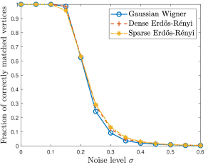
Figure 2: Universality of the performance of GRAMPA on three random graph models with 1000 vertices.

Given the latent permutation $\pi^{*}$, an edge density $p\in(0,1)$, and a noise parameter $\sigma\in[0,1]$, we generate two correlated Erdős-Rényi graphs on $n$ vertices with adjacency matrices $\mathbf{A}$ and $\mathbf{B}$, such that $(\mathbf{A}_{ij},\mathbf{B}_{\pi^{*}(i),\pi^{*}(j)})$ are i.i.d. pairs of correlated Bernoulli random variables with marginal distribution $\mathrm{Bern}(p)$. Conditional on $\mathbf{A}$,

$$\mathbf{B}_{\pi^{*}(i),\pi^{*}(j)}\sim\begin{cases}\mathrm{Bern}\big{(}1-\sigma^{2}(1-p)\big{)}&\text{ if }\mathbf{A}_{ij}=1,\\ \mathrm{Bern}\big{(}\sigma^{2}p\big{)}&\text{ if }\mathbf{A}_{ij}=0.\end{cases}$$ (72)

Here the operational meaning of the parameter $\sigma$ is that the fraction of edges which differ between the two graphs is approximately $2\sigma^{2}(1-p)\approx 2\sigma^{2}$ for sparse graphs. In particular, the extreme cases of $\sigma=0$ and $\sigma=1$ correspond to $A$ and $B$ which are perfectly correlated and independent, respectively.

Furthermore, the model parameters in (72) are calibrated to be directly comparable with the Gaussian model, so that it is convenient to verify experimentally the universality of our spectral algorithm. Indeed, denote the centered and normalized adjacency matrices by

$$A\triangleq(p(1-p)n)^{-1/2}(\mathbf{A}-\mathbb{E}[\mathbf{A}])\quad\text{ and }\quad B\triangleq(p(1-p)n)^{-1/2}(\mathbf{B}-\mathbb{E}[\mathbf{B}]).$$ (73)

Then it is easy to check that $A_{ij}$ and $B_{ij}$ both have mean zero and variance $1/n$, and moreover,

$$\mathbb{E}[(A_{ij}-B_{\pi^{*}(i),\pi^{*}(j)})^{2}]=2\sigma^{2}/n.$$ (74)

Note that equation (74) also holds for the off-diagonal entries of the Gaussian Wigner model $B=A+\sqrt{2}\sigma Z,$ where $A$ and $Z$ are independent $\mathsf{GOE}(n)$ matrices. In Figure 2, we implement GRAMPA to match pairs of Gaussian Wigner, dense Erdős-Rényi ($p=0.5$) and sparse Erdős-Rényi ($p=0.01$) graphs with 1000 vertices, and plot the fraction of correctly matched pairs of vertices against the noise level $\sigma$, averaged over 10 independent repetitions. The performance of GRAMPA on the three models is indeed similar, agreeing with the universality results proved in the companion paper [FMWX19].

For this reason, in the sequel we primarily consider the Erdős-Rényi model for synthetic experiments. In addition, while GRAMPA is applicable for matching weighted graphs, many algorithms in the literature were proposed specifically for unweighted graphs, so using the Erdős-Rényi model allows us to compare more methods in a consistent setup.

4.2 Comparison of spectral methods

We now compare the performance of GRAMPA to several existing spectral methods in the literature. Besides the rank-1 method of rounding the outer product of top eigenvectors (8) (denoted by TopEigenVec), we consider the IsoRank algorithm of [SXB08], the EigenAlign and LowRankAlign algorithms of [FQM⁺19], and Umeyama’s method [Ume88] which rounds the similarity matrix (10). In Figure 3(a), we apply these algorithms to match Erdős-Rényi graphs with $100$ vertices and edge density $0.5$. For each spectral method, we plot the fraction of correctly matched pairs of vertices of the two graphs versus the noise level $\sigma$, averaged over $10$ independent repetitions. While all estimators recover the exact matching in the noiseless case, it is clear that GRAMPA is more robust to noise than all previous spectral methods by a wide margin.

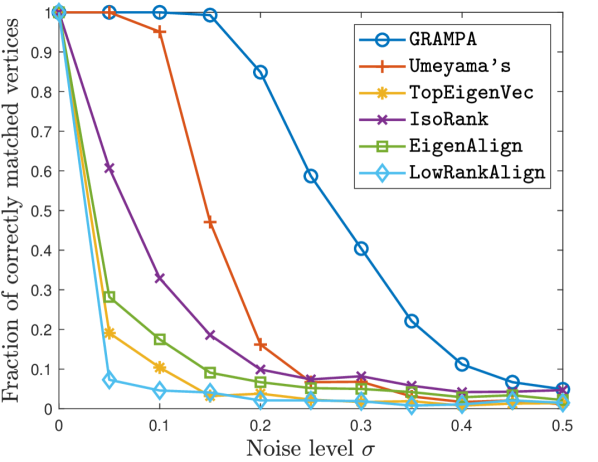
(a) Fraction of correctly matched vertices, on Erdős-Rényi graphs with $n=100$ vertices, averaged over $10$ repetitions

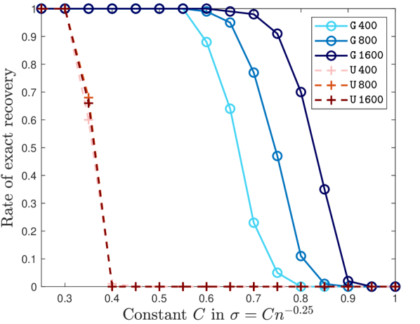
(b) Rate of exact recovery for GRAMPA and Umeyama’s method, on Erdős-Rényi graphs with a varying number of vertices, out of $100$ repetitions

Figure 3: Comparison of six spectral methods for matching Erdős-Rényi graphs with expected edge density $0.5$ and 100 vertices.

A more precise comparison of GRAMPA with its closest competitor, Umeyama’s method, is given in Fig. 3(b), which shows that Umeyama’s method is only robust to noise up to $\sigma=\frac{1}{\mathrm{poly}(n)}$, whereas we prove in [FMWX19] that GRAMPA yields exact recovery up to $\sigma=\frac{1}{\operatorname{polylog}(n)}$. Specifically, we test these two methods on Erdős-Rényi graphs with edge density $0.5$ and sizes $n=400$, $800$ and $1600$. The noise parameter $\sigma$ is set to $Cn^{-0.25}$ with varying values of $C$, where the exponent $-0.25$ is empirically found to be the critical exponent above which Umeyama’s method fails. Out of $100$ independent trials, we record the fraction of times when the algorithm exactly recovers the matching between the two graphs, and plot this quantity against $C$. From the lines U 400, U 800, and U 1600 corresponding to Umeyama’s method on the three respective graph sizes, we see that the performance of Umeyama’s method does not vary with $n$, supporting that $\sigma\asymp n^{-0.25}$ is the critical threshold for exact recovery by this method. Conversely, as $n$ increases, the failure of GRAMPA occurs at a larger value of $C$, as seen in the curves G 400, G 800, and G 1600. This aligns with the theoretical result in [FMWX19] that GRAMPA succeeds for $\sigma=\frac{1}{\operatorname{polylog}(n)}$.

4.3 Comparison with quadratic programming and Degree Profile

Next, we consider more competitive graph matching algorithms outside the spectral class. Since our method admits an interpretation through the regularized QP (15) or (16), it is of interest to compare its performance to (the algorithm that rounds the solution to) the full QP (14) with full doubly stochastic constraints, denoted by QP-DS. Another recently proposed method for graph matching is Degree Profile [DMWX18], for which theoretical guarantees comparable to our results have been established for the Gaussian Wigner and Erdős-Rényi models.

Figure 4(a) plots the fraction of correctly matched vertex pairs by the three algorithms, on Erdős-Rényi graphs with $500$ vertices and edge density $0.5$, averaged over $10$ independent repetitions. GRAMPA outperforms DegreeProfile, while QP-DS is clearly the most robust, albeit at a much higher computational cost. Since off-the-shelf QP solvers are extremely slow on instances with $n$ larger than several hundred, we resort to an alternating direction method of multipliers (ADMM) procedure used in [DMWX18]. Still, solving (14) is more than $350$ times slower than computing the similarity matrix (3) for the instances in Figure 4(a). Moreover, DegreeProfile is about $15$ times slower. We argue that GRAMPA achieves a desirable balance between speed and robustness when implemented on large networks.

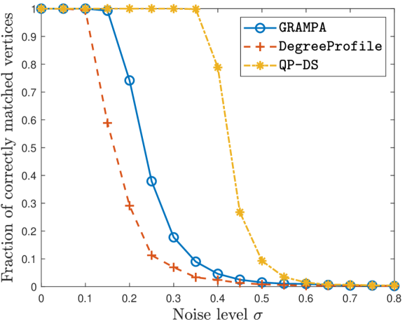
(a) Fraction of correctly matched vertices, on Erdős-Rényi graphs with $n=500$ vertices, averaged over $10$ repetitions

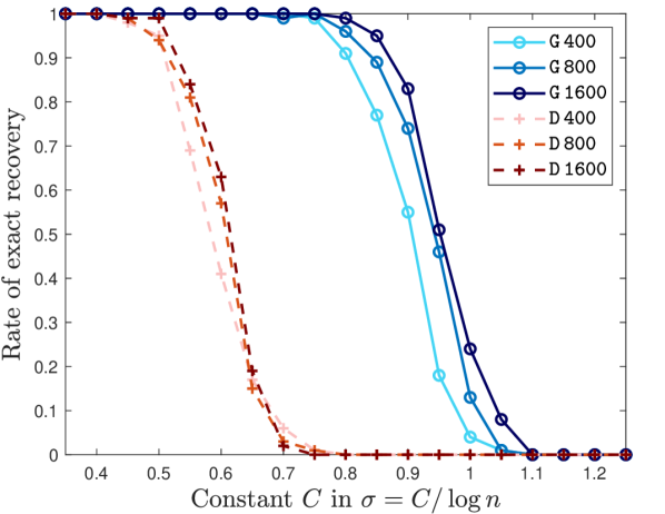
(b) Rate of exact recovery for GRAMPA and DegreeProfile, on Erdős-Rényi graphs with a varying number of vertices, out of $100$ repetitions

Figure 4: Comparison of three competitive methods for matching Erdős-Rényi graphs with expected edge density $0.5$.

A closer inspection of the exact recovery threshold of GRAMPA and DegreeProfile is done in Figure 4(b), in a similar way as Figure 3(b). Since Theorem 2.1 suggests that GRAMPA is robust to noise up to $\sigma\lesssim\frac{1}{\log n}$, we set the noise level to be $\sigma=C/\log n$, and plot the fraction of exact recovery against $C$. The results for Erdős-Rényi graphs of size $n=400,800,1600$ and for the two methods GRAMPA and DegreeProfile are represented by the curves G 400, G 800, G 1600 and D 400, D 800, D 1600 respectively. These results suggest that GRAMPA is more robust than DegreeProfile by at least a constant factor.

4.4 More graph ensembles

To demonstrate the performance of GRAMPA on other models, we turn to sparser regimes of the Erdős-Rényi model, as well as other random graph ensembles. In Figure 5, we compare the performance of GRAMPA and DegreeProfile (the two fast and robust methods from the preceding experiments) on correlated pairs of sparse Erdős-Rényi graphs, stochastic blockmodels, and power-law graphs. Following [PG11], we generate these pairs by sampling a “mother graph” according to such a model with edge density $p/s$ for $0<p<s\leq 1$, and then generating $\mathbf{A}$ and $\mathbf{B}$ by deleting each edge independently with probability $1-s$. This yields marginal edge density $p$ in both $\mathbf{A}$ and $\mathbf{B}$. We apply GRAMPA with the centered and normalized matrices $A$ and $B$ from (73) as input, with $p$ bing the marginal edge density. In each figure, the fraction of correctly matched pairs of vertices is plotted against the effective noise level

$$\sigma=\sqrt{\frac{1-s}{1-p}},$$

for graphs with $1000$ vertices, averaged over $10$ independent repetitions. One may verify that the above procedure of generating $(\mathbf{A},\mathbf{B})$ and the definition of $\sigma$ both agree with the previous definition (72) in the Erdős-Rényi setting.

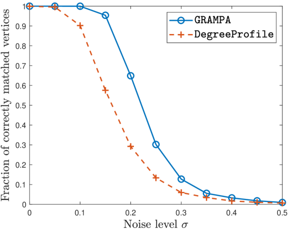
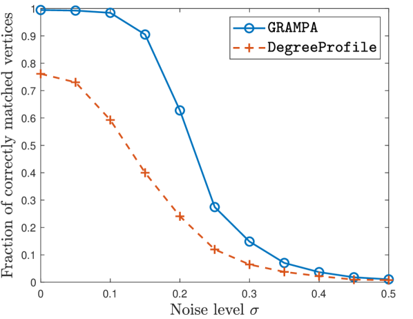
(a) Erdős-Rényi graph with
$p=0.01$

(b) Erdős-Rényi graph with
$p=0.005$

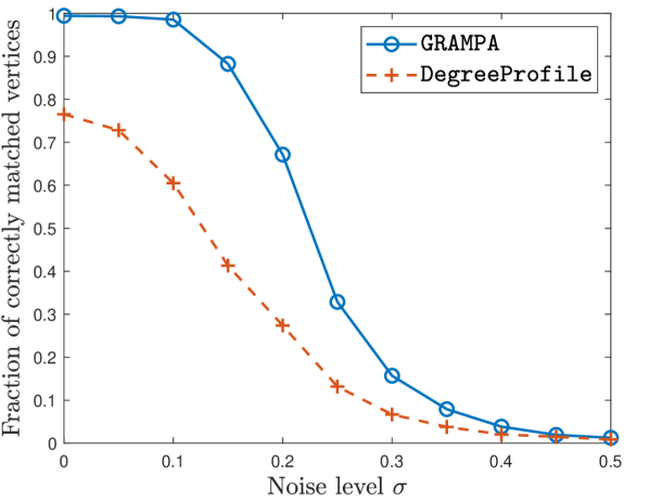
(c) Stochastic blockmodel with
$p=0.01$, $p_{\rm in}=0.016$, and $p_{\rm out}=0.004$

(d) Stochastic blockmodel with
$p=0.005$, $p_{\rm in}=0.008$, and $p_{\rm out}=0.002$

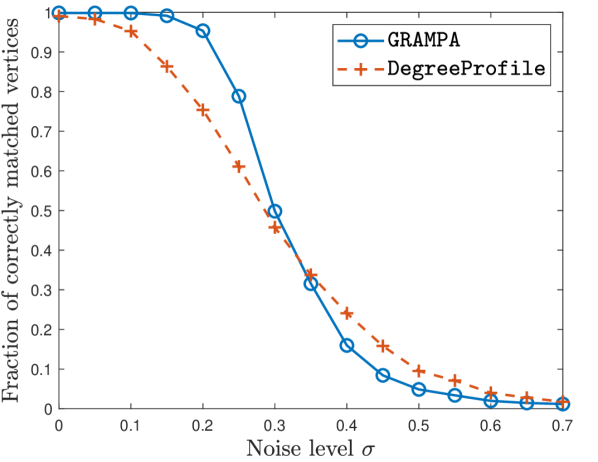
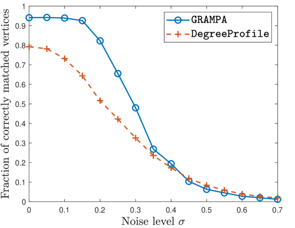
(e) Power-law graph with
$p=0.01$

(f) Power-law graph with
$p=0.005$

Figure 5: Comparison of GRAMPA and DegreeProfile on synthetic networks

In Figures 5(b) and 5(b), we consider Erdős-Rényi graphs with edge density $p=0.01$ and $0.005$. Note that the sharp threshold of $p$ for the connectedness of an Erdős-Rényi graph with $1000$ vertices is $\frac{\log n}{n}\approx 0.0069$ [ER60], below which the graphs contain isolated vertices whose matching is non-identifiable. We see that the performance of GRAMPA is better than DegreeProfile in both settings, and particularly in the sparser regime.

In Figures 5(d) and 5(d), we consider the stochastic blockmodel [HLL83] with two communities each of size $500$. The probability of an edge between vertices in the same (resp. different) community is denoted by $p_{\rm in}$ (resp. $p_{\rm out}$). The values of $p_{\rm in}$ and $p_{\rm out}$ are chosen so that the overall expected edge densities are $p=0.01$ and $0.005$ as in the Erdős-Rényi case. We observe a similar comparison of the two methods as in the Erdős-Rényi setting.

Finally, in Figures 5(f) and 5(f), we consider power-law graphs that are generated according to the following version of the Barabási-Albert preferential attachment model [BA99]: We start with two vertices connected by one edge. Then at each step, denoting the degrees of the existing $k$ vertices by $d_{1},\dots d_{k}$, we attach a new vertex to the graph by connecting it to the $j$-th existing vertex independently with probability $\max(Cd_{j}/(\sum_{i=1}^{k}d_{i}),1)$ for each $j=1,\ldots,k$. This process is iterated until the graph has $n$ vertices. Here, $C$ is a parameter that determines the final edge density.

As shown in Figure 5(f), for matching correlated power-law graphs with overall expected edge density $p=0.01$, GRAMPA is more noise resilient than DegreeProfile in terms of exact recovery. As the noise grows, the performance of GRAMPA decays faster than DegreeProfile in terms of the fraction of correctly matched pairs. In Figure 5(f), for sparser power-law graphs with expected edge density $p=0.005$, we again observe that GRAMPA has significantly better performance than DegreeProfile. Note that in this sparse regime, neither method can achieve exact recovery even in the noiseless case due to the non-trivial symmetry of the graph arising from, for example, multiple leaf vertices incident to a common parent. We revisit the issue of non-identifiability when studying the real dataset in the next subsection.

4.5 Networks of autonomous systems

We corroborate the improvement of GRAMPA over DegreeProfile using quantitative benchmarks on a time-evolving real-world network of $n=10000$ vertices. Here, for simplicity, we apply both methods to the unnormalized adjacency matrices, and set $\eta=1$ for GRAMPA. We find that the results are not very sensitive to this choice of $\eta$. Although QP-DS yields better performance in Fig. 4, it is extremely slow to run on such a large network, so we omit it from the comparison here.

We use a subset of the Autonomous Systems dataset from the University of Oregon Route Views Project [Uni], available as part of the Stanford Network Analysis Project [LK14, LKF05]. The data consists of instances of a network of autonomous systems observed on nine days between March 31, 2001 and May 26, 2001. Edges and (a small fraction of) vertices of the network were added and deleted over time. In particular, the number of vertices of the network on the nine days ranges from 10,670 to 11,174 and the number of edges from 22,002 to 23,409. The labels of the vertices are known.

To test the graph matching methods, we consider 10,000 vertices of the network that are present on all nine days. The resulting nine graphs can be seen as noisy versions of each other, with correlation decaying over time. We apply GRAMPA and DegreeProfile to match each graph to that on the first day of March 31, with vertices randomly permuted.

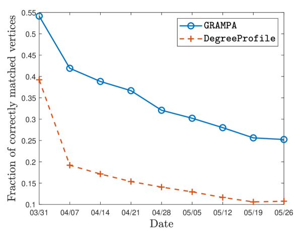
(a) Fraction of correctly matched vertices

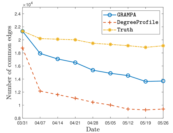
(b) Number of common edges

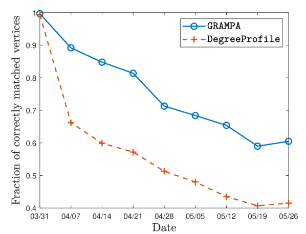
(c) Fraction of correctly matched vertices, in high-degree subgraph of 1000 vertices

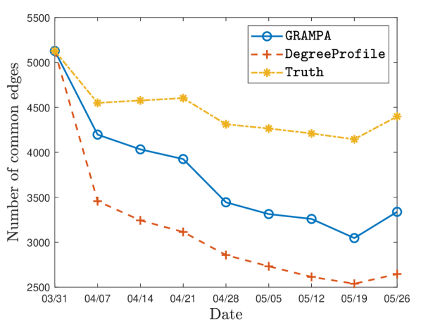
(d) Number of common edges, in high-degree subgraph of 1000 vertices

Figure 6: Comparison of GRAMPA and DegreeProfile for matching networks of autonomous systems on nine days to that on the first day

In Figure 6(a), we plot the fraction of correctly matched pairs of vertices against the chronologically ordered dates. GRAMPA correctly matches many more pairs of vertices than DegreeProfile for all nine days. As expected, the performance of both methods degrades over time as the network becomes less correlated with the original one.

For the same reason as in the power-law graphs in Fig. 5(f), even the matching of the graph on the first day to itself is not exact. In fact, there are over 3,000 degree-one vertices in this graph, and some of them are attached to the same high-degree vertices, so the exact matching is non-identifiable. Thus for a given matching $\widehat{\pi}$, an arguably more relevant figure of merit is the number of common edges, i.e. the (rescaled) objective value $\langle A,B^{\widehat{\pi}}\rangle/2$. We plot this in Figure 6(b) together with the value for the ground-truth matching. The values of GRAMPA and of the ground-truth matching are the same on the first day, indicating that GRAMPA successfully finds an automorphism of this graph, while DegreeProfile fails. Furthermore, GRAMPA consistently recovers a matching with more common edges over the nine days.

As in many real-world networks, high-degree vertices here are hubs in the network of autonomous systems and play a more important role. Therefore, we further evaluate the two methods by comparing their performance on subgraphs induced by high-degree vertices. More precisely, we consider the 1,000 vertices that have the highest degrees in the graph on the first day, March 31. In Figures 6(c) and 6(d), we still use the matchings between the entire networks that generated Figures 6(a) and 6(b), but evaluate the correctness only on those top 1,000 high-degree vertices. We observe that both methods succeed in exactly matching the subgraph from the first day to itself, and in general yield much better matchings for the high-degree vertices than for the remainder of the graph. Again, GRAMPA produces better results than DegreeProfile on these subgraphs over the nine days, in both measures of performance.

5 Conclusion

We have proposed a highly practical spectral method, GRAMPA, for matching a pair of edge-correlated graphs. By using a similarity matrix that is a weighted combination of outer products $u_{i}v_{j}^{\top}$ across all pairs of eigenvectors of the two adjacency matrices, GRAMPA exhibits significantly improved noise resilience over previous spectral approaches. We showed in this work that GRAMPA achieves exact recovery of the latent matching in a correlated Gaussian Wigner model, up to a noise level $\sigma\lesssim\frac{1}{\log n}$. In the companion paper [FMWX19], we establish a similar universal guarantee for Erdős-Rényi graphs and other correlated Wigner matrices, up to a noise level $\sigma\lesssim\frac{1}{\operatorname{polylog}n}$. GRAMPA exhibits improved recovery accuracy over previous spectral methods as well as the state-of-the-art degree profile algorithm in [DMWX18], on a variety of synthetic graphs and also on a real network example.

The similarity matrix (3) in GRAMPA can be interpreted as a ridge-regularized further relaxation of the well-known quadratic relaxation (14) of the QAP, where the doubly-stochastic constraint is replaced by $\mathbf{1}^{\top}X\mathbf{1}=n$. In the companion paper [FMWX19], we also analyze a tighter relaxation with constraints $X\mathbf{1}=\mathbf{1}$, and establish similar guarantees. In synthetic experiments on small graphs, we found that solving the full quadratic program (14), followed by the same rounding procedure as used in GRAMPA, yields better recovery accuracy in noisy settings. However, unlike GRAMPA, solving (14) does not scale to large networks, and the properties of its solution currently lack theoretical understanding. We leave these as open problems for future work.

Appendix A Concentration inequalities for Gaussians

We collect auxiliary results on concentration of polynomials of Gaussian variables.

Lemma A.1.

Let $z$ be a standard Gaussian vector in $\mathbb{R}^{n}$. For any fixed $v\in\mathbb{R}^{n}$ and $\delta>0$, it holds with probability at least $1-\delta$ that

$$|v^{\top}z|\leq\|v\|_{2}\sqrt{2\log(1/\delta)}.$$

Lemma A.2 (Hanson-Wright inequality).

Let $z$ be a sub-Gaussian vector in $\mathbb{R}^{n}$, and let $M$ be a fixed matrix in ${\mathbb{C}}^{n\times n}$. Then we have with probability at least $1-\delta$ that

$$|z^{\top}Mz-\operatorname{Tr}M| \leq C\|z\|_{\psi_{2}}^{2}\Big{(}\|M\|_{F}\sqrt{\log(1/\delta)}+\|M\|\log(1/\delta)\Big{)}$$ (75)

$$\leq 2C\|z\|_{\psi_{2}}^{2}\|M\|_{F}\log(1/\delta),$$

where $C$ is a universal constant and $\|z\|_{\psi_{2}}$ is the sub-Gaussian norm of $z$.

See [RV13, Section 3.1] for the complex-valued version of the Hanson-Wright inequality. The following lemma is a direct consequence of (75), by taking $M$ to be a diagonal matrix.

Lemma A.3.

Let $z$ be a standard Gaussian vector in $\mathbb{R}^{n}$. For an entrywise nonnegative vector $v\in\mathbb{R}^{n}$, it holds with probability at least $1-\delta$ that

$$\Big{|}\sum_{i=1}^{n}v_{i}z_{i}^{2}-\sum_{i=1}^{n}v_{i}\Big{|}\leq C\Big{(}\|v\|_{2}\sqrt{\log(1/\delta)}+\|v\|_{\infty}\log(1/\delta)\Big{)}.$$

In particular, it holds with probability at least $1-\delta$ that

$$\big{|}\|z\|_{2}^{2}-n\big{|}\leq C\Big{(}\sqrt{n\log(1/\delta)}+\log(1/\delta)\Big{)}.$$

Theorem A.4 (Hypercontractivity concentration [SS12, Theorem 1.9]).

Let $z$ be a standard Gaussian vector in $\mathbb{R}^{n}$, and let $f(z_{1},\dots,z_{n})$ be a degree-$d$ polynomial of $z$. Then it holds that

$$\mathbb{P}\Big{\{}\big{|}f(z)-\mathbb{E}[f(z)]\big{|}>t\Big{\}}\leq e^{2}\exp\bigg{[}-\Big{(}\frac{t^{2}}{C\,\mathsf{Var}[f(z)]}\Big{)}^{1/d}\bigg{]},$$

where $\mathsf{Var}[f(z)]$ denotes the variance of $f(z)$ and $C>0$ is a universal constant.

Finally, the following result gives a concentration inequality in terms of the restricted Lipschitz constants, obtained from the usual Gaussian concentration of measure plus a Lipschitz extension argument.

Lemma A.5.

Let $B\subset{\mathbb{R}}^{n}$ be an arbitrary measurable subset. Let $F:{\mathbb{R}}^{n}\to{\mathbb{R}}$ such that $F$ is $L$-Lipschitz on $B$. Let $X\sim N(0,\mathbf{I}_{n})$. Then for any $t>0$,

$$\mathbb{P}\left\{|F(X)-\mathbb{E}F(X)|\geq t+\delta\right\}\leq\exp\left(-\frac{ct^{2}}{L^{2}}\right)+\epsilon,$$

where $c$ is a universal constant, $\epsilon=\mathbb{P}\left\{X\notin B\right\}$ and $\delta=2\sqrt{\epsilon(nL^{2}+F(0)^{2}+\mathbb{E}[F(X)^{2}])}$.

Proof.

Let $\widetilde{F}:{\mathbb{R}}^{n}\to{\mathbb{R}}$ be an $L$-Lipschitz extension of $F$, e.g., $\widetilde{F}(x)=\inf_{y\in B}F(y)+L\|x-y\|$. Then by the Gaussian concentration inequality (cf. e.g. [Ver18, Theorem 5.2.2]), we have

$$\mathbb{P}\left\{|\widetilde{F}(X)-\mathbb{E}\widetilde{F}(X)|\geq t\right\}\leq\exp\left(-\frac{ct^{2}}{L^{2}}\right).$$

It remains to show that $|\mathbb{E}F(X)-\mathbb{E}\widetilde{F}(X)|\leq\delta$. Indeed, by Cauchy-Schwarz, $|\mathbb{E}F(X)-\mathbb{E}\widetilde{F}(X)|\leq\mathbb{E}|F(X-\widetilde{F}(X)|{\mathbf{1}_{\left\{{X\notin B}\right\}}}\leq\sqrt{\epsilon\mathbb{E}[|F(X-\widetilde{F}(X)|^{2}]}$. Finally, noting that $|\widetilde{F}(X)|\leq F(0)+L\|X\|_{2}$ and $\mathbb{E}\|X\|_{2}^{2}=n$ completes the proof. ∎

Appendix B Kronecker gymnastics

Given $A,B\in{\mathbb{C}}^{n\times n}$, the Kronecker product $A\otimes B\in{\mathbb{C}}^{n^{2}\times n^{2}}$ is defined as $\left[\begin{smallmatrix}a_{11}B&\ldots&a_{1n}B\\ \vdots&\vdots&\vdots\\ a_{n1}B&\ldots&a_{nn}B\end{smallmatrix}\right]$. The vectorized form of $A=[a_{1},\ldots,a_{n}]$ is $\mathsf{vec}(A)=[a_{1}^{\top},\ldots,a_{n}^{\top}]^{\top}\in{\mathbb{C}}^{n\otimes n}$. It is convenient to identify $[n^{2}]$ with by $[n]^{2}$ ordered as $\{(1,1),\ldots,(1,n),\ldots,(n,n)\}$, in which case we have $(A\otimes B)_{ij,k\ell}=A_{ik}B_{j\ell}$ and $\mathsf{vec}(A)_{ij}=A_{ij}$.

We collect some identities for Kronecker products and vectorizations of matrices used throughout this paper:

$$\langle A\otimes A,B\otimes B\rangle =\langle A,B\rangle^{2},$$

$$(A\otimes B)(U\otimes V) =AU\otimes BV,$$

$$\mathsf{vec}(AUB) =(B^{\top}\otimes A)\mathsf{vec}(U),$$

$$(X\otimes Y)\mathsf{vec}(U) =\mathsf{vec}(YUX^{\top}),$$

$$(A\otimes B)^{\top} =A^{\top}\otimes B^{\top}.$$

The third equality implies that

$$\langle A\otimes B,\mathsf{vec}(U)\mathsf{vec}(V)^{\top}\rangle =\langle\mathsf{vec}(U),(A\otimes B)\mathsf{vec}(V)\rangle$$

$$=\langle\mathsf{vec}(U),\mathsf{vec}(BVA^{\top})\rangle=\langle U,BVA^{\top}\rangle=\langle B,UAV^{\top}\rangle$$

and hence

$$\mathsf{vec}(U)^{\top}(A\otimes B)\mathsf{vec}(V)=\langle A\otimes B,\mathsf{vec}(U)\mathsf{vec}(V)^{\top}\rangle =\langle B,UAV^{\top}\rangle=\langle A,U^{\top}BV\rangle=\langle UA,BV\rangle.$$

Applying the third equality to column vector $z$ and noting that $\mathsf{vec}(z^{\top})=\mathsf{vec}(z)=z$, we have

$$(X\otimes y)z= ~{}\mathsf{vec}(yz^{\top}X^{\top}),$$

$$(y\otimes X)z= ~{}\mathsf{vec}(Xzy^{\top}).$$

In particular, it holds that

$$(\mathbf{I}\otimes y)z= ~{}\mathsf{vec}(yz^{\top})=z\otimes y,$$

$$(y\otimes\mathbf{I})z= ~{}\mathsf{vec}(zy^{\top})=y\otimes z.$$

Appendix C Signal-to-noise heuristics

We justify the choice of the Cauchy weight kernel in (4) by a heuristic signal-to-noise calculation for $\widehat{X}$. We assume without loss of generality that $\pi^{*}$ is the identity, so that diagonal entries of $\widehat{X}$ indicate similarity between matching vertices of $A$ and $B$. Then for the rounding procedure in (5), we may interpret $n^{-1}\operatorname{Tr}\widehat{X}$ and $(n^{-2}\sum_{i,j:\,i\neq j}\widehat{X}_{ij}^{2})^{1/2}\approx n^{-1}\|\widehat{X}\|_{F}$ as the average signal strength and noise level in $\widehat{X}$. Let us define a corresponding signal-to-noise ratio as

$$\mathrm{SNR}=\frac{\mathbb{E}[\operatorname{Tr}\widehat{X}]}{\mathbb{E}[\|\widehat{X}\|_{F}^{2}]^{1/2}}$$

and compute this quantity in the Gaussian Wigner model.

We abbreviate the spectral weights $w(\lambda_{i},\mu_{j})$ as $w_{ij}$. For $\widehat{X}$ defined by (3) with any weight kernel $w(x,y)$, we have

$$\operatorname{Tr}\widehat{X}=\sum_{ij}w_{ij}\cdot u_{i}^{\top}\mathbf{J}v_{j}\cdot u_{i}^{\top}v_{j}.$$

Applying that $(A,B)$ is equal in law to $(OAO^{\top},OBO^{\top})$ for a rotation $O$ such that $O\mathbf{1}=\sqrt{n}\mathbf{e}_{k}$, we obtain for every $k$ that

$$\mathbb{E}[\operatorname{Tr}\widehat{X}]=\sum_{ij}n\cdot\mathbb{E}[w_{ij}\cdot u_{i}^{\top}(\mathbf{e}_{k}\mathbf{e}_{k}^{\top})v_{j}\cdot u_{i}^{\top}v_{j}].$$

Then averaging over $k=1,\ldots,n$ and applying $\sum_{k}\mathbf{e}_{k}\mathbf{e}_{k}^{\top}=\mathbf{I}$ yield that

$$\mathbb{E}[\operatorname{Tr}\widehat{X}]=\sum_{ij}\mathbb{E}[w_{ij}(u_{i}^{\top}v_{j})^{2}].$$

For the noise, we have

$$\|\widehat{X}\|_{F}^{2}=\operatorname{Tr}\widehat{X}\widehat{X}^{\top}=\sum_{i,j,k,l}w_{ij}w_{kl}(u_{i}^{\top}\mathbf{J}v_{j})(u_{k}^{\top}\mathbf{J}v_{\ell})\operatorname{Tr}(u_{i}v_{j}^{\top}\cdot v_{\ell}u_{k}^{\top})=\sum_{ij}w_{ij}^{2}(u_{i}^{\top}\mathbf{J}v_{j})^{2}.$$

Applying the equality in law of $(A,B)$ and $(OAO^{\top},OBO^{\top})$ for a uniform random orthogonal matrix $O$, and writing $r=O\mathbf{1}/\sqrt{n}$, we get

$$\mathbb{E}[\|\widehat{X}\|_{F}^{2}]=\sum_{ij}n^{2}\cdot\mathbb{E}[w_{ij}^{2}(u_{i}^{\top}r)^{2}(v_{j}^{\top}r)^{2}].$$

Here, $r=(r_{1},\ldots,r_{n})$ is a uniform random vector on the unit sphere, independent of $(A,B)$. For any deterministic unit vectors $u,v$ with $u^{\top}v=\alpha$, we may rotate to $u=\mathbf{e}_{1}$ and $v=\alpha\mathbf{e}_{1}+\sqrt{1-\alpha^{2}}\mathbf{e}_{2}$ to get

$$\mathbb{E}[(u^{\top}r)^{2}(v^{\top}r)^{2}]=\mathbb{E}[r_{1}^{2}\cdot(\alpha r_{1}+\sqrt{1-\alpha^{2}}r_{2})^{2}]=\alpha^{2}\mathbb{E}[r_{1}^{4}]+(1-\alpha^{2})\mathbb{E}[r_{1}^{2}r_{2}^{2}]=\frac{1+2\alpha^{2}}{n(n+2)},$$

where the last equality applies an elementary computation. Bounding $1+2\alpha^{2}\in[1,3]$ and applying this conditional on $(A,B)$ above, we obtain

$$\mathbb{E}[\|\widehat{X}\|_{F}^{2}]=\frac{cn}{n+2}\sum_{ij}\mathbb{E}[w_{ij}^{2}]$$

for some value $c\in[1,3]$.

To summarize,

$$\mathrm{SNR}\asymp\frac{\sum_{ij}\mathbb{E}[w(\lambda_{i},\mu_{j})(u_{i}^{\top}v_{j})^{2}]}{\sqrt{\sum_{ij}\mathbb{E}[w(\lambda_{i},\mu_{j})^{2}]}}.$$

The choice of weights which maximizes this SNR would satisfy $w(\lambda_{i},\mu_{j})\propto(u_{i}^{\top}v_{j})^{2}$. Recall that for $n^{-1+\varepsilon}\ll\sigma^{2}\ll n^{-\varepsilon}$ and $i,j$ in the bulk of the spectrum, we have the approximation (11). Thus this optimal choice of weights takes a Cauchy form, which motivates our choice in (4).

We note that this discussion is only heuristic, and maximizing this definition of SNR does not automatically imply any rigorous guarantee for exact recovery of $\pi^{*}$. Our proposal in (4) is a bit simpler than the optimal choice suggested by (11): The constant $C$ in (11) depends on the semicircle density near $\lambda_{i}$, but we do not incorporate this dependence in our definition. Also, while (11) depends on the noise level $\sigma$, our main result in Theorem 2.1 shows that $\eta$ need not be set based on $\sigma$, which is usually unknown in practice. Instead, our result shows that the simpler choice $\eta=c/\log n$ is sufficient for exact recovery of $\pi^{*}$ over a range of noise levels $\sigma\lesssim\eta$.

References

- [ABK15] Yonathan Aflalo, Alexander Bronstein, and Ron Kimmel. On convex relaxation of graph isomorphism. Proceedings of the National Academy of Sciences, 112(10):2942–2947, 2015.
- [AD93] HA Almohamad and Salih O Duffuaa. A linear programming approach for the weighted graph matching problem. IEEE Transactions on pattern analysis and machine intelligence, 15(5):522–525, 1993.
- [AGZ10] Greg W Anderson, Alice Guionnet, and Ofer Zeitouni. An introduction to random matrices, volume 118. Cambridge university press, 2010.
- [BA99] Albert-László Barabási and Réka Albert. Emergence of scaling in random networks. Science, 286(5439):509–512, 1999.
- [BCL+18] Boaz Barak, Chi-Ning Chou, Zhixian Lei, Tselil Schramm, and Yueqi Sheng. (Nearly) efficient algorithms for the graph matching problem on correlated random graphs. arXiv preprint arXiv:1805.02349, 2018.
- [BCPP98] Rainer E Burkard, Eranda Cela, Panos M Pardalos, and Leonidas S Pitsoulis. The quadratic assignment problem. In Handbook of combinatorial optimization, pages 1713–1809. Springer, 1998.
- [Ben17] Lucas Benigni. Eigenvectors distribution and quantum unique ergodicity for deformed Wigner matrices. arXiv preprint arXiv:1711.07103, 2017.
- [BGM82] László Babai, D Yu Grigoryev, and David M Mount. Isomorphism of graphs with bounded eigenvalue multiplicity. In Proceedings of the fourteenth annual ACM symposium on Theory of computing, pages 310–324. ACM, 1982.
- [Bol82] Béla Bollobás. Distinguishing vertices of random graphs. North-Holland Mathematics Studies, 62:33–49, 1982.
- [BY17] Paul Bourgade and H-T Yau. The eigenvector moment flow and local quantum unique ergodicity. Communications in Mathematical Physics, 350(1):231–278, 2017.
- [CFSV04] Donatello Conte, Pasquale Foggia, Carlo Sansone, and Mario Vento. Thirty years of graph matching in pattern recognition. International journal of pattern recognition and artificial intelligence, 18(03):265–298, 2004.
- [Cha14] Sourav Chatterjee. Superconcentration and related topics, volume 15. Springer, 2014.
- [CK16] Daniel Cullina and Negar Kiyavash. Improved achievability and converse bounds for Erdös-Rényi graph matching. In Proceedings of the 2016 ACM SIGMETRICS International Conference on Measurement and Modeling of Computer Science, pages 63–72. ACM, 2016.
- [CK17] Daniel Cullina and Negar Kiyavash. Exact alignment recovery for correlated Erdös-Rényi graphs. arXiv preprint arXiv:1711.06783, 2017.
- [CKMP18] Daniel Cullina, Negar Kiyavash, Prateek Mittal, and H Vincent Poor. Partial recovery of Erdős-Rényi graph alignment via -core alignment. arXiv preprint arXiv:1809.03553, Nov. 2018.
- [CP08] Tomek Czajka and Gopal Pandurangan. Improved random graph isomorphism. Journal of Discrete Algorithms, 6(1):85–92, 2008.
- [DCK19] Osman Emre Dai, Daniel Cullina, and Negar Kiyavash. Database alignment with gaussian features. arXiv preprint arXiv:1903.01422, 2019.
- [DCKG18] Osman Emre Dai, Daniel Cullina, Negar Kiyavash, and Matthias Grossglauser. On the performance of a canonical labeling for matching correlated Erdős-Rényi graphs. arXiv preprint arXiv:1804.09758, 2018.
- [DML17] Nadav Dym, Haggai Maron, and Yaron Lipman. DS++: a flexible, scalable and provably tight relaxation for matching problems. ACM Transactions on Graphics (TOG), 36(6):184, 2017.
- [DMWX18] Jian Ding, Zongming Ma, Yihong Wu, and Jiaming Xu. Efficient random graph matching via degree profiles. arxiv preprint arxiv:1811.07821, Nov 2018.
- [ER60] P. Erdös and A. Rényi. On the evolution of random graphs. Publ. Math. Inst. Hungar. Acad. Sci, 5:17–61, 1960.
- [ESDS16] Frank Emmert-Streib, Matthias Dehmer, and Yongtang Shi. Fifty years of graph matching, network alignment and network comparison. Information Sciences, 346:180–197, 2016.
- [FBR87] Gerd Finke, Rainer E Burkard, and Franz Rendl. Quadratic assignment problems. In North-Holland Mathematics Studies, volume 132, pages 61–82. Elsevier, 1987.
- [FJBd13] Fajwel Fogel, Rodolphe Jenatton, Francis Bach, and Alexandre d’Aspremont. Convex relaxations for permutation problems. In Advances in Neural Information Processing Systems, pages 1016–1024, 2013.
- [FMWX19] Zhou Fan, Cheng Mao, Yihong Wu, and Jiaming Xu. Spectral graph matching and regularized quadratic relaxations II: Erdős-Rényi graphs and universality. preprint, 2019.
- [FQM+19] Soheil Feizi, Gerald Quon, Mariana Mendoza, Muriel Medard, Manolis Kellis, and Ali Jadbabaie. Spectral alignment of graphs. IEEE Transactions on Network Science and Engineering, 2019.
- [FQRM+16] Soheil Feizi, Gerald Quon, Mariana Recamonde-Mendoza, Muriel Médard, Manolis Kellis, and Ali Jadbabaie. Spectral alignment of networks. arXiv preprint arXiv:1602.04181, 2016.
- [GT11] Friedrich Götze and A Tikhomirov. On the rate of convergence to the marchenko–pastur distribution. arXiv preprint arXiv:1110.1284, 2011.
- [GT13] Friedrich Götze and Alexandre Tikhomirov. On the rate of convergence to the semi-circular law. In High Dimensional Probability VI, pages 139–165, Basel, 2013. Springer Basel.
- [HLL83] P. W. Holland, K. B. Laskey, and S. Leinhardt. Stochastic blockmodels: First steps. Social Networks, 5(2):109–137, 1983.
- [Kat73] Tosio Kato. Continuity of the map for linear operators. Proceedings of the Japan Academy, 49(3):157–160, 1973.
- [KG16] Ehsan Kazemi and Matthias Grossglauser. On the structure and efficient computation of isorank node similarities. arXiv preprint arXiv:1602.00668, 2016.
- [KHG15] Ehsan Kazemi, S Hamed Hassani, and Matthias Grossglauser. Growing a graph matching from a handful of seeds. Proceedings of the VLDB Endowment, 8(10):1010–1021, 2015.
- [KHGM16] Ehsan Kazemi, Hamed Hassani, Matthias Grossglauser, and Hassan Pezeshgi Modarres. Proper: global protein interaction network alignment through percolation matching. BMC bioinformatics, 17(1):527, 2016.
- [KL14] Nitish Korula and Silvio Lattanzi. An efficient reconciliation algorithm for social networks. Proceedings of the VLDB Endowment, 7(5):377–388, 2014.
- [Kuh55] Harold W Kuhn. The Hungarian method for the assignment problem. Naval research logistics quarterly, 2(1-2):83–97, 1955.
- [LFF+16] Vince Lyzinski, Donniell Fishkind, Marcelo Fiori, Joshua Vogelstein, Carey Priebe, and Guillermo Sapiro. Graph matching: Relax at your own risk. IEEE Transactions on Pattern Analysis & Machine Intelligence, 38(1):60–73, 2016.
- [LFP14] Vince Lyzinski, Donniell E Fishkind, and Carey E Priebe. Seeded graph matching for correlated Erdös-Rényi graphs. Journal of Machine Learning Research, 15(1):3513–3540, 2014.
- [LK14] Jure Leskovec and Andrej Krevl. SNAP Datasets: Stanford large network dataset collection. http://snap.stanford.edu/data, June 2014.
- [LKF05] Jure Leskovec, Jon Kleinberg, and Christos Faloutsos. Graphs over time: densification laws, shrinking diameters and possible explanations. In Proceedings of the eleventh ACM SIGKDD international conference on Knowledge discovery in data mining, pages 177–187. ACM, 2005.
- [LR13] Lorenzo Livi and Antonello Rizzi. The graph matching problem. Pattern Analysis and Applications, 16(3):253–283, 2013.
- [LS18] Joseph Lubars and R Srikant. Correcting the output of approximate graph matching algorithms. In IEEE INFOCOM 2018-IEEE Conference on Computer Communications, pages 1745–1753. IEEE, 2018.
- [MMS10] Konstantin Makarychev, Rajsekar Manokaran, and Maxim Sviridenko. Maximum quadratic assignment problem: Reduction from maximum label cover and LP-based approximation algorithm. Automata, Languages and Programming, pages 594–604, 2010.
- [MX19] Elchanan Mossel and Jiaming Xu. Seeded graph matching via large neighborhood statistics. In Proceedings of the Thirtieth Annual ACM-SIAM Symposium on Discrete Algorithms, pages 1005–1014. SIAM, 2019.
- [NS08] Arvind Narayanan and Vitaly Shmatikov. Robust de-anonymization of large sparse datasets. In Security and Privacy, 2008. SP 2008. IEEE Symposium on, pages 111–125. IEEE, 2008.
- [NS09] Arvind Narayanan and Vitaly Shmatikov. De-anonymizing social networks. In Security and Privacy, 2009 30th IEEE Symposium on, pages 173–187. IEEE, 2009.
- [PG11] Pedram Pedarsani and Matthias Grossglauser. On the privacy of anonymized networks. In ACM SIGKDD International Conference on Knowledge Discovery and Data Mining, pages 1235–1243, 2011.
- [PRW94] Panos M. Pardalos, Franz Rendl, and Henry Wolkowicz. The quadratic assignment problem: A survey and recent developments. In In Proceedings of the DIMACS Workshop on Quadratic Assignment Problems, volume 16 of DIMACS Series in Discrete Mathematics and Theoretical Computer Science, pages 1–42. American Mathematical Society, 1994.
- [RV13] Mark Rudelson and Roman Vershynin. Hanson-Wright inequality and sub-Gaussian concentration. Electron. Commun. Probab., 18:no. 82, 9, 2013.
- [SGE17] Farhad Shirani, Siddharth Garg, and Elza Erkip. Seeded graph matching: Efficient algorithms and theoretical guarantees. In 2017 51st Asilomar Conference on Signals, Systems, and Computers, pages 253–257. IEEE, 2017.
- [SS05] Christian Schellewald and Christoph Schnörr. Probabilistic subgraph matching based on convex relaxation. In International Workshop on Energy Minimization Methods in Computer Vision and Pattern Recognition, pages 171–186. Springer, 2005.
- [SS12] Warren Schudy and Maxim Sviridenko. Concentration and moment inequalities for polynomials of independent random variables. In Proceedings of the Twenty-Third Annual ACM-SIAM Symposium on Discrete Algorithms, pages 437–446. ACM, New York, 2012.
- [SXB08] Rohit Singh, Jinbo Xu, and Bonnie Berger. Global alignment of multiple protein interaction networks with application to functional orthology detection. Proceedings of the National Academy of Sciences, 105(35):12763–12768, 2008.
- [Ume88] Shinji Umeyama. An eigendecomposition approach to weighted graph matching problems. IEEE transactions on pattern analysis and machine intelligence, 10(5):695–703, 1988.
- [Uni] University of Oregon Route Views Project. Autonomous Systems Peering Networks. Online data and reports, http://www.routeviews.org/.
- [VCL+15] Joshua T Vogelstein, John M Conroy, Vince Lyzinski, Louis J Podrazik, Steven G Kratzer, Eric T Harley, Donniell E Fishkind, R Jacob Vogelstein, and Carey E Priebe. Fast approximate quadratic programming for graph matching. PLOS one, 10(4):e0121002, 2015.
- [Ver18] Roman Vershynin. High-Dimensional Probability: An Introduction with Applications in Data Science. Cambridge Series in Statistical and Probabilistic Mathematics. Cambridge University Press, 2018.
- [XK01] Lei Xu and Irwin King. A PCA approach for fast retrieval of structural patterns in attributed graphs. IEEE Transactions on Systems, Man, and Cybernetics, Part B (Cybernetics), 31(5):812–817, 2001.
- [YG13] Lyudmila Yartseva and Matthias Grossglauser. On the performance of percolation graph matching. In Proceedings of the first ACM conference on Online social networks, pages 119–130. ACM, 2013.
- [ZBV08] Mikhail Zaslavskiy, Francis Bach, and Jean-Philippe Vert. A path following algorithm for the graph matching problem. IEEE Transactions on Pattern Analysis and Machine Intelligence, 31(12):2227–2242, 2008.