Occupation densities of Ensembles of Branching Random Walks

Abstract.

We study the limiting occupation density process for a large number of critical and driftless branching random walks. We show that the rescaled occupation densities of $\lfloor sN\rfloor$ branching random walks, viewed as a function-valued, increasing process $\{g_{s}^{N}\}_{s\geq 0}$, converges weakly to a pure jump process in the Skorohod space $\mathbb{D}([0,+\infty),\mathcal{C}_{0}(\mathbb{R}))$, as $N\to\infty$. Moreover, the jumps of the limiting process consist of i.i.d. copies of an Integrated super-Brownian Excursion (ISE) density, rescaled and weighted by the jump sizes in a real-valued stable-1/2 subordinator.

1. Introduction

In a branching random walk on the integers, individuals live for one generation, reproduce as in a Galton-Watson process, giving rise to offspring which then independently jump according to the law of a random walk. A branching random walk is said to be critical if the offspring distribution $\nu$ has mean $1$, and driftless if the jump distribution $F$ has mean $0$ and finite variance. We will assume throughout that (i) the offspring distribution $\nu$ has mean one (so that the Galton-Watson process is critical) and finite, positive variance $\sigma^{2}_{\nu}$; and (ii) the step distribution $F$ for the random walk has span one, mean zero and finite, positive variance $\sigma^{2}_{F}$. (Thus, the spatial locations of individuals will always be points of the integers $\mathbb{Z}$.)

To any branching random walk can be associated a randomly labeled Galton-Watson tree $\mathcal{T}$, where the Galton-Watson tree describes the lineage of the individuals and the label of each vertex marks the spatial location of the corresponding individual. This labeled tree

$$\mathcal{T}=(T,\{l(v)\}_{v\in T})$$

is generated as follows.

1. Let $T$ be the genealogical tree of a Galton-Watson process with a single ancestral individual and offspring distribution $\nu$, with the root node $\rho$ representing this ancestral individual. Since $\nu$ has mean $1$, the tree $T$ is finite with probability one.

2. Assign the label $l(\rho)=0$ to the root.

3. Conditional on $T$, let $\left\{\xi_{e}\right\}_{e\in\mathcal{E}(T)}$ be a collection of i.i.d. random variables, with common distribution $F$ (the “step distribution”) indexed by the (directed) edges $e=(u,v)$ of the tree $T$, where $u$ is the parent vertex of $v$. For any such directed edge $e=(u,v)$, define

   $$l(v)=l(u)+\xi_{e}.$$

Given the labeled tree $\mathcal{T}$ associated with the branching random walk, the occupation measures can be recovered as follows. For any time $n\in\mathbb{Z}_{+}$ and any site $x\in\mathbb{Z}$, the number $Z_{n}(x)$ of individuals at location $x$ at time $n$ is the number of vertices $v\in T$ at height $n$ (i.e., at distance $n$ from the root) with label $l(v)=x$. The vertical profile, or the occupation measure, of $\mathcal{T}$ (see [5]) is the random counting measure on $\mathbb{Z}$ defined by

$$X(x;\mathcal{T})=\sum_{n=0}^{\infty}Z_{n}(x).$$

In this paper, we study the limiting behavior of the occupation measure and its connection to super-Brownian motions. Before stating our main result, we review a few results about the occupation measure of random labeled trees.

The study of such occupation measures dates back to Aldous [3], who introduced an object called the integrated super-Brownian excursion (ISE), denoted by $\mu_{\textup{ISE}}$, a (probability) measure-valued random variable that arises as the scaling limit of the occupation measure of certain labeled random planar trees and tree embeddings. In [12], Marckert proved that the rescaled occupation measure of a random binary tree of $n$ vertices converges weakly to $\mu_{\text{ISE}}$ as $n\to\infty$.

Bousquet-Mélou and Janson [5] later proved a local version of Marckert’s result: they showed that the density of the rescaled occupation measure of random binary trees, random complete binary trees, or random plane trees on $n$ vertices converges to the density of $\mu_{\textup{ISE}}$, denoted by $f_{\textup{ISE}}$, which is known to be a random Hölder$(\alpha)$-continuous function for every $\alpha<1$ with compact support. This local convergence was later extended in [6, Theorem 1.1] to general branching random walks conditioned to have exactly $n$ vertices, as long as $\nu$ and $F$ satisfy the assumptions above.

In this paper, we consider an ensemble of critical, driftless branching random walks, all with the same offspring and step distributions $\nu$ and $F$, and study the limiting behavior of the total occupation density. Our first result shows that the total occupation density converges in the Skorohod space $\mathbb{D}([0,+\infty),\mathcal{C}_{0}(\mathbb{R})\,)$, which can be characterized by a super-Brownian motion.

Let $\mathcal{T}^{1},\mathcal{T}^{2},\ldots$ be the random labeled trees associated with an infinite sequence $(Z_{1,n})_{n\geq 0}$, $(Z_{2,n})_{n\geq 0},\cdots$ of independent copies of the branching random walk. For each integer $m\geq 1$ define

$$X^{m}(j):=\sum_{i=1}^{m}X(j;\mathcal{T}^{i})$$ (1.1)

to be the total number of vertices in the first $m$ trees with label $j\in\mathbb{Z}$, and define $\bar{X}^{m}(x)$ to be the linear interpolation to $x\in\mathbb{R}$. Observe that $X^{m}$ can be viewed as the occupation measure of the branching random walk initiated by the $m$ ancestral particles that engender the branching random walks $Z_{1},Z_{2},\cdots Z_{m}$. Clearly, the function $\bar{X}^{m}(x)$ is an element of $\mathcal{C}_{0}(\mathbb{R})$. Finally, define the $\mathcal{C}_{0}(\mathbb{R})$-valued process $\{g_{s}^{N}\}_{s\geq 0}$ by

$$g_{s}^{N}(x):=N^{-3/2}\bar{X}^{\lfloor sN\rfloor}(\sqrt{N}x).$$ (1.2)

Theorem 1.1.

As $N\to\infty$, the rescaled density processes $\{g_{s}^{N}\}_{s\geq 0}$ converge weakly in the Skorohod space $\mathbb{D}:=\mathbb{D}([0,+\infty),\mathcal{C}_{0}(\mathbb{R}))$ to a process $\{g_{s}\}_{s\geq 0}$. Moreover, the limiting process satisfies

$$g_{s}(x) \overset{\mathcal{D}}{=\joinrel=}\int_{0}^{\infty}Y^{s}\left(t,x\right)dt$$ (1.3)

where $\{Y^{s}(t,x),x\in\mathbb{R}\}_{t\geq 0}$ is the density process for a super-Brownian motion $\{Y^{s}_{t}\}_{t\geq 0}$ with variance parameters $(\sigma_{\nu}^{2},\sigma_{F}^{2})$, started from the initial measure $Y^{s}_{0}=s\delta_{0}$.

Remark 1.2.

Super-Brownian motion $\{Y_{t}\}_{t\geq 0}$ is, by definition (see for instance [7], ch. 1) a measure-valued stochastic process that can be constructed as a weak limit of rescaled counting measures associated with branching random walks. In one dimension, for each $t>0$, the random measure $Y_{t}$ is absolutely continuous relative to the Lebesgue measure, and the Radon-Nikodym derivative $Y(t,x)$ is jointly continuous in $(t,x)$ [9]. Super-Brownian motion is singular in higher dimensions and thus the representation (1.3) does not exist in higher dimensions. When the dependence on the variance parameters $\sigma_{\nu}^{2}$ and $\sigma_{F}^{2}$ must be emphasized, we do so by adding them as extra superscripts, i.e.,

$$Y^{s,\sigma_{\nu}^{2},\sigma_{F}^{2}}(t,x).$$

When $\sigma_{\nu}^{2}=\sigma^{2}_{F}=1$, the measure-valued process associated with $Y^{s,1,1}(t,x)$ is a standard super-Brownian motion. The density processes for different variance parameters obey a simple scaling relation:

$$Y^{s,\sigma_{\nu}^{2},\sigma_{F}^{2}}\left(t,x\right)\overset{\mathcal{D}}{=\joinrel=}\sigma_{\nu}\sigma_{F}^{-1}Y^{s,1,1}\left(\sigma_{\nu}^{2}t,\sigma_{\nu}\sigma_{F}^{-1}x\right),\ \ \quad\textrm{for all}\,t>0,\,x\in\mathbb{R}.$$

Thus, we can rewrite (1.3) in terms of the density function of standard super-Brownian motion as follows:

$$g_{s}(x)\overset{\mathcal{D}}{=\joinrel=}\sigma_{\nu}\sigma_{F}^{-1}\int_{0}^{\infty}Y^{s,1,1}\left(\sigma_{\nu}^{2}t,\sigma_{\nu}\sigma_{F}^{-1}x\right)dt$$

Remark 1.3.

For any fixed $s>0$ and each integer $N\geq 1$, the random function $g^{N}_{s}(\cdot)$ is the (rescaled) occupation density of the branching random walk gotten by amalgamating the branching random walks generated by the first $\lfloor sN\rfloor$ initial particles. Because this sequence of branching random walks is governed by the fundamental convergence theorem of Watanabe [14] and its extension to densities by Lalley [10], the limiting random function $g_{s}(\cdot)$ must (after the appropriate scaling) be the integrated occupation density of the super-Brownian motion with initial measure $s\delta_{0}$. This explains relation (1.3). But even for fixed $s>0$ the weak convergence $g^{N}_{s}(x)\Longrightarrow\int_{0}^{\infty}Y^{s,\sigma_{\nu}^{2},\sigma_{F}^{2}}\left(t,x\right)dt$ does not follow directly from the local convergence of the density process proved in [10, Theorem 2], for two reasons. First, the local convergence result in [10] requires that the initial densities must, after Feller-Watanabe rescaling, converge to a density function $Y^{s}(0,\cdot)\in\mathcal{C}_{0}(\mathbb{R})$. In Theorem 1.1, however, the limiting initial density $Y^{s}_{0}=s\delta_{0}$ is not absolutely continuous with respect to the Lebesgue measure. Second, even if the local convergence could be shown to remain valid under the initial condition $Y^{s}_{0}=s\delta_{0}$, the indefinite integral operator on $\mathbb{C}([0,+\infty),\mathcal{C}_{0}(\mathbb{R}))$ is not bounded, and so it would not follow, at least without further argument, that the integral of the discrete densities would converge to that of the super-Brownian motion density over the time interval $[0,+\infty)$.

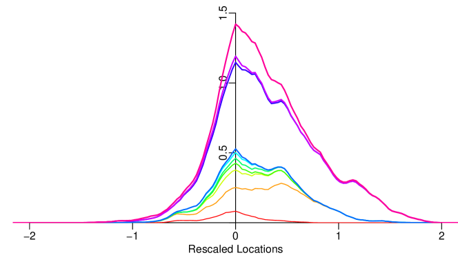
Figure 1. A simulation of $g_{s}^{N}$, for $N=1000$ and $s=0.1,0.2,\ldots,1$. The offspring and step distributions are $\nu=\text{Poi}(1)$ and $F=(\delta_{-1}+\delta_{0}+\delta_{1})/3$.

For each $N\geq 1$, the process $\{g_{s}^{N}\}_{s\geq 0}$ is nondecreasing in $s$ (relative to the natural partial ordering on $\mathcal{C}_{0}(\mathbb{R})$) and has stationary, independent increments. Therefore, the limiting process $\{g_{s}\}_{s\geq 0}$ must also be nondecreasing, with stationary, independent increments. We prove the following properties of the limiting process.

Theorem 1.4.

The limiting function-valued process $\{g_{s}\}_{s\geq 0}$ has the following properties.

1. It obeys the scaling relation $g_{s}(x)\overset{\mathcal{D}}{=\joinrel=}s^{3/2}g_{1}(x/\sqrt{s})$.

2. The real-valued process $\{I_{s}\}_{s\geq 0}$, where $I_{s}:=g_{s}(0)$ is the occupation density at zero, is a stable subordinator with exponent $\alpha=2/3$.

3. The real-valued process $\{\theta_{s}\}_{s\geq 0}$, where $\theta_{s}:=\int_{-\infty}^{\infty}g_{s}(x)dx$ is the total rescaled occupation density, is a stable subordinator with exponent $\alpha=1/2$.

4. $\{g_{s}\}_{s\geq 0}$ is a pure-jump subordinator in the Banach lattice $\mathcal{C}_{0}(\mathbb{R})$ (see Definition 3.1).

As we will show, the limiting process $g_{s}$ in Theorem 1.1 has jump discontinuities, that is, there are times $t>0$ such that the function $g_{t}-g_{t-}$ is non-zero (and hence positive) over some interval. The jumps that occur before time $t=1$ can be ordered by total area $\int(g_{t}-g_{t-})(x)\,dx$, i.e., the jump size in the stable-1/2 process $\{\theta_{s}\}_{s\geq 0}$. Denote these jumps (viewed as elements of $\mathcal{C}_{0}(\mathbb{R})$) by

$$J_{1}(x),J_{2}(x),\dots\quad\text{where}\quad\int J_{1}>\int J_{2}>\int J_{3}>\dots.$$

(In Section 3, we will see that no two jump sizes can be the same.) For each $N$, the Galton-Watson trees $\mathcal{T}_{i}$ with $i\leq N$ can also be ordered by their size (i.e., the number of vertices). The corresponding jumps in the (rescaled) occupation density $g^{N}_{s}$ will be denoted by

$$J^{N}_{1}(x),J^{N}_{2}(x),J^{N}_{3}(x),\dots.$$

(Thus, if the $j$th largest tree among the first $N$ trees is $\mathcal{T}_{\lfloor s_{j}N\rfloor}$, then $J^{N}_{j}=g^{N}_{s_{j}}-g^{N}_{\frac{\lfloor s_{j}N\rfloor-1}{N}}$.)

Corollary 1.5.

For each $m\geq 1$,

$$(J^{N}_{1},J^{N}_{2},\dots,J^{N}_{m})\Longrightarrow(J_{1},J_{2},\dots,J_{m}),$$ (1.4)

where the weak convergence is relative to the $m$-fold product topology on $\mathcal{C}_{0}(\mathbb{R})$.

Proof.

This is an immediate consequence of Theorem 1.1, because weak convergence in the Skorohod topology on $\mathbb{D}$ implies weak convergence of the ordered jump discontinuities. ∎

Theorem 1.1 can be regarded as an unconditional version of the local convergence in [5, Theorem 3.1] and [6, Theorem 1.1]. The connection between Theorem 1.1 and the results of Bousquet-Mélou/Janson and Aldous leads to a reasonably complete description of the Lévy-Khintchine representation of the pure-jump process $\{g_{s}\}_{s\geq 0}$.

Theorem 1.6.

The point process of jumps of $\{g_{s}\}_{s\geq 0}$ is a Poisson point process $\{\mathcal{N}(B)\}_{B\in\mathcal{B}}$ on the space $(\mathbb{R}_{+}\times\mathbb{R}_{+}\times\mathcal{C}_{0}(\mathbb{R}),\mathcal{B}:=\mathcal{B}_{\mathbb{R}_{+}\times\mathbb{R}_{+}\times\mathcal{C}_{0}(\mathbb{R})})$ with intensity (Lévy-Khintchine) measure

$$\chi(dt,dl,dh):=dt\cdot\frac{dl}{\sqrt{2\pi l^{3}}}\cdot f_{\textup{ISE}}(dh).$$ (1.5)

Consequently, the process $g_{s}$ can be written as

$$g_{s}(\cdot)\overset{\mathcal{D}}{=\joinrel=}\frac{1}{\sigma_{\nu}\sigma_{F}}\iiint\mathbf{1}_{[0,s]}(t)l^{3/4}h\left(l^{-1/4}\,\frac{\sigma_{\nu}}{\sigma_{F}}\cdot\,\right)\mathcal{N}(dt,dl,dh).$$ (1.6)

The remainder of the paper is organized as follows. Section 2 is devoted to the proof of Theorem 1.1, where we make use of Aldous’ stopping time criterion [1] to show the tightness of the sequence of processes $\{g^{N}_{s}\}_{s\geq 0}$. In Section 3, we prove the properties of the limiting process $g_{s}$ enumerated in Theorem 1.4 and the Lévy-Khintchine representation (1.6).

2. Proof of Theorem 1.1

2.1. Preliminaries on the Skorohod space $\mathbb{D}$

Let $(\mathcal{S},d)$ be a separable and complete metric space, and let $\mathbb{D}(\mathcal{S}){\mathrel{\hbox to0.0pt{\raisebox{1.29167pt}{$\cdot$}\hss}\raisebox{-1.29167pt}{$\cdot$}}=\,}\mathbb{D}([0,+\infty),(\mathcal{S},d))$ be the spaces of all $\mathcal{S}$-valued càdlàg functions $f$ with domain $[0,+\infty)$, i.e., $f\in\mathbb{D}(\mathcal{S})$ is right-continuous and has left limits. The space $\mathbb{D}(\mathcal{S})$ is metrizable, and under the usual Skorohod metric, the space $\mathbb{D}(\mathcal{S})$ is complete and separable. We refer to [4, Section 13] for details on the Skorohod topology. Here, we quote the following theorem, which gives a sufficient condition for the weak convergence in $\mathbb{D}(\mathcal{S})$.

Theorem 2.1.

Let $\{X_{t}^{N}\}_{t\geq 0}$ and $\{X_{t}\}_{t\geq 0}\in\mathbb{D}(\mathcal{S})$ be $\mathcal{S}$-valued processes. Let $\Delta$ be some dense subset of $[0,+\infty)$. If the sequence $\{X^{N}\}_{t\geq 0}$ is tight (relative to the Skorohod metric) and if $(X^{N}_{t_{1}},X^{N}_{{t_{2}}},\ldots,X_{t_{m}}^{N})\Longrightarrow(X_{t_{1}},X_{{t_{2}}},\ldots,X_{t_{m}})$ as $N\to\infty$ for all $t_{1},\ldots,t_{m}\in\Delta$, then $\{X^{N}_{t}\}_{t\geq 0}\Longrightarrow\{X_{t}\}_{t\geq 0}$ as $N\to\infty$.

For the particular case where $(\mathcal{S},d)$ is the real line with the Euclidean metric, Aldous [1, Theorem 1] gave a useful sufficient condition for the tightness of a sequence $\{X^{N}_{t}\}_{t\in[0,1]}$ in the space $\mathbb{D}([0,1],(\mathbb{R},\,\lvert\cdot\rvert))$. He also pointed out [2, Theorem 4.4] that, with a slight modification, the criterion can be generalized to $\mathcal{S}$-valued stochastic processes over the half line $[0,+\infty)$ as long as $(\mathcal{S},d)$ is a complete and separable metric space. We state Aldous’ criterion in this form below.

Theorem 2.2.

Let $(\mathcal{S},d)$ be a complete and separable metric space and let $\{X^{N}_{s}\}_{s\geq 0}\in\mathbb{D}([0,+\infty),(\mathcal{S},d))$ be a sequence of $\mathcal{S}$-valued stochastic processes. A sufficient condition for tightness of the sequence $\left\{X^{N}_{s}\right\}_{s\geq 0}$ is that the following two conditions hold:

Condition $1^{\circ}$. For each $s$, the sequence $\left\{X_{s}^{N}\right\}_{N\in\mathbb{N}}$ is tight in $(\mathcal{S},d)$, and
Condition $2^{\circ}$. For any $L>0$, any sequence of constant $\delta_{N}\downarrow 0$, and any sequence of stopping times $\tau_{N}$ for $\{X_{s}^{N}\}_{s\geq 0}$ that are all upper bounded by $L$,

$$d(X_{\tau_{N}+\delta_{N}}^{N},X_{\tau_{N}}^{N})\stackrel{{\scriptstyle P}}{{\longrightarrow}}0.$$ (2.1)

Remark 2.3.

In the case when $(\mathcal{S},d)=(\mathcal{C}_{0}(\mathbb{R}),\lVert\cdot\lVert_{\infty})$, (2.1) is equivalent to

$$\lVert X_{\tau_{N}+\delta_{N}}^{N}-X_{\tau_{N}}^{N}\rVert_{\infty}\stackrel{{\scriptstyle P}}{{\longrightarrow}}0.$$ (2.2)

2.2. Proof of Tightness

In this section, we prove that the sequence $\{g^{N}_{s}\}_{N\in\mathbb{N}}$ is tight in $\mathbb{D}(\mathcal{C}_{0}(\mathbb{R}))$ by verifying Condition 1^∘ and Condition $2^{\circ}$.

To verify Condition $1^{\circ}$, we will show that for any $s\geq 0$ fixed and any $\epsilon>0$, we can find a compact subset $\mathsf{K}\subset\mathcal{C}_{0}(\mathbb{R})$ such that $\mathbb{P}(g_{s}^{N}\in\mathsf{K})>1-\epsilon$ for all $N$ large. Let $\zeta_{sN}$ be the extinction time of the branching random walk gotten by amalgamating the branching random walks $(Z_{1,n})_{n\geq 0},(Z_{2,n})_{n\geq 0},\cdots,(Z_{\lfloor sN\rfloor,n})_{n\geq 0}$, that is, $\zeta_{sN}$ is the maximum of the extinction times of the branching random walks initiated by the first $\lfloor sN\rfloor$ ancestral particles. By a fundamental theorem of Kolmogorov,

$$P\left\{\zeta_{1}>n\right\}\sim\frac{2}{n\sigma_{\nu}^{2}}\quad\textrm{as}\;n\rightarrow\infty;$$

consequently, for every $\epsilon>0$, there exists $H=H_{s,\epsilon}>0$ such that

$$\mathbb{P}(\zeta_{sN}>NH)<\epsilon/2.$$ (2.3)

Therefore, it suffices to prove that there is a compact set $\mathsf{K}\subset\mathcal{C}_{0}(\mathbb{R})$ such that for all $N$ large,

$$\mathbb{P}\left(\{g_{s}^{N}\in\mathsf{K}\}\cap G_{sN}\right)\geq 1-\frac{\epsilon}{2},\quad\textrm{where}\quad G_{sN}:=\left\{\zeta_{sN}\leq NH\right\}.$$ (2.4)

To establish inequality (2.4) we will use Kolmogorov-Čentsov criterion (see, e.g., [8, Chapter 2, Problem 4.11]). It suffices to prove that

$$\sup_{N}\mathbb{E}[g_{s}^{N}(0)\mathbf{1}_{G_{sN}}]<\infty,$$ (2.5a)

and that for some $m\geq 3$, there exists $C=C(s,m,H)>0$ such that for all $x,y\in\mathbb{R}$ and for all $N$ sufficiently large,

$$\mathbb{E}\left[g_{s}^{N}(x)-g_{s}^{N}(y)\right]^{2m}\mathbf{1}_{G_{sN}}\leq C|x-y|^{\frac{2m}{5}}.$$ (2.5b)

Note that the requirement $m\geq 3$ in (2.5b) ensures that the exponent $2m/5$ is larger than $1$, as is needed for the Kolmogorov-Čentsov criterion. We will rely on the following estimates of [10] to compute these bounds.

Proposition 2.4.

[10, Proposition 5] Let $Z_{n}(x)$ be the number of particles at location $x\in\mathbb{Z}$ and time $n\in\mathbb{Z}_{+}$ in a branching random walk, started from a single particle at $0\in\mathbb{Z}$, with offspring distribution $\nu$ and step distribution $F$. For each $m\in\mathbb{N}$, there is constant $C_{m}$ such that for all $x,y\in\mathbb{Z}$ and all $n\geq 1$,

$$\mathbb{E}Z_{n}(x)^{m} \leq C_{m}n^{m/2-1}$$ (2.6)

$$|\mathbb{E}(Z_{n}(x)-Z_{n}(y))^{m}| \leq C_{m}n^{2m/5-1}|x-y|^{m/5}$$ (2.7)

Corollary 2.5.

Let $Z_{n}(x)$ be as in Proposition 2.4. Then, for any $H>0$ and $m\geq 1$, there exists $C=C_{m,H}$ such that for all $N\geq 1$ and $x,y\in\mathbb{Z}/\sqrt{N}$,

$$\sum_{n_{1},\ldots,n_{m}=1}^{\lfloor NH\rfloor}\left|\mathbb{E}\prod_{l=1}^{m}\left(Z_{n_{l}}(\sqrt{N}x)-Z_{n_{l}}(\sqrt{N}y)\right)\right|\leq C|x-y|^{\frac{m}{5}}N^{\frac{3m}{2}-1}.$$ (2.8)

Proof.

Suppose first $m$ is even. Then by a trivial extension of Hölder’s inequality (see, e.g.,[13, pp. 4]) and Proposition 2.4,

$$\ \ \ \ \ \sum_{n_{1},\ldots,n_{m}=1}^{\lfloor NH\rfloor}\left|\mathbb{E}\prod_{l=1}^{m}\left(Z_{n_{l}}(\sqrt{N}x)-Z_{n_{l}}(\sqrt{N}y)\right)\right|$$

$$\leq\sum_{n_{1},\ldots,n_{m}=1}^{\lfloor NH\rfloor}\prod_{l=1}^{m}\left|\mathbb{E}\left(Z_{n_{l}}(\sqrt{N}x)-Z_{n_{l}}(\sqrt{N}y)\right)^{m}\right|^{\frac{1}{m}}$$

$$=\left\{\sum_{n_{1}=1}^{\lfloor NH\rfloor}\left|\mathbb{E}\left(Z_{n_{1}}(\sqrt{N}x)-Z_{n_{1}}(\sqrt{N}y)\right)^{m}\right|^{\frac{1}{m}}\right\}^{m}$$

$$\leq\left\{\sum_{n_{1}=1}^{\lfloor NH\rfloor}\left[C_{m}n_{1}^{\frac{2m}{5}-1}|x-y|^{\frac{m}{5}}N^{\frac{m}{10}}\right]^{\frac{1}{m}}\right\}^{m}$$

$$\leq C_{m,H}|x-y|^{\frac{m}{5}}N^{\frac{3m}{2}-1}.$$

The case when $m$ is odd is similar. ∎

Proof of Condition 1^∘.

The bound in (2.5a) is easy to check using (2.6) with $m=1$ and $x=0$ and the linearity of expectation. In particular,

$$\mathbb{E}[g_{s}^{N}(0)\mathbf{1}_{G_{sN}}] \leq\frac{sN}{N^{3/2}}\left(1+\sum_{n=1}^{NH}C_{1}n^{1/2-1}\right)=\frac{s}{\sqrt{N}}\left(1+O(\sqrt{N})\right)<\infty.$$

For (2.5b), first of all, by triangle inequality and the assumption that $\bar{X}^{N}(x)$ is defined by linear interpolation, we need only consider $x,y\in\mathbb{Z}/\sqrt{N}$ in (2.5b).

Let $Z_{i,n}(x)$ be the number of particles at site $x\in\mathbb{Z}$ in generation $n$ of the $i$-th ancestral particle. The left side of (2.5b) is clearly bounded by

$$N^{-3m}\cdot\mathbb{E}\left\{\sum_{i=1}^{\lfloor sN\rfloor}\sum_{n=0}^{\lfloor NH\rfloor}\left[Z_{i,n}(\sqrt{N}x)-Z_{i,n}(\sqrt{N}y)\right]\right\}^{2m}.$$

We expand the product under the expectation sign and write it as a sum of expectations:

$$N^{-3m}\cdot\sum_{i_{1},\ldots,i_{2m}=1}^{\lfloor sN\rfloor}\sum_{n_{1},\ldots,n_{2m}=0}^{\lfloor NH\rfloor}\mathbb{E}\prod_{j=1}^{2m}\left[Z_{i_{j},n_{j}}^{\lfloor sN\rfloor}(\sqrt{N}x)-Z_{i_{j},n_{j}}^{\lfloor sN\rfloor}(\sqrt{N}y)\right].$$ (2.9)

When the product inside the expectations is expanded, each term is a product of $2m$ differences of occupation counts in one of the branching random walks $Z_{i_{j}}$ in some generation $n_{j}$. Observe that repetitions of the indices $i_{j}$ and $n_{j}$ are allowed.

Note that Proposition 2.4 applies only for generation $n\geq 1$, whereas $n_{1},\ldots,n_{2m}$ in (2.9) run from generation $0$. However, since originally all particles are placed at the origin, we lose nothing by summing from $1$ to $\lfloor NH\rfloor$ as long as $xy\neq 0$. The case when $xy=0$ will be treated separately at the end.

Suppose $x\neq 0$, $y\neq 0$. If $i_{j_{1}}\neq i_{j_{2}}$ are indices of two distinct ancestral individuals, then the differences $\left[Z_{i_{j_{1}},n_{j_{1}}}(\sqrt{N}x)-Z_{i_{j_{1}},n_{j_{1}}}(\sqrt{N}y)\right]$ and $\left[Z_{i_{j_{2}},n_{j_{2}}}(\sqrt{N}x)-Z_{i_{j_{2}},n_{j_{2}}}(\sqrt{N}y)\right]$ are independent. Let $r$ be the number of distinct $i_{j}$’s inside the expectation in (2.9); then (2.9) can be written as

$$N^{-3m}\sum_{r=1}^{2m}\sum_{\begin{subarray}{c}1\leq i_{1}<\cdots<i_{r}\leq\lfloor sN\rfloor\\ \sum_{j}m_{j}=2m\end{subarray}}\prod_{j=1}^{r}\left[\sum_{n^{j}_{1}\ldots n^{j}_{m_{j}}=1}^{\lfloor NH\rfloor}\mathbb{E}\prod_{l=1}^{m_{j}}\left(Z_{i_{j},n^{j}_{l}}(\sqrt{N}x)-Z_{i_{j},n^{j}_{l}}(\sqrt{N}y)\right)\right].$$ (2.10)

For a particular term with $r$ distinct ancestors $i_{1},\ldots,i_{r}$ in which $i_{j}$ occurs $m_{j}$ times ($j=1,2,\ldots,r$), the expectation can be factored as a product of $r$ expectations, where each expectation is an expectation of the differences involving the offspring of only one ancestor at time 0. Thus, we always have $\sum_{j=1}^{r}m_{j}=2m$. For each bracketed factor in (2.10), for each ancestor $i_{j}$, the summation is over all possible choices of the generations $n_{1}^{j},\ldots,n_{m_{j}}^{j}$; this can be bounded using Corollary 2.5 above. It follows that

$$\ \ N^{-3m}\sum_{r=1}^{2m}\sum_{\begin{subarray}{c}1\leq i_{1}<\cdots<i_{r}\leq\lfloor sN\rfloor\\ \sum_{j}m_{j}=2m\end{subarray}}\prod_{j=1}^{r}C(m_{j},H)|x-y|^{\frac{m_{j}}{5}}N^{\frac{3m_{j}}{2}-1}$$

$$\leq\ C_{1}(m,s,H)\,N^{-3m}\sum_{r=1}^{2m}N^{r}\cdot N^{\frac{3}{2}\cdot 2m-r}|x-y|^{\frac{2m}{5}}$$

$$\leq\ C(m,s,H)|x-y|^{\frac{2m}{5}},$$

and (2.5b) is proved.

Finally, we must deal with the case when $xy=0$. If $x=y=0$, then both sides of (2.5b) are zero. If $x=0$ and $y\neq 0$, then, because all initial $\lfloor sN\rfloor$ particles are placed at zero, we can write the left side of (2.5b) as

$$\mathbb{E}\left\{\left(\sum_{i=1}^{\lfloor sN\rfloor}\sum_{n=1}^{NH}\frac{\left[Z_{i,n}(0)-Z_{i,n}(\sqrt{N}y)\right]}{N^{3/2}}\right)+\frac{\lfloor sN\rfloor}{N^{3/2}}\right\}^{2m}.$$

It is not difficult to see that for large $N$, the first term dominates, because this term can be handled exactly as in the case $xy\not=0$. This proves that Condition 1^∘ holds. ∎

Proof of Condition 2^∘.

For each $N$ the process $g^{N}_{s}$ is piecewise constant in $s$, with jumps only at times $s$ that are integer multiples of $1/N$. Consequently, in verifying Condition 2 we may restrict attention to stopping times $\tau_{N}$ such that $N\tau_{N}$ is an integer between $0$ and $NL$. It is obvious from its definition that the discrete-time process $g^{N}_{s}$, with $s=0,1/N,2/N,\cdots$, is non-decreasing and has stationary, independent increments; therefore, for any stopping time $\tau^{N}$ and any constant $\delta>0$, the increment $g^{N}_{\tau_{N}+\delta}-g^{N}_{\tau_{N}}$ has the same distribution as $g^{N}_{\delta}$. Therefore, to prove Condition 2^∘ it is enough to show that for any $\epsilon>0$ there exists $\delta>0$ such that for all $N$ sufficiently large,

$$\mathbb{P}\left(\sup_{x\in\mathbb{R}}g_{\delta}^{N}(x)\geq\epsilon\right)\leq\epsilon,$$

equivalently,

$$\mathbb{P}\left(\sup_{x\in\mathbb{R}}g_{1}^{\lfloor\delta N\rfloor}(x)\geq\epsilon\delta^{-3/2}\right)\leq\epsilon.$$ (2.11)

But we have already proved, in Condition 1^∘, that the sequence of $\mathcal{C}_{0}(\mathbb{R})-$valued processes $g^{N}_{1}$ is tight, so there exists $K=K_{\epsilon}<\infty$ so large that for all $m\in\mathbb{N}$,

$$\mathbb{P}\left(\sup_{x\in\mathbb{R}}g_{1}^{m}(x)\geq K\right)\leq\epsilon.$$

By choosing $\delta>0$ so small that $\epsilon/\delta^{3/2}>K$, we obtain (2.11) for $N$ sufficiently large. ∎

2.3. Uniqueness of the Limit Process

Since $\{g_{s}^{N}\}_{s\geq 0}$ has stationary and independent increments, any weak limit will also have these properties. Therefore, to prove the uniqueness of the limit process it suffices to show that for any fixed time $s>0$ there is only one possible limit for the sequence $\{g^{N}_{s}\}_{N\in\mathbb{N}}$.

For any $N\in\mathbb{N}$, the random function $g^{N}_{s}(\cdot)$ is defined by rescaling the occupation measure $X^{\lfloor sN\rfloor}$ of the branching random walk initiated by the first $\lfloor sN\rfloor$ ancestral individuals (cf. equation (1.2)). The occupation measure $X^{\lfloor sN\rfloor}$ is defined by (1.1), which can be rewritten as

$$X^{m}(j)=\sum_{i=1}^{m}\sum_{n=0}^{\infty}Z_{i,n}(j),$$

where $Z_{i,n}(j)$ is the occupation counts at location $j$ of individuals in the $n$-th generation of the $i$-th labeled tree. As discussed in Remark 1.3, to avoid invoking an indefinite integral operator in the weak limit, we consider the truncated occupation counts and the associated occupation density up to the $\lfloor NH\rfloor$-th generation for some $H>0$ fixed. Define

$$X^{m,H}(j) =\sum_{i=1}^{m}\sum_{n=0}^{\lfloor NH\rfloor}Z_{i,n}(j)\quad\textrm{and}$$

$$g^{N}_{s,H}(x) =N^{-3/2}\bar{X}^{\lfloor sN\rfloor,H}(\sqrt{N}x)$$

where, as earlier, the bar denotes the function obtained by linear interpolation. The same calculations as in the proof of Condition 1^∘ show that for any fixed $H>0$ and $s>0$ the sequence $g^{N}_{s,H}$ is tight.

Watanabe’s convergence theorem states that for any $s>0$, the rescaled measure-valued process converges weakly to the super-Brownian motion, i.e.,

$$\left\{Y_{t}^{s,N}\right\}_{0\leq t\leq H}:=\left\{\frac{1}{N}\sum_{j\in\mathbb{Z}}\sum_{i=1}^{\lfloor Ns\rfloor}Z_{i,\lfloor tN\rfloor}(j)\delta_{j/\sqrt{N}}\right\}\Longrightarrow\left\{Y_{t}^{s}\right\}_{0\leq t\leq H},$$

Viewing the measure-valued process $Y_{t}^{s,N}$ as nonnegative continuous functions over $\mathbb{R}$, we define $\bar{Y}_{t}^{s,N}\in\mathcal{C}_{0}(\mathbb{R})$ by setting

$$\bar{Y}_{t}^{s,N}(x):=\frac{1}{N}\sum_{i=1}^{\lfloor Ns\rfloor}Z_{i,\lfloor tN\rfloor}(\sqrt{N}x),\quad\text{if }x\in\mathbb{Z}/\sqrt{N}.$$

and then doing a linear interpolation. The above convergence implies that the weak convergence of the rescaled total occupation measure of the first $\lfloor NH\rfloor$ generations:

$$\frac{1}{N}\sum_{t=0}^{\lfloor NH\rfloor}Y^{s,N}_{\frac{t}{N}}(x)\Longrightarrow\int_{0}^{H}Y_{t}^{s}(x)dt.$$

Notice that the left side is indeed $\frac{X^{\lfloor sN\rfloor,H}(\sqrt{N}x)}{N^{2}}$, which has densities $g^{N}_{s,H}$. Consequently, any possible weak subsequential limit of $\{g^{N}_{s,H}\}_{N\geq 1}$ in the function space $\mathcal{C}_{0}(\mathbb{R})$ must be a density for the occupation measure of the super-Brownian motion, that is, as $N\to\infty$

$$g^{N}_{s,H}\Longrightarrow g_{s,H}\quad\textrm{where}\quad g_{s,H}(x){\mathrel{\hbox to0.0pt{\raisebox{1.29167pt}{$\cdot$}\hss}\raisebox{-1.29167pt}{$\cdot$}}=\,}\int_{0}^{H}Y^{s}(t,x)dt.$$

But by inequality (2.3), for any $\epsilon>0$ there exists $H=H_{\epsilon}<\infty$ so large that for any $N$,

$$\mathbb{P}\left\{g^{N}_{s}\not=g^{N}_{s,H}\right\}\leq\epsilon.$$

Consequently, the sequence $\{g^{N}_{s}\}_{N\in\mathbb{N}}$ must converge weakly to $\int_{0}^{\infty}Y^{s}(t,x)dt$.

3. Properties of the Limiting Process

In this section, we prove properties of the limiting process $\{g_{s}\}_{s\geq 0}$ (Theorem 1.4) and characterize it using a Poisson point process (Theorem 1.6). In order to make sense of the notion of a “subordinator” on the function space $\mathcal{C}_{0}(\mathbb{R})$, we first briefly review the definition of a Banach lattice.

Definition 3.1.

A Banach lattice is a triple $(E,\lVert\cdot\rVert,\leq)$ such that

1. $(E,\lVert\cdot\rVert)$ is a Banach space with norm $\lVert\cdot\rVert$;

2. $(E,\leq)$ is an ordered vector space with the partial ordering $\leq$;

3. under $\leq$, any pair $x,y\in E$ has a least upper bound denoted by $x\vee y$ and a greatest lower bound denoted by $x\wedge y$ (this is the “lattice” property); and

4. Set $|x|{\mathrel{\hbox to0.0pt{\raisebox{1.29167pt}{$\cdot$}\hss}\raisebox{-1.29167pt}{$\cdot$}}=\,}x\vee(-x)$. Then $|x|\leq|y|$ implies $\lVert x\rVert\leq\lVert y\rVert$, $\forall x,y\in E$ (i.e., $\lVert\cdot\rVert$ is “a lattice norm”).

Example 1.

The Banach space $(\mathcal{C}_{0}(\mathbb{R}),\lVert\cdot\rVert_{\infty})$ has a natural partial ordering, defined by

$$f\leq g\textup{ if and only if }g(x)-f(x)\geq 0\quad\text{for all}\quad x\in\mathbb{R}.$$

The triple $(\mathcal{C}_{0}(\mathbb{R}),\lVert\cdot\rVert_{\infty},\leq)$ clearly satisfies (a) and (b) in Definition 3.1. The least upper bound and the greatest lower bound are defined pointwise:

$$(f\vee g)(x)=f(x)\vee g(x),\qquad(f\wedge g)(x)=f(x)\wedge g(x).$$

Condition (d) can be verified easily.

Definition 3.2.

Let $(E,\lVert\cdot\rVert,\leq)$ be a Banach lattice. An $E$-valued stochastic process $\{X_{t}\}_{t\geq 0}$ is a subordinator if $\{X_{t}\}_{t\geq 0}$ is a Lévy process (that is, $\{X_{t}\}_{t\geq 0}$ has stationary, independent increments) and with probability one, for all $t\geq s\geq 0$,

$$X_{t}-X_{s}\geq 0.$$

A subordinator $\{X_{t}\}_{t\geq 0}$ is a pure jump process if for every $t$,

$$X_{t}=\sum_{s\leq t}(X_{s}-X_{s-}).$$

Proof of Theorem 1.4.

For (i), we have for each $N\geq 1$,

$$g_{s}^{N}(x)=\frac{\bar{X}^{\lfloor sN\rfloor}(\sqrt{N}x)}{N^{3/2}}=\frac{\lfloor sN\rfloor^{3/2}}{N^{3/2}}\cdot\frac{\bar{X}^{1\cdot\lfloor sN\rfloor}\left(\sqrt{N}x\right)}{\lfloor sN\rfloor^{3/2}}=\frac{\lfloor sN\rfloor^{3/2}}{N^{3/2}}g_{1}^{\lfloor sN\rfloor}\left(\sqrt{\frac{N}{\lfloor sN\rfloor}}\,x\right).$$

Taking $N\to\infty$ gives (i). The claim that $\{I_{s}\}_{s\geq 0}$ is a stable-2/3 subordinator follows from monotonicity of $g_{s}$ and the scaling relation above at $x=0$, which yields

$$I_{s}=s^{3/2}I_{1}.$$

For (iii), recall that a version of the stable–$\frac{1}{2}$ subordinator on $\mathbb{R}$ is the inverse local-time process of a standard Brownian motion $\{B_{t}\}_{t\geq 0}$

$$\tilde{\tau}_{s}=\inf\{t\geq 0\,:\,L^{0}_{t}>s\},$$

where $L^{0}_{t}$ is the Brownian local time at location $0$ up to time $t$. The jumps of the process $\{\tilde{\tau}_{s}\}_{s\geq 0}$ are the lengths of the excursions of the Brownian path.

Now consider a sequence of independent critical Galton-Watson trees $\mathcal{T}_{i}$ with offspring distribution $\nu$, initiated by particles $i=1,2,3,\dots$. Let $|\mathcal{T}_{i}|$ be the size (number of vertices) of the $i$-th tree, and set $A_{N}{\mathrel{\hbox to0.0pt{\raisebox{1.29167pt}{$\cdot$}\hss}\raisebox{-1.29167pt}{$\cdot$}}=\,}\sum_{i=1}^{N}|\mathcal{T}_{i}|$, the total number of vertices in the first $k$ trees. Then by a theorem of Le Gall [11], as $N\to\infty$,

$$\{A_{\lfloor sN\rfloor}/N^{2}\}_{s\geq 0}\Longrightarrow\{\tilde{\tau}_{s/\sigma_{\nu}}\}_{s\geq 0}\overset{\mathcal{D}}{=\joinrel=}\{\sigma_{\nu}^{-2}\tilde{\tau}_{s}\}_{s\geq 0},$$

where the last equality follows from the scaling rule of a stable–$\frac{1}{2}$ process.

Next, suppose that branching random walks are built on the Galton-Watson trees $\mathcal{T}_{i}$ by labelling the vertices, as described earlier. Then clearly

$$A_{\lfloor sN\rfloor}=\sum_{j\in\mathbb{Z}/\sqrt{N}}X^{\lfloor sN\rfloor}(\sqrt{N}j).$$

By Theorem 1.1, $\{g_{s}^{N}\}_{s\geq 0}\Rightarrow\{g_{s}\}_{s\geq 0}$ in $\mathbb{D}([0,+\infty),\mathcal{C}_{0}(\mathbb{R}))$. Considering the space-truncated occupation density $g_{s}^{N}(x)\mathbf{1}_{[-B,B]}(x)$ (i.e., truncated in space) for sufficiently large $B>0$ and following the same strategy as when proving the uniqueness of the limiting process $\{g_{s}\}_{s\geq 0}$, one would obtain

$$\left\{\frac{1}{\sqrt{N}}\sum_{x\in\mathbb{Z}/\sqrt{N}}g_{s}^{N}(x)\right\}_{s\geq 0}\Longrightarrow\left\{\int_{\mathbb{R}}g_{s}(x)dx\right\}_{s\geq 0}:=\{\theta_{s}\}_{s\geq 0},$$

where the left side is indeed

$$\frac{1}{\sqrt{N}}\sum_{x\in\mathbb{Z}/\sqrt{N}}g_{s}^{N}(x)=\frac{\sum_{x\in\mathbb{Z}/\sqrt{N}}X^{\lfloor sN\rfloor}(\sqrt{N}x)}{N^{2}}=\frac{A_{\lfloor sN\rfloor}}{N^{2}}.$$

Consequently, the processes $\{\theta_{s}\}_{s\geq 0}$ and $\{\sigma_{\nu}^{-2}\tilde{\tau}_{s}\}_{s\geq 0}$ have the same law, and so $\{\theta_{s}\}_{s\geq 0}$ is a stable-1/2 subordinator.

For (iv), we have already observed that $g_{s}$ has stationary, independent increments and increasing sample paths relative to the natural partial order $\leq$ on $\mathcal{C}_{0}(\mathbb{R})$. To show that $\{g_{s}\}_{s\geq 0}$ has pure jumps, we make use of the fact that the total area process $\{\theta_{s}\}_{s\geq 0}$ is a stable–$\frac{1}{2}$ subordinator and thus has pure jumps. Let $\mathcal{J}$ be the set of jump times of the process $\{\theta_{s}\}_{s\geq 0}$, that is, the set of all $t\geq 0$ for which $\theta(t)-\theta(t-)>0$. Define

$$\tilde{g}_{s}=\sum_{t\in\mathcal{J}\cap[0,s]}(g_{t}-g_{t-}),$$

a process that collects the changes in $\{g_{s}\}_{s\geq 0}$ at those times when the limiting total area process $\{\theta_{s}\}_{s\geq 0}$ makes jumps. Clearly, the process $\tilde{g}_{s}$ is an increasing process in $\mathcal{C}_{0}(\mathbb{R})$, and since $\tilde{g}_{s}$ only gathers the jumps of $g_{s}$, we have

$$\tilde{g}_{s}\leq g_{s}\quad\text{for every}\;\;s\geq 0.$$

But since the area process $\theta_{s}$ is pure jump, $g_{s}$ and $\tilde{g}_{s}$ bound the same total area for every $s$, that is,

$$\int_{\mathbb{R}}g_{s}(x)\,dx=\theta_{s}=\int_{\mathbb{R}}\tilde{g}_{s}(x)\,dx.$$

By continuity of both $g_{s}$ and $\tilde{g}_{s}$, we have $g_{s}=\tilde{g}_{s}$ for every $s$, and thus the process $g_{s}$ is a pure jump process in $\mathcal{C}_{0}(\mathbb{R})$.

∎

Proof of Theorem 1.6.

We have already proved in Theorem 1.4 that the process $g_{s}$ consists of pure jumps. It remains to show that the point process of jumps is a Poisson point process with intensity given by (1.5) and then the representation (1.6) would follow automatically.

Consider the point process of jumps of $g_{s}$ for $s\leq 1$ (the case $s\leq s_{*}$, for arbitrary $s_{*}>0$, can be handled in analogous fashion). Let $J_{1},J_{2},\dots$ be the jumps ordered by size from largest to smallest, as in Corollary 1.5. Since by Theorem 1.4, the limiting process $\{g_{s}\}_{s\geq 0}$ is a pure jump subordinator, we have

$$g_{1}=\sum_{i=1}^{\infty}J_{i}.$$ (3.1)

Theorem 1.4 also implies that the jump sizes $|J_{i}|=\int J_{i}(x)\,dx$ are distributed (jointly) as the ordered excursion lengths of a standard Brownian motion run up to the first time $t$ that $L^{0}_{t}=1$, rescaled by $\sigma_{\nu}^{-2}$. By Corollary 1.5, for any $m\geq 1$, as $k\rightarrow\infty$,

$$(J^{N}_{1},J^{N}_{2},\dots,J^{N}_{m})\Longrightarrow(J_{1},J_{2},\dots,J_{m}),$$ (3.2)

where $J^{N}_{1},J^{N}_{2},\dots$ are the ordered jumps in the (rescaled) occupation density processes $g^{N}_{s}$ for $s\leq 1$ for the branching random walk obtained by amalgamating the first $N$ trees. Consequently, the joint distribution of the random variables

$$|J^{N}_{i}|=|\mathcal{T}^{N}_{(i)}|/N^{2}$$

(where $\mathcal{T}^{N}_{(i)}$ is the $i$-th largest tree among the first $N$ trees) converges to the joint distribution of the sizes $|J_{i}|$. In particular, the largest, second largest, etc., trees among the first $N$ trees have sizes of order $N^{2}$ — and so as $N\rightarrow\infty$, these will be large.

To identify the limiting distribution of the rescaled jumps, we now make use of Theorem 1.1 in [6], which states that the occupation density of a conditioned branching random walk scaled by the size of the tree converges to that of the ISE density $f_{\textup{ISE}}$, as the size of the tree becomes large. This implies, for each $i=1,2,\dots$, as $N\rightarrow\infty$,

$$\frac{J^{N}_{i}(|J_{i}^{N}|^{1/4}\ \cdot\,)}{|J_{i}^{N}|^{3/4}}\Longrightarrow\gamma f^{(i)}_{\textup{ISE}}(\gamma\ \cdot\,),\ \ \text{where }\gamma=\sigma_{F}^{-1}\sigma_{\nu}^{1/2},$$ (3.3)

and the limiting ISE densities, $f^{(1)}_{\textup{ISE}}$, $f^{(2)}_{\textup{ISE}}$, $\ldots$ are i.i.d copies of $f_{\textup{ISE}}$. By (3.2) and (3.3), we can describe the joint distribution of $J_{1},J_{2},\dots$ as follows: (a) let $\varepsilon_{1}>\varepsilon_{2}>\varepsilon_{3}>\dots$ be the ordered excursion lengths of a standard Brownian motion run until the first time $t$ such that $L^{0}_{t}=1$; (b) let $f_{1},f_{2},f_{3},\dots$ be i.i.d. copies of the ISE density $f_{\textup{ISE}}$ which are independent of the $\varepsilon_{i}$’s; and (c) set

$$J_{i}(\cdot) {\mathrel{\hbox to0.0pt{\raisebox{1.29167pt}{$\cdot$}\hss}\raisebox{-1.29167pt}{$\cdot$}}=\,}(\sigma_{\nu}^{-2}\varepsilon_{i})^{3/4}\gamma f_{i}(\gamma(\sigma_{\nu}^{-2}\varepsilon_{i})^{-1/4}\ \cdot\,)$$

$$=\frac{1}{\sigma_{\nu}\sigma_{F}}\,\varepsilon_{i}^{3/4}f_{i}(\sigma_{\nu}\sigma_{F}^{-1}\varepsilon_{i}^{-1/4}\ \cdot\,).$$

Since the ordered excursion lengths $\varepsilon_{1}>\varepsilon_{2}>\varepsilon_{3}>\dots$ have the distribution of the ordered points in a Poisson point process on $\mathbb{R}_{+}$ with intensity measure $\frac{dy}{\sqrt{2\pi y^{3}}},$ the representation (1.6) follows from (3.1).

∎

Acknowledgment. The authors are grateful to the anonymous referee for valuable comments.

References

- [1] D. Aldous, Stopping times and tightness, Ann. Probab. 6 (1978), no. 2, 335–340. MR 0474446
- [2] D. Aldous, Weak convergence and the general theory of processes, preprint (1983).
- [3] D. Aldous, Tree-based models for random distribution of mass, J. Statist. Phys. 73 (1993), no. 3-4, 625–641. MR 1251658
- [4] P. Billingsley, Convergence of probability measures, second ed., Wiley Series in Probability and Statistics: Probability and Statistics, John Wiley & Sons, Inc., New York, 1999, A Wiley-Interscience Publication. MR 1700749
- [5] M. Bousquet-Mélou and S. Janson, The density of the ISE and local limit laws for embedded trees, Ann. Appl. Probab. 16 (2006), no. 3, 1597–1632. MR 2260075
- [6] L. Devroye and S. Janson, Distances between pairs of vertices and vertical profile in conditioned Galton-Watson trees, Random Structures & Algorithms 38 (2011), no. 4, 381–395. MR 2829308
- [7] A. M. Etheridge, An introduction to superprocesses, University Lecture Series, vol. 20, American Mathematical Society, Providence, RI, 2000. MR 1779100
- [8] I. Karatzas and S. E. Shreve, Brownian motion and stochastic calculus, second ed., Graduate Texts in Mathematics, vol. 113, Springer-Verlag, New York, 1991. MR 1121940
- [9] N. Konno and T. Shiga, Stochastic partial differential equations for some measure-valued diffusions, Probab. Theory Related Fields 79 (1988), no. 2, 201–225. MR 958288
- [10] S. P. Lalley, Spatial epidemics: critical behavior in one dimension, Probab. Theory Related Fields 144 (2009), no. 3-4, 429–469. MR 2496439
- [11] J.-F. Le Gall, Random trees and applications, Probab. Surv. 2 (2005), 245–311. MR 2203728
- [12] J.-F. Marckert, The rotation correspondence is asymptotically a dilatation, Random Structures & Algorithms 24 (2004), no. 2, 118–132. MR 2035871
- [13] O. Pons, Inequalities in analysis and probability, World Scientific Publishing Co. Pte. Ltd., Hackensack, NJ, 2013. MR 3012196
- [14] S. Watanabe, A limit theorem of branching processes and continuous state branching processes, J. Math. Kyoto Univ. 8 (1968), 141–167. MR 0237008