Anomalous energy transport in laminates with exceptional points

Abstract

Recent interest in metamaterials has led to a renewed study of wave mechanics in different branches of physics. Elastodynamics involves a special intricacy, owing to a coupling between the volumetric and shear parts of the elastic waves. Through a study of in-plane waves traversing periodic laminates, we here show that this coupling can result with unusual energy transport. We find that the corresponding frequency spectrum contains modes which simultaneously attenuate and propagate, and demonstrate that these modes coalesce to purely propagating modes at exceptional points—a property that was recently reported in parity-time symmetric systems. We show that the laminate exhibits metamaterial features near these points, such as negative refraction, and beam steering and splitting. While negative refraction in laminates has been demonstrated before by considering pure shear waves impinging an interface with multiple layers, here we realize it for coupled waves impinging a simple single-layer interface. This feature, together with the appearance of exceptional points, are absent from the model problem of anti-plane shear waves which have no volumetric part, and hence from the mathematically identical electromagnetic waves. Our work further paves the way for applications such as asymmetric mode switches, by encircling exceptional points in a tangible, purely elastic apparatus.

Keywords: metamaterial, negative refraction, wave propagation, Bloch-Floquet waves, composite, laminate, phononic crystal, exceptional points

1 Introduction

Metamaterials possess properties not found in nature, stemming from their architectured microstructure (Wegener, 2013, Kadic et al., 2019). Perhaps the most prominent thrust in metamaterials research aims at controlling waves for potential applications such as lensing, cloaking and noise reduction (Milton et al., 2006, Chen et al., 2010, Parnell and Shearer, 2013, Bigoni et al., 2013, Colquitt et al., 2014, Cummer et al., 2016). This interest led to a renewed study of wave mechanics in optics (Markos and Soukoulis, 2008, Banerjee, 2011), acoustics (Craster and Guenneau, 2012, Deymier, 2013), mechanical lattices (Phani, 2011, Raney et al., 2016, Phani and Hussein, 2017, Zelhofer and Kochmann, 2017, Ma et al., 2018) and elastodynamics (Brun et al., 2010, Shmuel and Band, 2016, Chen and Elbanna, 2017, Aghighi et al., 2019, Li and Reina, 2019).

While electromagnetic-, sound- and anti-plane shear waves are mathematically identical (Adams et al., 2008, Torrent and Sánchez-Dehesa, 2011), in-plane elastic waves are physically richer (Sigalas and Economou, 1992), since they comprise both volumetric and distortional parts, coupled through interfaces in the transmission medium. In this work, we show that in the simplest elastic composite—a laminate—this coupling gives rise to anomalous energy transport, which in other systems is achieved by significantly more complicated means. The anomalies reported here and their connection with recent studies in the field are summarized next.

Firstly, we show that the spectrum of in-plane waves in laminates exhibits exceptional points, accessible in a purely elastic setting. Exceptional points are states of a system at which two (or more) of its normal modes coalesce, together with their natural frequencies (Moiseyev and Friedland, 1980, Ding et al., 2015), and are the source of counterintuitive phenomena such as enhanced sensitivity, wave stopping and asymmetric transmission (Hodaei et al., 2017, Achilleos et al., 2017, Goldzak et al., 2018, Merkel et al., 2018). Exceptional points occur only in non-Hermitian systems (Moiseyev, 2011), a property which usually describes systems that interact with the environment. The current paradigm to access exceptional points is by balancing external gain and loss through the system, to create parity-time ($\mathcal{PT}$) symmetry (Rüter et al., 2010, Shi et al., 2016, El-Ganainy et al., 2018). This procedure brings with additional complexity to the elastic medium, as such realizations require incorporating optomechanical, acoustoelectric or piezoelectric elements into the system (Xu et al., 2015, Christensen et al., 2016, Hou and Assouar, 2018). Our findings thus suggest a simpler, purely elastic setting to access exceptional points, thereby evading these complexities.

Recently, it was demonstrated that encircling these points leads to fascinating asymmetric mode switching of microwaves in a metallic waveguide (Doppler et al., 2016). We argue that our setting constitutes a tangible platform to realize analogous encirclement for elastic wave switching, having the wavenumber, which is related to the excitation angle, as the trajectory parameter. As we show in the sequel, this is made possible owing to the intrinsic Riemann surface structure of our spectrum near these points in the complex wave vector space. In contrast with cases where this structure is artificially obtained by an analytical continuation of an arbitrary parameter (e.g., the frequency in Shanin et al., 2018), here, complex wavenumbers are an intrinsic and accessible part of the spectrum.

Secondly, we demonstrate that the exceptional points foreshadow anomalous energy transport, including negative refraction. In this regard, perhaps our most striking result is the excitation of negative refraction in laminates by an incoming wave from a homogeneous medium whose interface with the laminate is parallel to the layers (Fig.  1). To put this result into context, we recall that the first report of negative refraction was for electromagnetic waves, and required a two-dimensional composite made of complicated split ring resonators (Smith et al., 2000, Shelby et al., 2001, Pendry, 2004). Interest in this phenomenon has been disseminated to elastodynamics, accompanied with ongoing studies (Craster and Guenneau, 2012, Chen et al., 2017, Bordiga et al., 2019, Nemat-Nasser, 2019). Notably, Willis (2013) was the first to show that a simple laminate is capable of negatively refracting anti-plane shear waves. While in the conventional arrangement (interface parallel to the layers), refraction is always positive, Willis realized that negative refraction is possible when the interface is normal to the layers (Fig.  1c). Based on this interface configuration, further studies of such waves in laminated media were carried out (Willis, 2015, Nemat-Nasser, 2015, Srivastava, 2016, Morini et al., 2019). Hence, we demonstrate that in-plane waves may refract negatively in the conventional arrangement, without the need for this complex apparatus, nor for gain and loss (cf.  Hou et al., 2018).

For completeness, we also analyze the transmission problem through an interface normal to the layers. As highlighted by Srivastava and Willis (2017) and the references therein, a wave incident to such interface induces an infinite number of transmitted waves, which are required to satisfy corresponding continuity conditions across the interface. We suggest a method to calculate the resultant normal mode decomposition owing to incident in-plane waves, based on suitable orthogonality conditions (Mokhtari et al., 2019). Subsequently, we demonstrate analogous phenomena to those reported by Srivastava (2016), who studied the anti-plane problem. These include beam steering—small changes in the incident angle leading to large changes in the transmission angle; beam splitting—an incident wave transmitted as simultaneous negative and positive refracted beams; and pure negative refraction.

Our study is detailed in the forthcomings Secs.  as follows. Sec.  2 firstly revisits the equations governing in-plane waves in infinite periodic laminates, and subsequently provides two formulations—the extended plane wave expansion method and the hybrid matrix method—for their solution (Laude et al., 2009, Tan, 2010). By analyzing the pertinent equations, we explain why in contrast with the anti-plane problem, we here obtain complex wavenumbers, exceptional points, and negative refraction in the simple configuration. We numerically solve the eigenvalue problems for an exemplary infinite laminate, and present its spectrum in Sec.  3. As predicted, the complex spectrum contains exceptional points with hallmarks of negative refraction. Sec.  4 links the studied spectrum and eigenmodes to their excitation by incoming waves from a homogeneous half-space that shares an interface with the exemplary laminate. Finally, our main results and conclusions are summarized in Sec. 5.

2 Equations of in-plane waves in laminated media

The equations governing in-plane waves in elastic solids can be found in Graff (1975), and their extension to laminated media appears, e.g., in Lowe (1995) and the references therein (see also Adams et al., 2009 for in-plane Bloch waves in infinitely periodic strips). In this Sec., we firstly revisit the equations for an infinite laminate comprising two alternating layers, and provide two formulations to determine the resultant normal modes via different eigenvalue problems. Based on these formulations, we explain next why in contrast with anti-plane waves, in-plane waves in laminates admit complex eigenvalues and exceptional points, and connect these features of the spectrum to the transport of energy.

2.1 Governing Equations

We study an infinite elastic laminate made of a periodic repetition of phases a and b in the $x_{1}$ direction (Fig. 1a). The thickness, mass density and Lamé coefficients of each phase are $h^{\left(\emph{p}\right)},\rho^{\left(\emph{p}\right)},\lambda^{\left(\emph{p}\right)}$ and $\mu^{\left(\emph{p}\right)}$, respectively, where $\emph{p}=\emph{a}$ or b, denoting the corresponding phase.

[figure]style=plain,subcapbesideposition=top

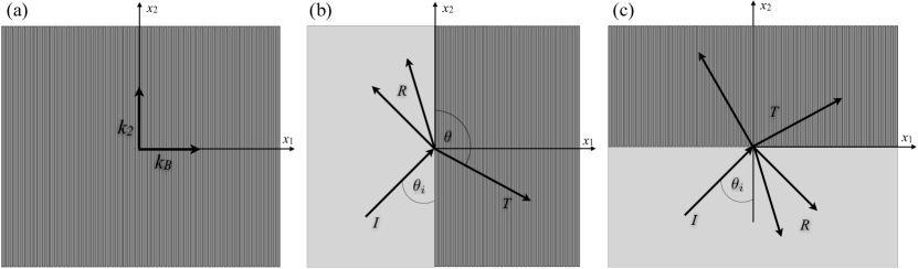
Figure 1: (a) An infinite laminate comprising alternating a and b phases. The medium admits Bloch modes with vertical wavenumber $k_{2}$, and macroscopic horizontal wavenumber $k_{\mathrm{B}}$. (b) A homogeneous half-space bonded to a semi-infinite laminate at $x_{1}=0$, and at (c) $x_{2}=0$. We schematically denote the incident, reflected and transmitted waves by $I,R$ and $T$, respectively. The incident and transmission angles are denoted by $\theta_{i}$ and $\theta$, respectively.

The objective is to determine the propagation of free time-harmonic in-plane waves in the laminate. To this end, we seek solutions for the displacements $u_{1}{}^{\left(n\right)}$ and $u_{2}{}^{\left(n\right)}$ in each $n^{\mathrm{th}}$ layer using the Naiver-Lamé equations

$$\begin{aligned} \left(\lambda{}^{\left(\emph{p}\right)}+2\mu{}^{\left(\emph{p}\right)}\right)u_{1,11}{}^{\left(n\right)}+\left(\lambda{}^{\left(\emph{p}\right)}+\mu{}^{\left(\emph{p}\right)}\right)u_{2,21}{}^{\left(n\right)}+\mu{}^{\left(\emph{p}\right)}u_{1,22}{}^{\left(n\right)}=\rho{}^{\left(\emph{p}\right)}\ddot{u_{1}}{}^{\left(n\right)},\\ \left(\lambda{}^{\left(\emph{p}\right)}+2\mu{}^{\left(\emph{p}\right)}\right)u_{2,22}{}^{\left(n\right)}+\left(\lambda{}^{\left(\emph{p}\right)}+\mu{}^{\left(\emph{p}\right)}\right)u_{1,12}{}^{\left(n\right)}+\mu{}^{\left(\emph{p}\right)}u_{2,11}{}^{\left(n\right)}=\rho{}^{\left(\emph{p}\right)}\ddot{u_{2}}{}^{\left(n\right)},\end{aligned}$$ (1)

subjected to boundary conditions that will be specified later. We employ the Helmholtz decomposition to write the in-plane components of $\bm{u}{}^{\left(n\right)}$ in terms of scalar potential $\phi{}^{\left(n\right)}$ and $\psi{}^{\left(n\right)}$, namely,

$$\begin{aligned} u_{1}{}^{\left(n\right)}=\phi_{,1}{}^{\left(n\right)}+\psi_{,2}{}^{\left(n\right)},\ \ &u_{2}{}^{\left(n\right)}=\phi_{,2}{}^{\left(n\right)}-\psi_{,1}{}^{\left(n\right)}\end{aligned}.$$ (2)

This decomposition simplifies Eq.  (1) to the form

$$\nabla^{2}\phi{}^{\left(n\right)}=\frac{1}{c_{L}^{2\left(\emph{p}\right)}}\ddot{\phi}{}^{\left(n\right)}, \nabla^{2}\psi{}^{\left(n\right)}=\frac{1}{c_{S}^{2\left(p\right)}}\ddot{\psi}{}^{\left(n\right)},$$ (3)

where $c_{L}^{\left(\emph{p}\right)}=\sqrt{\left(\lambda^{\left(p\right)}+2\mu^{\left(p\right)}\right)/\rho^{\left(p\right)}}$ and $c_{S}^{\left(\emph{p}\right)}=\sqrt{\mu^{\left(p\right)}/\rho^{\left(p\right)}}$ are the pressure and shear wave velocities of phase p, respectively. At a fixed frequency $\omega$, Eq. (3) is solved by

$$\phi{}^{\left(n\right)}=A_{L+}^{\left(\emph{n}\right)}e^{i\left(\omega t+k_{L}^{\left(\emph{p}\right)}x_{1}-k_{2}{}^{\left(\emph{p}\right)}x_{2}\right)}+A_{L-}^{\left(\emph{n}\right)}e^{i\left(\omega t-k_{L}^{\left(\emph{p}\right)}x_{1}-k_{2}{}^{\left(\emph{p}\right)}x_{2}\right)},$$ (4)

$$\psi{}^{\left(n\right)}=A_{S+}^{\left(\emph{n}\right)}e^{i\left(\omega t+k_{S}^{\left(p\right)}x_{1}-k_{2}{}^{\left(\emph{p}\right)}x_{2}\right)}+A_{S-}^{\left(\emph{n}\right)}e^{i\left(\omega t-k_{S}^{\left(p\right)}x_{1}-k_{2}{}^{\left(\emph{p}\right)}x_{2}\right)},$$

where

$$k_{L}^{2\left(\emph{p}\right)}=\frac{\omega^{2}}{c_{L}^{2\left(\emph{p}\right)}}-k_{2}^{2}{}^{\left(\emph{p}\right)}, k_{S}^{2\left(\emph{p}\right)}=\frac{\omega^{2}}{c_{S}^{2\left(\emph{p}\right)}}-k_{2}^{2}{}^{\left(\emph{p}\right)},$$ (5)

and $\left\{A_{L/S,\pm}{}^{\left(n\right)}\right\}$ are integration constants to be determined from the conditions on the boundaries of layer $n$. These correspond to the continuity of the traction and displacements at interfaces between adjacent layers, which immediately requires $k_{2}^{\left(\emph{a}\right)}=k_{2}^{\left(\emph{b}\right)}\eqqcolon k_{2}$. The corresponding equations are compactly written in terms of the state vector $\mathsf{s}{}^{\left(n\right)}\left(x_{1},x_{2},t\right)$

$$\mathsf{s}{}^{\left(n\right)}=\left(u_{1}{}^{\left(n\right)},\sigma_{11}{}^{\left(n\right)},u_{2}{}^{\left(n\right)},\sigma_{21}{}^{\left(n\right)}\right)^{\mathsf{T}};$$ (6)

say the boundary between layers $n$ and $n+1$ is at $x_{1}=x_{0}^{\left(n\right)}$, then the continuity conditions are simply $\mathsf{s}{}^{\left(n\right)}\left(x_{1}=x_{0}{}^{\left(n\right)}\right)=\mathsf{s}^{\left(n+1\right)}\left(x_{1}=x_{0}{}^{\left(n\right)}\right)$. The coupling between shear and pressure modes enters through the latter condition, since the components of $\mathsf{s}{}^{\left(n\right)}$ depend both on $\phi{}^{\left(n\right)}$ and $\psi{}^{\left(n\right)}$. The remaining equations stem from the Bloch-Floquet theorem, which states that over the course of one period the governing fields are related via the Bloch wavenumber $k_{\mathrm{B}}$, namely,

$$\mathsf{s}{}^{\left(n\right)}\left(x_{1}=x_{0}{}^{\left(n\right)}-h{}^{\left(n\right)}\right)=e^{ik_{\mathrm{B}}h}\mathsf{s}^{\left(n+1\right)}\left(x_{1}=x_{0}{}^{\left(n\right)}+h^{\left(n+1\right)}\right).$$ (7)

2.2 The hybrid matrix method to determine $k_{\mathrm{B}}\left(\omega\right)$

Eqs. (6) and (7) can be combined in different ways to deliver an eigenproblem for $k_{\mathrm{B}}$ and $\mathsf{s}{}^{\left(n\right)}$ as functions of real $\omega$ at prescribed $k_{2}$, given the laminate composition. The transfer matrix formulation is the most intuitive and common approach, however it suffers from numerical instabilities (Pérez-Álvarez et al., 2015). Here, we employ the stable hybrid matrix method (Tan, 2010), which reads

$$\left(\begin{array}[]{ll}-\mathsf{I}_{2}&\mathsf{H}_{11}\\ \mathsf{0}_{2}&\mathsf{H}_{21}\end{array}\right)\cdot\mathsf{s_{m}}\left(x_{1},x_{2}\right)=e^{ik_{B}h}\left(\begin{array}[]{ll}-\mathsf{H}_{12}&\mathsf{0}_{2}\\ -\mathsf{H}_{22}&\mathsf{I}_{2}\end{array}\right)\cdot\mathsf{s_{m}}\left(x_{1},x_{2}\right),$$ (8)

where $\mathsf{0}_{2}$ (resp. $\mathsf{I}_{2}$) is the $2\times 2$ zeros (resp. unit) matrix, and $\mathsf{s_{m}}$ and $\mathsf{H}_{ij}$ are given in Appendix A, together with a detailed derivation of Eq. (8). The resultant quartic equation for $k_{\mathrm{B}}$ is solved by

$$\cos k_{\mathrm{B}}h=\frac{-a_{2}\pm\sqrt{a_{2}^{2}-4a_{1}\left(a_{3}-2a_{1}\right)}}{4a_{1}},$$ (9)

where $a_{i}$ are given in Appendix A. Eq.  (9) provides the dispersion relation which relates the microstructure and mechanical properties of the laminate to the waveform at each frequency. The structure of Eq.  (9) implies that if $k_{\mathrm{B}}$ is a solution, then so are $\pm k_{\mathrm{B}}+2\pi m$ for any $m\in\mathbb{Z}$. Hence, the real part of all dispersion curves is representable over the irreducible $1^{\mathrm{st}}$ Brillouin zone $0<k_{\mathrm{B}}<\pi/h$. The wavenumber $k_{\mathrm{B}}$ can be real, pure imaginary (henceforth referred as imaginary) or complex, as demonstrated in the sequel, and contrary to the case of anti-plane shear (Willis, 2015, Srivastava, 2016). This property is essential for the spectrum to exhibit a Riemann structure, and, in turn, exceptional points. Real $k_{\mathrm{B}}$ corresponds to a propagating Bloch mode along $x_{1}$, where imaginary $k_{\mathrm{B}}$ corresponds to attenuating modes, with the exponential decay $e^{-\left|k_{\mathrm{B}}\right|x_{1}}$; since $e^{in\pi}=\pm 1$ for integer $n$, we will also refer to $k_{\mathrm{B}}$ with Re$\,k_{\mathrm{B}}h=n\pi$ as imaginary, and interpret corresponding modes as non-propagating. We note that modes with $k_{\mathrm{B}}h=n\pi$ are at the boundary of the Brillouin zones, and represent standing waves. Complex $k_{\mathrm{B}}$ describes a progressive mode that exponentially decay according to Im$\,k_{\mathrm{B}}$. We emphasize that wave attenuation is not an indication of energy loss, as our system is non-dissipative; it is the result of a gradual scattering of energy to incoherent waves with zero mean. Bands of frequencies without real $k_{\mathrm{B}}$ roots are termed directional band gaps (or simply gaps) since there is a gap in the spectrum in the $x_{1}$ direction. When there are no real $k_{2}$ solutions across these bands, they are termed complete gaps, since all directions of propagation are prohibited.

2.3 An eigenvalue problem for $k_{2}$ using a plane wave approach

The standard plane wave expansion method to obtain the dispersion relation in elastodynamics dates back to Sigalas and Economou (1992) and Kushwaha et al. (1993). In photonics, the method has been extended by Hsue et al. (2005) to a formulation in which the Bloch wavenumber is the eigenvalue, and later on by Laude et al. (2009) for elastodynamics. A general analysis of the method, associated linear operators, and the properties of the eigenvalues was carried out recently by Mokhtari et al. (2019). Building upon the approach of Laude et al. (2009), we formulate for our settings an eigenvalue problem in which $k_{2}$ is the eigenvalue. We begin by deriving the standard plane wave method by substituting into the Cauchy equations of motion

$$\left\{\left(u_{i,j}+u_{j,i}\right)\mu\left(x_{1}\right)+\lambda\left(x_{1}\right)\delta_{ij}u_{k,k}\right\}_{,j}=\rho\left(x_{1}\right)\ddot{u}_{i},$$ (10)

the Bloch form

$$u_{i}=\tilde{u}_{i}\left(x_{1}\right)e^{i\left(\omega t-k_{\mathrm{B}}x_{1}-k_{2}x_{2}\right)},\quad\tilde{u}_{i}\left(x_{1}\right)=\tilde{u}_{i}\left(x_{1}+h\right),$$ (11)

where here and henceforth, the periodic part of $\left(\circ\right)$ is denoted by $\tilde{\left(\circ\right)}$. Since $\rho\left(x_{1}\right)$, $\mu\left(x_{1}\right)$, $\lambda\left(x_{1}\right)$ and $\tilde{u}_{i}\left(x_{1}\right)$ are periodic in $x_{1}$ with a period $h$, they can be written as

$$\zeta\left(x_{1}\right)=\sum_{\mathrm{G}}\zeta\left(\mathrm{G}\right)e^{-i\mathrm{G}x_{1}},\ \ \ \zeta=\rho,\mu,\lambda,\tilde{u}_{1},\tilde{u}_{2},$$ (12)

where $\mathrm{G}=\frac{2\pi m}{h}$, $m\in\mathbb{Z}$, with the Fourier coefficients $\left\{\zeta\left(\mathrm{G}\right)\right\}$

$$\zeta\left(\mathrm{G}\right)=\frac{1}{h}\int_{0}^{h}\zeta\left(x_{1}\right)e^{i\mathrm{G}x_{1}}\mathrm{d}x_{1}.$$ (13)

We have that

$$\zeta\left(\mathrm{G}\right)=\begin{cases}\frac{h^{\left(\emph{a}\right)}}{h}\zeta^{\left(\emph{a}\right)}+\frac{h^{\left(\emph{b}\right)}}{h}\zeta^{\left(\emph{b}\right)},&\mathrm{G}=0,\\ \left(\pi m\right)^{-1}\left(\zeta^{\left(\emph{a}\right)}-\zeta^{\left(\emph{b}\right)}\right)\left(1-e^{i\mathrm{G}h^{\left(\emph{a}\right)}}\right),&\mathrm{G}\neq 0.\end{cases}$$ (14)

Substituting Eqs.  (11) and (12) into Eq. (10) and factoring out $e^{i\left(\omega t-k_{\mathrm{B}}x_{1}-k_{2}x_{2}\right)}$ yield

$$\begin{split}&\sum_{\mathrm{G},\mathrm{G^{\prime}}}\left\{-k_{2}\left[k_{2}\tilde{u}_{1}\left(\mathrm{G^{\prime}}\right)+\left(\mathrm{G^{\prime}}+k_{\mathrm{B}}\right)\tilde{u}_{2}\left(\mathrm{G^{\prime}}\right)\right]\mu\left(\mathrm{G}\right)\right.-\\ &-\left.\left(\mathrm{G}+\mathrm{G^{\prime}}+k_{\mathrm{B}}\right)\left[k_{2}\lambda\left(\mathrm{G}\right)\tilde{u}_{2}\left(\mathrm{G^{\prime}}\right)+\left(\mathrm{G^{\prime}}+k_{\mathrm{B}}\right)\left(\lambda\left(\mathrm{G}\right)+2\mu\left(\mathrm{G}\right)\right)\tilde{u}_{1}\left(\mathrm{G^{\prime}}\right)\right]\right\}e^{-i\left(\mathrm{G}+\mathrm{G^{\prime}}\right)x_{1}}=\\ &=-\sum_{\mathrm{G},\mathrm{G^{\prime}}}\omega^{2}\rho\left(\mathrm{G}\right)\tilde{u}_{1}\left(\mathrm{G^{\prime}}\right)e^{-i\left(\mathrm{G}+\mathrm{G^{\prime}}\right)x_{1}},\\ &\sum_{\mathrm{G},\mathrm{G^{\prime}}}\left\{-k_{2}\left[\left(\mathrm{G^{\prime}}+k_{\mathrm{B}}\right)\lambda\left(G\right)+\left(\mathrm{G}+\mathrm{G^{\prime}}+k_{\mathrm{B}}\right)\mu\left(\mathrm{G}\right)\right]\tilde{u}_{1}\left(\mathrm{G^{\prime}}\right)-k_{2}^{2}\lambda\left(\mathrm{G}\right)\tilde{u}_{2}\left(\mathrm{G^{\prime}}\right)\right.-\\ &-\left.\mu\left(\mathrm{G}\right)\left[2k_{2}^{2}+\left(\mathrm{G^{\prime}}+k_{\mathrm{B}}\right)\left(G+\mathrm{G^{\prime}}+k_{\mathrm{B}}\right)\right]\tilde{u}_{2}\left(\mathrm{G^{\prime}}\right)\right\}e^{-i\left(\mathrm{G}+\mathrm{G^{\prime}}\right)x_{1}}=\\ &=-\sum_{\mathrm{G},\mathrm{G^{\prime}}}\omega^{2}\rho\left(\mathrm{G}\right)\tilde{u}_{2}\left(\mathrm{G^{\prime}}\right)e^{-i\left(\mathrm{G}+\mathrm{G^{\prime}}\right)x_{1}}.\end{split}$$ (15)

We multiply Eqs. (15) by $e^{i\mathrm{G^{\prime\prime}}x_{1}}$ and integrate over one period. Due to Fourier orthogonality, only terms satisfying $\mathrm{G^{\prime\prime}}=\mathrm{G}+\mathrm{G^{\prime}}$ remain, and we end up with an infinite set of equations that can be cast in matrix form as

$$\left[\mathsf{A}_{0}+k_{2}\mathsf{A}_{1}+k_{2}^{2}\mathsf{A}_{2}\right]\mathsf{\tilde{u}}\left(\mathrm{G^{\prime}}\right)=\omega^{2}\mathsf{B}\mathsf{\tilde{u}}\left(\mathrm{G^{\prime}}\right),$$ (16)

where $\mathsf{\tilde{u}}\left(\mathrm{G^{\prime}}\right)$ is a column vector comprising the Fourier coefficients of $\tilde{u}_{1}$ and $\tilde{u}_{2}$, and the matrices $\mathsf{A}_{0},\mathsf{A}_{1},\mathsf{A}_{2}$ and $\mathsf{B}$ are given in Appendix B. Eq.  (16) constitutes a generalized eigenproblem for $\omega^{2}$ and $\mathsf{\tilde{u}}\left(\mathrm{G^{\prime}}\right)$ at prescribed $k_{2}$ and $k_{\mathrm{B}}$. A mixed generalized eigenproblem for $k_{2}$ at prescribed $\omega$ and $k_{\mathrm{B}}$ follows from Eq.  (16) using a state space-like formulation (Chapt.  10 in Deymier, 2013, see also Hussein et al., 2014), namely,

$$\left[\begin{array}[]{ll}\mathsf{0}&\mathsf{I}\\ \omega^{2}\mathsf{B}-\mathsf{A}_{0}&-\mathsf{A}_{1}\end{array}\right]\left(\begin{array}[]{l}\mathsf{\tilde{u}}\left(\mathrm{G^{\prime}}\right)\\ k_{2}\mathsf{\tilde{u}}\left(\mathrm{G^{\prime}}\right)\end{array}\right)=k_{2}\left[\begin{array}[]{ll}\mathsf{I}&\mathsf{0}\\ \mathsf{0}&\mathsf{A}_{2}\end{array}\right]\left(\begin{array}[]{l}\mathsf{\tilde{u}}\left(\mathrm{G^{\prime}}\right)\\ k_{2}\mathsf{\tilde{u}}\left(\mathrm{G^{\prime}}\right)\end{array}\right)$$ (17)

For completeness, note that an equivalent formulation can be obtained using the displacement together with the stress and the eigenvector (Mokhtari et al., 2019). For computational purposes, the number of terms in the Fourier series is truncated, say by $-N\leq m\leq N$. The matrices $\mathsf{A}_{i},\mathsf{B},\mathsf{0}$ and $\mathsf{I}$ are accordingly of dimension $\left(2N+1\right)\times\left(2N+1\right)$.

2.4 Some properties of $k_{\mathrm{B}}$ and $k_{2}$ and their effect on energy transport

To highlight how the coupling between shear and pressure waves affect $k_{\mathrm{B}}$ and $k_{2}$, we record next their properties in the case of anti-plane shear in laminates, where such coupling is absent, and subsequently point out the differences. These differences have significant implications on frequency spectrum, and in turn the energy flow, since the slopes of propagating branches are a measure of its mean. More formally, the average energy flow is

$$\left\langle\bm{\mathcal{P}}\right\rangle=-\frac{1}{2}\left\langle\mathrm{Re}\left[\bm{\sigma}\dot{\bm{u}}^{*}\right]\right\rangle,$$ (18)

and satisfies (Willis, 2015)

$$\left\langle\bm{\mathcal{P}}\right\rangle=\frac{\partial\omega}{\partial\bm{k}}E,\quad E=\frac{1}{4}\left\langle\sigma_{ij}u_{i,j}^{*}\right\rangle+\frac{1}{4}\omega^{2}\left\langle\rho u_{k}^{*}u_{k}\right\rangle\equiv\frac{1}{2}\omega^{2}\left\langle\rho u_{k}^{*}u_{k}\right\rangle,$$ (19)

where $\left\langle\circ\right\rangle$ denotes averaging over one spatial and temporal period, and $E$ is the total mean energy density; $\bm{\mathcal{P}}$ is called the acoustic Poynting vector, and the $\bm{k}$-gradient of $\omega$ is identified as the group velocity.

Exceptional points.—In anti-plane shear, the size of the transfer matrix is $2\times 2$, whose two roots are $\lambda_{1,2}=e^{ik_{B1,B2}h}$. When the transfer matrix is real, one can show that if $\lambda$ is a solution, then so are $\lambda^{*}$ and $\lambda^{-1}$ . Since there are only two roots, either $\lambda=\lambda^{*}$ and then $k_{\mathrm{B}}$ is imaginary, or $\lambda^{*}=\lambda^{-1}$ and then $k_{\mathrm{B}}$ is real. Accordingly, eigenvalue degeneracies occur only at the edge of the irreducible Brillouin zones, where the modes are standing and not propagating. In this usual degeneracy, the eigenmodes remain linearly independent, and the splitting of the eigenvalues from the so-called diabolic points scales linearly.

The situation is significantly different when there are two coupled displacements as considered here. The size of the corresponding transfer matrix is $4\times 4$, thus has four roots. Hence, the fact that $\lambda^{*}$ and $\lambda^{-1}$ are also solutions does not enforce that $\lambda=\lambda^{*}$ or $\lambda^{*}=\lambda^{-1}$, and, in turn the exclusion of complex $k_{\mathrm{B}}$ roots. As we show in Sec. 3, not only such complex roots exist, they coalesce together with their eigenmodes at exceptional points inside the irreducible $1^{\mathrm{st}}$ Brillouin zone, according to a square-root scaling, constituting a Riemann surface structure.

Negative refraction.—We quantify the flow direction of each mode that is propagating in the laminate plane using the angle (Fig.  1)

$$\theta=\arctan\frac{\left\langle\mathcal{P}_{1}\right\rangle}{\left\langle\mathcal{P}_{2}\right\rangle}=\arctan\frac{\partial\omega/\partial k_{\mathrm{B}}}{\partial\omega/\partial k_{2}}.$$ (20)

Srivastava (2016) showed analytically for anti-plane shear waves that $k_{2}$ and $\mathcal{P}_{2}$ share the same sign, and hence so does $\left\langle\mathcal{P}_{2}\right\rangle$. Therefore, the macroscopic transport of energy of anti-plane shear waves in the $x_{2}$ direction is aligned with the local transport. This implies that in the canonical configuration of excitation (Joseph and Craster, 2015), i.e., when the laminate is impinged by a wave at a boundary normal to the lamination direction (Fig. 1b), anti-plane shear will always refract positively. The reason is that continuity requires the excited Bloch waves to share the same vertical wavenumber as the incident wave, and hence the incident angle and the angle of the Bloch waves have the same sign. In the present problem, where $\mathcal{P}_{2}$ is

$$\mathcal{P}_{2}=\frac{1}{2}\omega\mathrm{Re}\left\{\mu\left(k_{2}\tilde{u}_{1}+k_{\mathrm{B}}\tilde{u}_{2}+i\tilde{u}^{\prime}_{2}\right)\tilde{u}_{1}^{*}+\left(k_{\mathrm{B}}\lambda\tilde{u}_{1}+k_{2}\left(\lambda+2\mu\right)\tilde{u}_{2}+i\lambda\tilde{u}^{\prime}_{1}\right)\tilde{u}_{2}^{*}\right\},\ \left(\cdot\right)^{\prime}\equiv\frac{\partial\left(\cdot\right)}{\partial x_{1}},$$ (21)

this is no longer the case; as we will demonstrate in the sequel, there are positive $k_{2}$ for which simultaneously $\left\langle\mathcal{P}_{2}\right\rangle<0$ and $\left\langle\mathcal{P}_{1}\right\rangle>0$, where

$$\mathcal{P}_{1}=\frac{1}{2}\omega\mathrm{Re}\left\{\mu\left(k_{2}\tilde{u}_{1}+k_{\mathrm{B}}\tilde{u}_{2}+i\tilde{u}^{\prime}_{2}\right)\tilde{u}_{2}^{*}+\left(\lambda+2\mu\right)\left(k_{\mathrm{B}}\tilde{u}_{1}+i\tilde{u}^{\prime}_{1}\right)\tilde{u}_{1}^{*}+\lambda k_{2}\tilde{u}_{2}\tilde{u}_{1}^{*}\right\}.$$ (22)

This implies that negative refraction is realizable in the simple interface configuration.

Willis (2015) devised a complex configuration to achieve negative refraction of anti-plane shear waves, by considering waves impinging at an interface parallel to the lamination direction (Fig. 1c). We will additionally show that in-plane waves can refract negatively in this excitation setup as well.

3 Mode spectrum of an exemplary laminate

In this Sec., we study the frequency spectrum of in-plane waves propagating through an infinite laminate comprising steel and acrylic layers, whose properties are

$$\begin{array}[]{ll}\mu^{\left(1\right)}=78.85\,\mathrm{GPa},\lambda^{\left(1\right)}=118.27\,\mathrm{GPa},&\rho^{\left(1\right)}=7800\,\mathrm{kg\,m^{-3}},h^{\left(1\right)}=1.3\,\mathrm{mm},\\ \mu^{\left(2\right)}=1.21\,\mathrm{GPa},\ \lambda^{\left(2\right)}=4.86\,\mathrm{GPa},&\rho^{\left(2\right)}=1200\,\mathrm{kg\,m^{-3}},h^{\left(2\right)}=3\,\mathrm{mm}.\end{array}$$ (23)

The same laminate was considered by Nemat-Nasser (2015), Willis (2015) and Srivastava (2016) to study anti-plane shear waves. The forthcoming study of the spectrum is the basis for the transmission analysis in Sec.  4. To simplify the presentation of the spectrum, we fix one of the three parameters $\left\{\omega,\ k_{\mathrm{B}},\ k_{2}\right\}$, and evaluate the relation between the remaining two.

[figure]style=plain,subcapbesideposition=top

[]  []  []

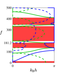
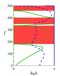
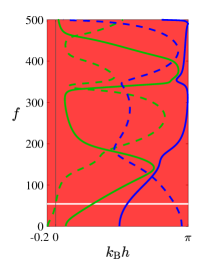
Figure 2: The ordinary frequency $f$ (in $\mathrm{kHz}$) versus $k_{\mathrm{B}}h$ restricted to $0<k_{\mathrm{B}}h<\pi$ for laminate (23) at (a) $k_{2}h=0.5$, (b) $0.5i$, and (c) $0.5+0.5i$. Re$\,k_{\mathrm{B}}h$ and |Im$\,k_{\mathrm{B}}h$| (Im$\,k_{\mathrm{B}}$ in panel c) are shown in solid and dashed curves, respectively. The real and imaginary parts of a certain branch are plotted using the same color. Gaps are indicated by the red shading.

Our analysis begins by plotting in Fig. 2 the ordinary frequency $f=\omega/2\pi$ versus $0<k_{\mathrm{B}}h<\pi$ at prescribed $k_{2}$ values. Panels 2(a)-(c) correspond to $k_{2}h=0.5,\ 0.5i,$ and $0.5+0.5i$, respectively. Re$\,k_{\mathrm{B}}h$ and |Im$\,k_{\mathrm{B}}h$| (Im$\,k_{\mathrm{B}}h$ in panel c) are shown in solid and dashed curves, respectively, where the real and imaginary parts of a certain branch are plotted using the same color. Gaps are indicated by the red shading.

Panel 2(a) exhibits the following notable features. Firstly, there are no branches with real $k_{\mathrm{B}}$ from $f=0$ to $14.1\,\mathrm{kHz}$. In a study of the dependency of this gap on Re$\,k_{2}h$ (not shown here), we found that it widens as Re$\,k_{2}h$ increases. Across $136.2<f<181.2\ \mathrm{kHz}$, the branches are complex conjugates of each other; from $f=159.3\ \mathrm{kHz}$ the imaginary parts decrease until they vanish at $f\approx 181.2\ \mathrm{kHz}$. At this exceptional point the eigenvalues coalesce. Beyond this point there is a special narrow range where both branches are real, while their slopes have an opposite sign, i.e., the modes are propagating in opposite directions; this is the fingerprint of exceptional points.

Panel 2(b) exhibits different characteristics. Firstly, across the studied frequencies, one of the branches always has an imaginary part, hence the maximal number of modes that propagate in $x_{1}$ at any frequency is one. Contrary to the case in panel 2(a), here the first gap emerges above $f=0$, namely, at $f=180.6\ \mathrm{kHz}$. In a study of the dependency of this gap on Im$\,k_{2}h$ (not shown here), we found that gaps starting at $f=0$ emerge at higher values of Im$\,k_{2}h$. Thus, the diagram starts with a propagating band, where the horizontal group velocity changes sign at $f=148\ \mathrm{kHz}$. This flip of sign inside the irreducible first Brillouin zone is unique to in-plane waves.

Panel 2(c) shows an anomalous scenario without passbands, except at a discrete frequency ($f\approx 54.2\,$kHz) for which one branch is propagating. To facilitate the visual identification of this frequency, here we plot the signed imaginary part instead of its absolute value. Accordingly, this frequency is spotted by the zero crossing of Im$\,k_{\mathrm{B}}h$. There is no counterpart to this phenomenon in anti-plane waves, where complex $k_{2}$ are not accessible.

[figure]style=plain,subcapbesideposition=top

[]  []

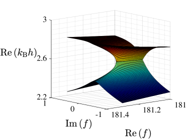
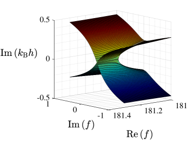
Figure 3: The (a) real and (b) imaginary part of $k_{\mathrm{B}}h$ versus the real and imaginary parts of $f$, for $k_{2}h=0.5$.

Fig. 3 shows the (a) real and (b) imaginary parts of $k_{\mathrm{B}}h$ as functions of $f$ at $k_{2}h=0.5$, when we carry out an analytic continuation to the dispersion relation, such that the domain of the spectrum is formally extended to complex-valued frequencies. We emphasize that here, this is an artificial continuation (see, e.g., Shanin et al., 2018), as complex frequencies are not accessible (we are concerned with time-harmonic waves in a system with no dissipation). Lu and Srivastava (2018), for example, considered an analytic continuation of the shear modulus, which has the physical interpretation of a system with gain or loss.

The spectrum exhibits a structure of a Riemann surface in the vicinity of the exceptional point: Fig. 2(a) is thus a section of that surface, at the plane Im$\,f=0$. In view of the duality of between the frequency and the wavenumbers (Torrent et al., 2018) in the different forms of the eigenvalue problem (Mokhtari et al., 2019), a Riemann surface is expected when $f$ is fixed and the roots of $k_{\mathrm{B}}$ are evaluated against $k_{2}$, as we will demonstrate in the sequel. Importantly, the states of the system in the complex wave vector space are accessible, and are not merely a formal extension.

[figure]style=plain,subcapbesideposition=top

[]  []

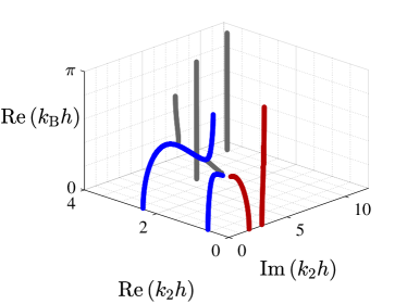
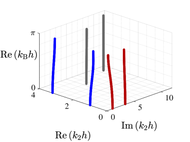
Figure 4: Pure real $k_{\mathrm{B}}h$ branches as function of the real and imaginary parts of $k_{2}h$ for laminate (23) at (a) $f=100\ \mathrm{kHz}$, and (b) $160\ \mathrm{kHz}$. Segments of real, imaginary and complex $k_{2}$ are denoted by blue, red, and grey, respectively.

Towards this end, we fix $f$ and examine the spectrum in the complex $k_{\mathrm{B}}-k_{2}$ space. Figs. 4(a) and 4(b) show branches of purely real $k_{\mathrm{B}}$ versus Re$\,k_{2}h$ and Im$\,k_{2}h$, at $f=100\ \mathrm{kHz}$ and $160\ \mathrm{kHz}$, respectively. Segments of real, imaginary and complex $k_{2}$ are denoted by blue, red, and grey, respectively. Notably, the number of modes with real or imaginary $k_{2}$ is finite. In our study (not shown here) the number of modes with real or imaginary $k_{2}$ increases with the frequency. We further note that in our study on branches with complex $k_{2}$, we found that their number is infinite, although it cannot be observed from the truncated diagram we show. By contrast, Srivastava (2016) showed that in the anti-plane motion there are no complex $k_{2}$, and the number of branches with imaginary $k_{2}$ is infinite. In both cases (anti-plane and in-plane waves), the existence of an infinite number of decaying modes conforms with the need of such a set in satisfying the continuity of the displacement and traction across certain interfaces (Srivastava and Willis, 2017). [figure]style=plain,subcapbesideposition=top

[]  []  []  []  []  []

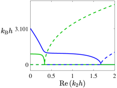
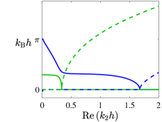
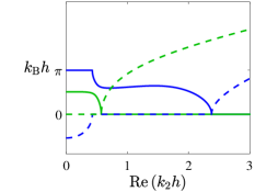
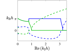
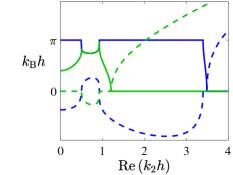
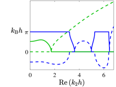
Figure 5: The real (solid curves) and imaginary (dashed curves) parts of $k_{\mathrm{B}}h$ as functions of Re$\,k_{2}h$ for laminate (23), at Im$\,k_{2}h=0$ and (a) $f=60$, (b) $60.1$, (c) $100$, (d) $160$, (e) $181.3$, and (f) $340\,\mathrm{kHz}$. Parts of the same branch are plotted using the same color.

Modes that propagate along both $x_{1}$ and $x_{2}$ are studied in Fig. 5, by restricting attention to the plane Im$\,k_{2}h=0$, and evaluating $k_{\mathrm{B}}h$ versus Re$\,k_{2}h$ at prescribed frequencies. The real and imaginary parts of $k_{\mathrm{B}}$ are shown in solid and dashed curves, respectively, where each color corresponds to a different branch.

At $f=60\ \mathrm{kHz}$ (panel 5a), two modes of different branches are propagating when $0<k_{\mathrm{B}}h<0.919$; only one mode propagates when $0.919<k_{\mathrm{B}}h<3.101$, and at larger Bloch wavenumbers there are no propagating modes. Here and at higher frequencies, we find that beyond the illustrated $k_{2}$-interval there are no propagating branches—solutions at higher $k_{2}$ values are always given by $k_{\mathrm{B}}$ with an imaginary part, such that $k_{\mathrm{B}}$ is either imaginary or complex.

At a slightly higher frequency ($f=60.1\ \mathrm{kHz}$, panel 5b), the whole $1^{\mathrm{st}}$ Brillouin zone admits real solutions, contrary to the case at $f=60\ \mathrm{kHz}$. This change in the spectrum between the frequencies has a significant implication on beam steering, as we will show in Sec. 4.2. In a narrow range near $k_{2}h=0$, the blue mode has a non-zero imaginary part and its real part equals $\pi$. Thus, for the frequencies in panels 5(a)-(b) and displayed range of $k_{2}h$ values, the Bloch wavenumber of the modes is either real, or has an imaginary part with Re$\,k_{\mathrm{B}}h=0$ mod $\pi$.

Panel 5(c), which evaluates the modes at $f=100\ \mathrm{kHz}$, also shares the latter characteristic. Here, however, the real part of the blue is a non-monotonic function of $k_{2}h$, as it changes trend twice. This is the fingerprint of an exceptional point, and an indicator of negative refraction as will be demonstrated in Sec. 4.2. Similarly to the observation made regarding the modes near the exceptional point in Fig. 2, the slopes of the two modes have different sign. There are accordingly three propagating modes across the range $1.87\apprle k_{\mathrm{B}}h\lesssim 2.03$ associated with the same branch, which exhibit different vertical wavelengths. These features are unique to the in-plane motion, as in the anti-plane motion the real part of $k_{\mathrm{B}}h$ is either monotonically increasing to $\pi$ or monotonically decreasing to $0$ (Srivastava, 2016).

At $f=160\ \mathrm{kHz}$ (panel 5d) across the interval $0<\mathrm{Re}\,k_{2}h\lesssim 0.79$, there are two complex conjugate pairs of $k_{\mathrm{B}}$ solutions with and identical real part, up to $k_{2}h\approx 0.79$. At this exceptional point, the imaginary part of all the branches vanishes, and the modes coalesce. Beyond this point, the real part of the branches diverges in a different directions, similarly to the feature observed in Fig. 2(a). At $k_{2}h\approx 0.8$, the blue branch becomes attenuating, and at $k_{2}h\approx 1$ the green branch also becomes imaginary. The blue mode is propagating again for $3.08<k_{2}h<3.22$; beyond that range there no more propagating modes.

When $f=181.3\,\mathrm{kHz}$ (panel 5e), there are two exceptional points at $k_{2}h=0.503$ and $0.93$. Again, in the vicinity of these points there are modes with slopes of different sign. As in panel 2(d), there is a range of Bloch wavenumbers with three propagating modes when $k_{\mathrm{B}}h>1.26$, where for lower $k_{\mathrm{B}}h$ there are two propagating modes.

We recall that in Fig.  2(a), we exhibited an exceptional point for $f=181.2\,\mathrm{kHz}$ and $k_{2}h=0.5$, i.e., when perturbing one of the parameters of the system about this point (e.g., $k_{2}h$ is perturbed from 0.5 to 0.503), another exceptional point emerges at a variation of another parameter of the system (e.g., is perturbed $f$ from 181.2 to $181.3\,\mathrm{kHz}$). This is not accidental; in fact, the exceptional points we demonstrate for each set of parameters comprise exceptional curves in a higher dimensional space.

At $f=340\,\mathrm{kHz}$ (panel 5f), the propagating green mode is a non-monotonic function of $k_{2}$, where initially it has a positive slope up to a maximal point, beyond which the slope changes sign, until the mode becomes imaginary at $k_{2}h=1.72$. The blue mode is either real or imaginary with $\mathrm{Re}\,k_{\mathrm{B}}h$ mod $\pi=0$. The number of propagating modes for prescribed $k_{\mathrm{B}}$ is higher than at lower frequencies, namely, a minimal number of three and a maximal number of five across $1.624<k_{\mathrm{B}}h<1.88$.[figure]style=plain,subcapbesideposition=top

[]  []

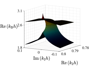
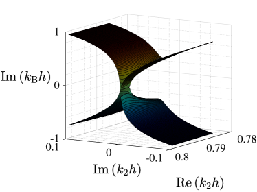
Figure 6: The (a) real and (b) imaginary parts of $k_{\mathrm{B}}h$ as functions of Re$\,k_{2}h$ and Im$\,k_{2}h$, at $f=160\,$kHz.

As mentioned earlier, we expect the spectrum to exhibit the structure of a Riemann surface near exceptional points in the complex $k_{\mathrm{B}}-k_{2}$ space. This is shown in Fig. 6, where the (a) real and (b) imaginary parts of $k_{\mathrm{B}}h$ are plotted against Re$\,k_{2}h$ and Im$\,k_{2}h$, at $f=160\,$kHz: Fig. 5(d) is thus the section Im$\,k_{2}=0$ of this surface. We emphasize again the the states of the system over this manifold are accessible since they correspond to realizable wavenumbers, and are not merely a formal extension.

[figure]style=plain,subcapbesideposition=top

[]  []  []

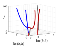
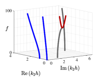
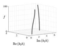
Figure 7: The ordinary frequency $f$ (in $\mathrm{kHz}$) versus real and imaginary parts of $k_{2}h$ solutions for laminate (23) at (a) $k_{\mathrm{B}}h=0.5$, (b) $0.5i$, and (c) $0.5+0.5i$. Segments of real, imaginary and complex $k_{2}$ are denoted by blue, red, and grey, respectively.

Finally, in Fig. 7 we fix $k_{\mathrm{B}}h$ and evaluate the spectrum in the $f-k_{2}$ space. Specifically, panels  7(a)-(c) correspond to $k_{\mathrm{B}}h=0.5,\,0.5i$ and $0.5+0.5i$, respectively; segments of real, imaginary and complex $k_{2}$ are denoted by blue, red, and grey, respectively. We observe that the number of modes in general—and propagating in particular—increases with frequency.

In panel 7(a) we observe an exceptional point when $k_{2}h=0.9i$ at 13 kHz, where a single complex mode branches to two imaginary modes; as frequency increases to 33 kHz, one of these branches becomes a propagating mode. A similar exceptional point is identified in panel 7(b), when $k_{2}h=2.3i$ at $72\,$kHz. There are no propagating modes in panel 7(c).

4 Transmission across an interface of a semi-infinite laminate

As mentioned, modes with either prescribed $k_{\mathrm{B}}$ or prescribed $k_{2}$ are excitable through two different configurations. We analyze the transmission and excited modes in these configurations, linking them to the exceptional points, negative refraction, and beam steering found in the spectrum, as reported in Sec.  3.

4.1 Metamaterial refraction via an interface parallel to the layers

To excite modes with designated vertical lengths, we connect the laminate at $x_{1}=0$ to a homogeneous half-space whose properties are denoted by the script 0, from which an incident wave propagates in an angle $\theta_{i}$ towards the interface (Fig. 1b). The wave is described by the potential $V$

$$V=Ie^{i\left(\omega t-k\sin\theta_{i}x_{1}-k\cos\theta_{i}x_{2}\right)},$$ (24)

where the wavenumber $k=\omega/c^{\left(0\right)}$ is either $\omega/c^{\left(0\right)}_{S}$ for a shear wave, or $\omega/c_{L}^{\left(0\right)}$ for a pressure wave. The incident displacements are derived according to Eq. (2), by setting $\psi^{\left(0\right)}=V$ for incident shear, or $\phi^{\left(0\right)}=V$ for incident pressure wave. The incident wave is partially reflected back by the interface, and partially transmitted to the laminate as Bloch modes. The continuity conditions at $x_{1}=0$ enforces all these waves to have an $x_{2}$-dependency in the form $e^{-ik\cos\theta_{i}x_{2}}$. Corresponding Bloch modes are extracted by the procedure in Sec. 2.1 with $k_{2}=k\cos\theta_{i}$, in the form

$$\mathbf{T}=\sum_{m=1}^{2}T_{m}\bm{\tilde{u}}^{\left(m\right)}\left(x_{1}\right)e^{i\left(\omega t-k_{\mathrm{B}}x_{1}-k\cos\theta_{i}x_{2}\right)},$$ (25)

where the reflected waves are derived from

$$\phi_{R}^{\left(0\right)}=R^{\phi}e^{i\left(\omega t+k_{L}^{\left(0\right)}x_{1}-k\cos\theta_{i}x_{2}\right)},\ \psi_{R}^{\left(0\right)}=R^{\psi}e^{i\left(\omega t+k_{S}^{\left(0\right)}x_{1}-k\cos\theta_{i}x_{2}\right)},$$ (26)

such that $k_{L}^{\left(0\right)}$ and $k_{S}^{\left(0\right)}$ are related to $k_{2}=k\cos\theta_{i}$ via Eq. (5). Finally, the reflection coefficients $R_{l}^{\phi},R_{l}^{\psi}$ and transmission coefficients $T_{m}$ are determined from the continuity of the state vector at $x_{1}=0$.

We numerically demonstrate how negative refraction is obtained, using a half-space with the properties

$$\mu^{\left(0\right)}=0.178\,\mathrm{GPa},\ \lambda^{\left(0\right)}=0.714\,\mathrm{GPa},\ \rho^{\left(0\right)}=3000\,\mathrm{kg/m^{3}}.$$ (27)

We set an incident pressure wave at $\theta_{i}=77.22^{\circ}$ and $f=100\,\mathrm{kHz}$, for which $k_{2}h=1$. The resultant Bloch wavenumbers are extractable from Fig. 5, where at the pertinent $k_{2}$ there is one attenuating mode and one propagating mode. We recall that the slope in Fig. 5 of the propagating mode at this $k_{2}$ is positive, while at higher $k_{2}$ the slope is negative, which is an indicator of negative refraction. This is verified by evaluating Eqs. (21)-(22), to find that the propagating angle is $\theta=107.03{}^{\circ}$. As a consistency check, we examine the balance of energy at $x_{1}=0$, namely,

$$\frac{1}{\left|I\right|^{2}\left\langle\mathcal{P}_{1}\right\rangle_{I}}\left[\sum_{m=1}^{2}\left|T_{m}\right|^{2}\left\langle\mathcal{P}_{1}\right\rangle_{T_{m}}^{\left(1\right)}-\left|R^{\phi}\right|^{2}\left\langle\mathcal{P}_{1}\right\rangle_{\phi}-\left|R^{\psi}\right|^{2}\left\langle\mathcal{P}_{1}\right\rangle_{\psi}\right]=1,$$ (28)

where the scripts $T_{m},\ \phi,\ \psi$ and $I$ denote quantities associated with the corresponding fields. Indeed, we find that the terms in left hand side are $0.617,\ 0.316$ and $0.067$, respectively, which sum to $1$. Note that only the propagating mode contributes to the first term, since the energy flux of the mode with the imaginary $k_{\mathrm{B}}$ vanishes.

As a second example, we set an incident shear incident wave at $\theta_{i}=89.62{}^{\circ}$ and $f=340\,\mathrm{kHz}$, for which $k_{2}h=0.25$. The resultant Bloch wavenumbers are extractable from Fig.  5(f). Here again, at the prescribed $k_{2}$ there is one attenuating mode, and one propagating mode with a positive slope, that will change sign at greater $k_{2}$. Calculation of Eqs. (21)-(22) confirms a negative refraction at $\theta=106.2^{\circ}$. Energy balance is also verified, where the calculation of the terms in the left hand side of Eq. (28) provides $0.148,\ 0.007$ and $0.845$, respectively, which again sum to $1$.

Fig.  8 shows frequency domain finite element simulations using COMSOL Multiphysics^® the energy flux along $x_{2}$ ($\mathcal{P}_{2}$) resulting from an (a) incident pressure wave at $\theta_{i}=77.22^{\circ}$ and $f=100\,\mathrm{kHz}$, and (b) an incident shear incident wave at $\theta_{i}=89.62{}^{\circ}$ and $f=340\,\mathrm{kHz}$. We used low reflecting boundary conditions to avoid reflections due to the finite truncation of the spatial domain. The incident wave was excited using load control over a defined line. We used triangular elements, whose maximal size was third of the unit-cell thickness. Indeed, the resultant negative angles of refraction agree with the analytical prediction.

[figure]style=plain,subcapbesideposition=top

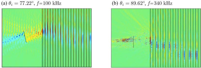
Figure 8: Frequency domain finite element simulations using COMSOL Multiphysics^® of the energy flux along $x_{2}$ ($\mathcal{P}_{2}$) resulting from an (a) incident pressure wave at $\theta_{i}=77.22^{\circ}$ and $f=100\,\mathrm{kHz}$, and (b) an incident shear incident wave at $\theta_{i}=89.62{}^{\circ}$ and $f=340\,\mathrm{kHz}$. The obtained negative angles of refraction agree with the analytical prediction.

4.2 Negative refraction via an interface normal to the layers

It is possible to excite designated Bloch wavenumbers using an incident wave from a homogeneous half-space that is bonded to the laminate by an interface along the lamination direction, say at $x_{2}=0$ (Fig. 1c). This configuration was proposed by Willis (2013) to achieve negative refraction of anti-plane shear waves, and was studied in greater detail by Willis (2015), Nemat-Nasser (2015), Srivastava (2016), and Morini et al. (2019). We recall that in this setup, an incident wave will excite an infinite number of decaying waves in the laminate, required to enforce continuity conditions (Srivastava and Willis, 2017). Here, we firstly develop a method to resolve the normal mode decomposition and energy partition of the excited in-plane waves in this configuration.

Consider again an incident wave according to the potential (24), now impinging on the horizontal interface $x_{2}=0$. In this setting, the continuity conditions at the interface enforce the reflected and transmitted waves to share the same horizontal length with the incident wave. Accordingly, the transmitted waves have the form

$$\mathbf{T}=\sum_{m=1}^{\infty}T_{m}\bm{\tilde{u}}^{\left(m\right)}\left(x_{1}\right)e^{i\left(\omega t-k_{\mathrm{B}}x_{1}-k_{m}x_{2}\right)},$$ (29)

where $k_{\mathrm{B}}=k\sin\theta_{i}$, and $\left\{k_{m}\right\}$ are extractable from Eq. (17). In view of the foregoing observations, the reflected waves is constructible from potentials that must have the form

$$\phi_{R}=\sum_{l=-\infty}^{\infty}R_{l}^{\phi}U_{l}\left(x_{1}\right)e^{i\left(\omega t-k_{\mathrm{B}}x_{1}+\kappa_{l}^{\phi}x_{2}\right)},\ \psi_{R}=\sum_{l=-\infty}^{\infty}R_{l}^{\psi}U_{l}\left(x_{1}\right)e^{i\left(\omega t-k_{\mathrm{B}}x_{1}+\kappa_{l}^{\psi}x_{2}\right)},$$ (30)

where

$$\kappa_{l}^{\phi}=\sqrt{\left(\omega/c^{\left(0\right)}_{L}\right)^{2}-\left(k\sin\theta+2\pi l/h\right)^{2}},\ \kappa_{l}^{\psi}=\sqrt{\left(\omega/c^{\left(0\right)}_{S}\right)^{2}-\left(k\sin\theta+2\pi l/h\right)^{2}},$$ (31)

and $U_{l}\left(x_{1}\right)=e^{-2l\pi ix_{1}/h}$.

The transmission and reflection coefficients $\left\{T_{m},R_{l}^{\phi},R_{l}^{\psi}\right\}$ are determined by the continuity conditions at $x_{2}=0$, which are compactly written as

$$\sum_{m=1}^{\infty}T_{m}\mathsf{s}_{T}^{\perp}{}^{\left(m\right)}-\sum_{l=-\infty}^{\infty}R_{l}^{\phi}\mathsf{s}_{\phi}^{\perp}{}^{\left(l\right)}-\sum_{l=-\infty}^{\infty}R_{l}^{\psi}\mathsf{s}_{\psi}^{\perp}{}^{\left(l\right)}=I\mathsf{s}_{I}^{\perp},$$ (32)

using

$$\mathsf{s}^{\perp}{}^{\left(n\right)}=\left(\tilde{u}_{1}{}^{\left(n\right)},\tilde{u}_{2}{}^{\left(n\right)},\tilde{\sigma}_{21}{}^{\left(n\right)},\tilde{\sigma}_{22}{}^{\left(n\right)}\right)^{\mathsf{T}}.$$ (33)

For computational purposes, we truncate the sums over $l$ and $m$ such that $-N_{R}\leq l\leq N_{R}$ and $1\leq m\leq 2\left(2N_{R}+1\right)$, and apply the elegant orthogonality relation (Mokhtari et al., 2019)

$$\int_{0}^{h}\left[\mathsf{s}_{1}^{\perp}{}^{\left(\beta\right)}\mathsf{s}_{3}^{\perp}{}^{*}{}^{\left(\alpha\right)}+\mathsf{s}_{2}^{\perp}{}^{\left(\beta\right)}\mathsf{s}_{4}^{\perp}{}^{*}{}^{\left(\alpha\right)}-\left(\mathsf{s}_{3}^{\perp}{}^{\left(\beta\right)}\mathsf{s}_{1}^{\perp}{}^{*}{}^{\left(\alpha\right)}+\mathsf{s}_{4}^{\perp}{}^{\left(\beta\right)}\mathsf{s}_{2}^{\perp}{}^{*}{}^{\left(\alpha\right)}\right)\right]\mathrm{d}x_{1}=\frac{4ih}{\omega}\left\langle\mathcal{P}_{2}\right\rangle{}^{\left(\alpha\right)}\delta_{\alpha\beta},$$ (34)

to obtain an algebraic system of equations for $\left\{T_{m},R_{l}^{\phi},R_{l}^{\psi}\right\}$ in the form

$$\left[\begin{array}[]{lll}\mathsf{M}_{TT}^{\mathsf{s}}&\mathsf{M}_{T\phi}^{\mathsf{s}}&\mathsf{M}_{T\psi}^{\mathsf{s}}\\ \mathsf{M}_{\phi T}^{\mathsf{s}}&\mathsf{M}_{\phi\phi}^{\mathsf{s}}&\mathsf{0}\\ \mathsf{M}_{\psi T}^{\mathsf{s}}&\mathsf{0}&\mathsf{M}_{\psi\psi}^{\mathsf{s}}\end{array}\right]\left(\begin{array}[]{l}T_{m}\\ R_{l}^{\phi}\\ R_{l}^{\psi}\end{array}\right)=I\left(\begin{array}[]{l}\mathsf{I}_{T}^{\mathsf{s}}\\ \mathsf{I}_{\phi}^{\mathsf{s}}\\ \mathsf{I}_{\psi}^{\mathsf{s}}\end{array}\right),$$ (35)

with diagonal submatrices whose elements are given in Appendix D; thus, the size of $\mathsf{M}_{TT}^{\mathsf{s}}$ is $2\left(2N_{R}+1\right)\times 2\left(2N_{R}+1\right)$, of $\mathsf{M}_{T\phi}^{\mathsf{s}}$ and $\mathsf{M}_{T\psi}^{\mathsf{s}}$ is $2\left(2N_{R}+1\right)\times\left(2N_{R}+1\right)$, of $\mathsf{M}_{\phi T}^{\mathsf{s}}$ and $\mathsf{M}_{\psi T}^{\mathsf{s}}$ is $\left(2N_{R}+1\right)\times 2\left(2N_{R}+1\right)$, and the size of the remaining submatrices is $\left(2N_{R}+1\right)\times\left(2N_{R}+1\right)$. In summary, Eq. (35) constitutes $4\left(2N_{R}+1\right)$ algebraic equations for $4\left(2N_{R}+1\right)$ scattering coefficients. The resultant coefficients should satisfy the following energy balance

$$\frac{1}{\left|I\right|^{2}\left\langle\mathcal{P}_{2}\right\rangle_{I}}\left[\sum_{m}\left|T_{m}\right|^{2}\left\langle\mathcal{P}_{2}\right\rangle_{T}^{\left(m\right)}-\sum_{l}\left|R_{l}^{\phi}\right|^{2}\left\langle\mathcal{P}_{2}\right\rangle_{\phi}^{\left(l\right)}-\sum_{l}\left|R_{l}^{\psi}\right|^{2}\left\langle\mathcal{P}_{2}\right\rangle_{\psi}^{\left(l\right)}\right]=1.$$ (36)

An example of the fields at the interface as obtained from the method is provided in Appendix E.

[]  []

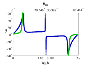
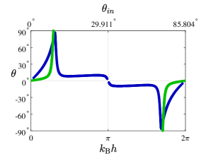
Figure 9: The transmitted angle $\theta$ of Bloch modes in laminate (23), induced by a pressure wave impinging at $x_{2}=0$ from the half-space (37), as function of incoming angle $\theta_{i}$ (upper axis) and its corresponding $k_{\mathrm{B}}h$ (lower axis). The frequency is $60\,$kHz in panel (a), and $60.1\,$kHz in panel (b). The colors identify corresponding branches of the same color in Fig. 5.

We proceed to analyze the transmission of Bloch modes in laminate (23) that are induced by impinging pressure wave from the half-space

$$\mu^{\left(0\right)}=0.033\,\mathrm{GPa},\ \lambda^{\left(0\right)}=0.132\,\mathrm{GPa},\ \rho^{\left(0\right)}=3000\,\mathrm{kg/m^{3}}.$$ (37)

To this end, we plot in Fig. 9 the propagation angle $\theta$ of the modes analyzed in Fig. 5, as functions of the incoming angle $\theta_{i}$ and its corresponding $k_{\mathrm{B}}h$, indicated by the upper and lower axes, respectively. The calculation of $\theta$ was carried out through direct evaluation of Eqs. (21)-(22) for calculate $\arctan\frac{\left\langle\mathcal{P}_{1}\right\rangle}{\left\langle\mathcal{P}_{2}\right\rangle}$.

Panel 9(a) is for $f=60\,$kHz, which corresponds to Fig. 5(a), and uses the same color legend. Our first observation concerns the change of sign in $\theta$ with respect to $k_{\mathrm{B}}h=\pi$, owing to the $2\pi$-periodicity of the spectrum in Re$\,k_{\mathrm{B}}h$, and its and reflection symmetry within that Brillouin zone period. Accordingly, $\partial\omega/\partial k_{\mathrm{B}}$ changes sign, and hence so does $\left\langle\mathcal{P}_{1}\right\rangle$, as noted by Willis (2015) in his analysis of anti-plane shear. The diagram exhibits 2-fold rotational symmetry about $\left(\pi,0\right)$, which corresponds to $\theta_{i}\approx 30^{\circ}$. Notably, the transmission angle of the blue mode increases very fast near $k_{\mathrm{B}}h=3.101$, and then discontinuously flips from $90^{\circ}$ to $-90^{\circ}$ at $k_{\mathrm{B}}h=3.182$. This discontinuity occurs since the blue branch does not exist (a gap) when $3.101<k_{\mathrm{B}}h<\pi$, as highlighted in Fig. 5(a). Therefore, in the vicinity $\theta_{i}\approx 30^{\circ}$, it is sufficient to slightly change the incident angle in order to significantly steer the transmitted mechanical beam. Wide steering by small changes of the incident angle, albeit less extreme, occurs also about $\theta_{i}\approx 10^{\circ}$ and $55^{\circ}$. We further note that since there is a range of $k_{\mathrm{B}}h$—and hence of incident angles—in which there is only one propagating mode (see Sec. 3), it is possible to achieve purely negative transmission. Analogous observations were made by Srivastava (2016) for anti-plane shear waves.

Panel 9(b) is for $f=60.1\,$kHz, which corresponds to Fig. 5(b). We observe that the discontinuous sign flip of $\theta$ and significant beam steering are lost, as the $\theta\left(k_{\mathrm{B}}h\right)$-curve smoothly passes through the point $\left(0,\pi\right)$. This result agrees with the extension of the blue branch in Fig. 5(b) to $\pi$ near $k_{2}h=0$, where it has an imaginary part, hence becomes attenuating. Thus, in the vicinity of $f=60\,\mathrm{kHz}$, energy transport is also very sensitive to the excitation frequency.

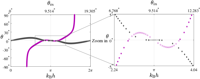
Figure 10: The transmitted angle $\theta$ of Bloch modes in laminate (23), induced by a pressure wave impinging at $x_{2}=0$ from the half-space (37), as function of incoming angle $\theta_{i}$ (upper axis) and its corresponding $k_{\mathrm{B}}h$ (lower axis), $f=181.3\,$kHz. Purple denotes the solutions with $k_{2}h<0.5$, where grey denotes solutions with $0.93<k_{2}h<1.21$. Segments above and below the exceptional points Fig. 5(e) are marked using circle marks and diamond marks, respectively.

Fig. 10 is for $f=181.3\,$kHz, corresponding to Fig. 5(e), which we recall exhibits two exceptional points; a zoom in about these points is shown in the right side of the figure. The color legend is different here: purple denotes solutions with $k_{2}h<0.5$, i.e., left to the first exceptional point in Fig. 5(e), where grey denotes solutions right to the second exceptional point, with $0.93<k_{2}h<1.21$. (Note that we do not include the third propagating branch with $3.4<k_{2}h$.) We mark the segments above and below the exceptional points Fig. 5(e) using circle marks and diamond marks, respectively.

Up to the first exceptional point $\left(k_{\mathrm{B}}h\approx 2.564,\theta_{i}\approx 7.753^{\circ}\right)$, the green branch of Fig. 5(e) admits two propagation angles which—remarkably—one of them is negative inside the first Brillouin zone. Beyond the exceptional point, mode switching occurs between the green branch (purple diamonds) and the blue branch (purple circles) of Fig. 5(e), as the former becomes attenuating and the latter becomes propagating with positive refraction. Similar switching occurs between the green and blue branches beyond the second exceptional point $\left(k_{\mathrm{B}}h\approx 3.021,\theta_{i}\approx 9.146^{\circ}\right)$. These phenomena are unique to the in-plane motion, owing to exceptional points, and are not accessible in the anti-plane setting. Finally, we note that here again, the diagram exhibits 2-fold rotational symmetry about $\left(\pi,0\right)$, which corresponds to $\theta_{i}\approx 9.514^{\circ}$, followed by the inversion of the aforementioned phenomena with respect to the incident angle.s

5 Conclusions

We have revisited the problem of in-plane waves propagation in periodic laminates, were the motivation was twofold. Firstly, this study is a necessary complement to the reports of Willis (2015), Nemat-Nasser (2015) and Srivastava (2016) on metamaterial phenomena in the model problem of anti-plane waves traversing elastic laminates. Secondly, this problem allows us to show that the coupling between shear and pressure parts can be harnessed for anomalous energy transport, within a relatively simple analytical study.

We have shown that the corresponding spectrum contains exceptional points at which two Bloch modes coalesce, and further showed that these points are the source of anomalous energy transport. To this end, we have determined how energy is scattered when an incident in-plane wave impinges the laminate in two model interface problems. We found metamaterial transmission through the laminate, such as pure negative refraction, and beam splitting and steering, at states of the system near the exceptional points. Notably, we achieved negative refraction in the canonical transmission problem, where the laminate is impinged by an incoming wave from a homogeneous medium whose interface with the laminate is parallel to the layers.

We emphasize again that these phenomena emerge from the unique coupling in elastodynamics between the volumetric and distortional modes of deformation, which cannot be observed in sound and light waves. Our work further paves the way for encircling exceptional points in a tangible, purely elastic apparatus, for applications such as asymmetric mode switches.

Appendix A

The forthcoming formulation is an adaptation of the developments of Shmuel and Pernas-Salomón (2016) and Pernas-Salomón and Shmuel (2018) to the current problem. Here, the modified state vector—consisting of quantities which are continuous across the interface between two adjacent layers—is

$$\mathsf{s_{m}}\left(x_{1},x_{2}\right)=\left(u_{1}\left(x_{1},x_{2}\right)C_{u_{1}},\ \sigma_{11}\left(x_{1},x_{2}\right)C_{\sigma_{11}},\ u_{2}\left(x_{1},x_{2}\right)C_{u_{2}},\ \sigma_{21}\left(x_{1},x_{2}\right)C_{\sigma_{21}}\right)^{\mathsf{T}},$$ (A.1)

where the normalizing coefficients required to stabilize subsequent calculations are

$$\begin{array}[]{ll}C_{u_{1}}=\left|k_{2}\right|^{-1},&C_{\sigma_{11}}=\left(\bar{\lambda}\left|k_{2}\right|\left|\bar{k_{L}}\right|\right)^{-1},\\ C_{u_{2}}=\left|k_{2}\right|^{-1},&C_{\sigma_{21}}=\left(\bar{\mu}\left|k_{2}\right|\left|\bar{k_{S}}\right|\right)^{-1},\end{array}$$ (A.2)

and

$$\begin{array}[]{l}\bar{k_{S}}=\left(k_{S}^{\left(\emph{a}\right)}+k_{S}^{\left(\emph{b}\right)}\right)/2,\\ \bar{k_{L}}=\left(k_{L}^{\left(\emph{a}\right)}+k_{L}^{\left(\emph{b}\right)}\right)/2,\\ \bar{\mu}=\left(\mu^{\left(\emph{a}\right)}+\mu^{\left(\emph{b}\right)}\right)/2,\\ \bar{\lambda}=\left[\left(\lambda^{\left(\emph{a}\right)}+\mu^{\left(\emph{a}\right)}+\lambda^{\left(\emph{b}\right)}+\mu^{\left(\emph{b}\right)}\right)/2+\bar{\mu}\right]/2.\end{array}$$ (A.3)

The state vector can be written as follows

$$\mathsf{s_{m}}\left(x_{1},x_{2}\right)=\mathsf{Q}\left(x_{1},x_{2}\right)\cdot\left(A_{L+}^{\left(n\right)},\ A_{S+}^{\left(\emph{n}\right)},\ A_{L-}^{\left(\emph{n}\right)},\ A_{S-}^{\left(\emph{n}\right)}\right)^{\mathsf{T}},$$ (A.4)

where

$$\begin{array}[]{l}\mathsf{Q}\left(x_{1},x_{2}\right)=\left(1/C_{u_{1}},\ 1/C_{\sigma_{11}},\ 1/C_{u_{2}},\ 1/C_{\sigma_{21}}\right)\cdot\\ \left(\begin{array}[]{llll}ik_{L}^{\left(\emph{p}\right)}&-ik_{2}&-ik_{L}^{\left(\emph{p}\right)}&-ik_{2}\\ -\lambda^{\left(\emph{p}\right)}k_{2}^{2}-\left(\lambda^{\left(\emph{p}\right)}+2\mu^{\left(\emph{p}\right)}\right)k_{L}^{2\left(\emph{p}\right)}&2\mu^{\left(\emph{p}\right)}k_{S}^{\left(\emph{p}\right)}k_{2}&-\lambda^{\left(\emph{p}\right)}k_{2}^{2}-\left(\lambda^{\left(\emph{p}\right)}+2\mu^{\left(\emph{p}\right)}\right)k_{L}^{2\left(\emph{p}\right)}&-2\mu^{\left(\emph{p}\right)}k_{S}^{\left(\emph{p}\right)}k_{2}\\ -ik_{2}&-ik_{S}^{\left(\emph{p}\right)}&-ik_{2}&ik_{S}^{\left(\emph{p}\right)}\\ 2\mu^{\left(\emph{p}\right)}k_{L}^{\left(\emph{p}\right)}k_{2}&\mu^{\left(\emph{p}\right)}\left(k_{S}^{2\left(\emph{p}\right)}-k_{2}^{2}\right)&-2\mu^{\left(\emph{p}\right)}k_{L}^{\left(\emph{p}\right)}k_{2}&\mu^{\left(\emph{p}\right)}\left(k_{S}^{2\left(\emph{p}\right)}-k_{2}^{2}\right)\end{array}\right)\\ \cdot\left(e^{ik_{L}^{\left(\emph{p}\right)}x1},\ e^{ik_{S}^{\left(\emph{p}\right)}x1},\ e^{-ik_{L}^{\left(\emph{p}\right)}x1},\ e^{-ik_{S}^{\left(\emph{p}\right)}x1}\right)e^{-ik_{2}x_{2}}.\end{array}$$ (A.5)

$\mathsf{Q}\left(x_{1},x_{2}\right)$ can also be defined as

$$\mathsf{Q}\left(x_{1},x_{2}\right) = \left(\begin{array}[]{llll}\mathsf{F}_{1}\left(x_{1},x_{2}\right)&\mathsf{F}_{2}\left(x_{1},x_{2}\right)&\mathsf{F}_{3}\left(x_{1},x_{2}\right)&\mathsf{F}_{4}\left(x_{1},x_{2}\right)\\ \mathsf{A}_{1}\left(x_{1},x_{2}\right)&\mathsf{A}_{2}\left(x_{1},x_{2}\right)&\mathsf{A}_{3}\left(x_{1},x_{2}\right)&\mathsf{A}_{4}\left(x_{1},x_{2}\right)\end{array}\right).$$ (A.8)

Using this definition the hybrid matrix of the $\emph{n}^{\mathrm{th}}$ layer is given by

$$\mathsf{H}^{\left(\emph{n}\right)}\left(h^{\left(\emph{p}\right)}\right)= \left(\begin{array}[]{llll}\mathsf{F}_{1}\left(x_{0},x_{2}\right)&\mathsf{F}_{2}\left(x_{0},x_{2}\right)&\mathsf{F}_{3}\left(x_{0},x_{2}\right)&\mathsf{F}_{4}\left(x_{0},x_{2}\right)\\ \mathsf{A}_{1}\left(x_{0}+h^{\left(\emph{p}\right)},x_{2}\right)&\mathsf{A}_{2}\left(x_{0}+h^{\left(\emph{p}\right)},x_{2}\right)&\mathsf{A}_{3}\left(x_{0}+h^{\left(\emph{p}\right)},x_{2}\right)&\mathsf{A}_{4}\left(x_{0}+h^{\left(\emph{p}\right)},x_{2}\right)\end{array}\right)$$ (A.9)

$$\left(\begin{array}[]{llll}\mathsf{A}_{1}\left(x_{0},x_{2}\right)&\mathsf{A}_{2}\left(x_{0},x_{2}\right)&\mathsf{A}_{3}\left(x_{0},x_{2}\right)&\mathsf{A}_{4}\left(x_{0},x_{2}\right)\\ \mathsf{F}_{1}\left(x_{0}+h^{\left(\emph{p}\right)},x_{2}\right)&\mathsf{F}_{2}\left(x_{0}+h^{\left(\emph{p}\right)},x_{2}\right)&\mathsf{F}_{3}\left(x_{0}+h^{\left(\emph{p}\right)},x_{2}\right)&\mathsf{F}_{4}\left(x_{0}+h^{\left(\emph{p}\right)},x_{2}\right)\end{array}\right)^{-1}.$$

Using the definition in Eq. (A.9), we relate the field variables which appear in the modified state vector at the ends $x_{0}$ and $x_{0}+h^{\left(\emph{p}\right)}$ of the $\emph{n}^{\mathrm{th}}$ layer via

$$\left(\begin{array}[]{l}u_{1}{}^{\left(n\right)}\left(x_{0},x_{2}\right)C_{u_{1}}\\ \sigma_{11}{}^{\left(n\right)}\left(x_{0},x_{2}\right)C_{\sigma_{11}}\\ u_{2}{}^{\left(n\right)}\left(x_{0}+h^{\left(\emph{p}\right)},x_{2}\right)C_{u_{2}}\\ \sigma_{21}{}^{\left(n\right)}\left(x_{0}+h^{\left(\emph{p}\right)},x_{2}\right)C_{\sigma_{21}}\end{array}\right)=\mathsf{H}^{\left(\emph{n}\right)}\left(h^{\left(\emph{p}\right)}\right)\cdot\left(\begin{array}[]{l}u_{2}{}^{\left(n\right)}\left(x_{0},x_{2}\right)C_{u_{2}}\\ \sigma_{21}{}^{\left(n\right)}\left(x_{0},x_{2}\right)C_{\sigma_{21}}\\ u_{1}{}^{\left(n\right)}\left(x_{0}+h^{\left(\emph{p}\right)},x_{2}\right)C_{u_{1}}\\ \sigma_{11}{}^{\left(n\right)}\left(x_{0}+h^{\left(\emph{p}\right)},x_{2}\right)C_{\sigma_{11}}\end{array}\right),$$ (A.10)

where $\mathsf{H}^{\left(\emph{n}\right)}\left(h^{\left(\emph{p}\right)}\right)$ is the $4\times 4$ hybrid matrix of the $\emph{n}^{\mathrm{th}}$ layer. In order to calculate the total hybrid matrix of n layers, denoted by $\mathsf{H}^{\left(1,n\right)}$, a recursive algorithm is used in terms of the hybrid matrix of the first $\emph{n}-1$ layers ($\mathsf{H}^{\left(1,n-1\right)}$) and the hybrid matrix of the $n^{\mathrm{th}}$ layer $\mathsf{H}^{\left(\emph{n}\right)}$, namely,

$$\mathsf{H}_{22}^{(1,k)} =\mathsf{H}_{22}^{\left(k\right)}+\mathsf{H}_{21}^{\left(k\right)}\cdot\left[\mathsf{I}_{2}-\mathsf{H}_{22}^{(1,k-1)}\cdot\mathsf{H}_{11}^{\left(k\right)}\right]^{-1}\cdot\mathsf{H}_{22}^{(1,k-1)}\cdot\mathsf{H}_{12}^{\left(k\right)},$$ (A.11)

$$\mathsf{H}_{21}^{(1,k)} =\mathsf{H}_{21}^{\left(k\right)}\cdot\left[\mathsf{I}_{2}-\mathsf{H}_{22}^{(1,k-1)}\cdot\mathsf{H}_{11}^{\left(k\right)}\right]^{-1}\cdot\mathsf{H}_{21}^{\left(1,k-1\right)},$$

$$\mathsf{H}_{12}^{(1,k)} =\mathsf{H}_{12}^{(1,k-1)}\cdot\mathsf{H}_{12}^{\left(k\right)}+\mathsf{H}_{12}^{(1,k-1)}\cdot\mathsf{H}_{11}^{\left(k\right)}\cdot\left[\mathsf{I}_{2}-\mathsf{H}_{22}^{(1,k-1)}\cdot\mathsf{H}_{11}^{\left(k\right)}\right]^{-1}\cdot\mathsf{H}_{22}^{(1,k-1)}\cdot\mathsf{H}_{12}^{\left(k\right)},$$

$$\mathsf{H}_{11}^{(1,k)} =\mathsf{H}_{11}^{(1,k-1)}+\mathsf{H}_{12}^{(1,k-1)}\cdot\mathsf{H}_{11}^{\left(k\right)}\cdot\left[\mathsf{I}_{2}-\mathsf{H}_{22}^{(1,k-1)}\cdot\mathsf{H}_{11}^{\left(k\right)}\right]^{-1}\cdot\mathsf{H}_{21}^{(1,k-1)},$$

Where $\mathsf{H}_{11}^{\left(1,k\right)},\mathsf{H}_{12}^{\left(1,k\right)},\mathsf{H}_{21}^{\left(1,k\right)},\mathsf{H}_{22}^{\left(1,k\right)}$ denote the $2\times 2$ blocks of the hybrid matrix $\mathsf{H}^{\left(1,k\right)}$ of the first $k$ layers. The generalized eigenproblem presented in Eq. (8) yields the characteristic equation

$$a_{1}+\lambda a_{2}+\lambda^{2}a_{3}+\lambda^{3}a_{4}+\lambda^{4}a_{5}=0$$ (A.12)

for $\lambda=e^{ik_{\mathrm{B}}h}$, where

$$a_{1}=h_{13}h_{24}-h_{14}h_{23}=\mathrm{det}\,\mathsf{H}_{12},$$ (A.13)

$$a_{2}=-h_{13}h_{42}h_{31}-h_{24}h_{42}h_{31}+h_{12}h_{43}h_{31}+h_{22}h_{44}h_{31}-h_{31}+h_{13}h_{32}h_{41}$$

$$+h_{24}h_{32}h_{41}-h_{12}h_{33}h_{41}-h_{22}h_{34}h_{41}$$

$$+h_{11}h_{33}h_{42}+h_{21}h_{34}h_{42}-h_{42}-h_{11}h_{32}h_{43}-h_{21}h_{32}h_{44},$$

$$a_{3}=1+h_{13}h_{31}+h_{24}h_{31}-h_{14}h_{23}h_{42}h_{31}+h_{13}h_{24}h_{42}h_{31}+h_{14}h_{22}h_{43}h_{31}$$

$$-h_{12}h_{24}h_{43}h_{31}-h_{13}h_{22}h_{44}h_{31}+h_{12}h_{23}h_{44}h_{31}-h_{11}h_{33}-h_{21}h_{34}$$

$$+h_{14}h_{23}h_{32}h_{41}-h_{13}h_{24}h_{32}h_{41}-h_{14}h_{22}h_{33}h_{41}+h_{12}h_{24}h_{33}h_{41}+h_{13}h_{22}h_{34}h_{41}$$

$$-h_{12}h_{23}h_{34}h_{41}+h_{13}h_{42}+h_{24}h_{42}+h_{14}h_{21}h_{33}h_{42}-h_{11}h_{24}h_{33}h_{42}$$

$$-h_{13}h_{21}h_{34}h_{42}+h_{11}h_{23}h_{34}h_{42}-h_{12}h_{43}-h_{14}h_{21}h_{32}h_{43}+h_{11}h_{24}h_{32}h_{43}$$

$$+h_{12}h_{21}h_{34}h_{43}-h_{11}h_{22}h_{34}h_{43}-h_{22}h_{44}+h_{13}h_{21}h_{32}h_{44}-h_{11}h_{23}h_{32}h_{44}$$

$$-h_{12}h_{21}h_{33}h_{44}+h_{11}h_{22}h_{33}h_{44},$$

$$a_{5}=a_{1},\ a_{4}=a_{2},$$

and $h_{ij}$ are the components of the total hybrid matrix. The latter two equalities imply that $\lambda^{-1}=e^{-ik_{\mathrm{B}}h}$ is also a solution, as expected. Eq. (A.12) yields a closed-form expression for $\cos k_{\mathrm{B}}h$, given in Eq. (9).

Appendix B

The matrices $\mathsf{A}_{0},\mathsf{A}_{1},\mathsf{A}_{2}$ and $\mathsf{B}$ appearing in Eq. (16) are given by

$$\begin{aligned} \mathsf{A}_{0}=\left(\begin{array}[]{ll}\mathsf{A}_{0}^{11}&\mathsf{0}\\ \mathsf{0}&\mathsf{A}_{0}^{22}\end{array}\right),\ \mathsf{A}_{1}=\left(\begin{array}[]{ll}\mathsf{0}&\mathsf{A}_{1}^{12}\\ \mathsf{A}_{1}^{21}&\mathsf{0}\end{array}\right),\ \mathsf{A}_{2}=\left(\begin{array}[]{ll}\mathsf{A}_{2}^{11}&\mathsf{0}\\ \mathsf{0}&\mathsf{A}_{2}^{22}\end{array}\right),\ \mathsf{B}=\left(\begin{array}[]{ll}\mathsf{B}^{11}&\mathsf{0}\\ \mathsf{0}&\mathsf{B}^{22}\end{array}\right)\end{aligned},$$ (B.1)

where the $\left(\mathrm{G},\mathrm{G^{\prime}}\right)$ component of each block is

$$\mathsf{A}_{0\ \mathrm{G}\mathrm{G^{\prime}}}^{11}=-\left[\left(\mathrm{G}+k_{\mathrm{B}}\right)\left(\mathrm{G^{\prime}}+k_{\mathrm{B}}\right)\right]\left[\lambda\left(\mathrm{G}-\mathrm{G^{\prime}}\right)+2\mu\left(\mathrm{G}-\mathrm{G^{\prime}}\right)\right],$$ (B.2)

$$\mathsf{A}_{0\ \mathrm{G}\mathrm{G^{\prime}}}^{22}=-\left[\left(\mathrm{G}+k_{\mathrm{B}}\right)\left(\mathrm{G^{\prime}}+k_{\mathrm{B}}\right)\right]\mu\left(\mathrm{G}-\mathrm{G^{\prime}}\right),$$

$$\mathsf{A}_{1\ \mathrm{G}\mathrm{G^{\prime}}}^{12}=\mathsf{A}_{1\ \mathrm{G},\mathrm{G^{\prime}}}^{21}=-\left(\mathrm{G}+k_{\mathrm{B}}\right)\left[\lambda\left(\mathrm{G}-\mathrm{G^{\prime}}\right)+\mu\left(\mathrm{G}-\mathrm{G^{\prime}}\right)\right],$$

$$\mathsf{A}_{2\ \mathrm{G}\mathrm{G^{\prime}}}^{11}=-\mu\left(\mathrm{G}-\mathrm{G^{\prime}}\right),$$

$$\mathsf{A}_{2\ \mathrm{G}\mathrm{G^{\prime}}}^{22}=-\lambda\left(\mathrm{G}-\mathrm{G^{\prime}}\right)-2\mu\left(\mathrm{G}-\mathrm{G^{\prime}}\right),$$

$$\mathsf{B}_{\mathrm{G}\mathrm{G^{\prime}}}^{11}=\mathsf{B}_{\mathrm{G},\mathrm{G^{\prime}}}^{22}=-\rho\left(\mathrm{G}-\mathrm{G^{\prime}}\right).$$

Appendix C

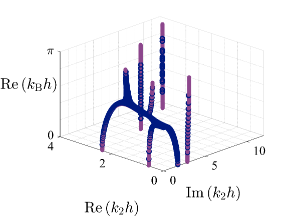
Figure 11: real $k_{\mathrm{B}}h$ as function of the real and imaginary parts of $k_{2}h$ for laminate (23) and $f=100\ \mathrm{kHz}$, using the EPWE and Hybrid matrix method, depicted in purple and blue points, respectively.

This appendix demonstrate the applicability of the extended plane wave expansion method, by comparing its results with the exact results of the hybrid matrix method. Fig. 11 shows real $k_{\mathrm{B}}h$ as function of the real and imaginary parts of $k_{2}h$ for laminate (23) and $f=100\ \mathrm{kHz}$. Points calculated with the extended plane wave expansion method and hybrid matrix method are depicted in purple and blue, respectively. We used 51 plane waves for the extended plane wave expansion method and points calculated using the hybrid matrix method differ from the results of the hybrid matrix by $5\times 10^{-2}$.

Appendix D

The components of the submatrices in Eq. 35 are

$$\mathsf{M}_{TT_{mm}}^{\mathsf{s}}=\frac{4ih}{\omega}\left\langle\mathcal{P}_{2}\right\rangle_{T}^{\left(m\right)},$$ (B.1)

$$\mathsf{M}_{T\phi_{ml}}^{\mathsf{s}}=\int_{0}^{h}\left[\mathsf{s}_{\phi_{1}}^{\perp}{}^{\left(l\right)}\mathsf{s}_{T_{3}}^{\perp}{}^{*}{}^{\left(m\right)}+\mathsf{s}_{\phi_{2}}^{\perp}{}^{\left(l\right)}\mathsf{s}_{T_{4}}^{\perp}{}^{*}{}^{\left(m\right)}-\left(\mathsf{s}_{\phi_{3}}^{\perp}{}^{\left(l\right)}\mathsf{s}_{T_{1}}^{\perp}{}^{*}{}^{\left(m\right)}+\mathsf{s}_{\phi_{4}}^{\perp}{}^{\left(l\right)}\mathsf{s}_{T_{2}}^{\perp}{}^{*}{}^{\left(m\right)}\right)\right]\mathrm{d}x_{1},$$

$$\mathsf{M}_{T\psi_{ml}}^{\mathsf{s}}=\int_{0}^{h}\left[\mathsf{s}_{\psi_{1}}^{\perp}{}^{\left(l\right)}\mathsf{s}_{T_{3}}^{\perp}{}^{*}{}^{\left(m\right)}+\mathsf{s}_{\psi_{2}}^{\perp}{}^{\left(l\right)}\mathsf{s}_{T_{4}}^{\perp}{}^{*}{}^{\left(m\right)}-\left(\mathsf{s}_{\psi_{3}}^{\perp}{}^{\left(l\right)}\mathsf{s}_{T_{1}}^{\perp}{}^{*}{}^{\left(m\right)}+\mathsf{s}_{\psi_{4}}^{\perp}{}^{\left(l\right)}\mathsf{s}_{T_{2}}^{\perp}{}^{*}{}^{\left(m\right)}\right)\right]\mathrm{d}x_{1},$$

$$\mathsf{M}_{\phi T_{lm}}^{\mathsf{s}}=\int_{0}^{h}\left[\mathsf{s}_{T_{1}}^{\perp}{}^{\left(m\right)}\mathsf{s}_{\phi_{3}}^{\perp}{}^{*}{}^{\left(l\right)}+\mathsf{s}_{T_{2}}^{\perp}{}^{\left(m\right)}\mathsf{s}_{\phi_{4}}^{\perp}{}^{*}{}^{\left(l\right)}-\left(\mathsf{s}_{T_{3}}^{\perp}{}^{\left(m\right)}\mathsf{s}_{\phi_{1}}^{\perp}{}^{*}{}^{\left(l\right)}+\mathsf{s}_{T_{4}}^{\perp}{}^{\left(m\right)}\mathsf{s}_{\phi_{2}}^{\perp}{}^{*}{}^{\left(l\right)}\right)\right]\mathrm{d}x_{1},$$

$$\mathsf{M}_{\phi\phi_{ll}}^{\mathsf{s}}=\frac{4ih}{\omega}\left\langle\mathcal{P}_{2}\right\rangle_{\phi}^{\left(l\right)},$$

$$\mathsf{M}_{\psi T_{lm}}^{\mathsf{s}}=\int_{0}^{h}\left[\mathsf{s}_{T_{1}}^{\perp}{}^{\left(m\right)}\mathsf{s}_{\psi_{3}}^{\perp}{}^{*}{}^{\left(l\right)}+\mathsf{s}_{T_{2}}^{\perp}{}^{\left(m\right)}\mathsf{s}_{\psi_{4}}^{\perp}{}^{*}{}^{\left(l\right)}-\left(\mathsf{s}_{T_{3}}^{\perp}{}^{\left(m\right)}\mathsf{s}_{\psi_{1}}^{\perp}{}^{*}{}^{\left(l\right)}+\mathsf{s}_{T_{4}}^{\perp}{}^{\left(m\right)}\mathsf{s}_{\psi_{2}}^{\perp}{}^{*}{}^{\left(l\right)}\right)\right]\mathrm{d}x_{1},$$

$$\mathsf{M}_{\psi\psi_{ll}}^{\mathsf{s}}=\frac{4ih}{\omega}\left\langle\mathcal{P}_{2}\right\rangle_{\psi}^{\left(l\right)},$$

$$\mathsf{I}_{T_{m}}^{\mathsf{s}}=\int_{0}^{h}\left[\mathsf{s}_{I_{1}}^{\perp}\mathsf{s}_{T_{3}}^{\perp}{}^{*}{}^{\left(m\right)}+\mathsf{s}_{I_{2}}^{\perp}\mathsf{s}_{T_{4}}^{\perp}{}^{*}{}^{\left(m\right)}-\left(\mathsf{s}_{I_{3}}^{\perp}\mathsf{s}_{T_{1}}^{\perp}{}^{*}{}^{\left(m\right)}+\mathsf{s}_{I_{4}}^{\perp}\mathsf{s}_{T_{2}}^{\perp}{}^{*}{}^{\left(m\right)}\right)\right]\mathrm{d}x_{1},$$

$$\mathsf{I}_{\phi_{l}}^{\mathsf{s}}=\int_{0}^{h}\left[\mathsf{s}_{I_{1}}^{\perp}\mathsf{s}_{\phi_{3}}^{\perp}{}^{*}{}^{\left(l\right)}+\mathsf{s}_{I_{2}}^{\perp}\mathsf{s}_{\phi_{4}}^{\perp}{}^{*}{}^{\left(l\right)}-\left(\mathsf{s}_{I_{3}}^{\perp}\mathsf{s}_{\phi_{1}}^{\perp}{}^{*}{}^{\left(l\right)}+\mathsf{s}_{I_{4}}^{\perp}\mathsf{s}_{\phi_{2}}^{\perp}{}^{*}{}^{\left(l\right)}\right)\right]\mathrm{d}x_{1},$$

$$\mathsf{I}_{\psi_{l}}^{\mathsf{s}}=\int_{0}^{h}\left[\mathsf{s}_{I_{1}}^{\perp}\mathsf{s}_{\psi_{3}}^{\perp}{}^{*}{}^{\left(l\right)}+\mathsf{s}_{I_{2}}^{\perp}\mathsf{s}_{\psi_{4}}^{\perp}{}^{*}{}^{\left(l\right)}-\left(\mathsf{s}_{I_{3}}^{\perp}\mathsf{s}_{\psi_{1}}^{\perp}{}^{*}{}^{\left(l\right)}+\mathsf{s}_{I_{4}}^{\perp}\mathsf{s}_{\psi_{2}}^{\perp}{}^{*}{}^{\left(l\right)}\right)\right]\mathrm{d}x_{1},$$

where subscript numbers denote the component of $\mathsf{s}^{\perp}$, and subscript letters denote the potential from which this component is derived.

Appendix E

[figure]style=plain,subcapbesideposition=top

[]  []  []  []

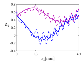
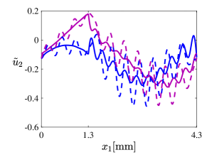
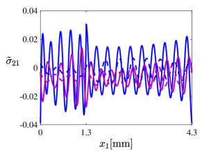
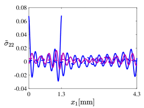
Figure 12: (a) $\mathsf{s}_{1}^{\perp}$ (b) $\mathsf{s}_{2}^{\perp}$ (c) $\mathsf{s}_{3}^{\perp}$ (d) $\mathsf{s}_{4}^{\perp}$ at the interface $x_{2}=0$ between laminate (23) and the homogeneous half-space (27), for $f=100\ \mathrm{kHz}$, $\theta_{i}=15.72^{\circ}$ an incident shear wave. The fields in the laminate (resp.  homogeneous half-space) fields are depicted in continuous (dashed) curves, where the real (imaginary) part is depicted in blue (purple).

Fig. 12 shows $\mathsf{s}_{1}^{\perp}$ (panel a), $\mathsf{s}_{2}^{\perp}$ (panel b), $\mathsf{s}_{3}^{\perp}$ (panel c, normalized by $k\bar{\mu}$), and $\mathsf{s}_{4}^{\perp}$ (panel d, normalized by $k\bar{\lambda}$) at the interface $x_{2}=0$ as calculated via Eq. (35). Specifically, solid and dashed curves correspond to the laminate and homogeneous half-space, respectively, where the real and imaginary parts of each field are denoted by blue and purple, respectively. The laminate and homogeneous half-space that was used have properties (23) and (27), respectively, and the calculation was carried out for $f=100\,\mathrm{kHz}$, $\theta_{i}=15.72^{\circ}$, and an incident shear wave. For this example, we chose $N_{R}=12$, which ensures all the propagating transmitted and reflected modes in the $x_{2}$ direction are included; the rest of the transmitted modes are those to have the lowest absolute value of $\mathrm{Im}k_{2}h$. The solution obtained does not match the fields perfectly, however it is sufficient on average provides a good approximation. The solution yields the following terms for the energy balance (36),

$$\begin{array}[]{ll}\left|T_{1}\right|^{2}\left\langle\mathcal{P}_{2}\right\rangle_{T}^{\left(1\right)}/\left|I\right|^{2}\left\langle\mathcal{P}_{2}\right\rangle_{I}=0.049,&\left|R_{-1}^{\psi}\right|^{2}\left\langle\mathcal{P}_{2}\right\rangle_{\psi}^{\left(-1\right)}/\left|I\right|^{2}\left\langle\mathcal{P}_{2}\right\rangle_{I}=-0.0133,\\ \left|R_{-1}^{\phi}\right|^{2}\text{$\left\langle\mathcal{P}_{2}\right\rangle_{\phi}^{\left(-1\right)}$}/\left|I\right|^{2}\left\langle\mathcal{P}_{2}\right\rangle_{I}=-0.091,&\left|R_{0}^{\psi}\right|^{2}\left\langle\mathcal{P}_{2}\right\rangle_{\psi}^{\left(0\right)}/\left|I\right|^{2}\left\langle\mathcal{P}_{2}\right\rangle_{I}=-0.437,\\ \left|R_{0}^{\phi}\right|^{2}\left\langle\mathcal{P}_{2}\right\rangle_{\phi}^{\left(0\right)}/\left|I\right|^{2}\left\langle\mathcal{P}_{2}\right\rangle_{I}=-0.391,&\left|R_{1}^{\psi}\right|^{2}\left\langle\mathcal{P}_{2}\right\rangle_{\psi}^{\left(1\right)}/\left|I\right|^{2}\left\langle\mathcal{P}_{2}\right\rangle_{I}=-0.007,\\ \left|R_{-2}^{\psi}\right|^{2}\left\langle\mathcal{P}_{2}\right\rangle_{\psi}^{\left(-2\right)}/\left|I\right|^{2}\left\langle\mathcal{P}_{2}\right\rangle_{I}=0,\end{array}$$ (B.1)

which sum to 0.988: a difference of only 0.12%. In this case, the transmitted mode refracts positively with transmitted angle of $\theta=1.12^{\circ}$, however carries only a small fraction of the energy of the incident wave.

References

- Achilleos et al. [2017] V. Achilleos, G. Theocharis, O. Richoux, and V. Pagneux. Non-hermitian acoustic metamaterials: Role of exceptional points in sound absorption. Phys. Rev. B, 95:144303, Apr 2017. doi: 10.1103/PhysRevB.95.144303. URL https://link.aps.org/doi/10.1103/PhysRevB.95.144303.
- Adams et al. [2008] S D M Adams, R V Craster, and S Guenneau. Bloch waves in periodic multi-layered acoustic waveguides. Proc. R. Soc. London A, 464(2098):2669–2692, 2008.
- Adams et al. [2009] Samuel D.M. Adams, Richard V. Craster, and Sebastien Guenneau. Guided and standing bloch waves in periodic elastic strips. Waves in Random and Complex Media, 19(2):321–346, 2009. doi: 10.1080/17455030802541566. URL https://doi.org/10.1080/17455030802541566.
- Aghighi et al. [2019] Fateme Aghighi, Joshua Morris, and Alireza V. Amirkhizi. Low-frequency micro-structured mechanical metamaterials. Mechanics of Materials, 130:65 – 75, 2019. ISSN 0167-6636. doi: https://doi.org/10.1016/j.mechmat.2018.12.008. URL http://www.sciencedirect.com/science/article/pii/S0167663618306483.
- Banerjee [2011] Biswajit Banerjee. An introduction to metamaterials and waves in composites. CRC Press, 2011.
- Bigoni et al. [2013] D Bigoni, S Guenneau, A B Movchan, and M Brun. Elastic metamaterials with inertial locally resonant structures: Application to lensing and localization. Phys. Rev. B, 87(17):174303, 2013. doi: 10.1103/PhysRevB.87.174303. URL https://link.aps.org/doi/10.1103/PhysRevB.87.174303.
- Bordiga et al. [2019] G. Bordiga, L. Cabras, A. Piccolroaz, and D. Bigoni. Prestress tuning of negative refraction and wave channeling from flexural sources. Applied Physics Letters, 114(4):041901, 2019. doi: 10.1063/1.5084258. URL https://doi.org/10.1063/1.5084258.
- Brun et al. [2010] M Brun, S Guenneau, A B Movchan, and D Bigoni. Dynamics of structural interfaces: Filtering and focussing effects for elastic waves. J. Mech. Phys. Solids, 58(9):1212–1224, 2010.
- Chen et al. [2010] Huanyang Chen, C. T. Chan, and Ping Sheng. Transformation optics and metamaterials. Nature Materials, 9:387 EP –, 04 2010. URL https://doi.org/10.1038/nmat2743.
- Chen and Elbanna [2017] Qianli Chen and Ahmed Elbanna. Emergent wave phenomena in coupled elastic bars: from extreme attenuation to realization of elastodynamic switches. Scientific Reports, 7(1):16204, 2017. doi: 10.1038/s41598-017-16364-8. URL https://doi.org/10.1038/s41598-017-16364-8.
- Chen et al. [2017] Y Chen, G Hu, and G Huang. A hybrid elastic metamaterial with negative mass density and tunable bending stiffness. J. Mech. Phys. Solids, 105:179–198, 2017. ISSN 0022-5096. doi: https://doi.org/10.1016/j.jmps.2017.05.009. URL http://www.sciencedirect.com/science/article/pii/S0022509617301229.
- Christensen et al. [2016] J Christensen, M Willatzen, V R Velasco, and M.-H. Lu. Parity-Time Synthetic Phononic Media. Phys. Rev. Lett., 116(20):207601, 2016. doi: 10.1103/PhysRevLett.116.207601. URL https://link.aps.org/doi/10.1103/PhysRevLett.116.207601.
- Colquitt et al. [2014] D J Colquitt, M Brun, M Gei, A B Movchan, N V Movchan, and I S Jones. Transformation elastodynamics and cloaking for flexural waves. J. Mech. Phys. Solids, 72:131–143, 2014. ISSN 0022-5096. doi: http://dx.doi.org/10.1016/j.jmps.2014.07.014. URL http://www.sciencedirect.com/science/article/pii/S0022509614001586.
- Craster and Guenneau [2012] Richard V Craster and Sébastien Guenneau. Acoustic metamaterials: Negative refraction, imaging, lensing and cloaking, volume 166. Springer Science & Business Media, 2012.
- Cummer et al. [2016] Steven A. Cummer, Johan Christensen, and Andrea Alù. Controlling sound with acoustic metamaterials. Nature Reviews Materials, 1:16001 EP –, 02 2016. URL https://doi.org/10.1038/natrevmats.2016.1.
- Deymier [2013] Pierre A Deymier. Acoustic metamaterials and phononic crystals, volume 173. Springer Science & Business Media, 2013.
- Ding et al. [2015] Kun Ding, Z Q Zhang, and C T Chan. Coalescence of exceptional points and phase diagrams for one-dimensional PT-symmetric photonic crystals. Phys. Rev. B, 92(23):235310, 2015. doi: 10.1103/PhysRevB.92.235310. URL https://link.aps.org/doi/10.1103/PhysRevB.92.235310.
- Doppler et al. [2016] Jörg Doppler, Alexei A Mailybaev, Julian Böhm, Ulrich Kuhl, Adrian Girschik, Florian Libisch, Thomas J Milburn, Peter Rabl, Nimrod Moiseyev, and Stefan Rotter. Dynamically encircling an exceptional point for asymmetric mode switching. Nature, 537:76 EP –, 2016. URL https://doi.org/10.1038/nature18605.
- El-Ganainy et al. [2018] Ramy El-Ganainy, Konstantinos G Makris, Mercedeh Khajavikhan, Ziad H Musslimani, Stefan Rotter, and Demetrios N Christodoulides. Non-Hermitian physics and PT symmetry. Nature Physics, 14:11 EP –, 2018. URL https://doi.org/10.1038/nphys4323.
- Goldzak et al. [2018] Tamar Goldzak, Alexei A Mailybaev, and Nimrod Moiseyev. Light Stops at Exceptional Points. Phys. Rev. Lett., 120(1):13901, 2018. doi: 10.1103/PhysRevLett.120.013901. URL https://link.aps.org/doi/10.1103/PhysRevLett.120.013901.
- Graff [1975] K F Graff. Wave Motion in Elastic Solids. Dover Books on Physics Series. Dover Publications, 1975. ISBN 9780486667454. URL https://books.google.co.il/books?id=5cZFRwLuhdQC.
- Hodaei et al. [2017] Hossein Hodaei, Absar U Hassan, Steffen Wittek, Hipolito Garcia-Gracia, Ramy El-Ganainy, Demetrios N Christodoulides, and Mercedeh Khajavikhan. Enhanced sensitivity at higher-order exceptional points. Nature, 548(7666):187, 2017.
- Hou and Assouar [2018] Zhilin Hou and Badreddine Assouar. Tunable elastic parity-time symmetric structure based on the shunted piezoelectric materials. Journal of Applied Physics, 123(8):85101, 2018. doi: 10.1063/1.5009129. URL https://doi.org/10.1063/1.5009129.
- Hou et al. [2018] Zhilin Hou, Huiqin Ni, and Badreddine Assouar. Pt-symmetry for elastic negative refraction. Phys. Rev. Applied, 10(4):44071, 2018. doi: 10.1103/PhysRevApplied.10.044071. URL https://link.aps.org/doi/10.1103/PhysRevApplied.10.044071.
- Hsue et al. [2005] Young-Chung Hsue, Arthur J. Freeman, and Ben-Yuan Gu. Extended plane-wave expansion method in three-dimensional anisotropic photonic crystals. Phys. Rev. B, 72:195118, Nov 2005. doi: 10.1103/PhysRevB.72.195118. URL https://link.aps.org/doi/10.1103/PhysRevB.72.195118.
- Hussein et al. [2014] M I Hussein, M J Leamy, and M Ruzzene. Dynamics of Phononic Materials and Structures: Historical Origins, Recent Progress, and Future Outlook. Appl. Mech. Rev., 66(4):40802, 2014. URL http://dx.doi.org/10.1115/1.4026911.
- Joseph and Craster [2015] L M Joseph and R V Craster. Reflection from a semi-infinite stack of layers using homogenization. Wave Motion, 54:145–156, 2015. ISSN 0165-2125. doi: https://doi.org/10.1016/j.wavemoti.2014.12.003. URL http://www.sciencedirect.com/science/article/pii/S0165212514001747.
- Kadic et al. [2019] Muamer Kadic, Graeme W. Milton, Martin van Hecke, and Martin Wegener. 3d metamaterials. Nature Reviews Physics, 1(3):198–210, 2019. doi: 10.1038/s42254-018-0018-y. URL https://doi.org/10.1038/s42254-018-0018-y.
- Kushwaha et al. [1993] M S Kushwaha, P Halevi, L Dobrzynski, and B Djafari-Rouhani. Acoustic band structure of periodic elastic composites. Phys. Rev. Lett., 71(13):2022–2025, 1993.
- Laude et al. [2009] Vincent Laude, Younes Achaoui, Sarah Benchabane, and Abdelkrim Khelif. Evanescent bloch waves and the complex band structure of phononic crystals. Phys. Rev. B, 80:092301, Sep 2009. doi: 10.1103/PhysRevB.80.092301. URL https://link.aps.org/doi/10.1103/PhysRevB.80.092301.
- Li and Reina [2019] Xiaoguai Li and Celia Reina. Simultaneous spatial and temporal coarse-graining: From atomistic models to continuum elastodynamics. Journal of the Mechanics and Physics of Solids, 130:118 – 140, 2019. ISSN 0022-5096. doi: https://doi.org/10.1016/j.jmps.2019.05.004. URL http://www.sciencedirect.com/science/article/pii/S0022509618310792.
- Lowe [1995] M J S Lowe. Matrix techniques for modeling ultrasonic waves in multilayered media. IEEE Trans. Ultrason. Ferroelectr. Freq. Control, 42(4):525–542, 1995. ISSN 0885-3010. doi: 10.1109/58.393096.
- Lu and Srivastava [2018] Yan Lu and Ankit Srivastava. Level repulsion and band sorting in phononic crystals. Journal of the Mechanics and Physics of Solids, 111:100–112, 2018.
- Ma et al. [2018] Jihong Ma, Di Zhou, Kai Sun, Xiaoming Mao, and Stefano Gonella. Edge modes and asymmetric wave transport in topological lattices: Experimental characterization at finite frequencies. Phys. Rev. Lett., 121:094301, Aug 2018. doi: 10.1103/PhysRevLett.121.094301. URL https://link.aps.org/doi/10.1103/PhysRevLett.121.094301.
- Markos and Soukoulis [2008] P Markos and C M Soukoulis. Wave Propagation. From Electrons to Photonic Crystals and Left-Handed Materials. New York, Wiley, 2008.
- Merkel et al. [2018] Aurélien Merkel, Vicent Romero-García, Jean-Philippe Groby, Jensen Li, and Johan Christensen. Unidirectional zero sonic reflection in passive -symmetric willis media. Phys. Rev. B, 98:201102, Nov 2018. doi: 10.1103/PhysRevB.98.201102. URL https://link.aps.org/doi/10.1103/PhysRevB.98.201102.
- Milton et al. [2006] G W Milton, M Briane, and J R Willis. On cloaking for elasticity and physical equations with a transformation invariant form. New J. Phys., 8(10):248, 2006. URL http://stacks.iop.org/1367-2630/8/i=10/a=248.
- Milton and Mattei [2017] Graeme W Milton and Ornella Mattei. Field patterns: a new mathematical object. Proc. R. Soc. London A Math. Phys. Eng. Sci., 473(2198), 2017. ISSN 1364-5021. doi: 10.1098/rspa.2016.0819. URL http://rspa.royalsocietypublishing.org/content/473/2198/20160819.
- Moiseyev [2011] Nimrod Moiseyev. Non-Hermitian Quantum Mechanics. Cambridge University Press, 2011. doi: 10.1017/CBO9780511976186.
- Moiseyev and Friedland [1980] Nimrod Moiseyev and Shmuel Friedland. Association of resonance states with the incomplete spectrum of finite complex-scaled Hamiltonian matrices. Phys. Rev. A, 22(2):618–624, 1980. doi: 10.1103/PhysRevA.22.618. URL https://link.aps.org/doi/10.1103/PhysRevA.22.618.
- Mokhtari et al. [2019] Amir Ashkan Mokhtari, Yan Lu, and Ankit Srivastava. On the properties of phononic eigenvalue problems. Journal of the Mechanics and Physics of Solids, 2019. ISSN 0022-5096. doi: https://doi.org/10.1016/j.jmps.2019.07.005. URL http://www.sciencedirect.com/science/article/pii/S0022509619304247.
- Morini et al. [2019] Lorenzo Morini, Yoann Eyzat, and Massimiliano Gei. Negative refraction in quasicrystalline multilayered metamaterials. Journal of the Mechanics and Physics of Solids, 124:282 – 298, 2019. ISSN 0022-5096. doi: https://doi.org/10.1016/j.jmps.2018.10.016. URL http://www.sciencedirect.com/science/article/pii/S0022509618306410.
- Nassar et al. [2017] H Nassar, X C Xu, A N Norris, and G L Huang. Modulated phononic crystals: Non-reciprocal wave propagation and Willis materials. Journal of the Mechanics and Physics of Solids, 101:10–29, 2017. ISSN 0022-5096. doi: https://doi.org/10.1016/j.jmps.2017.01.010. URL http://www.sciencedirect.com/science/article/pii/S0022509616308997.
- Nemat-Nasser [2015] Sia Nemat-Nasser. Anti-plane shear waves in periodic elastic composites: band structure and anomalous wave refraction. Proc. R. Soc. London A Math. Phys. Eng. Sci., 471(2180), 2015. ISSN 1364-5021. doi: 10.1098/rspa.2015.0152. URL http://rspa.royalsocietypublishing.org/content/471/2180/20150152.
- Nemat-Nasser [2019] Sia Nemat-Nasser. Inherent negative refraction on acoustic branch of two dimensional phononic crystals. Mechanics of Materials, 132:1 – 8, 2019. ISSN 0167-6636. doi: https://doi.org/10.1016/j.mechmat.2018.12.011. URL http://www.sciencedirect.com/science/article/pii/S016766361830752X.
- Parnell and Shearer [2013] William J. Parnell and Tom Shearer. Antiplane elastic wave cloaking using metamaterials, homogenization and hyperelasticity. Wave Motion, 50(7):1140 – 1152, 2013. ISSN 0165-2125. doi: https://doi.org/10.1016/j.wavemoti.2013.06.006. URL http://www.sciencedirect.com/science/article/pii/S0165212513001157. Advanced Modelling of Wave Propagation in Solids.
- Pendry [2004] J. B. Pendry. A chiral route to negative refraction. Science, 306(5700):1353–1355, 2004. ISSN 0036-8075. doi: 10.1126/science.1104467. URL https://science.sciencemag.org/content/306/5700/1353.
- Pérez-Álvarez et al. [2015] R Pérez-Álvarez, René Pernas-Salomón, and VR Velasco. Relations between transfer matrices and numerical stability analysis to avoid the problem. SIAM Journal on Applied Mathematics, 75(4):1403–1423, 2015.
- Pernas-Salomón and Shmuel [2018] René Pernas-Salomón and Gal Shmuel. Dynamic homogenization of composite and locally resonant flexural systems. J. Mech. Phys. Solids, 119:43–59, 2018. ISSN 0022-5096. doi: https://doi.org/10.1016/j.jmps.2018.06.011. URL http://www.sciencedirect.com/science/article/pii/S0022509618302503.
- Phani and Hussein [2017] A. S. Phani and M. I. Hussein, editors. Dynamics of lattice materials. Wiley, New York, 2017.
- Phani [2011] A Srikantha Phani. On elastic waves and related phenomena in lattice materials and structures. AIP Advances, 1(4):41602, 2011. doi: 10.1063/1.3676167. URL https://doi.org/10.1063/1.3676167.
- Raney et al. [2016] J Raney, N Nadkarni, C Daraio, D M Kochmann, J A Lewis, and K Bertoldi. Stable propagation of mechanical signals in soft media using stored elastic energy. Proc. Natl. Acad. Sci. U. S. A., 2016.
- Rüter et al. [2010] Christian E Rüter, Konstantinos G Makris, Ramy El-Ganainy, Demetrios N Christodoulides, Mordechai Segev, and Detlef Kip. Observation of parity–time symmetry in optics. Nature physics, 6(3):192, 2010.
- Shanin et al. [2018] A.V. Shanin, K.S. Knyazeva, and A.I. Korolkov. Riemann surface of dispersion diagram of a multilayer acoustical waveguide. Wave Motion, 83:148 – 172, 2018. ISSN 0165-2125. doi: https://doi.org/10.1016/j.wavemoti.2018.09.010. URL http://www.sciencedirect.com/science/article/pii/S0165212518303871.
- Shelby et al. [2001] Richard A Shelby, David R Smith, and Seldon Schultz. Experimental verification of a negative index of refraction. science, 292(5514):77–79, 2001.
- Shi et al. [2016] Chengzhi Shi, Marc Dubois, Yun Chen, Lei Cheng, Hamidreza Ramezani, Yuan Wang, and Xiang Zhang. Accessing the exceptional points of parity-time symmetric acoustics. Nature communications, 7:11110, 2016.
- Shmuel and Band [2016] G Shmuel and R Band. Universality of the frequency spectrum of laminates. J. Mech. Phys. Solids, 92:127–136, 2016. ISSN 0022-5096. doi: http://dx.doi.org/10.1016/j.jmps.2016.04.001.
- Shmuel and Pernas-Salomón [2016] G Shmuel and R Pernas-Salomón. Manipulating motions of elastomer films by electrostatically-controlled aperiodicity. Smart Mater. Struct., 25(12):125012, 2016. ISSN 1361665X. doi: 10.1088/0964-1726/25/12/125012. URL http://stacks.iop.org/0964-1726/25/i=12/a=125012.
- Sigalas and Economou [1992] M M Sigalas and E N Economou. Elastic and acoustic wave band structure. J. Sound Vib., 158(2):377–382, 1992.
- Smith et al. [2000] D. R. Smith, Willie J. Padilla, D. C. Vier, S. C. Nemat-Nasser, and S. Schultz. Composite medium with simultaneously negative permeability and permittivity. Phys. Rev. Lett., 84:4184–4187, May 2000. doi: 10.1103/PhysRevLett.84.4184. URL https://link.aps.org/doi/10.1103/PhysRevLett.84.4184.
- Srivastava [2016] A Srivastava. Metamaterial properties of periodic laminates. J. Mech. Phys. Solids, 96:252–263, 2016. ISSN 0022-5096. doi: http://dx.doi.org/10.1016/j.jmps.2016.07.018. URL http://www.sciencedirect.com/science/article/pii/S0022509616303933.
- Srivastava and Willis [2017] A Srivastava and J R Willis. Evanescent wave boundary layers in metamaterials and sidestepping them through a variational approach. Proc. R. Soc. London A Math. Phys. Eng. Sci., 473(2200), 2017. ISSN 1364-5021. doi: 10.1098/rspa.2016.0765. URL http://rspa.royalsocietypublishing.org/content/473/2200/20160765.
- Tan [2010] E L Tan. Generalized eigenproblem of hybrid matrix for Floquet wave propagation in one-dimensional phononic crystals with solids and fluids. Ultrasonics, 50(1):91–98, 2010. ISSN 0041-624X. doi: http://dx.doi.org/10.1016/j.ultras.2009.09.007. URL http://www.sciencedirect.com/science/article/pii/S0041624X09001085.
- Torrent and Sánchez-Dehesa [2011] Daniel Torrent and José Sánchez-Dehesa. Multiple scattering formulation of two-dimensional acoustic and electromagnetic metamaterials. New Journal of Physics, 13(9):093018, sep 2011. doi: 10.1088/1367-2630/13/9/093018. URL https://doi.org/10.1088%2F1367-2630%2F13%2F9%2F093018.
- Torrent et al. [2018] Daniel Torrent, William J. Parnell, and Andrew N. Norris. Loss compensation in time-dependent elastic metamaterials. Phys. Rev. B, 97:014105, Jan 2018. doi: 10.1103/PhysRevB.97.014105. URL https://link.aps.org/doi/10.1103/PhysRevB.97.014105.
- Trainiti and Ruzzene [2016] G Trainiti and M Ruzzene. Non-reciprocal elastic wave propagation in spatiotemporal periodic structures. New Journal of Physics, 18(8):083047, aug 2016. doi: 10.1088/1367-2630/18/8/083047. URL https://doi.org/10.1088%2F1367-2630%2F18%2F8%2F083047.
- Wegener [2013] Martin Wegener. Metamaterials beyond optics. Science, 342(6161):939–940, 2013. ISSN 0036-8075. doi: 10.1126/science.1246545. URL https://science.sciencemag.org/content/342/6161/939.
- Willis [2015] J R Willis. Negative refraction in a laminate. J. Mech. Phys. Solids, 97:10–18, 2015. ISSN 0022-5096. doi: http://dx.doi.org/10.1016/j.jmps.2015.11.004. URL http://www.sciencedirect.com/science/article/pii/S0022509615302623.
- Willis [2013] John Willis. A study of obliquely propagating longitudinal shear waves in a periodic laminate. arXiv e-prints, art. arXiv:1310.6561, Oct 2013.
- Xu et al. [2015] Xun-Wei Xu, Yu-xi Liu, Chang-Pu Sun, and Yong Li. Mechanical symmetry in coupled optomechanical systems. Phys. Rev. A, 92:013852, Jul 2015. doi: 10.1103/PhysRevA.92.013852. URL https://link.aps.org/doi/10.1103/PhysRevA.92.013852.
- Zelhofer and Kochmann [2017] A J Zelhofer and D M Kochmann. On acoustic wave beaming in two-dimensional structural lattices. Int. J. Solids Struct., 115-116:248–269, 2017. ISSN 0020-7683. doi: http://doi.org/10.1016/j.ijsolstr.2017.03.024. URL http://www.sciencedirect.com/science/article/pii/S0020768317301336.
- Zhang [2019] Pu Zhang. Symmetry and degeneracy of phonon modes for periodic structures with glide symmetry. Journal of the Mechanics and Physics of Solids, 122:244 – 261, 2019. ISSN 0022-5096. doi: https://doi.org/10.1016/j.jmps.2018.09.016. URL http://www.sciencedirect.com/science/article/pii/S0022509618304605.