NN-sort: Neural Network based Data Distribution-aware Sorting

Abstract.

Sorting is a fundamental operation in computing. However, the speed of state-of-the-art sorting algorithms on a single thread have reached their limits. Meanwhile, deep learning has demonstrated its potential to provide significant performance improvements on data mining and machine learning tasks. Therefore, it is interesting to explore whether sorting can also be speed up by deep learning techniques. In this paper, a neural network based data distribution aware sorting method named NN-sort is presented. Compared to traditional comparison-based sorting algorithms, which need to compare the data elements in pairwise, NN-sort leverages the neural network model to learn the data distribution and uses it to map disordered data elements into ordered ones. Although the complexity of NN-sort is $nlogn$ in theory, it can run in near-linear time as being observed in most of the cases. Experimental results on both synthetic and real-world datasets show that NN-sort yields performance improvement by up to $10.9$x over traditional sorting algorithms.

1. Introduction

Sorting is one of the most fundamental computational building blocks and has been commonly used in many applications where data needs to be organized in order, such as database systems (Graefe, 2006), recommendation systems (DBLP:journals/jiis/TerrientesVZB16a), bioinformatics (Hilker et al., 2012), and social networks (Li et al., 2019). With the development of distributed systems, sorting has also been widely adopted in cloud and big data environments. Taking the MapReduce jobs(Dean and Ghemawat, 2008) as an example, the intermediate key-value pairs produced by the map tasks need to be sorted by the keys before being shuffled to the reduce tasks, thus the effectiveness of sorting can largely affect the overall performance of such jobs.

In general, existing sorting methods can be categorized into two classes: comparison-based and non-comparison based. Examples of comparison-based sorting include Quick Sort (Cormen, [n. d.]), Tim Sort (peters2002python), and Merge Sort (Buss and Knop, 2019). In these approaches, the input data elements are rearranged by comparing their values. For non-comparison based sorting, such as Radix Sort (Andersson et al., 1998) , Counting Sort (de Gouw et al., 2014), and many others (Han, 2002; Han and Thorup, 2002; Kirkpatrick and Reisch, 1983; thorup2002randomized), instead of rearranging data elements by comparing their values, they perform sorting by taking the advantages of the internal characters of the items to be sorted. Compared with comparison-based sorting, which can sort in $O(nlogn)$ time, complexity of a non-comparison based sorting method can be reduced to $O(n)$.

In addition, hardware-specific sorting solutions have also been proposed, such as GPU-based Merge Sort (GPU-comparison-based-sort) and GPU-based Radix Sort (GPU-radix2). These algorithms aim to take the advantages of GPU hardware to parallel the tradition sorting algorithms for better sorting performance. However, as pointed in (Cook and Shane, [n. d.]), numerous traditional sorting algorithms failed to gain performance speed-up by using GPU to date. Some of the examples are Quick Sort and Heap Sort, which heavily rely on recursions, in which the intermediate results of the calculation highly interdependent. In this paper, we focus on accelerating the speed of single thread sorting.

Inspired by the recent success of deep neural networks in many data mining and machine learning tasks, we argue that one way to further scale the sorting to a large amount of data with high performance is to fundamentally change the existing sorting principle. Instead of iterating over the input data elements, we can train a neural network model based on historical data and then use this model to sort the new coming data. This approach is practical and promising due to a number of facts. First, large amount of data has been continuously collected through various channels such as IoT devices and monitoring systems, which makes it possible to train a well-performing and data distribution aware neural network model. Second, it is observed that data collected by a specific organization usually follows a consistent distribution. For example, as shown in (Jiang and Jia, 2011; Brockmann et al., 2006; radicchi2009human), data generated by a similar set of users are mostly subject to a certain stable empirical distribution. Although, as we will demonstrate later, NN-sort works well even if the sorting data has a different distribution than the sorting data, such observed data distribution consistency actually allows the NN-sort to achieve higher efficiency.

There are recent researches that investigate how deep learning models can be used to improve the performance of traditional systems and algorithms (Kraska et al., 2018, 2019; DBLP:journals/access/XiangZCCLZ19). Wenkun Xiang et al. (DBLP:journals/access/XiangZCCLZ19) showed a shorter average searching time by using a learned index structure to replace the traditional inverted index structure. Tim Kraska et al. (Kraska et al., 2019) introduced a learned hash-model index by learning an empirical cumulative distribution function at a reasonable cost. They briefly mentioned SageDB Sort (Kraska et al., 2019) which uses a cumulative distribution function model improve the sorting performance. However, it is still not clear how to design an effective deep learning base sorting algorithm. Specifically, what kind of neural network performs best for sorting, what are the opportunities and challenges in applying neural networks to sorting, how to balance between the model accuracy and sorting performance?

To the best of our knowledge, this paper is the first one to provide in-depth and systematic studies for the above-mentioned questions. In this paper, we present a neural network based sorting algorithm, named NN-sort. The key idea of NN-sort is to train a neural network model over the historical data and use it to sort the future data. Considering the fact that it is almost impossible to train an idea neural network model that never make mistakes, data needs to be polished after it is fed to the model, so as the guarantee the correctness of sorting. NN-sort is designed in a three-phase architecture: the input phase, the sorting phase, and the polish phase. The goal of the first phase is to pre-process the input dataset such as converting each input data elements to a vector so that they can be consumed by a neural network model. In the second phase, a deep neural network based model is trained, which maps an input vector to a value that reflects the position of the corresponding data element in the final sorted array. A conflicting array is used to resolve the conflicts when different input data elements are mapped to the same position. The model will run for multiple iterations in the sorting phase until the size of the conflicting array is smaller than a threshold, or the number of iterations reaches a pre-defined value. Two arrays are generated at the end of each iteration: a roughly sorted array and a conflicting array. Then, the conflicting array will be used as the input of the next iteration. In the polish phase, the last conflict array will be sorted using the traditional sorting approach, such as Quick Sort, and then be merged with the other roughly sorted array generated in the previous iterations to produce the final result. As the model could map some data elements out of order, a correct method is integrated into the polish phase to guarantee final output is strictly sorted.

Furthermore, complexity of NN-sort is analyzed by using a cost model to illustrate the relationship between the model accuracy and sorting performance. Experiments using both synthetic and real-world datasets with different empirical distributions are also carried out to compare the performance between NN-sort and other popular traditional sorting algorithms. The contributions of this paper are summarized as follows:

• We investigate and explore the opportunities and challenges to improve the traditional sorting problem by leveraging neural network based learning approaches.

• We develop NN-sort, a novel neural network based sorting approach. This approach takes the advantage of historical data to train a neural network model, which is data distribution aware. The trained model is capable of performing high-performance sorting on new coming data in an iterative way with additional touch-up to guarantee the correctness.

• We provide a formal analysis of the complexity of NN-sort using a cost model that illustrates the intrinsic relationship between model accuracy and sorting performance.

• We evaluate the performance of NN-sort by using both synthetic and real-world datasets. Experimental results show that NN-sort provides up to an order of magnitude speed-up in sorting time compared to the state-of-the-art sorting algorithms.

The rest of the paper is organized as follows: the related work and some background are introduced in Section 2. The NN-sort approach is presented in Section 3. The time complicity and the cost model are discussed in Section 4. The experimental evaluation results are reported in Section 5. we conclude the paper in Section 6.

2. Related Work

Sorting is one of the most widely studied algorithms. We identify three most relevant research threads in the sorting area: improving parallelism for high-performance sorting, methods for reducing the sorting time complexity, and neural network-based data structures.

Improving parallelism for high-performance sorting. There are orthogonal efforts on improving the parallelism of the algorithms to achieve high-performance sorting. For example, the implementation of the sorting algorithm on Hadoop distributed clusters is introduced in (Faghri et al., 2012). Wei Song et al. (DBLP:conf/fccm/SongKLG16) introduced a parallel hardware Merge Sort, which reduces the total sorting time by 160 times compared with traditional sequential sorting by using FPGAs. Bandyopadhyay and Sahni (Bandyopadhyay and Sahni, 2010) proposed to partition the data sequence to be sorted into sub-sequences, then sort these sub-sequences and merge the sorted sub-sequences in parallel. Baraglia et al. (Bandyopadhyay and Sahni, 2010) investigated optimal block-kernel mappings of a bitonic network to the GPU stream/kernel architecture, showing that their pure Bitonic Sort outperformed the Quick Sort introduced by Cederman et al. (Cederman and Tsigas, 2008b, a). Davidson et al. (Davidson et al., 2012) presented a fast GPU Merge Sort, which used register communications as compared to shared memory communication. Baraglia et al. further improved this GPU-based Merge Sort to optimize its the GPU memory access (Cederman and Tsigas, 2009). Satish et al. (Bandyopadhyay and Sahni, 2010) adapted the Radix Sort to GPU by using the parallel bit split technique. Leischner et al. (Leischner et al., 2010) and Xiaochun Ye et al. (GPU-comparison-based-sort) showed that Radix Sort outperforms Warp Sort (warp-sort) and Sample Sort (GPU-comparison-based-sort) respectively. In addition, Arkhipov et al. (Arkhipov et al., 2017) provideD a survey on recent GPU-based sorting algorithms.

Methods for reducing the sorting time complexity. Many researchers have also been working on accelerating sorting by reducing the time complexity. Traditional comparison-based sorting algorithms such as Quick Sort, Merge Sort, and Heap Sort require at least $logn!\approx nlogn-1.44n$ operations to sort $n$ data elements (Edelkamp and Weiß, 2019). Among these algorithms, Quick Sort can achieve $O(nlogn)$ complexity on average to sort $n$ data elements, but its performance drops to $O(n^{2})$ in the worst case. Although Merge Sort gives a worst-case guarantee of $nlogn-0.91n$ operations to sort $n$ data elements, it requires larger space which is linear to the number of data elements (Edelkamp and Weiß, 2019). To avoid the drawbacks of these algorithms and further reduce the complexity of sorting, researchers tried to combine different sorting algorithms to leverage their strengths and circumvent their weaknesses. For instance, Musser et al. introduced Intro Sort (Musser, 1997), which combined Quick Sort and Heap Sort. In Intro Sort, whenever the recursion depth of Quick Sort becomes too large, the rest unsorted data elements will be sorted by Heap Sort. As the default sorting algorithm of $Java^{2}$ and $Python^{3}$, Tim Sort (Pyt, [n. d.]) took the advantages of Merge Sort and Insert Sort (Cormen, [n. d.]) to achieve fewer than $nlog(n)$ comparisons when running on partially sorted arrays. Stefan Edelkamp et al. introduced Quickx Sort(Edelkamp and Weiß, 2014) which uses at most $nlogn-0.8358+O(logn)$ operations to sort $n$ data elements in place. The authors also introduced median-of-medians Quick Merge sort as a variant of Quick Merge Sort using the median-of-medians algorithms for pivot selection (Edelkamp and Weiß, 2019), which further reduces the number of operations down to $nlogn+1.59n+O(n^{0.8})$. Non-comparative sorting algorithms, such as Bucket Sort (Chlebus, 1988), Counting Sort, and Radix Sort (de Gouw et al., 2016), are not restricted by the $O(nlogn)$ boundary, and can reach $O(n)$ complexity. However, their performance is limited by other factors. For instance, Radix Sort relies on a large number of remainder and integer divide operations, which are expensive. Therefore, alghouth the complexity of Radix Sort is $O(n)$, it does not run much faster than comparison-based sorting. Moreover, the performance of Radix Sort degrades significantly when the data bits become wider. Therefore, Jian Tang et al. proposed bit operation RADIX sort (bit-RADIX-sort) to alleviate this problem.

Neural network based data structures: This thread of research is introduced recently by exploring the potential of utilizing the neural network learned data structures. Tim Kraska (Kraska et al., 2019, 2018) discussed the benefits of learned data structures and suggested that R-tree and sorting can be optimized by learned data structures. Xiang Wenkun et al. (DBLP:journals/access/XiangZCCLZ19) proposed an LSTM-based inverted index structure. By learning the empirical distribution function, their learned inverted index structure has fewer average look-ups when compared with tradition inverted index structures. Alex Galakatos et al. (Galakatos et al., 2019) presented a data-aware index structure called FITing-Tree, which can approximate an index using piece-wise linear functions with a bounded error specified at construction time. Michael Mitzenmacher (Mitzenmacher, 2019) proposed a learned sandwiching bloom filter structure, while the learned model is sensitive to data distributions.

Different from the researches mentioned above, our approach combines sorting and learning, in which a learned model is trained and used to improve the sorting performance. In addition, an iteration based mechanism is used to further optimize the performance by reducing the number of conflicts. We provide a formal analysis of the time complexity of our approach, as well as a cost model which can help to balance between model accuracy and sorting performance.

3. NN-sort Design

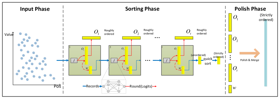
Figure 1. NN-sort architecture

In this section we discuss the design of NN-sort, including challenges and solutions on how to use a neural network model for effective sorting, as well as how such a neural network model can be trained.

Sorting, in essential, is a mapping between two sets of data elements: data before sorted and data after sorted. Therefore, instead of using traditional approaches such as comparing values of different data elements, such mapping can be achieved via a data distribution aware model, which takes a data element as an input and produces its relative location after the whole dataset is sorted as an output. However, there are several challenges in terms of how to make such a model work correctly and effectively. First, for the correctness, this approach must be able to reflect the order among different input data elements precisely. In other words, the results produced by this approach must be the same as those produced by a traditional sorting algorithm. Second, for the effectiveness, the ideal scenario is to find a model that can sort a large volume of input data in one shot. But this is difficult since it requires the model to be complicated and accurate enough to be able to reflect the exact order of all the input data elements. Such a model either consumes enormous training power to train or takes a long time to run during the inference time due to its complexity. Therefore, a trade-off between model accuracy and sorting performance needs to be carefully considered. Third, conflicts are highly possible to occur during the mapping, in which two different input data elements are mapped to the same output. How to effectively deal with such conflicts primarily affects both the correctness and efficiency of this neural network based sorting approach. We will discuss how to tackle these challenges in this section.

3.1. Neural Network Based Sort

Algorithm 1 NN-sort

1:$A$ - array of data points to be sorted

2:$f$ - the learned model.

3:$m$ - the relaxation factor

4:$\tau$ - the threshold of conflicting array size

5:$\epsilon$ - the maximum number of iterations

6:$w$ - the input array of each iteration

7:$o_{i}$ - the array generated by the $i$the iteration to hold the ordered data points

8:$w\leftarrow A$, $O\leftarrow\left[\ \right]$

9:if $w.length>\tau$ then

10:     $i\leftarrow 0$

11:     while $0<i<\epsilon\ \&\&\ w.length>\tau$ do

12:         $Logtis$ $\leftarrow$ $f(w)$

13:         $new\ o_{i}\leftarrow[\infty]*\left(Logits.max*m\right)$

14:         // $c$ holds the conflicting array in each iteration

15:         $c\leftarrow\left[\ \right]$

16:         for $j$ in $Logits.length$ do

17:              $pos\leftarrow round(Logtis[j]*m)$

18:              if $o_{i}[pos]==\infty$ then

19:                  $o_{i}[pos]\leftarrow w[j]$

20:              else $c\leftarrow c\cup w[j]$

21:              end if

22:         end for

23:         // $O$ is an array of roughly sorted arrays from each iteration

24:         $O\leftarrow O\cup o_{i}$

25:         $w\leftarrow c$

26:         ++$i$

27:         $Logits\leftarrow\left[\ \right]$

28:     end while

29:end if

30:$quicksort(w)$

31:return $merge(O,w)$

32:end

We design the neural network based sorting as an iterative approach. Instead of trying to train a complex model and sort all the input data elements in one shot, our approach uses a much simpler model to accomplish the sorting task in multiple rounds. Within each round, the model puts the input data in a roughly sorted order. It is not accurately sorted because the model is not 100% accurate and conflicts may exist in the outputs of the model. When conflicts occur, all the no-conflicts data elements will be organized in an array which is roughly ordered, while the conflicts data elements will be put in another conflicting array, which is used as the input of the next iteration. Such iterations are repeated until the size of the conflicting array becomes smaller than a threshold. Then, the conflicting array is sorted by a traditional sorting approach, such as Quick Sort, As the last step, all the roughly ordered array generated by previous iterations are polished and merged with strictly sorted conflicting array to create the final results. In order to make sure this approach will not run forever in case the model generates large numbers of conflicts, another threshold is used to define the maximum number of iterations this algorithm can go through. A traditional sorting approach will be used to sort the conflicting array and produce the final results when this threashold is reached.

Fig 1 shows the details of this approach. The entire sorting process can be divided into $3$ phases: input phase, sorting phase, polish phase. The input phase is responsible for pre-processing the input data. For instance, converting a string or float type data element into a vector so that it can be consumed by a neural network model. The sorting phase aims at converting unordered data elements into several roughly ordered ones by iteratively running through a model $f$. In our design, specifically, $f$ is a neural network regression model that takes unsorted data elements $\{x_{1},x_{2},..,x_{n}\}$ as input and returns the position of $x_{i}$ (denoted as $round(Logits_{i}*m)$) in an array where all the elements are supposed to be sorted. If conflicts occur, which means different input data elements (i.e., $x_{i},x_{j}$) result in the same output, the conflicting data elements will be stored in the conflicting array $c$ without being ordered, while the non-conflict values are organized in another array $o_{k}$ which is roughly ordered based on the accuracy of the model. In the next iteration, the data elements in $c$ are used as the input of the learned model $f$ again. The size of the conflicting array is checked after each iteration. If it goes below a pre-defined threshold, the conflicting array will not be fed into $f$ again. Instead, it will be sorted using a traditional sorting approach such as Quick Sort, and the result will be stored in $w$. Note that there is a roughly ordered array in the output of each iteration $\{o_{1},o_{2},...,o_{k},...o_{t}\}$ ($t$ is the number of completed iterations and $0<t\leq\epsilon$, in which $\epsilon$ is a pre-defined threshold as the maximum number of iterations). In the polish phase, the final result is created by correcting incorrectly ordered data elements, if there is any, in $\{o_{1},o_{2},....,o_{k},...,o_{t}\}$, and merge them with $w$.

More details of NN-sort workflow is revealed in Algorithm 1. Line 1-23 is correspondent to the sorting phase in while Line 23 reflects the polish phase, and the input phase (i.e., input data pre-processing) is omitted. To begin with, if the size of the input dataset is smaller than the pre-defined threshold $\tau$, a traditional sorting approach will be used. Otherwise, the neural network based sort is invoked. As shown in Algorithm 1, in the first iteration, all the unsorted data elements in the array $A$ are fed into a neural-network model $f$, which returns the $Positions$ array (Lines 4). Element $i$ in this $Positions$ array ($pos_{i}$) represents the relative position of the data points $x_{i}$ in a sorted. In other words, assuming the data needs to be sorted in an increasing order, then the larger the $x_{i}$ is, the bigger $pos_{i}$ is. It worth mentioning that, instead of using $pos_{i}$, which is the direct output of $f$, we use $round(logits_{i}*m)$, which is a rounded value, to represent the position of $x_{i}$. The reasons are as follows. First, the output(i.e., position) of an input data point needs to be an integer, thus $round()$ is used. Second, $m$ is used as the relaxation factor so that the input data elements can be mapped into a larger space, which can effectively reduce the number of conflicts. Line 12 deals with the conflicts when multiple input data elements lead to the same output after being mapped by model $f$. As discussed before, all the conflicting data elements will be put into a conflicting array $c$ and used as the input of $f$ of the next generation. Each iteration ends at line 20, after which a roughly sorted array $o_{i}$ and a conflicting array $c$ are generated. As shown in in line 3, the iterations end when the size of the conflicting array is smaller than a threshold $\tau$. Also notes that if the model $f$ is not working well, this algorithm may not be able to stop since the size of the conflicting array may never become be smaller than $\tau$, which ends up with even larger overhead than traditional sorting algorithms. In order to prevent this from happening, another threshold $\epsilon$ is used to limit the maximum number of iterations. After all the iterations, the last conflicting array $w$ is sorted by traditional sorting algorithms and merged with the leftover arrays $\{o_{1},o_{2},....,o_{k},...,o_{t}\}$.

Algorithm 2 illustrates more details about the polish phase. Roughly ordered arrays $\{o_{1},o_{2},....,o_{k},...,o_{t}\}$ are polish and merged with strictly ordered array $w$ to create the final ordered output $result$. The algorithm goes over all the arrays $o_{i}$ in $O$, and merges them with $w$ one by one. Line 4 - Line 6 removes the null values from the array $o_{i}$. Then, each element in $o_{i}$ and $w$ is iterated, compared, and appended to the $result$(Line8). The time complexity of this appending operation is linear to the size of data element for a given number of iterations in Algorithm 1. Note that $o_{i}$ is a roughly ordered array. Therefore, when an element $a$ is out of order, it needs to be inserted to the correct location in $result$ instead of being appended(Line 10). The cost of $insert$ is higher than $append$, but it is only needed for the out-of-order elements in $o_{i}$. Therefore, the more accurate the model $f$ is, the less overhead the $merge$ has. Our experimental results show that the amount of out-of-order elements created by NN-sort can be negligible, thus the performance of NN-sort is near-linear.

Algorithm 2 merge(O, w)

1:$O$ - an array of arrays, each element $o_{i}$ in $O$ is a roughly ordered array.

2:$w$ - a strictly ordered array.

3:for $o_{i}$ in $O$ do

4:     $result\leftarrow[]$

5:     for $a$ in $o_{i}$ do

6:         if $a==\infty$ then

7:              continue

8:         else

9:              if $a$ is ordered in $o_{i}$ then

10:                  $result$ $\leftarrow$ result.append(min_or_max($a$, $w_{i}$))

11:              else

12:                  $result\leftarrow result.insert(a)$

13:              end if

14:         end if

15:     end for

16:     $w\leftarrow result$

17:end for

18:return $result$

3.2. Example

Fig 2 illustrates a concrete example of how NN-sort works to order a list of unsorted numbers. Given a set of unordered data elements $A=\{32,60,31,1,81,6,88,38,3,59,37,92,91\}$, first of all, NN-sort determines whether the size of $A$ is smaller than a threshold $\tau$. If it is, $A$ will be sorted by a traditional sorting approach. Otherwise, the neural network based sorting is used. In the later scenario, $A$ is first fed into in the sorting phase, in which each data element in $A$ is mapped into the first sparse array denoted by $o_{0}$ via learned model $f$. Note that there is a conflict in the mapping process between data elements $37$ and $38$, since $f$ generates the same result for both data elements. Therefore, the latter one will be stored at a conflicting array $c$. Then, after the first iteration, because the size of $c$ is 5, which is large than $\tau$, and also because the current iteration ID is 1, which is smaller than $\epsilon$, all the data elements in $c$ are fed to the learned model $f$ again for a second iteration, which produce another pair of sorted array $o_{2}$ and conflicting array $c$. After that, since the size of $c$ is smaller than $\tau$, all the data points in $c$ are sorted by a traditional sorting approach such as Quick Sort. Finally, $o_{0}$, $o_{1}$ and $c$ are merged to produce the final result, which is strictly ordered.

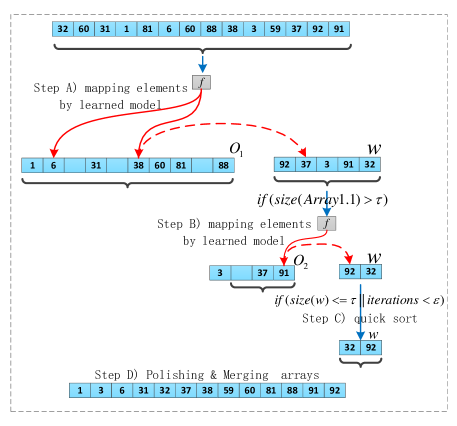
Figure 2. Example

3.3. Training

In this sub-section, we discuss the considerations of how to design and train a model $f$ for NN-sort.

We choose a neural network regression model with 3 hidden layer. The reasons are as following: first, simple neural networks can be efficiently trained using stochastic gradient descent. Also, as shown in our experimental results, such model can converge in less than one to a few passes over the randomized data. Second, to keep the ordering relationship among data element as much as possible, the model $f$ needs to fit into a monotonic function, in which the first derivative has to be, in most of the time, either not smaller than or not larger than 0. If the model is too complicated, overfiting can happen easily, which makes the fitting curves oscillating, which leads to a non-monotonic model. To demonstrate this theory, we observe that when SVR (DBLP:journals/sac/SmolaS04) model is used, 5% of the input data points will be mapped to the wrong place while this problem can be settled after switching to a simple neural network model. In our implementation of NN-sort, the neural network consists of three fully connected layers; the first layer has 32 neurons while the second layer has 8, the third layer has 4 neuron.

(1) $$loss_{\delta}=\left\{\begin{array}[]{lr}\frac{1}{2}(f(x_{i})-label_{i})^{2},&if\ |f(x_{i})-label_{i}|\leq\delta,\\ \delta|f(x_{i})-label_{i}|-\frac{1}{2}\delta^{2},&otherwise\\ \end{array}\right.$$

In order to avoid the impact of outliers during training, model used in this paper is trained according to the Huber loss (Huber, 1964) Eq 1.

4. Model Analysis

Table 1. Notations

symbols	notations
$T_{w}$	the total number of operations in the worst case
$T_{b}$	the total number of operations in the best case
$T_{g}$	the total number of operations in the general case
$n$	the amount of data points to be sorted
$m$	the relaxation factor which can buffer conflicts
$\sigma$	collision rate per iteration
$e_{i}$	the number of data points that were mis-ordered in the $i$-th iteration
$\epsilon$	the preset limit of iterations
$t$	the number of completed iterations
$\theta$	The number of operations required for the data points to pass through the neural network

In this section, we analyze and prove the time complexity of the NN-sort in three cases. The operations required in the sorting process are used as units of analysis. In our design, moving or comparing a elements is considered as an operation. The three cases for analysis are:

• Best case: In this case, the model can sort all the input data elements without incurring any conflict. Therefore, at the end of NN-sort, the conflicting array will be empty, and no traditional sorting algorithm is needed. At same time, the model is accurate enough to not create any out-of-order data element.

• General case: This is the case that lies in between of the best case and the worst case, and it is also the most common one. In this case, the model is able to sort some of the input data elements, but it results in some extent of conflicts, which will be finally resolved by traditional sorting algorithms such as Quick Sort.

• Worst case: In this case, we assume the model incurs an extremely high conflicting rate. Thus it is not helpful at all in sorting. All the input data elements are in the final conflicting array and eventually sorted by a traditional sorting algorithm, such as Quick Sort.

We also provide the cost model, which can help understand the relationship among the conflicting rate, the scale of model $f$, the number iterations, and the amount of data points to be sorted. The notations used in this section are described in Table 1.

4.1. Time Complexity Analysis

4.1.1. Best Case

(2) $$T_{b}(n)=\left\{\begin{array}[]{lr}1,&if\ n=1\\ \theta n+n,&if\ n>1\\ \end{array}\right.$$

In this case, all data elements are ordered after being processed by the neural network model and no traditional sorting algorithm is needed to sort the conflicting array. If $n>1$, it only needs $1$ iteration and $\theta n$ operations to sort all the data elements. It will also need $n$ operations to remove any empty positions at the output array. Therefore, the time complexity of NN-sort in the best case is $O(n)$.

4.1.2. General Case

(3) $$T_{g}(n)=\left\{\begin{array}[]{lr}1,&if\ n=1\\ C^{1}_{g}n+C^{2}_{g}nlogn,&if\ n>1\\ \end{array}\right.$$

$$C^{1}_{g} =\frac{(1-\sigma)+(1-\sigma^{t-1})(\theta+1)}{1-\sigma}$$

(4) $$+\sum_{i=1}^{t}\sigma^{i}n+(1-e_{i})(\sigma^{i-1}-\sigma^{i})+\sigma^{t}log\sigma^{t}$$

(5) $$C^{2}_{g} =\sigma^{t}+e(\sigma^{t}+\sigma^{t-1})$$

In the general case, the whole sorting process can be divided into 2 parts:

• generating several roughly ordered arrays and one ordered conflicting array, which denoted as $s_{g}(n)$. (corresponding to ’Sorting phase’)

• merging all the roughly ordered arrays,which denoted as $p_{g}(n)$. ( corresponding to ’Polish phase’)

$s_{g}(n)$ consists of two kinds of operations which are iteratively feding the data elements into learned model $f$ and sorting the last conflicting array (operations is about $\sigma^{t}nlog\sigma^{t}n$) using traditional sorting algorithms such as Quick Sort. As shown in Proof 4.1.2, if $n>1$, each iteration produces $\theta n+n$ operations and the next iteration is going to deal with $\sigma n$ data elements. $\sum_{i=0}^{t-1}\sigma^{i}(\theta n+n)$ operations need to be carried out at the end of the $t$-th iteration ($0<t\leq\epsilon$). Moreover, to sort the last conflicting array, another $\sigma^{t}nlog\sigma^{t}n$ operations are needed by Quick Sort. Therefore the total operations of $s_{g}(n)$ is $\sum_{i=0}^{t-1}\sigma^{i}(\theta n+n)+\sigma^{t}nlog\sigma^{t}n$.

$p_{g}(n)$ consists of two procedures: correcting the out-of-order data elements produced by the model and merging the ordered arrays. For ordered arrays, NN-sort only needs to traverse these arrays to complete the merge process ($O(1)$ complexity). There are always $\sigma^{i}n$ strictly ordered data elements in the last conflicting array and $\sum_{i=1}^{t}\sigma^{i}n+(1-e_{i})(\sigma^{i-1}-\sigma^{i})n$ strictly ordered data elements produced by the model. Thus, the total number of operations of $p_{g}(n)$ in $i$-th iterations is $\sigma^{i}n+\sum_{i=1}^{t}\sigma^{i}n+(1-e_{i})(\sigma^{i-1}-\sigma^{i})n$. To order the out-of-order data elements, NN-sort needs to correct them by inserting these data elements into a strictly ordered array. It takes $e_{i}(\sigma^{i-1}-\sigma^{i})nlogn$ operations to process $e_{i}(\sigma^{i-1}-\sigma^{i})n$ out-of-order data elements. Therefore, the amount of operations of NN-sort in general case is $\sum_{i=0}^{t-1}\sigma^{i}(\theta n+n)+\sigma^{t}nlog\sigma^{t}n+[\sigma^{t}+e_{i}(\sigma^{t}+\sigma^{t-1})]nlogn$. As $e_{i}\in(0,1)$, $\sigma_{i}\in(0,1)$, and both $\theta$ and $t$ can be considered as constants the time complexity is $O(nlogn)$. Note that the number of operations can be controlled by $t$ and $\theta$. The fewer the out-of-order elements are and the lower the conflicting rate is, the closer the NN-sort complexity is to linear.

Proof.

$$T_{g}(n) ={s_{g}}(n)+p_{g}(n)\text{\ , (n>1)}$$

$$=\sum_{i=0}^{t-1}\sigma^{i}(\theta n+n)+\sigma^{t}nlog(\sigma^{t}n)+p_{g}(n)$$

$$=\sum_{i=0}^{t-1}\sigma^{i}(\theta n+n)+\sigma^{t}nlog(\sigma^{t}n)$$

$$+\sum_{i=1}^{t}\sigma^{i}n+(1-e_{i})(\sigma^{i-1}-\sigma^{i})n+e_{i}(\sigma^{i-1}-\sigma^{i})nlogn$$

$$=\frac{(1-\sigma)+(1-\sigma^{t-1})(\theta+1)}{1-\sigma}n+\sigma^{t}nlog\sigma^{t}n$$

$$+\sum_{i=1}^{t}\sigma^{i}n+(1-e_{i})(\sigma^{i-1}-\sigma^{i})n+e_{i}(\sigma^{i-1}-\sigma^{i})nlogn$$

$$=[\frac{(1-\sigma)+(1-\sigma^{t-1})(\theta+1)}{1-\sigma}$$

$$+\sum_{i=1}^{t}\sigma^{i}n+(1-e_{i})(\sigma^{i-1}-\sigma^{i})+\sigma^{t}log\sigma^{t}]n$$

(6) $$+[\sigma^{t}+e_{i}(\sigma^{t}+\sigma^{t-1})]nlogn$$

∎

4.1.3. Worst Case

(7) $$T_{w}(n)=\left\{\begin{array}[]{lr}1,&if\ n=1\\ \theta\times\epsilon\times n+2nlogn,&if\ n>1\\ \end{array}\right.$$

The sorting process in this case can be divided into 3 parts:

• feeding data elements into model for $\epsilon$ times.

• sorting all the conflicting data points.

• correcting the out-of-order data elements and merging all the sorted arrays.

In this case, we suppose model $f$ does not help at all for sorting. Therefore, in each iteration, only one data element is mapped to a roughly ordered array $o$, and the rest of data elements are mapped to the conflicting array. This means almost all the data elements should be sorted by traditional sorting algorithm (about $nlogn$ opeartions). Moreover, it still requires a $\theta\times n$ operations to feed data elements into model $f$ for $\epsilon$ times , as well as $tnlogn$ opeartions to insert data elements from the roughly ordered arrays into the final sorted result. Hence, in the worst case, the NN-sort needs $\theta\times\epsilon\times n+2nlogn$ operations to sort $n$ data elements and the complexity is $O(nlogn)$.

4.2. Cost Model

A more complex neural network usually means stronger model expression expressivity, lower conflicting rate, and higher inferencing costs, and vise versa. There is a need to find a balance among these factors to achieve the best NN-sort performance. Therefore, in this subsection, we provide a cost model that helps explain the relationship among conflicting rate $\sigma$, the scale of neural network $\theta$, the number of iterations $t$.

In some cases, the user may require that the number of operations of NN-sort takes no more than Quick Sort ($nlogn$). Therefore, we introduce a cost model represented by Eq 8 to determine what should be the values of the $\sigma,t,\theta,n$ to make NN-sort perform no worse than Quick Sort. The proof is shown in Proof 4.2.

(8) $$n>e^{\frac{C^{1}_{g}}{1-C^{2}_{g}}}$$

Proof.

$$nlogn> T_{g}(n)$$

$$1> \frac{T_{g}(n)}{nlogn}$$

$$1> \frac{C_{g}^{1}}{logn}+C^{2}_{g}$$

(9) $$n> e^{\frac{C^{1}_{g}}{1-C^{2}_{g}}}$$

∎

It can be observed that when the values of $\sigma$, $t$ and $\theta$ are selected in a way that makes $n>e^{\frac{C^{1}_{g}}{1-C^{2}_{g}}}$, the number of operations to sort an array of size $n$ by NN-sort is smaller than $nlogn$, which is the lower bound of the traditional sorting algorithms. In fact, if the model $f$ is accurate enough(i.e $\sigma<0.3$ or $e_{i}<0.2$), the number of sorting operations should be closer to $n$

5. Evaluation

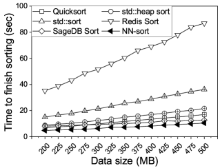
(a) Log-normal

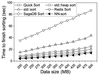
(b) Normal

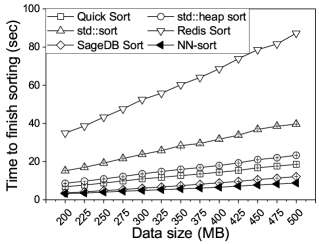
(c) Uniform

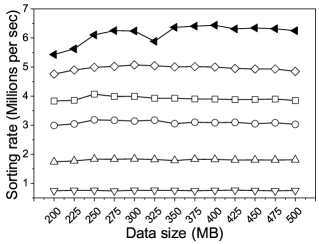
(d) Log-normal

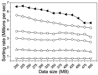
(e) Normal

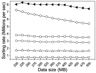
(f) Uniform

Figure 3. Performance of NN-sort on dataset with different distributions

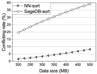
(a) Log-normal

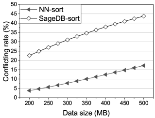
(b) Normal

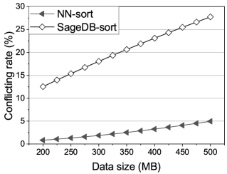
(c) Uniform

Figure 4. Comparison of conflicting rate between NN-sort and SageDB Sort under different data distributions

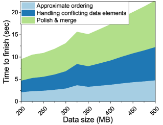
(a) Log-normal

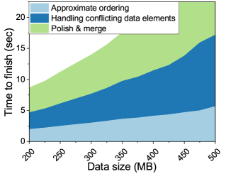
(b) Normal

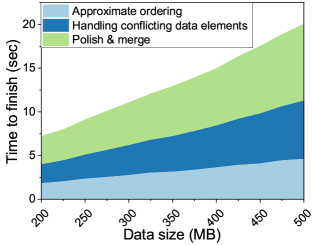
(c) Uniform

Figure 5. The performance of each step

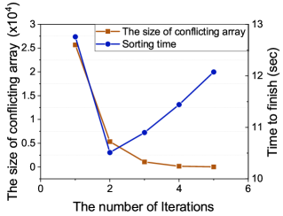
(a) Log-normal

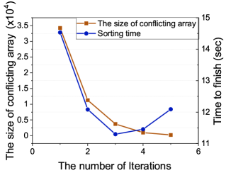
(b) Normal

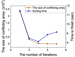
(c) Uniform

Figure 6. Evaluation of the impact of iterations

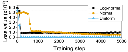
(a) Data size: 100MB

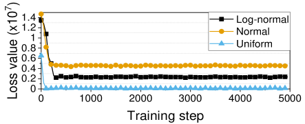
(b) Data size: 200MB

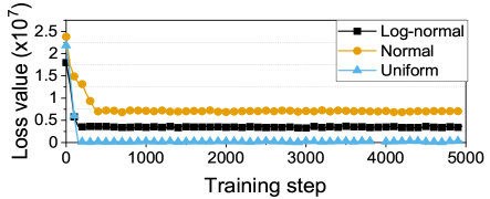
(c) Data size: 300MB

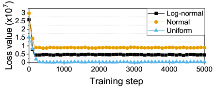
(d) Data size: 400MB

Figure 7. Evaluation of the training time & training steps

In this section, we evaluate and analyze the performance of NN-sort by using different datasets. The datasets used in this section are generated from the most common observed distributions in the real world, such as uniform distribution, normal distribution, and log-normal distribution. The size of every dataset varies from 200 MB to 500 MB and each data element is 64 bits wide. The performance between NN-sort and the following representative traditional sorting algorithms are compared:

• Quick Sort(Cormen, [n. d.]): This algorithm divides the input dataset into two independent partitions, such that all the data elements in the first partition is smaller than those in the second partition. Then, the dataset in each partition is sorted recursively. The execution time complexity of Quick Sort can achieve $O(nlogn)$ in the best case while $O(n^{2})$ in the worst case.

• std::sort(C++, [n. d.]): std::sort is one of the sorting algorithms from c++ standard library, and its time complexity is approximately $O(nlogn)$

• std::heap sort(C++, [n. d.]): std::heap sort is another sorting algorithm from c++ standard library, and it guarantees to perform at $O(nlogn)$ complexity.

• Redis Sort(Red, [n. d.]): Redis Sort is a $sortSet$ based sorting method, in which $sortSet$ is a data structure. To sort $M$ data points in a $sortSet$ of size $N$, the efficiency of Redis Sort is $O(N+M*log(M))$.

• SageDB Sort(Kraska et al., 2019): The basic idea of SageDB Sort is to speed up sorting by using an existing cumulative distribution function model to organize the data elements in roughly sorted order, and then use traditional sorting algorithms to sort the data points that are out of order. Unlike our work, SageDB Sort maps data points only once, which results in higher conflicting rate thus lower sorting efficiency.

The experiments are carried out on a machine with 64GB main memory and a 2.6GHZ Intel(R) i7 processor. The machine uses RedHat Enterprise Server 6.3 as its operating system. Each number shown here is the median of ten independent runs.

5.1. Sorting Performance

Fig 3 compares the efficiency of NN-sort with the other traditional sorting algorithms by using different datasets with increasing sizes. The total sorting time is shown in Fig 3(a) - Fig 3(c), the sorting rate is displayed in Fig 3(f) - Fig 3(f), while Fig 3(e) and Fig 3(f) shows the conflicting rate.

It is clear to observe that NN-sort has significant performance benefits over the traditional sorting algorithms. For example, Fig 3(d) reveals that, for the log-normal distribution dataset, the sorting rate of NN-sort is almost 8300 data elements per second, which is 2.8 times of std::heap sort, 10.9 times of Redis Sort, 4.78 times of std::sort, 218% higher than Quick Sort, and also outperforms SageDB Sort by 15%. Fig 3(e) and Fig 3(f) compares the conflicting rate, which is represented by the number of data elements touched by the traditional sorting algorithm divided by those touched by NN-sort, in NN-sort and SageDB Sort. Since additional mapping operations are needed to deal with the conflicts, this also explains why NN-sort performs consistently better.

5.2. Sorting Performance Breakdown

More details of NN-sort performance are measured, and the results are shown in Fig 5. The execution time of NN-sort is broken down into three components:

• Approximate ordering: the time taken to make the input data elements roughly ordered. This step includes the time of pre-processing and also generating the first ordered array and the first conflicting array.

• Handing conflicts: the time taken to deal with conflicts. This step includes ordering the data elements in the conflicting array, which is generated by the previous step. In fact, this step includes all the iterations in Algorithm 1 except the first one.

• Merging: this step is correspondent to the merge operation, which corrects the out-of-order data elements and merges all the previous ordered arrays to generate the final strictly orderered output.

Fig 5 shows that the time NN-sort takes to produce a roughly ordered array is stable, and the data distribution(including both training data and sorting data) will affect the time to finish sorting. As shown in Fig 5(b), NN-sort spends longer time on sorting dataset with normal distribution, since more conflicts are created in this scenario. Therefore, the fewer conflicts per iteration, the better NN-sort can perform.

5.3. Impact of Iterations

The sorting performance will be affected by the size of the last conflicting array and the number of iterations. If the number of iteration increases, the number of data elements that needs to be sorted using traditional methods will decrease, but the time spent on running the model will become longer due to more iterations. On the contrary, if the number of iterations is reduced, the size of the conflicting array can be large, which takes a long time to use the traditional sorting algorithm to sort. In this set of experiments, we quantify how these two factors can affect the performance of NN-sort, so that to provide a guide to practitioners or researchers to make a more informed decision on how to achieve the best performance of NN-sort.

In Fig 6, the yellow line represents the size of the last conflicting array; the blue line illustrates the sorting time. It shows that the more iterations, the smaller the size of the last conflicting array is. However, this does not mean that the more iterations, the better sorting performance is, because each iteration needs to invoke the model multiple times, which equals to the number of input data elements. It can be obtained that, in our experiments, $2-3$ times of iterations are good enough.

5.4. Training Time

Model $f$, either shallow neural networks or even simple linear regression models, can be trained relatively fast. In this sub-section, we evaluate the training time and the value of the loss. We trained a three-layer, fully connected neural network with 32, 8, and 4 neurons in each layer, respectively. ReLU(DBLP:conf/iwaenc/XuCL16) is used as the activation function and Adadelta(DBLP:journals/corr/abs-1212-5701) is applied as the optimizer in Tensorflow (Abadi et al., 2016). The data elements are the input features, while the positions of these data elements in the sorted array are the labels. We evaluate the convergence time and loss value Eq 1 of model $f$ under three kinds of data distributions (Log-normal, Normal, and Uniform) with 4 training data sizes(100MB, 200MB, 300MB, 400MB).

In Fig 7, the X-axis represents the training step, while the Y-axis displays the changes in the loss value. There are several interesting observations. First, the training process can be finished in a short time. For example, it only takes 8.55 seconds to train a model using 100MB uniformly distributed data elements, and 3.71 seconds to train a model using 100MB log-normal distributed data elements. Even training a model using 400MB data elements takes no more than 10 seconds. Second, models trained by different distributions have similar converge rates, although they converge to different values. For instance, when the data size is 400MB, model trained by uniform distributed data takes about 500 steps to converge to a loss value of $1*10^{6}$; For normally distributed data, it takes about 250 steps to converge to a loss value of $5*10^{6}$; While for uniformly distributed data, it takes about 200 steps to converge in loss value of $7*10^{6}$.

5.5. Impact of Data Distribution

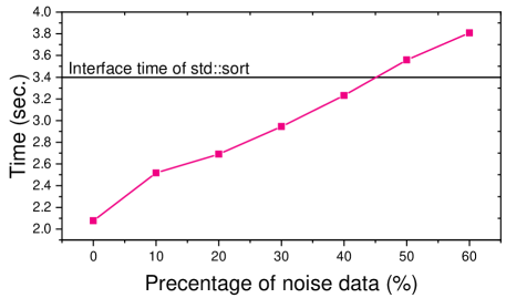
Figure 8. The impact of data distribution on NN-sort

As shown in the previous experiments, NN-sort works well when the sorting data is in the same distribution as the training data. A natural question to ask is what if the sorting data has a different distribution than the training data. To answer this question, we trained a model by using a dataset which contains 100MB uniformed distributed data elements. Then, we use this model to sort datasets with difference distributions. Specifically, the sorting dataset is a mix of data with both uniformed and normal distributions, and we denote the of normal distribution data as noisy data. The sorting time is measured to reflect the effectiveness of NN-sort and the results are displayed in Figure 8. On one hand, it is expected that the effectiveness of NN-sort decreases as the dataset becomes more noisy. This is because when the distribution similarity between the training data and sort data increases, more out-of-order data elements are produced by NN-sort, which need to be eventually sorted by traditional sorting algorithms in the polish phase. On the other hand, even when comparing with one of the fastest and widely used sorting algorithm std::sort, NN-sort still outperforms it with up to 45% noisy data.

5.6. Real-wrod Dataset

Table 2. Evaluation under real-world data

Algorithms	Sorting time (sec.)	Sorting Rate (No. of Data Points/sec)	Conflict rate (%)
quicksort	$10.86$	$4666.14$	-
std::heap sort	$13.46$	$3746.44$	-
std::sort	$23.71$	$2127.19$	-
Redis::sort	$63.14$	$798.6320$	-
SageDB-sort	$10.53$	$4790.125$	$9.16$
NN-sort	$8.47$	$5950.186$	$0.4$

To verify the performance of the NN-sort under the real-world dataset. We use the QuickDraw game dataset from Google Creative Lab(Google, [n. d.]), which consists of $50,426,265$ records and each records has 6 properties: ’key-id’, ’word’, ’country code’, ’timestamp’, ’recognized’, ’drawing’. The model used in this set of experiments is the one that is trained in previous subsections under uniformly distributed data.

As shown in Table 2, NN-sort shows a significant performance benefits over traditional sorting under real-world data. In terms of the sorting rate, NN-sort is 5950 per second, which is 2.72 times of std::sort and 7.34 times of Redis Sort. It is also 58% faster than std::heap sort. We can also observe that NN-sort outperforms SageDB Sort in terms of both conflicting rate and sorting rate.

6. Conclusions and Future Work

Sorting is wildly used in many computation tasks, such as database applications and big data processing jobs. We have presented NN-sort, a neural network based and data distribution aware sorting method. NN-sort uses a model trained on historical data to sort the future data. NN-sort employs multiple iterations to reduce the conflicts during the sorting process, which is observed as the primary performance bottleneck in using DNN models to solve the sorting problems. We also provide a comprehensive analysis of the NN-sort algorithm, including the bound of its complexity, the cost model to describe how to find the right balance among different factors, such as the model accuracy and sorting performance. Experimental results demonstrate that NN-sort outperforms traditional sorting algorithms by up to 10.9x. By following this thread of research, we are investigating how such approach can be effectively applied to applications, such as MapReduce jobs and big data analytics engines, to improve the performance of their sorting phase, which can eventually benefit the overall effectiveness of the application or system.

References

- (1)
- C++ ([n. d.]) [n. d.]. C++ Resources Network. http://www.cplusplus.com/. General information about the C++ programming language, including non-technical documents and descriptions.
- Pyt ([n. d.]) [n. d.]. Python Resources Network. https://www.python.org/. General information about the Python programming language, including non-technical documents and descriptions.
- Red ([n. d.]) [n. d.]. Redis. https://redis.io/. Redis is an open source (BSD licensed), in-memory data structure store, used as a database, cache and message broker.
- Abadi et al. (2016) Martín Abadi, Paul Barham, Jianmin Chen, Zhifeng Chen, Andy Davis, Jeffrey Dean, Matthieu Devin, Sanjay Ghemawat, Geoffrey Irving, Michael Isard, Manjunath Kudlur, Josh Levenberg, Rajat Monga, Sherry Moore, Derek Gordon Murray, Benoit Steiner, Paul A. Tucker, Vijay Vasudevan, Pete Warden, Martin Wicke, Yuan Yu, and Xiaoqiang Zheng. 2016. TensorFlow: A System for Large-Scale Machine Learning. In 12th USENIX Symposium on Operating Systems Design and Implementation, OSDI 2016, Savannah, GA, USA, November 2-4, 2016. 265–283. https://www.usenix.org/conference/osdi16/technical-sessions/presentation/abadi
- Andersson et al. (1998) Arne Andersson, Torben Hagerup, Stefan Nilsson, and Rajeev Raman. 1998. Sorting in linear time? J. Comput. System Sci. 57, 1 (1998), 74–93.
- Arkhipov et al. (2017) Dmitri I. Arkhipov, Di Wu, Keqin Li, and Amelia C. Regan. 2017. Sorting with GPUs: A Survey. CoRR abs/1709.02520 (2017). arXiv:1709.02520 http://arxiv.org/abs/1709.02520
- Bandyopadhyay and Sahni (2010) Shibdas Bandyopadhyay and Sartaj Sahni. 2010. GRS - GPU radix sort for multifield records. In 2010 International Conference on High Performance Computing, HiPC 2010, Dona Paula, Goa, India, December 19-22, 2010. 1–10. https://doi.org/10.1109/HIPC.2010.5713164
- Brockmann et al. (2006) Dirk Brockmann, Lars Hufnagel, and Theo Geisel. 2006. The scaling laws of human travel. Nature 439, 7075 (2006), 462.
- Buss and Knop (2019) Sam Buss and Alexander Knop. 2019. Strategies for stable merge sorting. In Proceedings of the Thirtieth Annual ACM-SIAM Symposium on Discrete Algorithms. Society for Industrial and Applied Mathematics, 1272–1290.
- Cederman and Tsigas (2008a) Daniel Cederman and Philippas Tsigas. 2008a. On sorting and load balancing on GPUs. SIGARCH Computer Architecture News 36, 5 (2008), 11–18. https://doi.org/10.1145/1556444.1556447
- Cederman and Tsigas (2008b) Daniel Cederman and Philippas Tsigas. 2008b. A Practical Quicksort Algorithm for Graphics Processors. In Algorithms - ESA 2008, Dan Halperin and Kurt Mehlhorn (Eds.). Springer Berlin Heidelberg, Berlin, Heidelberg, 246–258.
- Cederman and Tsigas (2009) Daniel Cederman and Philippas Tsigas. 2009. GPU-Quicksort: A practical Quicksort algorithm for graphics processors. ACM Journal of Experimental Algorithmics 14 (2009). https://doi.org/10.1145/1498698.1564500
- Chlebus (1988) Bogdan S. Chlebus. 1988. A Parallel Bucket Sort. Inf. Process. Lett. 27, 2 (1988), 57–61. https://doi.org/10.1016/0020-0190(88)90092-0
- Cook and Shane ([n. d.]) Cook and Shane. [n. d.]. CUDA programming: A developer’s guide to parallel computing with GPUs. Morgan Kaufmann Publishers.
- Cormen ([n. d.]) Thomas H. Cormen. [n. d.]. Introduction to Algorithms, 3rd Edition. Press.
- Davidson et al. (2012) Andrew Davidson, David Tarjan, Michael Garland, and John D. Owens. 2012. Efficient Parallel Merge Sort for Fixed and Variable Length Keys. In Innovative Parallel Computing.
- de Gouw et al. (2014) Stijn de Gouw, Frank S. de Boer, and Jurriaan Rot. 2014. Proof Pearl: The KeY to Correct and Stable Sorting. J. Autom. Reasoning 53, 2 (2014), 129–139. https://doi.org/10.1007/s10817-013-9300-y
- de Gouw et al. (2016) Stijn de Gouw, Frank S. de Boer, and Jurriaan Rot. 2016. Verification of Counting Sort and Radix Sort. In Deductive Software Verification - The KeY Book - From Theory to Practice. 609–618. https://doi.org/10.1007/978-3-319-49812-6_19
- Dean and Ghemawat (2008) Jeffrey Dean and Sanjay Ghemawat. 2008. MapReduce: simplified data processing on large clusters. Commun. ACM 51, 1 (2008), 107–113. https://doi.org/10.1145/1327452.1327492
- Edelkamp and Weiß (2014) Stefan Edelkamp and Armin Weiß. 2014. QuickXsort: Efficient Sorting with n logn - 1.399n + o(n) Comparisons on Average. In Computer Science - Theory and Applications - 9th International Computer Science Symposium in Russia, CSR 2014, Moscow, Russia, June 7-11, 2014. Proceedings. 139–152. https://doi.org/10.1007/978-3-319-06686-8_11
- Edelkamp and Weiß (2019) Stefan Edelkamp and Armin Weiß. 2019. Worst-Case Efficient Sorting with QuickMergesort. In Proceedings of the Twenty-First Workshop on Algorithm Engineering and Experiments, ALENEX 2019, San Diego, CA, USA, January 7-8, 2019. 1–14. https://doi.org/10.1137/1.9781611975499.1
- Faghri et al. (2012) Faraz Faghri, Sobir Bazarbayev, Mark Overholt, Reza Farivar, Roy H. Campbell, and William H. Sanders. 2012. Failure Scenario As a Service (FSaaS) for Hadoop Clusters. In Proceedings of the Workshop on Secure and Dependable Middleware for Cloud Monitoring and Management (SDMCMM ’12). ACM, New York, NY, USA, Article 5, 6 pages. https://doi.org/10.1145/2405186.2405191
- Galakatos et al. (2019) Alex Galakatos, Michael Markovitch, Carsten Binnig, Rodrigo Fonseca, and Tim Kraska. 2019. FITing-Tree: A Data-aware Index Structure. In Proceedings of the 2019 International Conference on Management of Data, SIGMOD Conference 2019, Amsterdam, The Netherlands, June 30 - July 5, 2019. 1189–1206. https://doi.org/10.1145/3299869.3319860
- Google ([n. d.]) Google. [n. d.]. Google Creative Lab. Available: https://github.com/googlecreativelab. Google Creative Lab [Online].
- Graefe (2006) Goetz Graefe. 2006. Implementing sorting in database systems. ACM Comput. Surv. 38, 3 (2006), 10. https://doi.org/10.1145/1132960.1132964
- Han (2002) Yijie Han. 2002. Deterministic sorting in O (n log log n) time and linear space. In Proceedings of the thiry-fourth annual ACM symposium on Theory of computing. ACM, 602–608.
- Han and Thorup (2002) Yijie Han and Mikkel Thorup. 2002. Integer sorting in O (n/spl radic/(log log n)) expected time and linear space. In The 43rd Annual IEEE Symposium on Foundations of Computer Science, 2002. Proceedings. IEEE, 135–144.
- Hilker et al. (2012) Rolf Hilker, Corinna Sickinger, Christian N.S. Pedersen, and Jens Stoye. 2012. UniMoG—a unifying framework for genomic distance calculation and sorting based on DCJ. Bioinformatics 28, 19 (07 2012), 2509–2511. https://doi.org/10.1093/bioinformatics/bts440 arXiv:http://oup.prod.sis.lan/bioinformatics/article-pdf/28/19/2509/812322/bts440.pdf
- Huber (1964) Peter J. Huber. 1964. Robust Estimation of a Location Parameter. Annals of Mathematical Statistics 35, 1 (1964), 73–101.
- Jiang and Jia (2011) Bin Jiang and Tao Jia. 2011. Exploring human mobility patterns based on location information of US flights. arXiv preprint arXiv:1104.4578 (2011).
- Kirkpatrick and Reisch (1983) David Kirkpatrick and Stefan Reisch. 1983. Upper bounds for sorting integers on random access machines. Theoretical Computer Science 28, 3 (1983), 263–276.
- Kraska et al. (2019) Tim Kraska, Mohammad Alizadeh, Alex Beutel, Ed H. Chi, Ani Kristo, Guillaume Leclerc, Samuel Madden, Hongzi Mao, and Vikram Nathan. 2019. SageDB: A Learned Database System. In CIDR 2019, 9th Biennial Conference on Innovative Data Systems Research, Asilomar, CA, USA, January 13-16, 2019, Online Proceedings. http://cidrdb.org/cidr2019/papers/p117-kraska-cidr19.pdf
- Kraska et al. (2018) Tim Kraska, Alex Beutel, Ed H. Chi, Jeffrey Dean, and Neoklis Polyzotis. 2018. The Case for Learned Index Structures. In Proceedings of the 2018 International Conference on Management of Data, SIGMOD Conference 2018, Houston, TX, USA, June 10-15, 2018. 489–504. https://doi.org/10.1145/3183713.3196909
- Leischner et al. (2010) Nikolaj Leischner, Vitaly Osipov, and Peter Sanders. 2010. GPU sample sort. In 24th IEEE International Symposium on Parallel and Distributed Processing, IPDPS 2010, Atlanta, Georgia, USA, 19-23 April 2010 - Conference Proceedings. 1–10. https://doi.org/10.1109/IPDPS.2010.5470444
- Li et al. (2019) Xiaoming Li, Hui Fang, and Jie Zhang. 2019. Supervised User Ranking in Signed Social Networks. In The Thirty-Third AAAI Conference on Artificial Intelligence, AAAI 2019, The Thirty-First Innovative Applications of Artificial Intelligence Conference, IAAI 2019, The Ninth AAAI Symposium on Educational Advances in Artificial Intelligence, EAAI 2019, Honolulu, Hawaii, USA, January 27 - February 1, 2019. 184–191. https://aaai.org/ojs/index.php/AAAI/article/view/3784
- Mitzenmacher (2019) Michael Mitzenmacher. 2019. A Model for Learned Bloom Filters, and Optimizing by Sandwiching. CoRR abs/1901.00902 (2019). arXiv:1901.00902 http://arxiv.org/abs/1901.00902
- Musser (1997) David R. Musser. 1997. Introspective Sorting and Selection Algorithms. Softw., Pract. Exper. 27, 8 (1997), 983–993.