Radio Frequency Fingerprint Identification Based on Denoising Autoencoders

Abstract

Radio Frequency Fingerprinting (RFF) is one of the promising passive authentication approaches for improving the security of the Internet of Things (IoT). However, with the proliferation of low-power IoT devices, it becomes imperative to improve the identification accuracy at low SNR scenarios. To address this problem, this paper proposes a general Denoising AutoEncoder (DAE)-based model for deep learning RFF techniques. Besides, a partially stacking method is designed to appropriately combine the semi-steady and steady-state RFFs of ZigBee devices. The proposed Partially Stacking-based Convolutional DAE (PSCDAE) aims at reconstructing a high-SNR signal as well as device identification. Experimental results demonstrate that compared to Convolutional Neural Network (CNN), PSCDAE can improve the identification accuracy by 14% to 23.5% at low SNRs (from -10 dB to 5 dB) under Additive White Gaussian Noise (AWGN) corrupted channels. Even at SNR = 10 dB, the identification accuracy is as high as 97.5%.

I Introduction

Nowadays, the Internet of things (IoT) is becoming more and more ubiquitous in our everyday lives. IoT integrates physical devices into the core networks to allow them to communicate with each other and offer efficient services. However, with the deployment of IoT networks, various security risks have emerged as IoT devices can provide and/or have access to private information. One of the profound security challenges in IoT networks is identity authentication, which is the first line of defense against intruders. Identity vulnerabilities in the IoT networks contain these main facets as follows. First, cryptographic keys or certificates cannot be efficiently distributed due to the limited computing power leading to weak authentication [1]. Second, default keys or credentials can be brute-forced by high-computing-power attackers, extracted from device firmware or mobile apps, or intercepted at login [2]. Third, the ID number such as MAC address in the header needs extra spectral or power resources, which is limited in IoT applications, to be transmitted [3]. Hence, a passive authentication mechanism without cryptographic materials or IDs may be the future of IoT identity authentication.

Radio Frequency Fingerprinting (RFF) is a promising passive authentication technique to identify transmitters by extracting device-specific features/fingerprints from Radio Frequency (RF) signals. RFF is the inherent attribute of the device’s hardware variability in the RF frontend [4]. It is unique for each transmitter and is arduous to impersonate. A lot of research has been executed in this area since the 1990s. Traditional RFF methods can be grouped into transient approaches and steady-state approaches based on their target signal region. More recently, some studies have embraced Deep Learning (DL) for RFF identification. These existing DL RFF techniques all belong to steady-state approaches. In these approaches, minimal preprocessing is carried out on the down-converted baseband signals and then sent to Neural Networks (NNs) for feature extraction and classification [5]. Nevertheless, depending on the input type of NN, DL RFF techniques can be further categorized into Time-series-based DL RFFs (TDL RFFs) and Image-based DL RFFs (IDL RFFs).

TDL RFFs always adopt baseband In-phase/Quadrature (I/Q) samples, which are concatenated in one channel or separate in I/Q channels, as the network input. In [6], MultiLayer Perceptron (MLP) and Convolutional Neural Network (CNN) were applied to each symbol alone to discern 22 LoRa devices. Subsequently, Merchant et al. input the time-domain complex baseband error signal to a CNN to identify seven ZigBee devices against primary user emulation attacks in cognitive radio networks [7]. Long Short Term Memory (LSTM) was also used to learn higher-order correlations between the signal samples to identify USRPs [8]. In [4], a multi-sampling CNN was proposed to extract multi-scale features from the well-synchronized preambles for discerning 54 ZigBee devices.

In IDL RFFs, time series are further transformed to images based on various techniques before feeding into networks. To name only a few, Recurrence Plot (RP), Continuous Wavelet Transform (CWT), Short-Time Fourier Transform (STFT), and Hilbert Transform (HT) have been employed to generate images. After transforming, these images were sent to a deep network such as CNN, Deep Neural Network (DNN), Deep Residual Network (DRN), or Multi-Stage Training (MST) for feature extraction and transmitter identification [9, 10, 11, 12].

Although various DL RFFs have been demonstrated to achieve excellent identification in high SNR regions, their performance in low SNRs is far from satisfactory. For instance, at SNR = 10 dB, the classification accuracies were only 73.73% for seven ZigBee devices [7], 38% for 12 mobile phones [9], 58% for seven USRPs [13], and 65% for five simulated radio emitters [12], respectively. However, since most of the IoT devices are battery-powered, the transmitting power is relatively low, they usually need to work in low SNR scenarios. Therefore, it has a practical significance to study DL RFFs in low SNR scenarios.

To overcome these shortcomings, this paper proposes a general DL model based on Denoising AutoEncoder (DAE) and a dedicated partially stacking method for ZigBee devices. First, we perform synchronization and compensation on the received ZigBee baseband signals. Then the steady-state symbols in the preamble are stacked and concatenated to the semi-steady preamble symbols. Thereafter, we propose a Convolutional Denoising AutoEncoder (CDAE)-based network to extract fingerprints from these concatenated symbols for identifying 27 Ti CC2530 ZigBee devices.

The main contributions are summarized as follows:

• We propose a universal DAE-based architecture for all the DL RFF techniques to enhance their performance, especially at low and medium SNRs. Our DAE-based approach can be trained by jointly minimizing the reconstruction error and the classification loss.

• Inspired by stacking spread sequences to enhance SNR [14], we partially stack the steady-state symbols in the ZigBee preamble rather than stack all the preamble symbols. Partially stacking and concatenation are efficient for combining the semi-steady RFF and the steady-state RFF.

• We further investigate the performance of our proposed Partially Stacking-based CDAE (PSCDAE) approach by selecting two convolutional layers as the encoder of CDAE and a dense layer with Softmax as the classifier. Simulation results demonstrate that the proposed PSCDAE outperforms the original CNN method under all training scenarios. When identifying 27 ZigBee devices, it achieves an accuracy of 97.5% even at SNR = 10 dB.

The remainder of this paper is organized as follows. Section II introduces the novel DAE-based DL RFF approach. Section III discusses the partially stacking method for ZigBee devices. Section IV shows the performance evaluation of the proposed scheme. Finally, Section V concludes this paper.

II RFF Based on Denoising Autoencoders

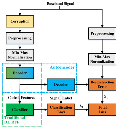
Figure 1: Denoising AutoEncoder-based DL RFF architecture.

An AutoEncoder (AE) is a neural network designed to learn high-level data representation by the encoder and reconstruct the input from that representation by the decoder in an unsupervised manner [15]. By introducing input corruption such as masking noise, effective features relatively stable and robust to the corruption can be extracted by DAE [16]. However, AE is generally used for pretraining and initialization of classification networks. Here, we propose a novel DAE-based DL RFF approach, in which the encoder, decoder, and classifier are trained simultaneously, as shown in Fig. 1. It is worth noting that a conventional DL RFF method only includes an encoder for feature extraction and a classifier for identification without a decoder for reconstruction.

Assume the received baseband signal $\mathbf{s}$ in the training is ideal, which means there is no external wireless channel. It can be denoted as

$$\mathbf{s}=RFF(\mathbf{x}),$$ (1)

where the mathematical function $RFF(\cdotp)$ represents the device fingerprint, and $\mathbf{x}$ is the transmitted data. Then we will first corrupt the input $\mathbf{s}$ to simulate the channel influence as

$$\tilde{\mathbf{s}}=H(\mathbf{s}),$$ (2)

where $H(\cdotp)$ can be an Additive White Gaussian Noise (AWGN) channel or a multipath channel. Thereafter, various preprocessing approaches including synchronization, frequency and phase offset compensation [17], and transforms (CWT, STFT, HT, etc.) can be applied to the corrupted signal:

$$\mathbf{s^{\prime}}=Pre(\tilde{\mathbf{s}}),$$ (3)

where $Pre(\cdotp)$ denotes the preprocessing. Its output $\mathbf{s^{\prime}}$ can be either a time series or an image, thus our method fits for TDL RFFs and IDL RFFs. Additionally, a min-max normalization is indispensable, since the output of the decoder introduced later is always between 0 and 1. The minimum and maximum values in each dimension of the preprocessed vector $\mathbf{s^{\prime}}$ in the training dataset are used and saved for the min-max normalization:

$$\begin{split}\mathbf{z}=&\>min\_max\_norm(\mathbf{s^{{}^{\prime}}})\\ =&\>\frac{\mathbf{s^{{}^{\prime}}}-\min(\mathbf{s_{train}^{{}^{\prime}}})}{\max(\mathbf{s_{train}^{{}^{\prime}}})-\min(\mathbf{s_{train}^{{}^{\prime}}})},\quad\mathbf{z}\in\left[0,1\right]^{d},\end{split}$$ (4)

where $\mathbf{z}$ is the normalized value of $d$ dimensions.

Then the input $\mathbf{z}$ is mapped to a hidden representation $\mathbf{h}$ written as

$$\mathbf{h}=f_{\theta}(\mathbf{z}),$$ (5)

where $f_{\theta}(\cdotp)$ denotes the encoder network, and $\theta$ denotes the network parameters. Since then, our framework splits into two branches. One is for reconstruction and the other is for classification.

In the reconstruction branch, a decoder $f_{\theta^{{}^{\prime}}}(\cdotp)$ parameterized by $\theta^{{}^{\prime}}$ is applied to reconstruct a $\mathbf{\tilde{z}}$ from $\mathbf{h}$:

$$\mathbf{\tilde{z}}=f_{\theta^{{}^{\prime}}}(\mathbf{h}),\quad\mathbf{\tilde{z}}\in\left[0,1\right]^{d}.$$ (6)

We expect $\mathbf{\tilde{z}}$ to be as close as possible to $\mathbf{\hat{z}}$, which is the uncorrupted input through the same preprocessing and min-max normalization, expressed as

$$\mathbf{\hat{z}}=min\_max\_norm(Pre(\mathbf{s})).$$ (7)

Each i-th training input $\mathbf{z}^{(i)}$ is mapped to a reconstruction $\mathbf{\tilde{z}}^{(i)}$, its reconstruction target is $\mathbf{\hat{z}}^{(i)}$. The average reconstruction error can be evaluated by the traditional Mean Squared Error (MSE) as

$$MSE(\mathbf{\tilde{z}},\mathbf{\hat{z}})=\frac{1}{n}\sum_{i=1}^{n}\parallel\mathbf{\tilde{z}}^{(i)}-\mathbf{\hat{z}}^{(i)}\parallel^{2},$$ (8)

where $n$ is the number of training samples.

In the classification branch, the extracted features $\mathbf{h}$ are fed into a classifier $f_{\theta_{C}}(\cdotp)$ parameterized by $\theta_{C}$ for prediction as

$$\mathbf{\hat{y}}=f_{\theta_{C}}(\mathbf{h}),$$ (9)

where $\mathbf{\hat{y}}$ is the predicted probability distribution of all possible labels. Then the classification loss can be measured by the Categorical Cross Entropy (CCE):

$$CCE(\mathbf{\hat{y}},\mathbf{y})=-\frac{1}{n}\sum_{i=1}^{n}\mathbf{y}^{(i)}log(\mathbf{\hat{y}}^{(i)}),$$ (10)

where $\mathbf{y}$ is the true label with one-hot encoding.

Parameters of this model are optimized by minimizing the whole loss:

$$\begin{split}\theta^{\star},\theta^{{}^{\prime}\star},\theta_{C}^{\star}=&\arg\min_{\theta,\theta^{{}^{\prime}},\theta_{C}}\lambda_{1}MSE(\mathbf{\tilde{z}},\mathbf{\hat{z}})+\lambda_{2}CCE(\mathbf{\hat{y}},\mathbf{y})\end{split},$$ (11)

where $\lambda_{1}$ and $\lambda_{2}$ represent the weight for reconstruction loss and classification loss, respectively. This optimization will typically be carried out by the stochastic gradient descent algorithm and its variants.

III Partially Stacking Method

III-A Semi-steady and steady-state RFF

This paper aims to identify ZigBee devices for performance evaluation. The ZigBee RF modulation format is Direct-Sequence Spread-Spectrum (DSSS) Offset Quadrature Phase-Shift Keying (OQPSK) with half-sine chip shaping. ZigBee signals include an eight-symbol preamble of 0x0 for each symbol. Accordingly, we will extract RFFs from these eight preamble symbols to identify target devices.

In this paper, the preprocessing module in Fig. 1 is mainly used for synchronization, which includes timing estimation, frequency offset compensation, and phase offset compensation. The details can be found in [4]. Then we observe each preprocessed preamble symbol to study their difference. As an example, the in-phase signals of eight preamble symbols for one device are illustrated in Fig. 2. It is apparent that the semi-steady portion (i.e., the first two symbols) is totally different from the steady-state portion (i.e., the last six symbols). While the last six symbols behave similarly. Also, the quadrature channel and other devices exhibit similar behavior.

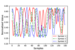
(a) The first three symbols.

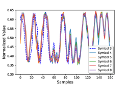
(b) The last six symbols.

Figure 2: The in-phase ZigBee signals of eight preprocessed preamble symbols.

Thus, each preamble symbol-signal $\mathbf{s}_{k}$ can be represented as

$$\mathbf{s}_{k}=RFF_{k}(\mathbf{x}_{0}),\quad k\in\left\{1,2,\cdots,8\right\},$$ (12)

where $\mathbf{\mathbf{x}_{0}}$ denotes the identical symbol 0x0 in the preamble, and $RFF_{k}(\cdot)$ denotes the RFF function on the k-th symbol. Since $\mathbf{s}_{1}\neq\mathbf{s}_{2}\neq\mathbf{s}_{3}$ and $\mathbf{s}_{3}\approx\mathbf{s}_{4}\approx\cdots\approx\mathbf{s}_{8}$, it is self-evident that:

$$RFF_{1}(\cdot)\neq RFF_{2}(\cdot)\neq RFF_{3}(\cdot),$$ (13)

$$RFF_{3}(\cdot)\approx RFF_{4}(\cdot)\approx\cdots\approx RFF_{8}(\cdot).$$ (14)

Therefore, if we study RFFs from the symbol scale, semi-steady RFFs on the first two symbols are different from steady-state RFFs on the following symbols in our target ZigBee devices.

III-B Partially Stacking

Xing et al. proposed that spread sequence in DSSS systems can be stacked to enhance SNR for increasing identification accuracy. However, in their simulation, RFF on each spread sequence must be the same. Stacking is only available for signal portions with invariable RFFs and constant data. Therefore, stacking can be applied to the steady-state portion in the preamble rather than the semi-steady portion. The partially stacking process can be expressed as

$$\begin{split}[\mathbf{s}_{1},\mathbf{s}_{2},\frac{1}{6}\sum_{i=3}^{8}\mathbf{s}_{i}]=&[RFF_{1}(\mathbf{x}_{0}),RFF_{2}(\mathbf{x}_{0}),\frac{1}{6}\sum_{i=3}^{8}RFF_{i}(\mathbf{x}_{0})]\\ =&[RFF_{1},RFF_{2},RFF_{s}](\mathbf{x}_{0})\\ =&RFF(\mathbf{x}_{0})\end{split}$$ (15)

where $RFF_{s}$ is the steady-state fingerprint, $RFF(\cdot)$ is the whole fingerprint consisted of the semi-steady fingerprint and the steady-state fingerprint.

Partially stacking is the last step of preprocessing. After partially stacking, two in-phase channels of two devices are randomly selected and demonstrated in Fig. 3. It can be seen that different devices have different RFFs, and the same device has constant RFFs in different tests. It is also evident that the RFFs in the first symbol differ the most, while the steady-state RFFs in the generated last symbols by stacking are relatively similar.

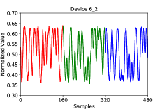
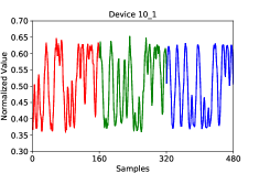
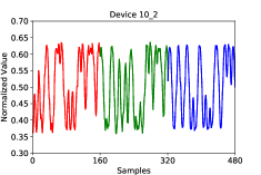
Figure 3: The in-phase channels of two partially stacked preambles for two devices.

IV Results and Discussion

IV-A Experimental System and Data Collection

Our experimental system has 27 Ti CC2530 ZigBee devices to be identified, a USRP N210 as the receiver, and a PC with MATLAB and Tensorflow for processing. ZigBee devices worked at their maximum power of 19 dBm, and they were located within one meter away from the USRP, both for enhancing the receiving SNR. In this way, the SNRs during data collection were around 30 dB. These received signals can be regarded as approximately ideal. Besides, owing to the 1 Mbps chip rate of CC2530, the sampling rate of USRP was set to 10 Msps for ten-times oversampling.

In this paper, only AWGN channels were simulated as the corruption module in Fig. 1. AWGN channels leading to SNRs changing from -10 dB to 30 dB with step 5 dB were all simulated. Hence, for each simulated SNR, the corrupted input $\mathbf{z}$ of the encoder combined with its corresponding reconstruction target $\mathbf{\hat{z}}$ and device label $\mathbf{y}$ constituted a sample $\left(\mathbf{z},\mathbf{\hat{z}},\mathbf{y}\right)$.

We had 10,944 samples, roughly 405 ones for each device. This dataset was randomly divided into 60% training data, 20% validation data, and 20% testing data. Five-fold cross-validation was carried out during the performance evaluation. The following networks were trained on the dataset including all SNRs rather than a single SNR.

IV-B Model Structure and Parameters

Our proposed DAE-based method is a general method fit for all the DL RFF approaches. Since CNN was mostly used in the existing DL RFFs as stated in Section I, we chose a CNN for performance comparison. It means the encoder and the classifier constitute a CNN, thus a CDAE comprising convolutional layers is used as the autoencoder. The structure and parameters of our model are demonstrated in Table I. The parameter selection is mainly according to our previous work [4]. As described below, different input lengths are used for comparison. When the input size is $1280\times 2$ or $960\times 2$, which means eight or six symbols, the max pooling and upsampling sizes are both $4\times 1$. When the input size decreases to $480\times 2$ or $320\times 2$, which means three or two symbols, the max pooling and upsampling sizes both decline to $2\times 1$. The reconstruction loss weight $\lambda_{1}$ and classification loss $\lambda_{2}$ are set to 1 and 10, respectively. When $\lambda_{1}=0$, our proposed CDAE model degenerates into CNN.

All our network models were trained and tested running on TensorFlow 1.12.0 with an NVIDIA GeForce GTX 1050 Ti GPU. The training was carried out by minimizing the whole loss function in (11) using an Adam solver with a batch size of 64. In addition, dropout of 0.5 and L2 regularization of 0.001 on the dense layer were used to prevent overfitting. The initial learning rate was set to 0.001. The training was repeated until the validation accuracy didn’t improve within ten epochs. Then the best validation parameters were stored for performance evaluation.

TABLE I: The layers and activation functions of the proposed CDAE model.

Network	Layer	Dimension	Activation
Input	Input	1280 (or 480) $\times$ 2	-
Encoder	Convolution	128 $\times$ (10 $\times$ 1)	ReLU
	Max Pooling	4 (or 2) $\times$ 1	-
	Convolution	128 $\times$ (3 $\times$ 2)	ReLU
	Max Pooling	4 (or 2) $\times$ 1	-
Decoder	Convolution	128 $\times$ (3 $\times$ 2)	ReLU
	UpSampling	4 (or 2) $\times$ 1	-
	Convolution	128 $\times$ (10 $\times$ 1)	ReLU
	UpSampling	4 (or 2) $\times$ 1	-
	Convolution	1 $\times$ (3 $\times$ 1)	Sigmoid
Classifier	Flatten	-	-
	Dense	1024	ReLU
	Dropout (0.5)	-	-
	Dense	27	Softmax

IV-C CNN vs. CDAE and Semi-steady RFF vs. Steady-state RFF

TABLE II: The identification rates using different networks and inputs.

SNR (dB)	CNN_2 (%)	CDAE_2 (%)	CNN_6 (%)	CDAE_6 (%)	SCNN_6 (%)	SCDAE_6 (%)	CNN_8 (%)	CDAE_8 (%)
-10	27.3	28.7	12.4	14.4	15.4	17.2	23.3	23.6
-5	50.7	52.0	24.8	26.9	31.0	35.9	43.5	47.3
0	63.4	66.1	32.5	34.0	33.5	42.7	52.6	58.3
5	81.9	84.3	48.1	53.6	49.2	58.3	77.3	82.0
10	90.7	91.4	74.8	80.4	72.1	81.1	90.7	94.6
15	94.6	95.5	90.9	91.7	83.5	93.0	96.8	98.2
20	96.8	97.1	94.5	94.9	87.3	96.7	98.1	99.4
25	96.4	96.2	96.5	97.2	90.3	98.2	97.4	99.6
30	96.9	97.7	97.4	98.4	92.6	98.5	98.0	99.8

As shown in Table II, we conducted experiments both for CNNs and CDAEs using different signal portions as inputs. Obviously, our proposed CDAE models achieve better performance at all scenarios compared to CNNs. The main performance improvement occurs in the region of [-5,10] dB.

Two-symbol semi-steady portions are fed into CNN_2 and CDAE_2 to extract the semi-steady RFF. It can be seen that the semi-steady RFF performs the best at low SNRs from -10 dB to 5 dB compared to all other inputs. The semi-steady RFF is relatively robust to AWGN channels.

The inputs of CNN_6 and CDAE_6 are six-symbol steady-state portions. Compared to CNN_2 and CDAE_2, they only behave better at very high SNRs, which means that the steady-state RFF has more fine-grained features. However, by stacking these six symbols, SCDAE_6 outperforms CDAE_6 at all SNRs, while SCNN_6 is worse than CNN_6 when SNR is not lower than 0 dB. It can be seen that CDAE can recover these fine-grained features from stacking as opposed to CNN. Hence, only stacking with appropriate processing can improve the identification rate. In a word, the semi-steady RFF contributes more than the steady-state RFF in ZigBee device identification.

Besides, we aim to evaluate the performance by using these two RFFs simultaneously. Therefore, the whole preamble is sent into CNN_8 and CAE_8 for identification, which has been employed in [7]. In this way, the identification accuracy improves at high SNRs ($\geq 10dB$), while its performance at low SNRs is still a bit poor in contrast to using the semi-steady RFF only.

IV-D Partially Stacking and Final Performance

TABLE III: Accuracies, precisions, recalls and their 95% confidence intervals for partially stacking-based CNN and CDAE models.

	PSCNN			PSCDAE
SNR (dB)	Accuracy (%)	Precision (%)	Recall (%)	Accuracy (%)	Precision (%)	Recall (%)
-10	$36.3\pm 2.1$	$34.7\pm 3.0$	$34.7\pm 2.0$	38.7$\pm$0.6	$39.4\pm 0.5$	$37.0\pm 0.7$
-5	$59.4\pm 2.0$	$61.2\pm 2.2$	$59.0\pm 2.3$	63.4$\pm$1.3	$65.7\pm 1.3$	$63.0\pm 1.1$
0	$71.5\pm 1.9$	$72.1\pm 2.0$	$70.5\pm 2.3$	76.1$\pm$1.8	$78.0\pm 1.8$	$76.3\pm 2.0$
5	$86.3\pm 2.3$	$87.8\pm 2.1$	$85.8\pm 3.0$	91.3$\pm$0.9	$92.4\pm 1.0$	$91.2\pm 1.0$
10	$95.7\pm 1.9$	$96.5\pm 1.8$	$95.6\pm 2.6$	97.5$\pm$0.5	$97.9\pm 0.5$	$97.7\pm 0.5$
15	$97.0\pm 1.1$	$97.3\pm 0.8$	$96.4\pm 1.1$	98.9$\pm$0.6	$99.2\pm 0.4$	$99.0\pm 0.6$
20	$98.6\pm 0.9$	$98.8\pm 0.6$	$98.3\pm 1.0$	99.7$\pm$0.3	$99.7\pm 0.3$	$99.7\pm 0.3$
25	$98.7\pm 0.9$	$98.5\pm 0.6$	$98.0\pm 0.9$	99.1$\pm$0.5	$99.4\pm 0.4$	$99.3\pm 0.5$
30	$99.0\pm 0.9$	$98.7\pm 0.9$	$98.5\pm 1.1$	99.0$\pm$0.5	$99.3\pm 0.4$	$99.2\pm 0.4$

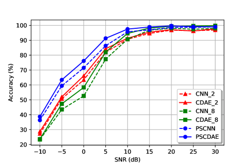
Figure 4: Performance comparison of CDAE and CNN by combining semi-steady and steady-state RFFs differently.

Since stacking with CDAE (SCDAE_6) works better than CDAE without stacking (CDAE_6), it is reasonable to imagine that PSCDAE can further improve the identification accuracy. The identification accuracies, precisions, recalls and their 95% confidence intervals of PSCDAE and Partially Stacking-based CNN (PSCNN) are manifested in Table III.

Besides, for easy comparison with SCDAE_2 and SCDAE_8 which behave the best in different SNR regions in Table II, the classification accuracies of six approaches at all SNRs are illustrated in Fig. 4. The dash lines represent CNN-based methods, and the solid lines represent CDAE-based methods. Besides, lines with the same marker have the same input. It is apparent that CDAE-based methods behave better than corresponding CNN-based methods, especially at SNRs from -5 dB to 10 dB. Furthermore, PSCDAE has the best accuracy at almost all SNRs, which demonstrates that it can combine semi-steady and steady-state RFFs effectively. It is also noticeable that PSCDAE is a bit worse than CDAE_8 by $5\permil$ and $8\permil$ at 25 dB and 30 dB, respectively. This is owing to the information loss during stacking. As stated in (14), the steady-state RFFs in the six preamble symbols are almost equal, but some different fine-grained features still exist. These fine-grained features can be extracted by CDAE_8 at high SNRs for identification. While as SNR goes down, these features will be gradually covered by noise.

By comparison with CNN_8 which is used in [7], PSCDAE can respectively improve the identification accuracy by 15.4%, 19.9%, 23.5%, 14.0%, 6.8%, 2.1%, 1.6%, 1.7%, 1.0% at SNRs from -10 dB to 30 dB with step 5 dB. Besides, according to Table III, it is also crystal-clear that the 95% confidence intervals for PSCDAE are almost only half of that for PSCNN. This is to say, models trained by PSCDAE are more precise than those trained by PSCNN. In other words, performance fluctuations of PSCDAE are smaller. Furthermore, it can be seen that the accuracy of PSCDAE first increases dramatically and then slightly goes down, it reaches the top when SNR is equal to 20 dB. This is because, at high SNRs, the gain introduced by the autoencoder is gradually lost. Due to the existing reconstruction loss in the optimization objective, those fine-grained features that are useful for classification while adverse to reconstruction cannot be learned by PSCDAE.

V Conclusions

This paper has demonstrated a universal DAE-based framework for DL RFF approaches. A partially stacking technique has also been proposed to leverage both the semi-steady and steady-state RFFs efficiently for identifying ZigBee devices. A two-layer CNN and the corresponding CDAE model have been used to show the superiority of our proposed scheme. We have conducted various experiments on our testbed which includes a USRP as the receiver and 27 CC2530 nodes as targets. Experimental results demonstrate that our proposed PSCDAE outperforms the traditional CNN in [7] by 14% to 23.5% at low SNRs (-10 dB to 5 dB) under AWGN channels in terms of identification accuracy. At high SNRs, it can also slightly improve performance. Besides, the models trained by PSCDAE are much more robust than those trained by CNN. In future work, we will focus on studying multipath channels as the corruption module as well as using images derived from transforms as the input.

Acknowlegment

This work was supported in part by the National Natural Science Foundation of China under Grant 61571110, 61602113, 61601114, 61801115, Purple Mountain Laboratories (PML) and Campus France.

References

- [1] G. Li, C. Sun, J. Zhang, E. Jorswieck, B. Xiao, and A. Hu, “Physical layer key generation in 5G and beyond wireless communications: Challenges and opportunities,” Entropy, vol. 21, no. 5, p. 497, 2019.
- [2] D. Bastos, M. Shackleton, and F. El-Moussa, “Internet of things: A survey of technologies and security risks in smart home and city environments,” in Proc. Living in the IoT: Cybersesecur. IoT-2018, London, UK, Mar. 2018, pp. 1–7.
- [3] C. Morin, L. Cardoso, J. Hoydis, J.-M. Gorce, and T. Vial, “Transmitter classification with supervised deep learning,” in Proc. EAI Int. Conf. Cogn. Radio Oriented Wireless Netw. (CROWNCOM), Poznan, Poland, Jun. 2019, pp. 1–14.
- [4] J. Yu, A. Hu, G. Li, and L. Peng, “A robust RF fingerprinting approach using multi-sampling convolutional neural network,” IEEE Internet Things J., pp. 1–1, 2019.
- [5] S. S. Hanna and D. Cabric, “Deep learning based transmitter identification using power amplifier nonlinearity,” in Proc. IEEE Int. Conf. Comput. Netw. Commun. (ICNC), Honolulu, HI, USA, Apr. 2019, pp. 674–680.
- [6] P. Robyns, E. Marin, W. Lamotte, P. Quax, D. Singelée, and B. Preneel, “Physical-layer fingerprinting of LoRa devices using supervised and zero-shot learning,” in Proc. ACM Conf. Secur. Privacy Wireless Mobile Netw. (WiSec), Boston, MA, USA, Jul. 2017, pp. 58–63.
- [7] K. Merchant, S. Revay, G. Stantchev, and B. Nousain, “Deep learning for RF device fingerprinting in cognitive communication networks,” IEEE J. Sel. Topics Signal Process., vol. 12, no. 1, pp. 160–167, Feb. 2018.
- [8] Q. Wu, C. Feres, D. Kuzmenko, D. Zhi, Z. Yu, X. Liu et al., “Deep learning based RF fingerprinting for device identification and wireless security,” Electron. Lett., vol. 54, no. 24, pp. 1405–1407, Nov. 2018.
- [9] G. Baldini, C. Gentile, R. Giuliani, and G. Steri, “Comparison of techniques for radiometric identification based on deep convolutional neural networks,” Electron. Lett., vol. 55, no. 2, pp. 90–92, Jan. 2019.
- [10] G. Baldini, R. Giuliani, and F. Dimc, “Physical layer authentication of Internet of Things wireless devices using convolutional neural networks and recurrence plots,” Internet Technol. Lett., vol. 2, no. 2, p. e81, Mar./Apr. 2019.
- [11] K. Youssef, L. Bouchard, K. Haigh, J. Silovsky, B. Thapa, and C. Vander Valk, “Machine learning approach to RF transmitter identification,” IEEE J. Radio Freq. Identification, vol. 2, no. 4, pp. 197–205, Nov. 2018.
- [12] Y. Pan, S. Yang, H. Peng, T. Li, and W. Wang, “Specific emitter identification based on deep residual networks,” IEEE Access, pp. 54 425–54 434, Apr. 2019.
- [13] H. Huang, J. Yang, H. Huang, Y. Song, and G. Gui, “Deep learning for super-resolution channel estimation and DOA estimation based massive mimo system,” IEEE Trans. Veh. Technol., vol. 67, no. 9, pp. 8549–8560, Sep. 2018.
- [14] Y. Xing, A. Hu, J. Zhang, L. Peng, and G. Li, “On radio frequency fingerprint identification for DSSS systems in low SNR scenarios,” IEEE Commun. Lett., vol. 22, no. 11, pp. 2326–2329, Nov. 2018.
- [15] Y. Bengio, P. Lamblin, D. Popovici, and H. Larochelle, “Greedy layer-wise training of deep networks,” in Proc. Advances Neural Inform. Process. Syst. (NIPS), Vancouver, B.C., Canada, Dec. 2007, pp. 153–160.
- [16] P. Vincent, H. Larochelle, Y. Bengio, and P.-A. Manzagol, “Extracting and composing robust features with denoising autoencoders,” in Proc. ACM 25th Int. Conf. Mach. Learn. (ICML), Helsinki, Finland, Jun. 2008, pp. 1096–1103.
- [17] L. Peng, A. Hu, J. Zhang, Y. Jiang, J. Yu, and Y. Yan, “Design of a hybrid RF fingerprint extraction and device classification scheme,” IEEE Internet Things J., vol. 6, no. 1, pp. 349–360, Feb. 2019.