Spectral Lag for a Radiating Jet Shell with a High Energy Cut-off Radiation Spectrum

Abstract

Recent research shows that the spectral lag is closely related to the spectral evolution in GRBs. In this paper, we study the spectral lag for a radiating jet shell with a high-energy cut-off radiation spectrum. For the jet shell with a cut-off power-law spectrum, the spectral lag monotonically increases with the photon energy and levels off at a certain photon energy. It is the same for the jet shell with a Band cut-off spectrum (Bandcut). However, a turn-over from the positive lags to negative lags appears in the high-energy range for the jet shell with Bandcut, which is very similar to that observed in GRB 160625B. The dependence of the spectral lags on the spectral shape/evolution are studied in details. In addition, the spectral lag behavior observed in GRB 160625B is naturally reproduced based on our theoretical outcome.

1 Introduction

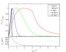
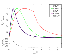
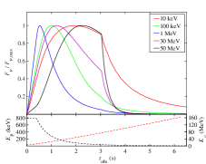
Figure 1: The simulated light curves (upper sub-figure) and $E_{\rm ch}$ or $E_{\rm p}$ ($E_{\rm c}$) evolution (lower sub-figure) for the physical model (see Section 2.1) with CPL (left panel), Band (middle panel), and Bandcut (right panel) radiating photon spectrum, respectively. The red, green, blue, purple, and, black lines are corresponding to the light curves observed at $E_{\rm obs}=$10 keV, 100 keV, 1 MeV, 30 MeV, and 50 MeV, respectively.

Gamma-ray bursts (GRBs) are the most energetic electromagnetic explosions in the Universe. The temporal structure of prompt gamma-ray emission exhibits diverse morphologies (Fishman & Meegan, 1995), which can vary from a single smooth large pulse to an extremely complex light curve with many erratic overlapping pulses (see fig. 1 in Pe’er, 2015). The radiation spectrum evolves uniformly within a GRB’s pulse, which suggests that pulses are fundamental units of GRB radiation (Lu et al., 2018). Thus, the observed temporal and spectral behaviors of GRB’s pulses may provide an interesting clue to understand the nature of GRBs.

The spectral lag, referring to the difference of the arrival time for different energy photons, is a common feature of pulses in GRBs (Norris et al., 1986; Cheng et al., 1995; Band, 1997; Norris et al., 2000; Chen et al., 2005; Peng et al., 2007). Early in the BATSE era, it was found that most of the GRBs pulses are dominated by the positive lags (i.e., the soft photons lag behind the hard photons), and a small fraction of pulses show negative lags (e.g., Yi et al. 2006). Generally, the bursts with long-wide pulses tend to have long lags and soft hardness (Norris et al., 2000, 2001b, 2005; Daigne & Mochkovitch, 2003). The extensive analyses based on the GRBs observations by BATSE revealed that, the lag features between the bursts divided by 2s-$T_{90}$-duration time (Kouveliotou et al., 1993) show distinct discrepancies (Band, 1997; Norris et al., 2000, 2001a; Yi et al., 2006), which has been suggested as a new classification scheme for GRBs (Norris & Bonnell, 2006; Gehrels et al., 2006; McBreen et al., 2008; Zhang et al., 2009). Besides, an inverse correlation between lag and the peak luminosity was found by Norris et al. (2000) based on six redshift-known bursts, which is further confirmed by GRBs observed by BAT onboard the Swift satellite (Ukwatta et al., 2010, 2012). This correlation is proposed to be a GRBs distance indicator to probe cosmology (Norris, 2004; Schaefer, 2003, 2007; Gao et al., 2012).

Despite of decades of research, the true physical origin of the spectral lag is still inconclusive. It was suggested that the curvature effect of the spherical fireball is a plausible explanation for the spectral lag (e.g., Ioka & Nakamura 2001; Shen et al. 2005; Lu et al. 2006; Shenoy et al. 2013). In this scenario, the emission from the spherical shells at progressively higher latitudes with respect to the observer’s line of sight is progressively delayed due to the weaker Doppler-boosting effect, such that the light curves of low energy radiation would be delayed and peak at later times. But the main difficulty of curvature effect model is that the flux levels at different energy bands are particularly lower than the observed (Zhang et al., 2009). Uhm & Zhang (2016b) pointed out that there would be essentially unnoticeable spectral lags given rise from the high-latitude emission, as well as the properties of light curves are not in accord with the observations. Instead, they proposed a physical model invoking a spherical shell rapidly expands in the bulk-accelerating region, which is suggested to be more reasonable to account for the spectral lags (Uhm & Zhang, 2016b; Wei et al., 2017; Shao et al., 2017; Lu et al., 2018; Uhm et al., 2018). In the framework of the internal shock model, Bošnjak & Daigne (2014) have made the thorough study of spectral evolution and investigated the spectral lags.

Recently, Lu et al. (2018) reveals that the spectral lags are strongly related to the spectral evolution in GRB’s pulses, stimulating us the motivation to explore the nature of spectral lag. The previous works mainly focus on a radiating jet shell with a Band radiation spectrum. However, there are a sample of GRBs of which the radiation spectrum deviates from the Band spectrum, e.g., cut-off power-law (e.g., GRB 170817A, Zhang et al., 2018) or Band cut-off radiation spectrum (e.g., GRB 160625B, Lin et al., 2018). Thus, we would like to study the spectral lag behavior in the case that the jet shell radiates with a high-energy cut-off spectrum based on the theory in Uhm & Zhang (2016b). The contents of our paper are arranged as follows. In Section 2, we describe the details of the physical model constructed in Uhm & Zhang (2016b) and explore the spectral lag behavior for GRBs with a cut-off radiation spectrum. We also employ a phenomenological model to explore the dependence of the spectral lag behavior on the spectral shape/evolution. In Section 3, we discuss the spectral lags in GRB 160625B. Our conclusions are presented in Section 4. The flat $\Lambda$CDM cosmology with $\Omega_{\rm M}=0.27$ and $H_{0}=71$ km/s/Mpc is adopted throughout this work.

2 Spectral Lag for a Radiating Jet Shell with a Cut-off Radiation Spectrum

2.1 Physical Model

To investigate the spectral lag of GRBs’ pulses, we adopt the physical model constructed in Uhm & Zhang (2016b). The physical model involves a relativistic jet shell, which undergoes a rapid bulk acceleration and continuously emits photons with an isotropic distribution in its co-moving frame. Same as Uhm & Zhang (2016b), the radiation of the jet shell in our model is turned on at the radius $r_{\rm{on}}=10^{14}$ cm and turned off at $r_{\rm off}=3\times 10^{16}$ cm, where the line-of-sight emission finally ceases. The value of $r_{\rm{on}}$ and $r_{\rm off}$ are fixed in our numerical calculations. The synchrotron radiation is taken as the main emission mechanism and the shape of the radiation spectrum in the shell co-moving frame is described in the form of (Uhm & Zhang, 2015)

$$P^{\prime}(E)=nP^{\prime}_{e}H(x)\;\,{\rm with}\;\,{x=E^{\prime}/{E^{\prime}_{\rm{ch}}}}$$ (1)

where $n$ represents the number density of radiating electrons, $H$ is the normalized photon spectrum, and $P^{\prime}_{e}$ ($E^{\prime}_{\rm{ch}}$) is the radiation spectral power (characteristic photon energy) of an emitting electron with Lorentz factor $\gamma_{\rm{ch}}$, i.e.,

$$P^{\prime}_{e}=\frac{3\sqrt{3}}{32}\frac{m_{e}c^{2}\sigma_{T}B}{q_{e}},$$ (2)

$$E^{\prime}_{\rm{ch}}=h\nu^{\prime}_{\rm{ch}}=\frac{3}{16}\frac{hq_{e}B}{m_{e}c}\gamma_{\rm{ch}}^{2}.$$ (3)

Here, $m_{\rm e}$ ($q_{\rm e}$) is the mass (charge) of electrons, $c$ is the speed of light, $\sigma_{\rm T}$ represents the Thompson cross section, $h$ is the Planck constant, and $B$ is the strength of magnetic field in the co-moving frame. The relativistic electrons are speculated to be uniformly distributed in the shell co-moving frame and isotropically collected into the fluid with a constant injection rate $R_{\rm inj}=dn/dt^{\prime}$. Observationally, the sub-MeV photon spectrum of a typical GRBs can be well fitted by a smoothly joint broken power-law function (Band function; Band et al. 1993), with a cut-off rarely observed in the high-energy bands. In this work, we study the spectral lag behavior in the following three spectral shapes:
(I) the cut-off power-law radiation spectrum (CPL)

$$H(x)=x^{\alpha}e^{-x},$$ (4)

(II) the Band radiation spectrum (Band)

$$H(x)=\left\{\begin{array}[]{lcl}x^{\alpha}e^{-x},&&x<(\alpha-\beta),\\ (\alpha-\beta)^{\alpha-\beta}e^{\beta-\alpha}x^{\beta},&&x\geq(\alpha-\beta),\\ \end{array}\right.$$ (5)

(III) the Band radiation spectrum with a high-energy cut-off (Bandcut)

$$H(x)=H^{\rm Band}(x){\rm exp}{\left(\frac{-xE^{\prime}_{\rm ch}}{E^{\prime}_{\rm c}}\right)},$$ (6)

where $\alpha$ and $\beta$ are the spectral indices. $E^{\prime}_{\rm c}(\gg E^{\prime}_{\rm ch})$ represents the high-energy cut-off behavior, which may be caused by the absorption of two-photon pair production (e.g., Krolik & Pier, 1991; Fenimore et al., 1993; Woods & Loeb, 1995; Baring & Harding, 1997; Ackermann et al., 2011, 2013; Tang et al., 2015). For the above three kinds of radiation spectrum, the peak energy of $\nu F_{\nu}$ spectrum is $E_{\rm p}=(2+\alpha)E_{\rm ch}$. It is worthy to point out that $E_{\rm p}=(2+\alpha)E_{\rm ch}$ is only applicable for Bandcut with $E^{\prime}_{\rm c}\gg E^{\prime}_{\rm ch}$, which is the cases studied in this paper.

The photons emitted in the shell co-moving frame would be Doppler-boosted with a factor of $D=1/\left[\Gamma\left(1-\beta\cos\theta\right)\right]$, where $\Gamma$ is the bulk Lorentz factor of the jet shell, $\beta=\sqrt{1-1/\Gamma^{2}}$, and $\theta$ is the latitude of the emission location relative to the observer’s line of sight. Similar to Uhm & Zhang (2016a), the evolution of $\Gamma$ and $B$ are described as

$$\Gamma(r)=\left\{{\begin{array}[]{*{20}{c}}{{\Gamma_{0}},}&{{r_{{\rm{on}}}}<r\leq{r_{0}},}\\ {{\Gamma_{0}}{{(r/{r_{0}})}^{s}},}&{r>{r_{0}},}\end{array}}\right.$$ (7)

$$B(r)=\left\{{\begin{array}[]{*{20}{c}}{{B_{0}},}&{{r_{{\rm{on}}}}<r\leq{r_{0}},}\\ {{B_{0}}{{(r/{r_{0}})}^{-b}},}&{r>{r_{0}},}\end{array}}\right.$$ (8)

where $\Gamma_{0}$ ($B_{0}$) is the normalization value at the radius $r_{0}$ of $\Gamma$ ($B$) and the power-law index $s>0$ ($b>0$) is adopted (Uhm & Zhang, 2014, 2016b). In this model, the jet is Poynting-flux-dominated and the magnetic field is dissipated via reconnection of oppositely oriented field lines as the jet propagates outward. This is different from that in the particle-in-cell (PIC) simulations of internal shock model, in which the simulations of shocks indicate that the Weibel instability-induced filaments merge and cause the magnetic field to gradually decay (e.g., Chang et al., 2008; Keshet et al., 2009; Silva et al., 2003; Medvedev et al., 2005). The PIC simulation of Chang et al. (2008) indicates that the magnetic field decays as a power law of time in the downstream co-moving frame (see also, e.g., Lemoine et al., 2013; Zhao et al., 2014), and the longer PIC simulation by Keshet et al. (2009) seems to result in an exponential decay with time. The observed time $t_{\rm{obs}}$ of a photon emitted from the radius $r$ and latitude $\theta$ can be described as

$$t_{\rm{obs}}(r,\theta)=\left[\int_{{r_{{\rm{on}}}}}^{r}{\frac{{1-\beta}}{{\beta c}}dl}+\frac{r(1-\rm cos\theta)}{c}\right](1+z).$$ (9)

The observed flux density $F_{\nu,\rm{obs}}$ is calculated with

$$F_{\nu,\rm{obs}}=\int_{\rm(EATS)}{\frac{nP^{\prime}_{\rm e}D^{3}H(x)(1+z)}{4\pi D^{2}_{\rm L}(z)}d\Omega}$$ (10)

where EATS is the equal-arrival time surface corresponding to the same observer time $t_{\rm obs}$ and $D_{\rm L}$ is the luminosity distance at the redshift $z$.

The spectral lags are estimated based on the discrepancy of light curves’ peak time. In this section, we adopt the following model parameters in our numerical calculations (Uhm & Zhang, 2016b): $\alpha=-0.8$, $\beta=-2.3$, $\gamma_{\rm ch}=8\times 10^{4}$, $\Gamma_{0}=300$, $B_{0}=30$ G, $r_{0}=10^{15}$ cm, $s=0.35$, $b=1.25$, $R_{\rm{inj}}=10^{47}~{}{\rm s}^{-1}$, and $z=1.406$ (GRB 160625B; Xu et al. 2016). With above parameters, the observed characteristic photon energy in the spectrum is $E_{\rm ch}\simeq 653$ keV at $t_{\rm obs}=0$ s and the shell curvature effect shaping the light curves occurs at $t_{\rm obs}\gtrsim 3$ s. For the high-energy cut-off behavior in the case with Bandcut, we assume the cut-off energy in the co-moving frame is $E^{\prime}_{\rm c}=20{\rm MeV}/2\Gamma_{\rm off}$ ( $\Gamma_{\rm off}=\Gamma_{0}r_{\rm off}^{s}/r_{0}^{s}\sim 990$) and remains constant during the expansion of the jet shell. Then, the observed high-energy cut-off $E_{\rm c}$ is $\simeq 6$ MeV at $t_{\rm obs}=0$ s and increases in the case with $s>0$, which is studied in this section.

2.2 High-energy Spectral Lag in the Physical Model

We numerically calculate the light curves for the physical model in Section 2.1. The results are shown in Figure 1, where the light curves are normalized with its peak flux $F_{\nu,\rm max}$ and the red, green, blue, purple, and black lines are corresponding to the observed photon energy of $E_{\rm obs}=$10 keV, 100 keV, 1 MeV, 30 MeV, and 50 MeV, respectively. The cases with CPL, Band, and Bandcut are studied in the left, middle, and right panels, respectively. In each panel, the upper part plots the light curves at different $E_{\rm obs}$ and the lower part shows the evolution of $E_{\rm p}$ (black dashed line) and $E_{\rm c}$ (red dashed line) if it exists. As one can find from Figure 1, the spectral lags are distinctly visible for the hard photons relative to the soft photons (e.g., 10 keV). Moreover, the spectral lags for photons above $E_{\rm c}$ are dramatically different for the case with Band and that with Bandcut by comparing the purple ($E_{\rm obs}=30$ MeV) or black ($E_{\rm obs}=50$ MeV) lines. Here, both the purple and black lines overlap the blue line ($E_{\rm obs}=1$ MeV) in the Band case but lag behind the blue line in the Bandcut case. Then, we study the relation of peak time $t_{\rm p}$ and $E_{\rm obs}$ in the left panel of Figure 2, where the cases with CPL, Band, and Bandcut are shown with “$\circ$”, “$\Box$”, and “$\times$” symbols, respectively. In this panel, we also plot the observed relation $t_{\rm p}\propto E_{\rm obs}^{-0.25}$ (Band, 1997; Liang et al., 2006) with dashed line for a comparison. One can find that our $t_{\rm p}-E_{\rm obs}$ relations at higher $E_{\rm obs}$ deviate from the relation of $t_{\rm p}\propto E_{\rm obs}^{-0.25}$. For the0 cases with CPL and Band, the $t_{\rm p}$ levels off for high $E_{\rm obs}$. For the Bandcut case, $t_{\rm p}$ also levels off at $E_{\rm obs}\sim 1$ MeV but begins to rise at $E_{\rm obs}\sim 10$ MeV. In the right panel of Figure 2, we show the spectral lags $\tau$ of high-energy photons with respect to the low-energy photons (e.g., $E_{\rm obs}=10$ keV), i.e.,

$$\tau=t_{\rm p}(E_{\rm obs}=10\,{\rm keV})-t_{\rm p}(E_{\rm obs}).$$ (11)

Here, the cases with CPL, Band, and Bandcut are also shown with “$\circ$”, “$\Box$”, and “$\times$” symbols, respectively. It can be found that the spectral lag $\tau$ increases with $E_{\rm obs}$ and levels off at $E_{\rm obs}\gtrsim E_{\rm s}\sim 0.8\,\rm MeV$ for all cases. However, a turn-over at $E_{\rm obs}\gtrsim E_{\rm t}\sim 10$ MeV appears in the case with Bandcut but does not present in the cases with CPL or Band. This is the main finding in this work and has been observed in GRB 160625B for the first time (Wei et al., 2017). We will further study this behavior in Section 2.3.

2.3 Detail Study on the High-energy Spectral Lags

Lu et al. (2018) systematically studies the relation between the spectral lags and spectral evolution based on a sample of Fermi GRB pulses. It is shown that the spectral lags are closely related to the spectral evolution. In Section 2.2, a pattern of positive lags is found. In addition, a high-energy turn-over in the $t_{\rm p}-E_{\rm obs}$ and $\tau-E_{\rm obs}$ relations is presented in the case with Bandcut, which is not studied in previous works. Then, we would like to present a detailed study on the relationship of the spectral lags and the spectral evolution in this section, especially for the case with a cut-off radiation spectrum. To be more generic for our studies, we employ the phenomenological model in Lu et al. (2018) by giving the observed patterns of light curves and spectral evolution. The reasons to adopt the phenomenological model are shown as follows. (1) The calculations based on the physical model is too time-consuming. (2) The phenomenological model can describe the GRB phenomena without specifying any physical models. Then, the results obtained based on the phenomenological model is applicable for a number of GRB emission models, e.g., the internal shock model (Rees & Mészáros, 1994), the photosphere emission model (Goodman, 1986; Paczynski, 1986; Thompson, 1994; Mészáros, & Rees, 2000), the internal-collision induced magnetic reconnection and turbulence (Zhang & Yan, 2011; Deng et al., 2016), and the external reverse shock model (e.g., Shao & Dai, 2005; Kobayashi et al., 2007; Fraija, 2015; Fraija et al., 2016). In the phenomenological model, the observed flux density of a GRB pulse is modeled with

$$F_{\nu}(t_{\rm obs},E_{\rm obs})=I_{\nu}(t_{\rm obs})H(E_{\rm obs}/E_{\rm ch})/E_{\rm ch},$$ (12)

where $I_{\nu}(t_{\rm obs})$ is the intensity identified with an empirical pulse model (Kocevski et al., 2003; Lu et al., 2018)

$$I_{\nu}(t_{\rm obs})=I_{\rm p,f}\left(\frac{t_{\rm obs}-t_{0}}{t_{\rm p,f}-t_{0}}\right)^{\mathcal{R}}\left[\frac{\mathcal{D}}{\mathcal{D}+\mathcal{R}}+\frac{\mathcal{R}}{\mathcal{D}+\mathcal{R}}\left(\frac{t_{\rm obs}-t_{0}}{t_{\rm p,f}-t_{0}}\right)^{(\mathcal{R}+1)}\right]^{-\frac{\mathcal{R}+\mathcal{D}}{\mathcal{R}+1}}.$$ (13)

Here, $t_{0}$ corresponds to the zero time of pulse, and $\mathcal{R}$ and $\mathcal{D}$ are the power-law indices before and after the time ($t_{\rm p,f}$) of the peak flux ($I_{\rm p,f}$) in full-wave band. For the temporal evolution of $E_{\rm p}=(2+\alpha)E_{\rm ch}$, we adopt the hard-to-soft mode (Lu et al., 2018), i.e.,

$$E_{\rm p}(t_{\rm obs})=E_{\rm p,0}\left(1+\frac{t_{\rm obs}-t_{0}}{t_{\rm c}}\right)^{-k_{\rm p}}\;\text{ with }\;k_{\rm p}>0,$$ (14)

where $t_{\rm c}$ is the characteristic timescale of the $E_{\rm p}$’s evolution. In observations, the observed high-energy cut-off $E_{\rm c}$ may also evolve with time, e.g., the value of $E_{\rm c}$ in the second sub-burst of GRB 160625B increases with $t_{\rm obs}$ (Lin et al., 2018). Then, the temporal evolution of $E_{\rm c}$ in the Bandcut case is set to be

$$E_{\rm c}(t_{\rm obs})=E_{\rm c,0}\left(1+\frac{t_{\rm obs}-t_{0}}{t_{\rm c}}\right)^{k_{\rm c}}\;\text{ with }\;k_{\rm c}>0.$$ (15)

In this section, we adopt the following model parameters in our numerical calculations: $I_{\rm p,f}=1$, $\mathcal{R}=1$, $\mathcal{D}=3$, $t_{0}=0$ s, $t_{\rm p,f}=5$ s, $E_{\rm p,0}=1$ MeV, $E_{\rm c,0}=20$ MeV, $k_{\rm p}=1$, and $k_{\rm c}=0.5$, respectively. With these parameters, the rise timescale of the pulse in bolometric luminosity is around $3.5$ s and thus the value of $t_{c}=3.5$ s is adopted.

With above phenomenological descriptions, we explore the spectral lag behavior for the cases with a high-energy cut-off radiation spectrum, i.e., CPL and Bandcut. The synthetic light curves (upper part) as well as the spectral evolution (lower part) are shown in the left (CPL case) and middle (Bandcut case) panels of Figure 3, where the light curves observed at the photon energy $E_{\rm obs}=10$ keV, 100 keV, 1 MeV, 30 MeV, and 50 MeV are plotted with red, green, blue, purple, and black lines, respectively. For the lower part of middle panel, the evolution of $E_{\rm p}$ ($E_{\rm c}$) is drawn with dashed black (red) line. In addition, the peak time of each light curve is denoted by the same color vertical dashed line. According to these light curves, one can find the very different spectral lag behaviors of $E_{\rm obs}>E_{\rm c}$ (e.g., purple or black line) for the case with CPL and that with Bandcut. This result is consistent with that found in Section 2.2. The right panel of Figure 3 displays the relations of $\tau-E_{\rm obs}$, where “$\circ$” and “$\times$” symbols denote the results from the cases with CPL and that with Bandcut, respectively. The relations of $\tau-E_{\rm obs}$ in this panel are also consistent with those obtained in Section 2.2. Especially, a turn-over of $\tau-E_{\rm obs}$ relation in the high-energy channels also appears in the Bandcut case, which is what we mainly expect. These results suggest that the spectral lag revealed by the phenomenological model is consistent with that estimated based on the physical model.

Based on the $\tau-E_{\rm obs}$ relations in the right panels of Figures 2 and 3, we formulate the spectral lag behavior as follows,

$$\tau=\begin{cases}\tau_{0}\frac{E_{\rm obs}^{k_{\rm s}}-E^{k_{\rm s}}_{\rm m}}{E^{k_{\rm s}}_{\rm s}-E^{k_{\rm s}}_{\rm m}},&E_{\rm obs}\leqslant E_{\rm s}\\ \tau_{0}\left[1+\left(\frac{E_{\rm obs}}{E_{\rm t}}\right)^{k_{\rm t}\omega}\right]^{\frac{1}{\omega}},&E_{\rm obs}>E_{\rm s}\end{cases}$$ (16)

where $\tau_{0}$ is the spectral lag at $E_{\rm obs}=E_{\rm s}$, $E_{\rm m}$ is the specified lowest energy (e.g., 10 keV), $k_{\rm s}$ ($k_{\rm t}$) is the power-law index for the energy range $E_{\rm obs}<E_{\rm s}$ ($E_{\rm obs}>E_{\rm t}$), and $\omega$ describes the sharpness around the break $E_{\rm t}$ (actually $\omega=1$ is adopted in this work). Equation (16) is applicable for the case with CPL or Band by setting $E_{\rm t}$ significantly high (e.g., $E_{\rm t}\rightarrow\infty$). The dashed lines in right panels of Figures 2 and 3 are the fitting results based on Equation (16), where the cases with CPL, Band, and Bandcut are shown with the blue, green, and red color. It can be found that Equation (16) well describes the relations of $\tau-E_{\rm obs}$.

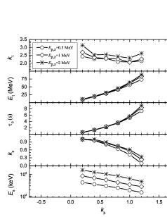
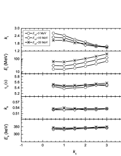
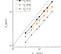
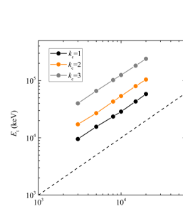
Figure 4: Upper panel: correlations between the spectral lag behavior and $\alpha$ (left) and/or $\beta$ (right) in the Bandcut spectrum; Middle panel: the dependence of the spectral lag behavior on the $k_{\rm p}$ for different $E_{\rm p,0}$ (left) and $k_{\rm c}$ for different $E_{\rm c,0}$ (right) ; Lower panel: the relations of $E_{\rm s}-E_{\rm p,0}$ (left) for different $k_{\rm p}$ and $E_{\rm t}-E_{\rm c,0}$ (right) for different $k_{\rm c}$, and the dashed line in each panel denotes the case of $E_{\rm s}=E_{\rm p,0}$ or $E_{\rm t}=E_{\rm c,0}$.

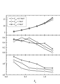
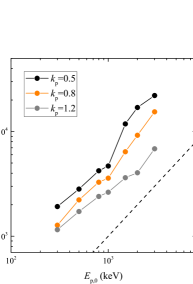
Figure 5: Upper panel: correlations between the spectral lag behavior and $\lambda$ (left) and/or $k_{\rm p}$ (right) for the case with CPL; Lower panel: the relations of $E_{\rm s}-E_{\rm p,0}$ for different $k_{\rm p}$, and the dashed line denotes the case of $E_{\rm s}=E_{\rm p,0}$.

In this part, we investigate the dependence of the spectral lag behavior on the radiation spectral shape/evolution for the case with CPL or Bandcut. We first study the case with Bandcut and the results are shown in Figure 4. Here, the upper-left (right) panel displays the relations between the spectral lag behavior (i.e., $E_{\rm s}$, $k_{\rm s}$, $\tau_{0}$, $E_{\rm t}$, and $k_{\rm t}$) and the spectral index $\alpha$ ($\beta$) by adopting $E_{\rm p,0}=1$ MeV, $k_{\rm p}=1$, $E_{\rm c,0}=20$ MeV, and $k_{\rm c}=0.5$. One can find that the value of $\tau_{0}$ and thus the spectral lag increases with $\alpha$ while decreases with $\beta$. In addition, the $\tau-E_{\rm obs}$ relation in the energy range of $E_{\rm obs}<E_{\rm s}$ becomes shallower (steeper) by increasing the value of $\alpha$ ($\beta$). However, the $k_{\rm t}$ is not related to the spectral shape. For the two characteristic photon energy in the $\tau-E_{\rm obs}$ relations, $E_{\rm s}$ decreases by increasing $\alpha$ or $\beta$, and $E_{\rm t}$ increases with $\alpha$ and decreases with $\beta$. In the middle-left (right) panel of Figure 4, we show the relations between the spectral lag behavior (i.e., $E_{\rm s}$, $k_{\rm s}$, $\tau_{0}$, $E_{\rm t}$, and $k_{\rm t}$) and the spectral evolution index $k_{\rm p}$ ($k_{\rm c}$) by setting $\alpha=-0.8$ and $\beta=-2.3$. Here, $E_{\rm p,0}=0.5$, 1, 2 MeV ($E_{\rm c,0}=5$, 10, 20 MeV) are adopted in the left (right) panel and plotted with “$\circ$”, “$\diamond$”, and “$\ast$” symbols, respectively. From these panels, one can find that the values of $E_{\rm s}$, $k_{\rm s}$, and $\tau_{0}$ are related to the value of $k_{\rm p}$ but does not depend on the $k_{\rm c}$. It reveals that the values of $E_{\rm s}$, $k_{\rm s}$, and $\tau_{0}$ are associated with the Band spectrum part of Bandcut rather than the high-energy cut-off behavior. Moreover, the $\tau-E_{\rm obs}$ relation in the energy range of $E_{\rm obs}<E_{\rm s}$ becomes shallower by increasing the value of $k_{\rm p}$. The spectral lag becomes larger by adopting high value of $k_{\rm p}$, which is consistent with the observed one (e.g., the left panel of figure 6 in Lu et al., 2018). The value of $k_{\rm p}$ and $k_{\rm c}$ also affects the turn-over behavior of the $\tau-E_{\rm obs}$ relations in the high-energy range. The higher value of $k_{\rm p}$ or $k_{\rm c}$ adopted, the higher value of $E_{\rm t}$ would be. In addition, a low value of $k_{\rm t}$ would be produced in the case with high $k_{\rm c}$. It is interesting to point out that the value of $E_{\rm p,0}$ ($E_{\rm c,0}$) only influences the value of $E_{\rm s}$ ($E_{\rm t}$). Then, we plot the relation of $E_{\rm s}-E_{\rm p,0}$ ($E_{\rm t}-E_{\rm c,0}$) in the lower-left (right) panel. One can find that $E_{\rm s}$ ($E_{\rm t}$) is proportional to $E_{\rm p,0}$ ($E_{\rm c,0}$), which is not associated to the $k_{\rm p}$ ($k_{\rm c}$). These results indicate that the spectral lag is strongly related to the spectral shape and evolution. We also investigate the dependence of the spectral lag behavior on the radiation spectral shape/evolution for the case with CPL. The results are shown in Figure 5. For the cases with CPL, the $\tau-E_{\rm obs}$ relation can be described with three parameters, i.e., $E_{\rm s}$, $k_{\rm s}$, and $\tau_{0}$ . The left and middle panels of Figures 5 show the dependence of the above three parameters on the $\alpha$ and $k_{\rm p}$, respectively. The dependences of $E_{\rm s}$, $k_{\rm s}$, and $\tau_{0}$ on the value of $\alpha$ ($k_{\rm p}$) are almost consistent with those found in the Bandcut case. In addition, the value of $E_{\rm s}$ is also proportional to the value of $E_{\rm p,0}$. This behavior is also consistent with that found in the Bandcut case.

3 Discussion: Application to GRB 160625B

The prompt $\gamma$-ray emission of GRB 160625B consists of three distinct emission episodes with a total duration of about $T_{90}=770$ s (15-350 keV; Zhang et al. 2018). The first sub-burst (episode I) that triggered the Fermi/GBM at $T_{0}$=22:40:16.28 UT on 2016 June 25 lasts approximately 0.8 s with soft radiation spectrum. At $T_{0}+188.54$ s, the Fermi/LAT detected the main sub-burst (episode II), which is an extremely bright episode with multiple peaks and a duration of about 35 s. The main sub-burst is also detected by the GBM detector. After a long quiescent stage of 339 s, the GBM was triggered again, resulting in the third sub-burst (episode III) with a duration of about 212 s. The spectroscopic observations of the absorptions lines are coincident with Mg I, Mg II, and Fe II at a common redshift $z=1.406$ (Xu et al., 2016).

Interestingly, the first pulse of the main sub-burst in GRB 160625B is structure-smooth and extremely bright (see the pulse enclosed by red lines in the left panel of Figure 6). We can therefore extract the light curves in different energy channels and calculate the spectral lags by using the cross-correlation function (CCF) method (see e.g., Cheng et al. 1995; Zhang et al. 2012). The spectral lag is estimated with respect to the lowest energy band ($10-25$ keV) and its uncertainties are estimated by Monte Carlo simulations (see e.g., Ukwatta et al. 2010; Zhang et al. 2012; Lu et al. 2018). The results are reported in Table 1 and shown in Figure 7 with “$\bullet$” symbol. The $\tau$ increases with respect to $E_{\rm obs}$ and levels off at $E_{\rm s}\sim 850$ keV. In particular, a turn-over appears at $E_{\rm t}\simeq 40$ MeV. This behavior is in accord with our theoretical outcome for the case with Bandcut and a hard-to-soft spectrum evolution (e.g., the right panels of Figures 2 and 3). In the other hand, we note that the time-resolved spectrum of the first pulse in the main sub-burst of GRB 160625B can be well described with a Band cut-off radiation spectrum (Lin et al., 2018). The evolution of $\alpha$, $\beta$, $E_{\rm p}$, and $E_{\rm c}$ can be found in the right panel of Figure 6, where the red solid lines indicate the fitting results. The fitting results are also shown in each sub-figure. As indicated in Section 2.3, the spectral lags strongly depend on the evolution of spectral indices, $E_{\rm p}$, and $E_{\rm c}$. Based on the fitting results in Figure 6, we numerically calculate the spectral lags based on the phenomenological model with a Band cut-off radiation spectrum. The result is plotted in Figure 7 with “$\circ$” symbol. One can find that our numerical spectral lags are well consistent with the observations. Especially, a turn-over also appears in the high-energy range. It is suggested that the increase of the time lag in the energy range $E_{\rm obs}\in(850{\,\rm keV},\,40{\,\rm MeV})$ is related to the evolution of spectral indices in the first pulse of GRB 160625B main sub-burst. In addition, the turn-over in the energy range $E_{\rm obs}\gtrsim 40{\,\rm keV}$ is associated with the high-energy cut-off of the Band cut-off radiation spectrum.

4 Conclusions

This paper focuses on the spectral lag behavior for an radiating jet with a high-energy cut-off radiation spectrum. Based on the physical model constructed in Uhm & Zhang (2016b), we find that the spectral lag $\tau$ monotonically increases with photon energy $E_{\rm obs}$ and levels off at a certain $E_{\rm obs}$ in the case with CPL/Band and hard-to-soft spectral evolution. This behavior is consistent with the previous works (e.g., Lu et al., 2006; Peng et al., 2011). In particular, we find a turn-over from the positive lags to negative lags in the high-energy range for the case with a Bandcut. Such kind of the spectral lags are also reproduced based on the phenomenological model (see Section 2.3). For our obtained results, we come up with a reasonable formulation to describe the $\tau-E_{\rm obs}$ relations. Then, we perform further investigation on the relations between the spectral lags and the spectral shape/evolution. Moreover, the spectral lags observed in GRB 160625B and the $\tau-E_{\rm obs}$ relation can be naturally reproduced by adopting the phenomenological model with Bandcut. Then, one can conclude that the spectral lag strongly depends on both the spectral shape and spectral evolution in pulses of GRBs.

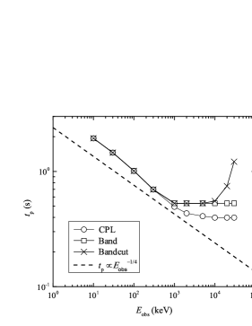
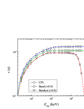
Figure 2: $t_{\rm p}-E_{\rm obs}$ (left panel) and $\tau-E_{\rm obs}$ (right panel) relations, where the situations with CPL, Band, and Bandcut radiation spectrum are shown with the symbols $\circ$, $\square$, and $\times$, respectively. In addition, the relation of $t_{\rm p}\propto\nu_{\rm obs}^{-0.25}$ is also plotted in the left panel (dashed line) for comparisons. The dashed lines in the right panel are well fitted by using Equation (16).

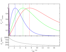
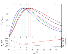
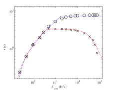
Figure 3: Left panel: the synthetic light curves (upper sub-figure) and the evolution of $E_{\rm ch}$ (lower sub-figure) for the case with CPL spectrum; Middle pane: the synthetic light curves (upper sub-figure) and the evolution of $E_{\rm p}$ ($E_{\rm c}$) (lower sub-figure) for the Bandcut case; Right panel: the $\tau-E_{\rm obs}$ relations with “$\circ$” for CPL case and “$\times$” for Bandcut case, respectively, and the red dashed lines are fitted by using Equation (16).

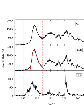
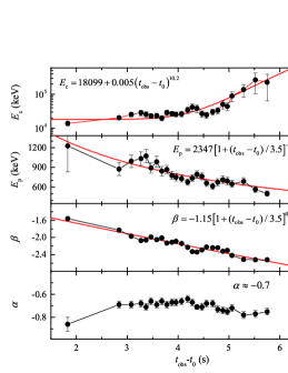
Figure 6: Left Panel: Light curve of GRB 160625B second sub-burst. Here, the two vertical dashed lines mark the time period for performing the cross-correlation function analysis, and the red curve in middle sub-figure is fitted by using Equation (13) and read as $I_{\rm p,f}=23804$ photons/s, $t_{0}=187.5$ s, $t_{\rm p,f}=189$ s, $\mathcal{R}=1.27$, and $\mathcal{D}=3.36$. Right Panel: The temporal evolution of $\alpha$, $\beta$, $E_{\rm p}$, and $E_{\rm c}$. The red solid lines in each sub-figure denote the fitting results with $t_{0}=185$ s.

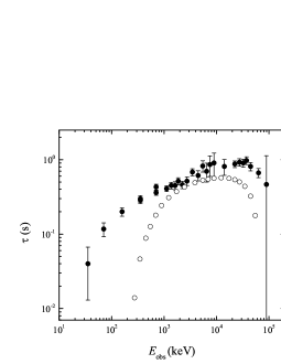
Figure 7: Right panel: $\tau-E_{\rm obs}$ relation for the first pulse in the GRB 160625B second sub-burst (black dots) and the numerical results of the spectral lag behavior in GRB 160625B by using the empirical model in Section 2.3 is denoted by the ‘$\circ$’ symbol.

Table 1: The time lags between the lowest energy band (10–25 keV) and any other high energy bands for the second sub-burst of GRB 160625B.

Energy	$\tau$	Energy	$\tau$
(keV)	(s)	(keV)	(s)
25–50	$0.04\pm 0.027$	5000–6000	$0.823\pm 0.141$
50–100	$0.117\pm 0.025$	6000–7000	$0.698\pm 0.199$
100–250	$0.2\pm 0.026$	7000–8000	$0.858\pm 0.262$
250–500	$0.298\pm 0.03$	8000–10000	$0.905\pm 0.32$
500–1000	$0.43\pm 0.038$	10000–20000	$0.81\pm 0.193$
1000–1250	$0.409\pm 0.036$	20000–25000	$0.873\pm 0.089$
1250–1500	$0.45\pm 0.045$	25000–30000	$0.923\pm 0.106$
1500–1750	$0.45\pm 0.055$	30000–35000	$0.904\pm 0.11$
1750–2000	$0.515\pm 0.056$	35000–40000	$0.976\pm 0.116$
2000–2500	$0.46\pm 0.052$	40000–50000	$0.811\pm 0.104$
2500–3000	$0.516\pm 0.067$	50000–80000	$0.666\pm 0.094$
3000–4000	$0.681\pm 0.073$	80000–100000	$0.465\pm 0.664$
4000–5000	$0.614\pm 0.097$

References

- Ackermann et al. (2011) Ackermann, M., Ajello, M., Asano, K., et al. 2011, ApJ, 729, 114
- Ackermann et al. (2013) Ackermann, M., Ajello, M., Asano, K., et al. 2013, ApJS, 209, 11
- Band et al. (1993) Band, D., Matteson, J., Ford, L., et al. 1993, ApJ, 413, 281
- Band (1997) Band, D. L. 1997, ApJ, 486, 928
- Baring & Harding (1997) Baring, M. G., & Harding, A. K. 1997, ApJ, 481, L85
- Bošnjak & Daigne (2014) Bošnjak, Ž., & Daigne, F. 2014, A&A, 568, A45
- Chang et al. (2008) Chang, P., Spitkovsky, A., & Arons, J. 2008, ApJ, 674, 378
- Chen et al. (2005) Chen, L., Lou, Y.-Q., Wu, M., et al. 2005, ApJ, 619, 983
- Cheng et al. (1995) Cheng, L. X., Ma, Y. Q., Cheng, K. S., Lu, T., & Zhou, Y. Y. 1995, A&A, 300, 746
- Daigne & Mochkovitch (2003) Daigne, F., & Mochkovitch, R. 2003, MNRAS, 342, 587
- Deng et al. (2016) Deng, W., Zhang, H., Zhang, B., et al. 2016, ApJ, 821, L12
- Fenimore et al. (1993) Fenimore, E. E., Epstein, R. I., & Ho, C. 1993, A&AS, 97, 59
- Fishman & Meegan (1995) Fishman, G. J., & Meegan, C. A. 1995, ARA&A, 33, 415
- Fraija (2015) Fraija, N. 2015, ApJ, 804, 105
- Fraija et al. (2016) Fraija, N., Lee, W. H., Veres, P., & Barniol Duran, R. 2016, ApJ, 831, 22
- Gao et al. (2012) Gao, H., Liang, N., & Zhu, Z.-H. 2012, International Journal of Modern Physics D, 21, 1250016-1-1250016-16
- Goodman (1986) Goodman, J. 1986, ApJ, 308, L47
- Gehrels et al. (2006) Gehrels, N., Norris, J. P., Barthelmy, S. D., et al. 2006, Nature, 444, 1044
- Ioka & Nakamura (2001) Ioka, K., & Nakamura, T. 2001, ApJ, 554, L163
- Keshet et al. (2009) Keshet, U., Katz, B., Spitkovsky, A., & Waxman, E. 2009, ApJ, 693, L127
- Kobayashi et al. (2007) Kobayashi, S., Zhang, B., Mészáros, P., & Burrows, D. 2007, ApJ, 655, 391
- Kocevski et al. (2003) Kocevski, D., Ryde, F., & Liang, E. 2003, ApJ, 596, 389
- Kouveliotou et al. (1993) Kouveliotou, C., Meegan, C. A., Fishman, G. J., et al. 1993, ApJ, 413, L101
- Krolik & Pier (1991) Krolik, J. H., & Pier, E. A. 1991, ApJ, 373, 277
- Lemoine et al. (2013) Lemoine, M., Li, Z., & Wang, X.-Y. 2013, MNRAS, 435, 3009
- Liang et al. (2006) Liang, E. W., Zhang, B., O’Brien, P. T., et al. 2006, ApJ, 646, 351
- Lin et al. (2018) Lin, D.-B., Lu, R.-J., Du, S.-S., et al. 2018, ApJ, submitted
- Lu et al. (2006) Lu, R.-J., Qin, Y.-P., Zhang, Z.-B., & Yi, T.-F. 2006, MNRAS, 367, 275
- Lu et al. (2018) Lu, R.-J., Liang, Y.-F., Lin, D.-B., et al. 2018, ApJ, 865, 153
- McBreen et al. (2008) McBreen, S., Foley, S., Watson, D., et al. 2008, ApJ, 677, L85
- Medvedev et al. (2005) Medvedev, M. V., Fiore, M., Fonseca, R. A., et al. 2005, ApJ, 618, L75
- Mészáros, & Rees (2000) Mészáros, P., & Rees, M. J. 2000, ApJ, 530, 292
- Norris et al. (1986) Norris, J. P., Share, G. H., Messina, D. C., et al. 1986, ApJ, 301, 213
- Norris et al. (2000) Norris, J. P., Marani, G. F., & Bonnell, J. T. 2000, ApJ, 534, 248
- Norris et al. (2001a) Norris, J. P., Scargle, J. D., & Bonnell, J. T. 2001, Gamma-ray Bursts in the Afterglow Era, 40
- Norris et al. (2001b) Norris, J. P., Scargle, J. D., & Bonnell, J. T. 2001, Gamma 2001: Gamma-Ray Astrophysics, 587, 176
- Norris (2004) Norris, J. P. 2004, Baltic Astronomy, 13, 221
- Norris et al. (2005) Norris, J. P., Bonnell, J. T., Kazanas, D., et al. 2005, ApJ, 627, 324
- Norris & Bonnell (2006) Norris, J. P., & Bonnell, J. T. 2006, ApJ, 643, 266
- Paczynski (1986) Paczynski, B. 1986, ApJ, 308, L43
- Pe’er (2015) Pe’er, A. 2015, Advances in Astronomy, 2015, 907321
- Peng et al. (2007) Peng, Z.-Y., Lu, R.-J., Qin, Y.-P., & Zhang, B.-B. 2007, Chinese J. Astron. Astrophys., 7, 428
- Peng et al. (2011) Peng, Z. Y., Yin, Y., Bi, X. W., Bao, Y. Y., & Ma, L. 2011, Astronomische Nachrichten, 332, 92
- Rees & Mészáros (1994) Rees, M. J., & Meszaros, P. 1994, ApJ, 430, L93
- Schaefer (2003) Schaefer, B. E. 2003, ApJ, 583, L67
- Schaefer (2007) Schaefer, B. E. 2007, ApJ, 660, 16
- Shao & Dai (2005) Shao, L., & Dai, Z. G. 2005, ApJ, 633, 1027
- Shao et al. (2017) Shao, L., Zhang, B.-B., Wang, F.-R., et al. 2017, ApJ, 844, 126
- Shen et al. (2005) Shen, R.-F., Song, L.-M., & Li, Z. 2005, MNRAS, 362, 59
- Shenoy et al. (2013) Shenoy, A., Sonbas, E., Dermer, C., et al. 2013, ApJ, 778, 3
- Silva et al. (2003) Silva, L. O., Fonseca, R. A., Tonge, J. W., et al. 2003, ApJ, 596, L121
- Tang et al. (2015) Tang, Q.-W., Peng, F.-K., Wang, X.-Y., & Tam, P.-H. T. 2015, ApJ, 806, 194
- Thompson (1994) Thompson, C. 1994, MNRAS, 270, 480
- Uhm & Zhang (2014) Uhm, Z. L., & Zhang, B. 2014, Nature Physics, 10, 351
- Uhm & Zhang (2015) Uhm, Z. L., & Zhang, B. 2015, ApJ, 808, 33
- Uhm & Zhang (2016a) Uhm, Z. L., & Zhang, B. 2016, ApJ, 824, L16
- Uhm & Zhang (2016b) Uhm, Z. L., & Zhang, B. 2016, ApJ, 825, 97
- Uhm et al. (2018) Uhm, Z. L., Zhang, B., & Racusin, J. 2018, arXiv:1801.09183
- Ukwatta et al. (2010) Ukwatta, T. N., Stamatikos, M., Dhuga, K. S., et al. 2010, ApJ, 711, 1073
- Ukwatta et al. (2012) Ukwatta, T. N., Dhuga, K. S., Stamatikos, M., et al. 2012, MNRAS, 419, 614
- Wei et al. (2017) Wei, J.-J., Zhang, B.-B., Shao, L., Wu, X.-F., & Mészáros, P. 2017, ApJ, 834, L13
- Woods & Loeb (1995) Woods, E., & Loeb, A. 1995, ApJ, 453, 583
- Xu et al. (2016) Xu, D., Malesani, D., Fynbo, J. P. U., et al. 2016, GRB Coordinates Network, Circular Service, No. 19600, #1 (2016), 19600, 1
- Yi et al. (2006) Yi, T., Liang, E., Qin, Y., & Lu, R. 2006, MNRAS, 367, 1751
- Zhang et al. (2009) Zhang, B., Zhang, B.-B., Virgili, F. J., et al. 2009, ApJ, 703, 1696
- Zhang & Yan (2011) Zhang, B., & Yan, H. 2011, ApJ, 726, 90
- Zhang et al. (2012) Zhang, B.-B., Burrows, D. N., Zhang, B., et al. 2012, ApJ, 748, 132
- Zhang et al. (2018) Zhang, B.-B., Zhang, B., Castro-Tirado, A. J., et al. 2018, Nature Astronomy, 2, 69
- Zhang et al. (2018) Zhang, B.-B., Zhang, B., Sun, H., et al. 2018, Nature Communications, 9, 447
- Zhao et al. (2014) Zhao, X., Li, Z., Liu, X., et al. 2014, ApJ, 780, 12