Circularly Symmetric Light Waves: An Overview

Abstract

Orbital Angular Momentum (OAM) waves were first recognized as those specific vortex solutions of the paraxial Helmholtz equation for which the orbital contribution to the total angular momentum of the beam yields an integer multiple of $\hbar$ along the propagation direction. However, this class of solutions can be generalized to include more sophisticated vector vortex waves with coupled polarization and spatial complexity, that are eigenfunctions of the third component of the angular momentum operator. In this work, a rigorous framework is proposed for the analysis of all the possible families of vortex solutions to the homogeneous Helmholtz equation. Both the scalar and vector cases are studied in depth, making use of an operator approach which emphasizes their intimate connection with the two-dimensional rotation group. Furthermore, a special focus is given to the characterization of the propagation properties of the most popular families of paraxial OAM beams.

1 Introduction

Electromagnetic waves carry energy and both linear and angular momenta. Whereas a contribution to the total angular momentum is realized by the spin of the photon, the fundamental physical quantity associated with polarization, an orbital angular momentum (OAM) component can also be present. Such contribution is often said to be “quasi-intrinsic” [1], since it is independent of the axis of calculation for any beam endowed with a helical wavefront apertured symmetrically about the beam axis [2]. The OAM content of helical beams in the paraxial regime was first discovered by Les Allen et al. in 1992 [3], although these waves have been known for much longer in terms of optical vortices and are now often referred to as vortex waves. OAM beams are characterized by an azimuthal phase dependence of the form $\exp\left(im\varphi\right)$, where the integer $m$ represents the topological charge of the vortex (or, more simply, the number of intertwined helices the wavefront is made of) and is related to the OAM carried by the beam along the propagation axis. For $m\neq 0$, due to the presence of the on-axis phase singularity, scalar OAM waves present a doughnut-shaped intensity profile with a central null.

It would seem natural to think that, being the OAM a global property of the beam in contrast to the spin angular momentum (SAM), the orbital and spin contributions to the total angular momentum of an electromagnetic wave are two distinct quantities. However, it has been argued that, in view of the absence of any rest frame for the photon, a gauge-invariant decomposition of the total electromagnetic angular momentum in orbital and spin parts is unfeasible (see for example [4, 5]) or achievable at most within the paraxial limit [6], the polarization and spatial degrees of freedom being in general coupled. Despite these arguments, Steven J. van Enk and Gerald Nienhuis have claimed that it is indeed possible to extract gauge-independent expressions for the spin and orbital parts of the angular momentum, but neither of these contributions alone represents a true angular momentum, since the transversality of the radiation fields affects the commutation relations for the associated quantum operators [7]. Such interpretation proves to be the currently accepted one [8].

The first experimental proof of an angular momentum transfer between light and matter dates back to 1936, when Richard A. Beth verified the interaction between a circularly polarized beam and a quarter-wave plate [9]: owing to the photon spin, the torque exerted by the polarized radiation on the plate put it into rotation. Since then, a great number of similar experiments have been performed, also involving the use of OAM beams. The angular momentum of light can be transferred to suitable trapped material particles causing them to rotate [10, 11], with relevant applications in both micromanipulation and the design and operation of micromachines [12, 13, 14, 15]. Vortex waves are also used as a tool for advanced cell manipulation [16] and to transport aqueous droplets in solution [17]. Moreover, direct transfer of OAM from light to atoms in ultracold gas clouds has been reported [18, 19, 20].

The interest in OAM waves extends far beyond the light-matter angular momentum exchange and several attractive applications can be found in optics, quantum physics and astronomy. For instance, light vortices are employed to probe different physical and biological properties of matter in optical imaging [21, 22, 23], but also for encoding quantum information via the corresponding photon states in high-dimensional Hilbert spaces [24, 25, 26, 27, 28]. OAM beams are involved in second harmonic generation processes [29, 30, 31] as well as in many other nonlinear optics phenomena [32, 33, 34, 35], being intended in terms of vortex solitons [36, 37, 38]. Further possibilities lie in the use of vortex waves to enhance the resolution in quantum imaging [39] and for overcoming the Rayleigh limit of the telescopes [40], whereas several other interesting studies are reported by the astrophysical community [41, 42, 43, 44, 45]. Many of the so far described applications together with other examples and a more complete list of references can be found in [46, 47, 48, 49, 50, 51].

Currently, a large part of the research on OAM beams is also devoted to the field of telecommunications. From a strictly mathematical point of view, vortex waves represent classes of solutions to the Helmholtz equation; since each class comprises a set of orthogonal solutions, in 2004 Graham Gibson et al. proposed the idea of using such waves to convey independent information channels on a single frequency in free-space optical communication links [52]. The authors also suggested how the intrinsic sensitivity of the OAM orthogonality to angular restrictions and lateral offsets [53] could prevent eavesdropping.

In these last few years, a strong interest in the possibility to increase the communication efficiency by vortex waves is growing [54, 55, 56, 57, 58, 59, 60] and has also been extended to the radio frequency domain [61, 62, 63, 64, 65]. In this scenario, however, the degree of innovation of OAM multiplexing with respect to other existing techniques like those based on antenna diversity and, more generally, on the use of orthogonal wavefields has been questioned [66, 67, 68, 69, 70, 71, 72].

Motivated by the astonishing amount of OAM-related publications, a theoretical study is proposed in this paper on the mathematical features of free-space vortex waves. While presenting new results and general insights that can be of interest to the optics community, a large part of the literature on this fascinating topic is carefully reviewed. In Section 2, a detailed overview on the scalar OAM waves is outlined, starting from some basic results of group theory. In Section 3, the fundamental solutions of the paraxial Helmholtz equation are derived step by step through an ansatz approach and their propagation properties are systematically analyzed. In Section 4, the vector case is studied in depth from a new perspective and some well-known examples are revisited accordingly. The last section is devoted to the conclusions. Further calculations are reported in appendix as a support to the main text.

2 Vortex solutions of the scalar wave equation

As it is known in group theory, separable coordinate systems for second-order linear partial differential equations can be characterized in terms of sets of operators in the algebra relative to the underlying continuous symmetry group [73]. In this framework, the separated solutions of the considered equations are common eigenfunctions of the symmetry operators and the expansion of one set of separable solutions in terms of another leads back to a problem in the representation theory of the Lie algebra. The Helmholtz wave equation, one of the most studied examples, is proven to be separable in eleven three-dimensional coordinate systems [74]: Cartesian, circular cylindrical, elliptic cylindrical, parabolic cylindrical, spherical, prolate spheroidal, oblate spheroidal, parabolic, ellipsoidal, paraboloidal and conical. In optics, solutions of the Helmholtz equation which are eigenfunctions of the Lie algebra generator of the translations along the $z$-coordinate are usually considered, since only for them the equation can be separated into transverse and longitudinal parts; actually, this condition is satisfied in the first four orthogonal coordinate systems.

A useful approach for building a formal description of OAM waves is to analyze their definition from a very general point of view, proceeding along the lines of the methods and techniques developed in group theory. The fundamental feature which has been referred to in defining vortex waves from the very beginning is indeed represented by the aforementioned screw phase dislocation $\exp\left(im\varphi\right)$, whose presence is soon recognized as the footprint of the underlying circular symmetry. In particular, given a fixed axis along the unit vector $\mathbf{u}_{z}$, rotations about this axis form a one-parameter subgroup of SO(3) which is isomorphic to the group of rotations in the plane perpendicular to $\mathbf{u}_{z}$, that is SO(2) [75]. Through the azimuthal integer index $m$, the function $\varPhi_{m}\left(\varphi\right)=\exp\left(im\varphi\right)$ is known to span the set of single-valued irreducible representations of SO(2), for which the following orthogonality and completeness relations hold:

$$\frac{1}{2\pi}\int_{0}^{2\pi}\varPhi_{j}^{*}\left(\varphi\right)\varPhi_{m}\left(\varphi\right)\,d\varphi=\delta_{jm};\quad\sum_{m}\varPhi_{m}\left(\varphi\right)\varPhi_{m}^{*}\left(\varphi^{\prime}\right)=\delta\left(\varphi-\varphi^{\prime}\right).$$ (1)

Associated with the subgroup algebra there is a generator, $\hat{J}_{z}$, and all elements of the given subgroup can be written symbolically as $\exp\left(\varphi\hat{J}_{z}\right)$, where $\varphi$ parameterizes the rotation.

A basis for the Lie algebra of SO(3) in standard matrix representation is provided by the three operators:

$$J_{1}=\left[\begin{array}[]{ccc}0&0&0\\ 0&0&-1\\ 0&1&0\end{array}\right];\quad J_{2}=\left[\begin{array}[]{ccc}0&0&1\\ 0&0&0\\ -1&0&0\end{array}\right];\quad J_{3}=\left[\begin{array}[]{ccc}0&-1&0\\ 1&0&0\\ 0&0&0\end{array}\right],$$ (2)

which obey the commutation relations $\left[J_{s},\,J_{v}\right]={\varepsilon_{sv}}^{k}J_{k}$, where $\varepsilon_{svk}$ is the Levi-Civita pseudo-tensor and the Einstein summation convention has been considered; in (2), the subscripts $1$, $2$ and $3$ denote Cartesian components $x$, $y$ and $z$, respectively. Although the origin of these commutation relations is really geometric in nature, the generators acquire even more significance in quantum physics, where they correspond to measurable quantities [76]. In this respect, $\mathbf{J}=\left(J_{1},J_{2},J_{3}\right)$ can be seen as the vector angular momentum operator in units of $\hbar$.

Whereas the matrix representation is widely used to express the SAM operator, a differential representation is often preferable to (2) for describing the OAM operator. As suggested in [77], analogies between quantum mechanics and scalar paraxial optics can be built in order to demonstrate heuristically that some cylindrical laser modes with a $\varPhi_{m}\left(\varphi\right)$ azimuthal phase dependence carry an OAM of $m\hbar$ per photon along the propagation axis.

Let us consider an arbitrary coordinate system $\left\{x_{1},x_{2},x_{3}\right\}$ and a free-space monochromatic scalar wave of the form $\Psi\left(x_{1},x_{2},x_{3},t\right)=\psi\left(x_{1},x_{2},x_{3}\right)\mathrm{e}^{i\omega t}$, where $\omega=kc$ represents the angular frequency, $k=2\pi/\lambda$ the wavenumber, $\lambda$ the wavelength and $c$ the speed of light. Even if the full vector nature of the electromagnetic radiation is being neglected at present, $\Psi\left(x_{1},x_{2},x_{3},t\right)$ can be understood as the amplitude of a linearly polarized electric field or vector potential, which satisfies the wave equation:

$$\nabla^{2}\Psi\left(x_{1},x_{2},x_{3},t\right)-\frac{1}{c^{2}}\frac{\partial^{2}}{\partial t^{2}}\Psi\left(x_{1},x_{2},x_{3},t\right)=0,$$ (3)

as follows from Maxwell theory. From (3), the scalar Helmholtz equation for the spatial coordinates dependent amplitude $\psi\left(x_{1},x_{2},x_{3}\right)$ is soon derived:

$$\nabla^{2}\psi\left(x_{1},x_{2},x_{3}\right)+k^{2}\psi\left(x_{1},x_{2},x_{3}\right)=0.$$ (4)

We are now interested in solutions $\psi$ to (4) that are eigenfunctions of the $\hat{J}_{z}$ operator, namely:

$$i\hat{J}_{z}\psi=-i\frac{\partial}{\partial\varphi}\psi=m\psi\quad\Rightarrow\quad\psi\left(x_{1},\varphi,x_{3}\right)=\varPhi_{m}\left(\varphi\right)u\left(x_{1},x_{3}\right),$$ (5)

where $\left\{x_{1},\varphi,x_{3}\right\}$ is a suitable coordinate system and the differential expression of the $\hat{J}_{z}$ operator has been introduced. It is important to note that the condition of periodicity of the wavefunction in the azimuthal coordinate imposes integer values for the $m$ index. In (5), $\varPhi_{m}\left(\varphi\right)$ corresponds to the sought vortex term and $u\left(x_{1},x_{3}\right)$ is a function obeying the reduced equation in the remaining two variables:

$$\frac{1}{h_{1}h_{\varphi}h_{3}}\left[\frac{\partial}{\partial x_{1}}\left(\frac{h_{\varphi}h_{3}}{h_{1}}\frac{\partial u}{\partial x_{1}}\right)+\frac{\partial}{\partial x_{3}}\left(\frac{h_{1}h_{\varphi}}{h_{3}}\frac{\partial u}{\partial x_{3}}\right)\right]+\left(k^{2}-\frac{m^{2}}{h_{\varphi}^{2}}\right)u=0,$$ (6)

being $h_{1}$, $h_{\varphi}$ and $h_{3}$ three $\varphi$-independent metric scale factors for the given coordinates [74].

It can be shown that (6) separates in five coordinate systems: circular cylindrical, spherical, prolate spheroidal, oblate spheroidal and parabolic [73]. While leaving to the appendix a formal proof of the equation separation in the latter four systems, let us focus in detail on the circular cylindrical case $\left\{\rho,\varphi,z\right\}$, for which equation (6) reads:

$$\left[\frac{\partial^{2}}{\partial\rho^{2}}+\frac{1}{\rho}\frac{\partial}{\partial\rho}-\frac{m^{2}}{\rho^{2}}+\frac{\partial^{2}}{\partial z^{2}}+k^{2}\right]u\left(\rho,z\right)=0.$$ (7)

As pointed out above, it is common to look for solutions of the Helmholtz equation that are eigenfunctions of the $\hat{P}_{z}$ operator, i.e. the generator of the translations along the $z$-axis:

$$\hat{P}_{z}u=\frac{\partial}{\partial z}u=-ik_{z}u\quad\Rightarrow\quad u\left(\rho,z\right)=B\left(\rho\right)e^{-ik_{z}z},$$ (8)

where $B\left(\rho\right)$ represents a function to be determined. The imposed condition implies a further reduction of equation (7):

$$\left[\frac{\partial^{2}}{\partial\rho^{2}}+\frac{1}{\rho}\frac{\partial}{\partial\rho}-\frac{m^{2}}{\rho^{2}}+\left(k^{2}-k_{z}^{2}\right)\right]B\left(\rho\right)=0.$$ (9)

After some straightforward manipulations, (9) is easily recognized as the Bessel equation (see, for instance, [78]) and thus $B\left(\rho\right)=J_{\left|m\right|}\left(k_{\rho}\rho\right)$, where $k^{2}=k_{\rho}^{2}+k_{z}^{2}$.

Scalar modes of the form:

$$\varPsi_{m}^{B}\left(\rho,\varphi,z,t;k_{\rho}\right)=C_{m}^{B}J_{\left|m\right|}\left(k_{\rho}\rho\right)\varPhi_{m}\left(\varphi\right)\exp\left(-ik_{z}z+i\omega t\right),$$ (10)

where $C_{m}^{B}$ is a suitable dimensional constant, are known as Bessel beams (BBs) and represent a complete set of orthogonal solutions to (3). The transverse intensity and phase profiles of a representative BB are displayed in Figure 1 for different values of the topological charge $m$.

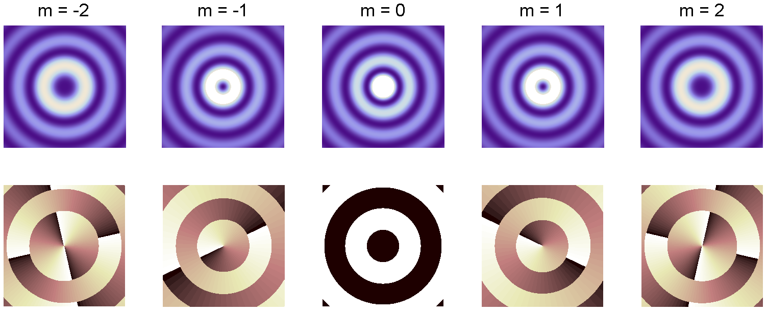
Figure 1: BB intensity (upper row) and phase (lower row) transverse profiles ($y$-coordinate versus $x$-coordinate) for $k_{\rho}=k/\sqrt{2}$.

As will be shown further on, BBs also satisfy the paraxial wave equation. Due to their divergence-free profile, the Bessel modes belong to the family of “non-diffracting” beams [79], which are not square-integrable and thus carry infinite energy; for this reason, only truncated forms of such waves can be realized experimentally. Physical OAM waves that approximate the intensity distribution of these ideal beams are usually produced via computer generated holograms [80] or axicons [81].

It is important to emphasize that, despite the leading role played by the circular cylindrical coordinate system in optics, BBs are not the only possible scalar OAM solutions and waves with a vortex term $\varPhi_{m}\left(\varphi\right)$ are also found by separating the Helmholtz equation in spherical, prolate spheroidal, oblate spheroidal and parabolic coordinates (see A for further details). In [82], an estimation of the electromagnetic OAM has also been performed for Mathieu beams, which can be intended as a generalization of BBs to elliptic cylindrical coordinates; in this case, however, the $\varPhi_{m}\left(\varphi\right)$ term cannot be present due to symmetry considerations and this results in the appearance of a more complicated vortex structure with fractional OAM mean content.

The presence of a non-integer OAM per photon in connection with some sort of symmetry breaking is a fact, by the way, not new, that leads to possible extensions of the simple original definition of OAM waves in several interesting scenarios [83, 84, 85, 86, 87, 88, 89, 90]. As a related topic, it should be noted that the very concept of wave vorticity is not limited to the isotropic case, which has been taken as a working hypothesis in defining OAM beams as vortex solutions. In particular, a vortex is said to be isotropic when the phase increases linearly from $0$ to $2\pi m$ around a circle enclosing the singularity [91, 92]; in this case, the iso-intensity contour lines are exact circles and the usual $\varPhi_{m}\left(\varphi\right)$ term is found. However, vortices are in general anisotropic, meaning that the intensity contours close to the singularities are elliptical [93, 94, 95, 96, 97, 98]. The anisotropic vortex can be understood as a geometrical deformation of the isotropic one, with an angular dependence of the form:

$$\widetilde{\varPhi}_{m}\left(\varphi\right)=\sqrt{2}\left\{\cos\epsilon\cos\left[m\left(\varphi-\varphi_{0}\right)\right]+i\sin\epsilon\sin\left[m\left(\varphi-\varphi_{0}-\sigma\right)\right]\right\},$$ (11)

where $\epsilon$ represents the vortex anisotropy, $\sigma$ is the vortex skewness and $\varphi_{0}$ the vortex rotation angle. The possibility of representing anisotropic dislocations through a superposition of isotropic ones, as reported in [98], provides an easy derivation of the expectation value and the uncertainty of the OAM.

A further aspect to be mentioned lies in the non-existence of propagating solutions characterized by a term $\varPhi_{\mu}\left(\varphi\right)$ with non-integer $\mu$ index: when programmed to have a non-integer phase dislocation of this form as a starting condition, electromagnetic beams evolve with the creation of a group of standard vortices which break the circular symmetry of the intensity profile. Such mechanism and all the related topics have been deeply explored and characterized [83, 84, 86, 87, 92].

The study of the electromagnetic vortices and their dynamics and interactions belong to the rich field of the singular optics, to which reference should be made. In spite of all the possible generalizations that can be introduced in the definition of OAM waves as vortex solutions, only the original requirement, i.e. the presence of an on-axis isotropic vortex, will be taken into account, since a complete classification would fall beyond the scope of the paper.

3 Paraxial OAM waves

In the event that the angle between the wavevector $\mathbf{k}$ and the propagation direction ($z$-axis) is small and assuming a beam amplitude of the form $\psi\left(\rho,\varphi,z\right)=f\left(\rho,\varphi,z\right)\exp\left(-ikz\right)$, where $f\left(\rho,\varphi,z\right)$ represents a slowly varying function of the $z$-coordinate, such that:

$$\left|\frac{\partial^{2}f\left(\rho,\varphi,z\right)}{\partial z^{2}}\right|\ll k\left|\frac{\partial f\left(\rho,\varphi,z\right)}{\partial z}\right|;\quad\left|\frac{\partial^{2}f\left(\rho,\varphi,z\right)}{\partial z^{2}}\right|\ll\left|\nabla_{T}^{2}\>f\left(\rho,\varphi,z\right)\right|,$$ (12)

being $\nabla_{T}^{2}$ the transverse Laplacian, equation (4) reduces to its paraxial version [99]:

$$\left[\frac{\partial^{2}}{\partial\rho^{2}}+\frac{1}{\rho}\frac{\partial}{\partial\rho}+\frac{1}{\rho^{2}}\frac{\partial^{2}}{\partial\varphi^{2}}-2ik\frac{\partial}{\partial z}\right]f\left(\rho,\varphi,z\right)=0.$$ (13)

The paraxial Helmholtz equation (13) is widely used in optics, where the above described requirements are usually met and it represents a complete enough approximation to handle transverse variations and diffraction effects of the optical beam profile [100]. The reported equation is of the Schrödinger type and proves to admit solutions with separable variables in seventeen coordinate systems [73].

A huge amount of publications regarding the analytical derivation of families of paraxial beams can be found in the literature [101, 102, 103, 104, 105, 106, 107, 108, 109, 110, 111, 112, 113, 114, 115, 116, 117, 118, 119, 120, 121, 122, 123, 124, 125, 126, 127, 128, 129]. The most general set of solutions of (13) in circular cylindrical coordinates has been obtained and characterized recently [105, 107]; closed form expressions are provided in terms of the confluent hypergeometric functions [78]. Among all special cases of the paraxial vortex waves, some cylindrical families are of particular relevance and will be analyzed by means of an intuitive ansatz approach [130].

First, in order to simplify the notation, it is useful to introduce a set of dimensionless circular cylindrical coordinates $\left\{\varrho,\varphi,\zeta\right\}=\left\{\rho/w_{0},\varphi,z/z_{R}\right\}$, where $z_{R}=\pi w_{0}^{2}/\lambda$ and $w_{0}$ corresponds to a characteristic length parameter for the beam. Equation (13) then becomes:

$$\left[\frac{\partial^{2}}{\partial\varrho^{2}}+\frac{1}{\varrho}\frac{\partial}{\partial\varrho}+\frac{1}{\varrho^{2}}\frac{\partial^{2}}{\partial\varphi^{2}}-4i\frac{\partial}{\partial\zeta}\right]f\left(\varrho,\varphi,\zeta\right)=0.$$ (14)

For cylindrical beams satisfying the requirements of the paraxial approximation it is useful to appeal to the following ansatz, which is eigenfunction of the $\hat{J}_{z}$ operator by definition:

$$f\left(\varrho,\varphi,\zeta\right)=\frac{C}{\mu\left(\zeta\right)}u\left[\frac{\varrho}{\mu\left(\zeta\right)},\zeta\right]\exp\left[i\phi\left(\zeta\right)\frac{\varrho^{2}}{\mu^{2}\left(\zeta\right)}+im\varphi\right],$$ (15)

where $\mu\left(\zeta\right)$ and $\phi\left(\zeta\right)$ are two dimensionless functions which account for the diffraction effects, $m\in\mathbb{Z}$ represents the topological charge of the on-axis vortex and $C$ is a constant. By inserting expression (15) into (14), a partial differential equation for the function $u\left(r,\zeta\right)$ is found which can be put in the form of a $\zeta$-dependent Schrödinger equation:

$$i\frac{\partial u\left(r,\zeta\right)}{\partial\zeta}=\hat{H}\left(\zeta\right)u\left(r,\zeta\right)$$ (16)

with Hamiltonian given by:

$$\hat{H}\left(\zeta\right) = \frac{1}{4\mu^{2}\left(\zeta\right)}\left\{\hat{P}+4\left[\mu\left(\zeta\right)\frac{d\mu\left(\zeta\right)}{d\zeta}+\phi\left(\zeta\right)\right]\hat{Q}-\frac{m^{2}}{r^{2}}\right\}$$ (17)

$$+ r^{2}\left[\frac{d\phi\left(\zeta\right)}{d\zeta}-\frac{\phi^{2}\left(\zeta\right)}{\mu^{2}\left(\zeta\right)}-\frac{2\phi\left(\zeta\right)}{\mu\left(\zeta\right)}\frac{d\mu\left(\zeta\right)}{d\zeta}\right],$$

where the following two operators have been introduced:

$$\hat{P}=\frac{\partial^{2}}{\partial r^{2}}+\frac{1}{r}\frac{\partial}{\partial r};\quad\hat{Q}=i\left(r\frac{\partial}{\partial r}+1\right).$$ (18)

As will be shown further on, a simple characterization of the cylindrical paraxial OAM beams can be derived from the definitions:

$$a=\mu\frac{d\mu}{d\zeta}+\phi;\quad b=\mu^{2}\left[\frac{d\phi}{d\zeta}-\frac{\phi^{2}}{\mu^{2}}-\frac{2\phi}{\mu}\frac{d\mu}{d\zeta}\right],$$ (19)

which allow to rewrite equation (16) as:

$$i\frac{\partial u\left(r,\zeta\right)}{\partial\zeta}=\left\{\frac{1}{4\mu^{2}\left(\zeta\right)}\left[\hat{P}+4a\hat{Q}-\frac{m^{2}}{r^{2}}\right]+\frac{br^{2}}{\mu^{2}\left(\zeta\right)}\right\}u\left(r,\zeta\right).$$ (20)

It is interesting to note that both $\hat{P}$ and $\hat{Q}$ are Hermitian operators with respect to the integration measure $rdr$, therefore the Hamiltonian $\hat{H}\left(\zeta\right)$ (term in braces in the above expression) is Hermitian if $a,\>b\in\mathbb{R}$ and $\mu^{2}\left(\zeta\right)$ corresponds to a real valued function of the $\zeta$-coordinate: in this particular case, complete sets of orthogonal solutions are obtained for the stationary Schrödinger equation. These and other classes of solutions are derived from the choice of the parameters $a$, $b$ and by establishing suitable functions $\mu\left(\zeta\right)$, $\phi\left(\zeta\right)$ which satisfy (19).

3.1 Bessel beams

With the choice $a=b=0$, $\mu\left(\zeta\right)=1$ and $\phi\left(\zeta\right)=0$, equation (20) reads:

$$i\frac{\partial u_{B}\left(r,\zeta\right)}{\partial\zeta}=\frac{1}{4}\left[\frac{\partial^{2}}{\partial r^{2}}+\frac{1}{r}\frac{\partial}{\partial r}-\frac{m^{2}}{r^{2}}\right]u_{B}\left(r,\zeta\right),$$ (21)

where the subscript $B$ has been introduced; alternatively, going back to the original coordinate system:

$$ik\frac{\partial u_{B}\left(\rho,z\right)}{\partial z}=\frac{1}{2}\left[\frac{\partial^{2}}{\partial\rho^{2}}+\frac{1}{\rho}\frac{\partial}{\partial\rho}-\frac{m^{2}}{\rho^{2}}\right]u_{B}\left(\rho,z\right).$$ (22)

For a paraxial beam of the form $\psi_{B}\left(\rho,\varphi,z\right)=g_{B}\left(\rho,\varphi,z\right)\exp\left(-ik_{z}z\right)$, the following relation holds:

$$k_{z}=\sqrt{k^{2}-k_{x}^{2}-k_{y}^{2}}\approx k-\frac{k_{\rho}^{2}}{2k},$$ (23)

where $k_{\rho}^{2}=k_{x}^{2}+k_{y}^{2}$. Then we can write $\psi_{B}\left(\rho,\varphi,z\right)=f_{B}\left(\rho,\varphi,z\right)\exp\left(-ikz\right)$ with $f_{B}\left(\rho,\varphi,z\right)=g_{B}\left(\rho,\varphi,z\right)\exp\left(ik_{\rho}^{2}z/2k\right)$. Taking into account expression (15), we infer:

$$u_{B}\left(\rho,z\right)\propto B\left(\rho\right)\exp\left(i\frac{k_{\rho}^{2}z}{2k}\right),$$ (24)

which, substituted in equation (22), gives:

$$\rho^{2}\frac{d^{2}B\left(\rho\right)}{d\rho^{2}}+\rho\frac{dB\left(\rho\right)}{d\rho}+\left(\rho^{2}k_{\rho}^{2}-m^{2}\right)B\left(\rho\right)=0.$$ (25)

Equation (25) corresponds exactly to (9) and, as mentioned above, its regular solution $B\left(\rho\right)$ is provided by the Bessel function of the first kind $J_{\left|m\right|}\left(k_{\rho}\rho\right)$, therefore leading to:

$$f_{m}^{B}\left(\rho,\varphi,z;k_{\rho}\right)=C_{m}^{B}J_{\left|m\right|}\left(k_{\rho}\rho\right)\exp\left(i\frac{k_{\rho}^{2}z}{2k}+im\varphi\right).$$ (26)

The paraxial modes $\Psi_{m}^{B}\left(\rho,\varphi,z,t;k_{\rho}\right)=f_{m}^{B}\left(\rho,\varphi,z;k_{\rho}\right)\mathrm{e}^{-ikz+i\omega t}$ are nothing but the above discussed BBs (10). By virtue of their completeness and of the fact that they satisfy both the exact and the paraxial wave equations, BBs are well suited for implementing non-paraxial extensions of known beams families which belong originally to the set of paraxial solutions [48].

3.2 Laguerre-Gaussian beams

Let now $a=0$, $b=-1$, $\mu\left(\zeta\right)=\sqrt{1+\zeta^{2}}$ and $\phi\left(\zeta\right)=-\zeta$:

$$i\frac{\partial u_{LG}\left(r,\zeta\right)}{\partial\zeta}=\frac{1}{4\mu^{2}\left(\zeta\right)}\left[\frac{\partial^{2}}{\partial r^{2}}+\frac{1}{r}\frac{\partial}{\partial r}-\frac{m^{2}}{r^{2}}-4r^{2}\right]u_{LG}\left(r,\zeta\right).$$ (27)

In order to solve equation (27), it is convenient to start from the following assumption:

$$u_{LG}\left(r,\zeta\right)\propto r^{\left|m\right|}LG\left(2r^{2}\right)\exp\left[-r^{2}-i\Theta\left(\zeta\right)\right],$$ (28)

where $LG\left(2r^{2}\right)$ and $\Theta\left(\zeta\right)$ are functions to be determined. After some straightforward algebraic steps, equation (27) reduces to:

$$4r^{\left|m\right|+2}\left(LG^{{}^{\prime\prime}}-LG^{{}^{\prime}}\right)+r^{\left|m\right|}\left\{2\left(\left|m\right|+1\right)LG^{{}^{\prime}}-\left[\left|m\right|+1+\mu^{2}\frac{d\Theta}{d\zeta}\right]LG\right\}=0,$$ (29)

with the definitions $LG^{{}^{\prime}}=dLG\left(x\right)/dx$ and $LG^{{}^{\prime\prime}}=d^{2}LG\left(x\right)/dx^{2}$. Since an equation which holds for every $\zeta$ is needed, the coefficient with $\zeta$-dependence must be set equal to a constant, a conventional choice being $-\left(2p+\left|m\right|+1\right)$, with $p\in\mathbb{N}$:

$$\left|m\right|+1+\mu^{2}\left(\zeta\right)\frac{d\Theta\left(\zeta\right)}{d\zeta}=-2p.$$ (30)

The equation is easily solved and gives:

$$\Theta\left(\zeta\right)=-\left(2p+\left|m\right|+1\right)\arctan\left(\zeta\right).$$ (31)

Hence, expression (29) becomes:

$$2r^{2}LG^{{}^{\prime\prime}}\left(2r^{2}\right)+\left(\left|m\right|+1-2r^{2}\right)LG^{{}^{\prime}}\left(2r^{2}\right)+pLG\left(2r^{2}\right),$$ (32)

whose regular solution is the generalized Laguerre polynomial $L_{p}^{\left|m\right|}\left(2r^{2}\right)$ [78] and leads to:

$$f_{pm}^{LG}\left(\rho,\varphi,z\right) = \frac{C_{pm}^{LG}}{w\left(z\right)}\left[\frac{\rho}{w\left(z\right)}\right]^{\left|m\right|}L_{p}^{\left|m\right|}\left[\frac{2\rho^{2}}{w^{2}\left(z\right)}\right]\exp\left(im\varphi\right)$$ (33)

$$\times \exp\left[-\frac{\rho^{2}}{w_{0}^{2}\left(1-i\frac{z}{z_{R}}\right)}-i\Theta\left(\frac{z}{z_{R}}\right)\right].$$

In expression (33), the definition $w\left(z\right)=w_{0}\,\mu\left(z/z_{R}\right)$ has been introduced, $w_{0}$ corresponds to the waist of the Gaussian beam, $z_{R}$ is the Rayleigh distance (see Figure 2) and $\Theta\left(\zeta\right)$ the Gouy phase [100].

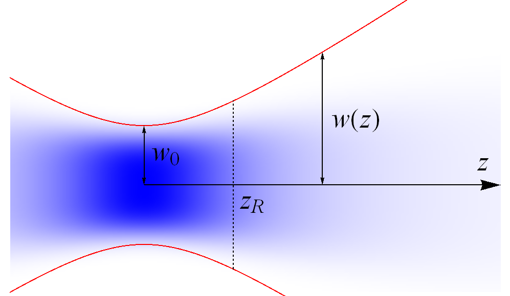
Figure 2: Propagation of the fundamental Gaussian wave $\psi_{00}^{LG}$: longitudinal intensity profile with some beam parameters.

The constant term $C_{pm}^{LG}$ ensures correct dimension and normalization of the beam profile.

The cylindrical modes $\Psi_{pm}^{LG}\left(\rho,\varphi,z,t\right)=f_{pm}^{LG}\left(\rho,\varphi,z\right)\mathrm{e}^{-ikz+i\omega t}$ are named Laguerre-Gaussian (LG) beams and represent another complete set of orthogonal paraxial OAM solutions of the scalar wave equation. The transverse intensity and phase profiles of a representative LG beam are displayed in Figure 3 for different values of the topological charge $m$. Unlike BBs, the LG modes diverge during propagation (in this regard, $z_{R}$ can be seen as the diffraction scale), they are spatially confined and carry a finite amount of energy, therefore can be physically realized, at least up to some degree of accuracy.

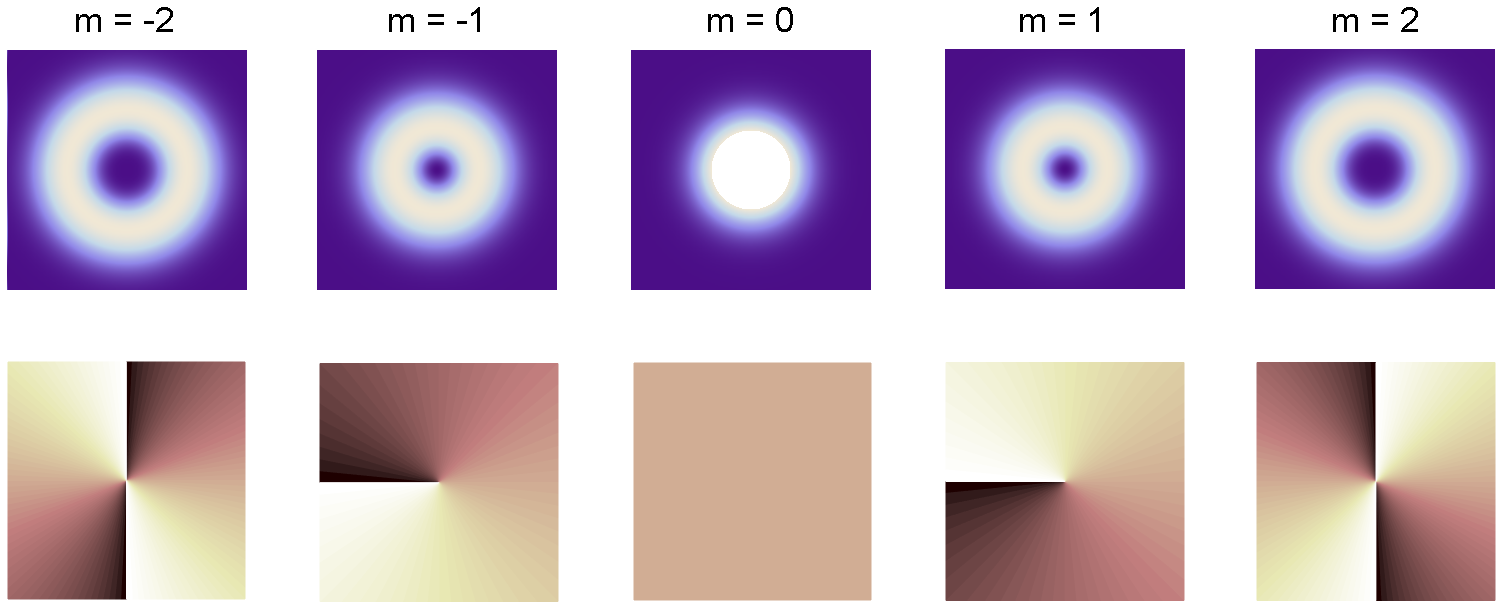
Figure 3: LG beam intensity (upper row) and phase (lower row) transverse profiles ($y$-coordinate versus $x$-coordinate) for $p=0$.

LG beams are shape-invariant modes: during free propagation, their intensity profile maintains the same shape and it is just scaled owing to diffraction and energy conservation. The radius of the primary intensity maximum evolves with $z$ according to the law:

$$\rho_{max}^{LG}\left(z\right)=\rho_{max,0}^{LG}\,\sqrt{1+\left(\frac{z}{z_{R}}\right)^{2}},$$ (34)

where $\rho_{max,0}^{LG}=\rho_{max}^{LG}\left(0\right)$ vanishes for $m=0$. At large distances, for $m\neq 0$, we infer $\rho_{max}^{LG}\left(z\right)\propto z$. By replacing $\rho$ with expression (34) in the square modulus of (33), we easily get:

$$I_{max}^{LG}\left(z\right)=\left|f_{pm}^{LG}\left[\rho_{max}^{LG}\left(z\right),\varphi,z\right]\right|^{2}=I_{max,0}^{LG}\left[1+\left(\frac{z}{z_{R}}\right)^{2}\right]^{-1},$$ (35)

being $I_{max,0}^{LG}=I_{max}^{LG}\left(0\right)$ the maximum intensity of the original profile. Therefore, for $z\gg z_{R}$, the asymptotic behavior $I_{max}^{LG}\left(z\right)\propto z^{-2}$ is obtained, as shown in Figure 4.

Let us now consider the decay of the intensity of a LG beam at a fixed radial coordinate $\bar{\rho}$ (for $m=0$, this also includes the case of the primary maximum at $\bar{\rho}=0$); the square modulus of (33) is given by:

$$I_{LG}\left(z\right)=\left|f_{pm}^{LG}\left[\bar{\rho},\varphi,z\right]\right|^{2}\propto\left[w^{2}\left(z\right)\right]^{-\left|m\right|-1}\left|L_{p}^{\left|m\right|}\left[\frac{2\bar{\rho}^{2}}{w^{2}\left(z\right)}\right]\right|^{2}\mathrm{e}^{-\frac{2\bar{\rho}^{2}}{w^{2}\left(z\right)}}.$$ (36)

For large enough distances, the term which contains the Laguerre polynomial tends to a constant and so does the exponential one, thus implying an asymptotic behavior of the form $I_{LG}\left(z\right)\propto z^{-2\left|m\right|-2}.$ The same law also describes the far-field evolution of the LG beam power collected on a central surface of limited size placed at distance $z$, reported in Figure 5.

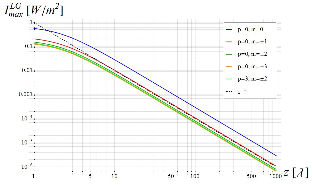
Figure 4: Evolution of the principal intensity maximum of some LG beams as a function of the propagation distance for $w_{0}=\lambda$.

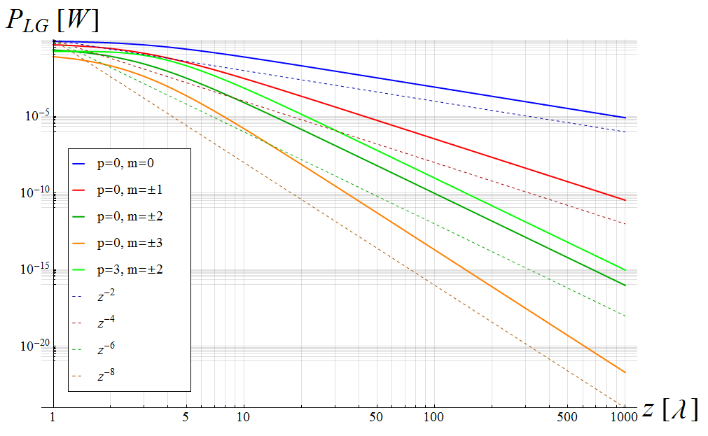
Figure 5: Evolution of the integral of the intensity of some LG beams over a centered circular region with radius $w_{0}$ as a function of $z$, for $w_{0}=\lambda$.

3.3 Hypergeometric beams

By choosing $a=-1/2$, $b=0$, $\mu\left(\zeta\right)=\sqrt{-\zeta}$ and $\phi\left(\zeta\right)=0$, equation (20) reduces to:

$$i\frac{\partial u_{H}\left(r,\zeta\right)}{\partial\zeta}=\frac{1}{4\mu^{2}\left(\zeta\right)}\left[\frac{\partial^{2}}{\partial r^{2}}+\frac{1}{r}\frac{\partial}{\partial r}-2i\left(r\frac{\partial}{\partial r}+1\right)-\frac{m^{2}}{r^{2}}\right]u_{H}\left(r,\zeta\right).$$ (37)

If a field amplitude of the form:

$$u_{H}\left(r,\zeta\right)\propto r^{\left|m\right|}Z_{H}\left(\zeta\right)H\left(ir^{2}\right)$$ (38)

is assumed, expression (37) becomes:

$$ir^{2}H^{{}^{\prime\prime}}+\left[\left(\left|m\right|+1\right)-ir^{2}\right]H^{{}^{\prime}}-\left[\frac{\left|m\right|+1}{2}+\frac{\mu^{2}}{Z_{H}}\frac{dZ_{H}}{d\zeta}\right]H=0,$$ (39)

which holds true for any $\zeta$ under the following hypothesis:

$$\frac{\mu^{2}\left(\zeta\right)}{Z_{H}\left(\zeta\right)}\frac{dZ_{H}\left(\zeta\right)}{d\zeta}=-\frac{i\gamma}{2},$$ (40)

where $\gamma\in\mathbb{R}$. From (40), we get:

$$Z_{H}\left(\zeta\right)=\sqrt{\zeta^{i\gamma}}$$ (41)

and finally, from (39) and (40):

$$ir^{2}H^{{}^{\prime\prime}}\left(ir^{2}\right)+\left[\left(\left|m\right|+1\right)-ir^{2}\right]H^{{}^{\prime}}\left(ir^{2}\right)-\left[\frac{\left|m\right|+1}{2}-\frac{i\gamma}{2}\right]H\left(ir^{2}\right)=0.$$ (42)

This last equation admits a regular solution, given in terms of the Kummer hypergeometric confluent function ${}_{1}F_{1}\left[\left(\left|m\right|+1-i\gamma\right)/2,\left|m\right|+1;\,ir^{2}\right]$ (see, for example, [78]), which allows to obtain:

$$f_{m}^{H}\left(\rho,\varphi,z;\gamma\right) = C_{m}^{H}\left(\gamma\right)\left[\frac{k\rho^{2}}{2z}\right]^{\frac{\left|m\right|}{2}}\left(\frac{z}{z_{R}}\right)^{\frac{i\gamma-1}{2}}\exp\left(im\varphi\right)$$ (43)

$$\times {}_{1}F_{1}\left(\frac{\left|m\right|+1}{2}-\frac{i\gamma}{2},\left|m\right|+1;\,-i\frac{k\rho^{2}}{2z}\right),$$

where the dimensional constant $C_{m}^{H}\left(\gamma\right)$ is a function of the beam parameters and can be fixed by imposing the orthogonality condition.

The hypergeometric (HyG) beams $\Psi_{m}^{H}\left(\rho,\varphi,z,t;\gamma\right)=f_{m}^{H}\left(\rho,\varphi,z;\gamma\right)\mathrm{e}^{-ikz+i\omega t}$ constitute the third complete family of orthogonal OAM solutions of the scalar wave equation in the paraxial regime; unfortunately, like BBs, they carry infinite energy and are not square-integrable [120]. The transverse intensity and phase profiles of a representative HyG beam are displayed in Figure 6 for different values of the topological charge $m$. Equation (43) differs from the standard formula found in literature by a minus sign in the argument of the Kummer function, which is due to the choice of a propagation term of the form $\exp\left(-ikz+i\omega t\right)$ instead of $\exp\left(ikz-i\omega t\right)$, showing the two cases an opposite sign in front of the $z$-derivative in the corresponding versions of the paraxial Helmholtz equation.

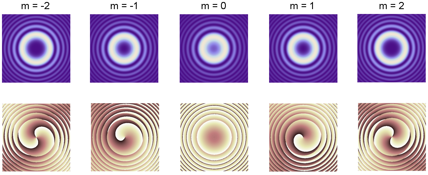
Figure 6: HyG beam intensity (upper row) and phase (lower row) transverse profiles ($y$-coordinate versus $x$-coordinate) for $\gamma=1$.

3.4 Hypergeometric-Gaussian beams

Taking into consideration the possibility of using complex parameters, we can set $a=i/2$, $b=0$, $\mu\left(\zeta\right)=\sqrt{\zeta\left(\zeta+i\right)}$ and $\phi\left(\zeta\right)=-\zeta$:

$$i\frac{\partial u_{HG}\left(r,\zeta\right)}{\partial\zeta}=\frac{1}{4\mu^{2}\left(\zeta\right)}\left[\frac{\partial^{2}}{\partial r^{2}}+\frac{1}{r}\frac{\partial}{\partial r}-2\left(r\frac{\partial}{\partial r}+1\right)-\frac{m^{2}}{r^{2}}\right]u_{HG}\left(r,\zeta\right).$$ (44)

Let us suppose the function $u_{HG}$ to be factorized as:

$$u_{HG}\left(r,\zeta\right)\propto r^{\left|m\right|}Z_{HG}\left(\zeta\right)HG\left(r^{2}\right),$$ (45)

then (44) reduces to:

$$r^{2}HG^{{}^{\prime\prime}}+\left[\left(\left|m\right|+1\right)-r^{2}\right]HG^{{}^{\prime}}-\left[\frac{\left|m\right|+1}{2}+i\frac{\mu^{2}}{Z_{HG}}\frac{dZ_{HG}}{d\zeta}\right]HG=0.$$ (46)

Following the usual procedure, it is required that:

$$i\frac{\mu^{2}\left(\zeta\right)}{Z_{HG}\left(\zeta\right)}\frac{dZ_{HG}\left(\zeta\right)}{d\zeta}=-\frac{\eta+\left|m\right|+1}{2},$$ (47)

where $\eta\in\mathbb{R}$. A quick integration gives:

$$Z_{HG}\left(\zeta\right)=\left(\frac{\zeta}{\zeta+i}\right)^{\frac{\eta+\left|m\right|+1}{2}},$$ (48)

whereas the Kummer equation [78] arises from (46):

$$r^{2}HG^{{}^{\prime\prime}}\left(r^{2}\right)+\left[\left(\left|m\right|+1\right)-r^{2}\right]HG^{{}^{\prime}}\left(r^{2}\right)+\frac{\eta}{2}HG\left(r^{2}\right)=0,$$ (49)

$$HG\left(r^{2}\right)={}_{1}F_{1}\left[-\frac{\eta}{2},\left|m\right|+1;\,r^{2}\right].$$ (50)

Expression (15) leads to:

$$f_{m}^{HG}\left(\rho,\varphi,z;\eta\right) = C_{m}^{HG}\left(\eta\right)\left(\frac{\rho}{w_{0}}\right)^{\left|m\right|}\left(\frac{z}{z_{R}}\right)^{\frac{\eta}{2}}\left(\frac{z}{z_{R}}+i\right)^{-\left(1+\left|m\right|+\frac{\eta}{2}\right)}\exp\left(im\varphi\right)$$ (51)

$$\times {}_{1}F_{1}\left[-\frac{\eta}{2},\left|m\right|+1;\,\frac{k\rho^{2}}{2z\left(\frac{z}{z_{R}}+i\right)}\right]\exp\left[-i\frac{\rho^{2}}{w_{0}^{2}\left(\frac{z}{z_{R}}+i\right)}\right].$$

The modes represented by $\Psi_{m}^{HG}\left(\rho,\varphi,z,t;\eta\right)=f_{m}^{HG}\left(\rho,\varphi,z;\eta\right)\mathrm{e}^{-ikz+i\omega t}$ constitute the family of the hypergeometric-Gaussian (HyGG) beams, an overcomplete set of non-orthogonal paraxial OAM solutions of the scalar wave equation [116]. It can be proven that these configurations carry a finite power (and therefore can be experimentally approximated) as long as the condition $\eta\geq-\left|m\right|$ is satisfied.

The HyGG beams are not shape-invariant modes under free propagation; as far as the asymptotic behavior is concerned, the radius of the primary maximum of their intensity profile follows the same law as the LG case for $m\neq 0$, namely $\rho_{max}^{HG}\left(z\right)\propto z$, which implies the usual decay of the intensity maximum at large distances, $I_{max}^{HG}\left(z\right)=\left|f_{m}^{HG}\left[\rho_{max}^{HG}\left(z\right),\varphi,z;\eta\right]\right|^{2}\propto z^{-2}$. Also the asymptotic evolution of the intensity at fixed $\rho=\bar{\rho}$ is found to be $I_{HG}\left(z\right)\propto z^{-2\left|m\right|-2}$, as for the LG beams.

3.5 Hypergeometric-Gaussian beams of the second kind

Another interesting family of cylindrical modes is found by choosing $a=-i/2$, $b=0$, $\mu\left(\zeta\right)=\sqrt{1-i\zeta}$ and $\phi\left(\zeta\right)=0$. In this case, equation (20) reads:

$$i\frac{\partial u_{HG_{II}}}{\partial\zeta}=\frac{1}{4\mu^{2}}\left[\frac{\partial^{2}}{\partial r^{2}}+\frac{1}{r}\frac{\partial}{\partial r}+2\left(r\frac{\partial}{\partial r}+1\right)-\frac{m^{2}}{r^{2}}\right]u_{HG_{II}}.$$ (52)

Let us suppose:

$$u_{HG_{II}}\left(r,\zeta\right)\propto r^{\left|m\right|}Z_{HG_{II}}\left(\zeta\right)\exp\left(-r^{2}\right)HG_{II}\left(r^{2}\right),$$ (53)

which implies:

$$r^{2}HG_{II}^{{}^{\prime\prime}}+\left[\left(\left|m\right|+1\right)-r^{2}\right]HG_{II}^{{}^{\prime}}-\left[\frac{\left|m\right|+1}{2}+i\frac{\mu^{2}}{Z_{HG_{II}}}\frac{dZ_{HG_{II}}}{d\zeta}\right]HG_{II}=0.$$ (54)

Let now:

$$i\frac{\mu^{2}\left(\zeta\right)}{Z_{HG_{II}}\left(\zeta\right)}\frac{dZ_{HG_{II}}\left(\zeta\right)}{d\zeta}=-\frac{\eta+\left|m\right|+1}{2},$$ (55)

whose solution is given by:

$$Z_{HG_{II}}\left(\zeta\right)=\left(1-i\zeta\right)^{-\frac{\eta+\left|m\right|+1}{2}}.$$ (56)

Equation (54) has the same form as (46), thus $HG_{II}\left(r^{2}\right)=HG\left(r^{2}\right)$, expression (50). Finally:

$$f_{m}^{HG_{II}}\left(\rho,\varphi,z;\eta\right) \!\!=\!\! C_{m}^{HG_{II}}\left(\eta\right)\left(\frac{\rho}{w_{0}}\right)^{\left|m\right|}\left(1-i\frac{z}{z_{R}}\right)^{-\left(1+\left|m\right|+\frac{\eta}{2}\right)}\exp\left(im\varphi\right)$$ (57)

$$\!\!\times\!\! {}_{1}F_{1}\left[-\frac{\eta}{2},\left|m\right|+1;\,\frac{\rho^{2}}{w_{0}^{2}\left(1-i\frac{z}{z_{R}}\right)}\right]\exp\left[-\frac{\rho^{2}}{w_{0}^{2}\left(1-i\frac{z}{z_{R}}\right)}\right].$$

Paraxial modes of the kind $\varPsi_{m}^{HG_{II}}\left(\rho,\varphi,z,t;\eta\right)=f_{m}^{HG_{II}}\left(\rho,\varphi,z;\eta\right)\mathrm{e}^{-ikz+i\omega t}$ are known as hypergeometric-Gaussian type-II (HyGG-II) beams and, like the HyGG modes, represent an overcomplete set of non-orthogonal OAM solutions of the Helmholtz equation which are square-integrable for $\eta\geq-\left|m\right|$, condition under which they carry a finite amount of energy [115].

The HyGG-II beams are not shape-invariant modes under free propagation (see Figure 7). Following the standard convention, where a propagation term of the form $\exp\left(ikz-i\omega t\right)$ is considered, inducing a change of sign in the $z$-derivative in (13), the function $\mu\left(\zeta\right)$ has the form $\sqrt{1+i\zeta}$ and equation (57) changes accordingly.

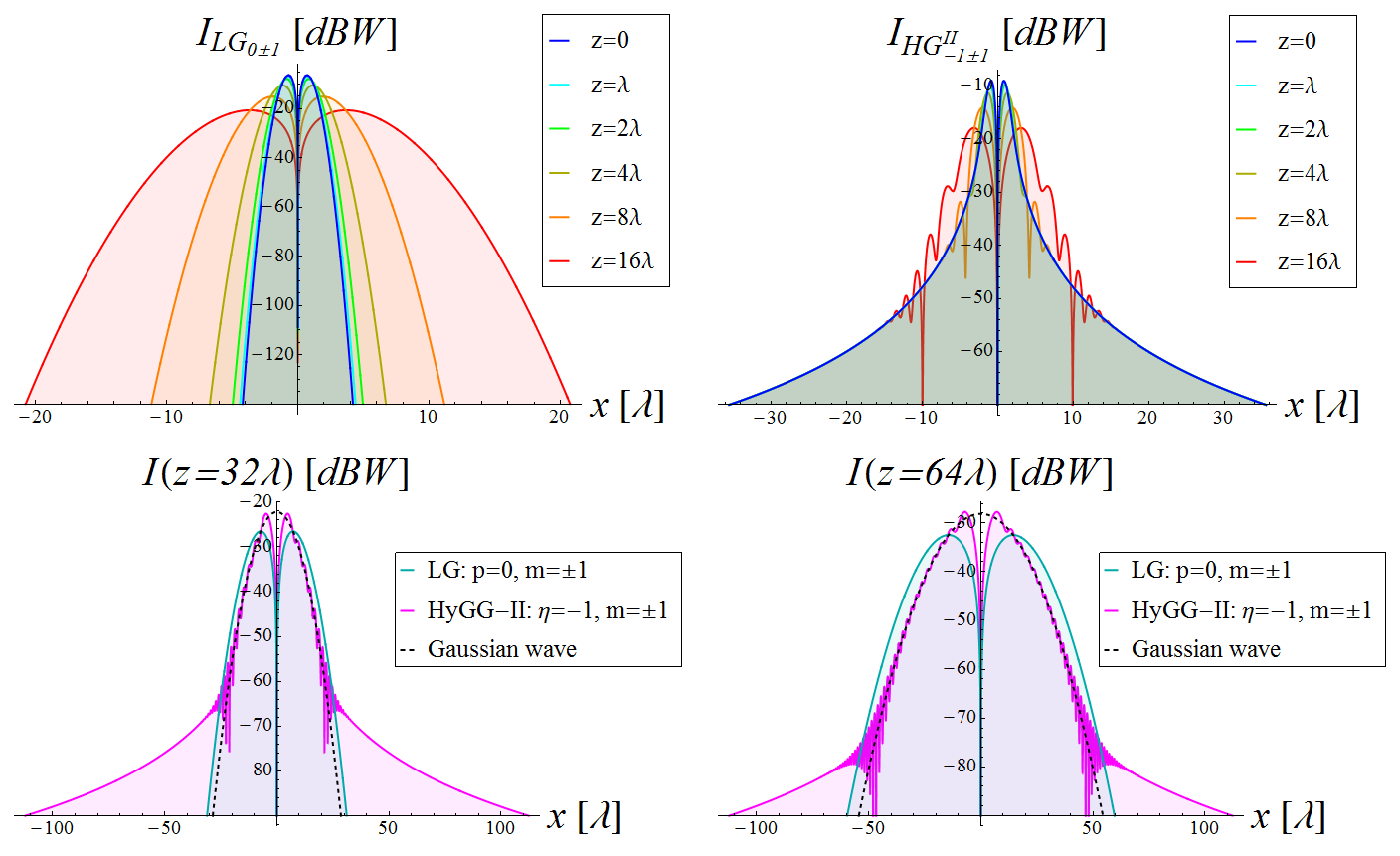
Figure 7: Comparison between the power profiles (per unit square meter) of a LG beam and of a HyGG-II beam evaluated in $y=0$, for $w_{0}=\lambda$.

Despite their name, resembling the previous family, the HyGG-II beams show significant differences with respect to the other known solutions. First, the radius of their primary intensity maximum increases with $z$ according to two possible asymptotic behaviors, depending on the choice of the $\eta$ and $m$ indices: when $\eta=-\left|m\right|\neq 0$, a square root law is found, $\rho_{max}^{HG_{II}}\left(z\right)\propto\sqrt{z}$, whereas the usual linear behavior $\rho_{max}^{HG_{II}}\left(z\right)\propto z$ is quickly reached by all the configurations in which $\eta>0$ for every $m$ or $\eta\geq 0$ for $m\neq 0$ (the doughnut-shaped asymptotic profile is always present, except for the standard Gaussian wave $\eta=m=0$). It is fundamental to understand that the square root divergence of the primary intensity maximum relative to the HyGG-II modes in the first subclass does not apply to the beam profile in its entirety, as can be inferred from the comparison reported in Figure 7.

Since the $\eta$ parameter must be greater than or equal to $-\left|m\right|$ in order to ensure square-integrability, the whole range $-\left|m\right|<\eta<0$ where $m$ is not zero can be explored: in this region, as a consequence of the very rippled and variable field pattern, the primary intensity maximum oscillates at different radii in the beam profile and it evolves alternating between the two possible above described laws as a function of the propagation coordinate, asymptotically stabilizing to the linear evolution in $z$ (see Figure 8).

In order to establish the decay law of the primary intensity maximum, the two asymptotic cases must be considered separately. If $\eta=-\left|m\right|\neq 0$, the argument of the Kummer function in (57), as well as that of the exponential, tends to a constant value for large $z$ and so we immediately get $I_{max}^{HG_{II}}\left(z\right)=\left|f_{m}^{HG_{II}}\left[\rho_{max}^{HG_{II}}\left(z\right),\varphi,z;-\left|m\right|\right]\right|^{2}\propto z^{-2}$. On the other hand, when $\eta>-\left|m\right|$ a useful asymptotic expansion of the Kummer function can be employed [78]:

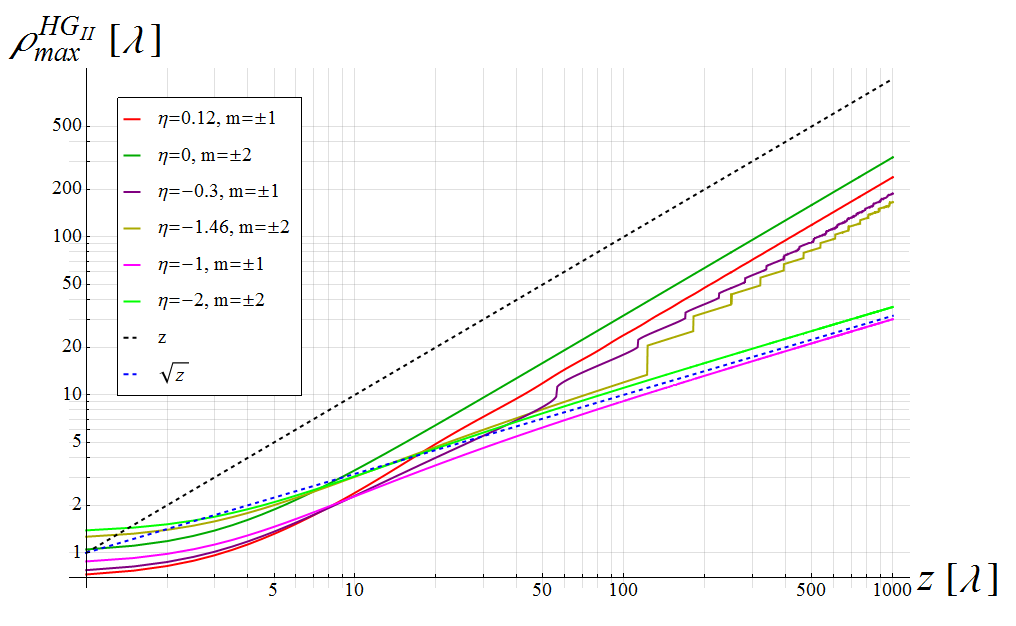
Figure 8: Evolution of the radial coordinate of the principal intensity maximum of some HyGG-II beams as a function of $z$, for $w_{0}=\lambda$. Note that for $-\left|m\right|<\eta<0$ unstable maxima of the intensity profile with different evolution in $z$ are competing in a certain range of the propagation coordinate; since the plot only captures the principal maximum at each $z$, this results in a stair-like behavior.

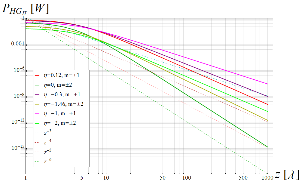
Figure 9: Evolution of the integral of the intensity of some HyGG-II beams over a centered circular region with radius $w_{0}$ as a function of $z$, for $w_{0}=\lambda$.

$${}_{1}F_{1}\left(a,b;\,x\right)\approx\Gamma\left(b\right)\left[\frac{\exp\left(x\right)x^{a-b}}{\Gamma\left(a\right)}+\frac{\left(-x\right)^{-a}}{\Gamma\left(b-a\right)}\right],$$ (58)

which applies for large $\left|x\right|$. Remembering that now $\rho_{max}^{HG_{II}}\left(z\right)\propto z$, the local far-field intensity reduces to:

$$I_{max}^{HG_{II}}\left(z\right)\propto z^{2\left|m\right|}z^{-\left(2+2\left|m\right|+\eta\right)}\left|\frac{\mathrm{e}^{i\pi\frac{z}{\lambda}}\left(i\pi\frac{z}{\lambda}\right)^{-\frac{\eta}{2}-\left|m\right|-1}}{\Gamma\left(-\frac{\eta}{2}\right)}+\frac{\left(-i\pi\frac{z}{\lambda}\right)^{\frac{\eta}{2}}}{\Gamma\left(\left|m\right|+1+\frac{\eta}{2}\right)}\right|^{2},$$ (59)

where expression (58) was used. Since the second term in the sum under square modulus dominates over the first at large $z$, this enables us to obtain $I_{max}^{HG_{II}}\left(z\right)\propto z^{-2}$, which then holds true for every $\eta\geq-\left|m\right|$.

Finally, at fixed radial coordinate and large enough $z$, it is easy to prove that $I_{HG_{II}}\left(z\right)\propto z^{-\eta-2\left|m\right|-2}$, which also describes the power decay in a central region of the beam as a function of the propagation distance, displayed in Figure 9. Of special interest is the case $\eta=-\left|m\right|$, corresponding to the best possible evolution, $z^{-\left|m\right|-2}$.

3.6 Bessel-Gaussian beams

In Section 3.1 it was said that BBs are not square-integrable; however, there exist paraxial solutions of the Helmholtz equation which consists in non-diffracting modes modulated by a Gaussian envelope. Such beams are known as Helmholtz-Gaussian (HzG) waves [114]. Although these modulated solutions lose the divergence-free behavior, they present the advantage of being square-integrable and therefore admit physical realization. In the case of a Bessel configuration, the corresponding HzG solutions are given by the Bessel-Gaussian (BG) beams $\varPsi_{m}^{BG}\left(\rho,\varphi,z,t;k_{\rho}\right)=f_{m}^{BG}\left(\rho,\varphi,z;k_{\rho}\right)\mathrm{e}^{-ikz+i\omega t}$, achievable from expressions (15) and (20) through the choice $a=-i$, $b=1$, $\mu\left(\zeta\right)=1-i\zeta$ and $\phi\left(\zeta\right)=\zeta$, which leads to:

$$i\frac{\partial u_{BG}}{\partial\zeta}=\frac{1}{4\mu^{2}}\left[\frac{\partial^{2}}{\partial r^{2}}+\frac{1}{r}\frac{\partial}{\partial r}+4\left(r\frac{\partial}{\partial r}+1\right)-\frac{m^{2}}{r^{2}}+4r^{2}\right]u_{BG}.$$ (60)

With reference to Section 3.1:

$$u_{BG}\left(r,\zeta\right)\propto\exp\left(-r^{2}\right)BG\left(r\right)\exp\left(i\frac{w_{0}^{2}k_{\rho}^{2}\zeta}{4\mu\left(\zeta\right)}\right).$$ (61)

Equation (60) is easily reduced to the following:

$$r^{2}\frac{d^{2}BG\left(r\right)}{dr^{2}}+r\frac{dBG\left(r\right)}{dr}+\left(r^{2}w{}_{0}^{2}k_{\rho}^{2}-m^{2}\right)BG\left(r\right)=0,$$ (62)

corresponding to Bessel equation in the variable $\left(\rho/\mu\right)$. Then, from (15):

$$f_{m}^{BG}\left(\rho,\varphi,z;k_{\rho}\right) = \frac{C_{m}^{BG}\left(k_{\rho}\right)}{1-i\frac{z}{z_{R}}}J_{\left|m\right|}\left(\frac{k_{\rho}\rho}{1-i\frac{z}{z_{R}}}\right)\exp\left(im\varphi\right)$$ (63)

$$\times \exp\left[-\frac{\rho^{2}}{w_{0}^{2}\left(1-i\frac{z}{z_{R}}\right)}+i\frac{k_{\rho}^{2}z}{2k\left(1-i\frac{z}{z_{R}}\right)}\right].$$

Once again, due to the convention employed for the propagation term, equation (63) is not of the form usually reported in the literature: in order to obtain the standard expression, the whole procedure presented in Section 3 should be repeated starting from the assumption $\psi\left(\rho,\varphi,z\right)=f\left(\rho,\varphi,z\right)\mathrm{e}^{ikz}$.

The intensity distribution of the BG beams is strongly related to the value of the transverse momentum $k_{\rho}$ as well as to the beam waist $w_{0}$ of the Gaussian envelope [111]. The evolution of the radius of the maximum intensity follows the asymptotic law $\rho_{max}^{BG}\left(z\right)\propto z$ (for certain choices of the $k_{\rho}$ parameter a doughnut-shaped profile is also generated when $m=0$, instead of the usual maximum at $\rho=0$). At large distances, $I_{max}^{BG}\left(z\right)=\left|f_{m}^{BG}\left[\rho_{max}^{BG}\left(z\right),\varphi,z;k_{\rho}\right]\right|^{2}\propto z^{-2}$. By exploiting the well-known relation [78]:

$$J_{\alpha}(x)\approx\frac{1}{\Gamma\left(\alpha+1\right)}\left(\frac{x}{2}\right)^{\alpha},$$ (64)

which holds for small $\left|x\right|$, it is possible to infer the decay law of the BG beams intensity in $\rho=\bar{\rho}$ at large $z$: $I_{BG}\left(z\right)\propto z^{-2\left|m\right|-2}$.

To conclude the section, a comparison of the longitudinal intensity profiles of some representative solutions belonging to each of the above described paraxial families is reported in Figure 10. As it can be noticed, the energy distribution of these scalar waves as a function of the propagation coordinate varies considerably from beam to beam.

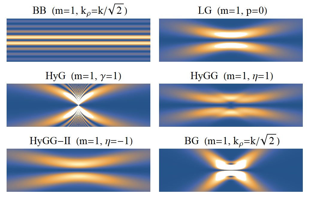
Figure 10: Comparison of the longitudinal intensity profiles ($x$-coordinate versus $z$-coordinate) of some paraxial beams for $w_{0}=\lambda$.

4 Vortex solutions of the vector wave equation

As shown in the two previous sections, exact and paraxial solutions of the scalar wave equation which are eigenfunctions of the $\hat{J}_{z}$ operator can be easily derived by means of standard mathematical techniques; indeed, such scalar OAM solutions have been deeply explored in the literature. However, an electromagnetic field can hardly be described in terms of a pure scalar function of space and time, since only a full vector treatment allows to take into account the presence of complex polarization structures. Complete solutions of the vector wave equation that can be directly applied to boundary-value problems in electromagnetism have been derived for certain separable systems of cylindrical coordinates and for spherical coordinates: in this context, the electromagnetic field can be resolved into two partial fields, each derivable from a function satisfying the scalar wave equation [74, 131].

Within any closed domain of a homogeneous and isotropic medium with zero conductivity and free-charge density, all vectors characterizing the electromagnetic field satisfy:

$$\nabla^{2}\boldsymbol{\Psi}-\epsilon\mu\frac{\partial^{2}\boldsymbol{\Psi}}{\partial t^{2}}=0,$$ (65)

being $\epsilon$ and $\mu$ the inductive capacities of the medium. On using the following relation:

$$\nabla^{2}\boldsymbol{\Psi}=\nabla\left(\nabla\cdot\boldsymbol{\Psi}\right)-\nabla\times\nabla\times\boldsymbol{\Psi}$$ (66)

and assuming a time-harmonic dependence of the form $\exp\left(i\omega t\right)$, equation (65) becomes:

$$\nabla\left(\nabla\cdot\boldsymbol{\psi}\right)-\nabla\times\nabla\times\boldsymbol{\psi}+k^{2}\boldsymbol{\psi}=0,$$ (67)

with $k=\epsilon\mu\omega^{2}$. Equation (67) represents the vector analog of (4). As emphasized by Julius A. Stratton in [131], equation (67) can always be replaced by a system of three scalar equations, but it is only when $\boldsymbol{\psi}$ is expressed in rectangular components that three independent scalar equations are obtained:

$$\nabla^{2}\psi_{x}+k^{2}\psi_{x}=0;\quad\nabla^{2}\psi_{y}+k^{2}\psi_{y}=0;\quad\nabla^{2}\psi_{z}+k^{2}\psi_{z}=0.$$ (68)

The Laplacian in (68) can of course be written in different coordinate systems, but the vector character of the original equation is inevitably lost. Three independent vector solutions of (67) can instead be built as follows:

$$\mathbf{M}=\nabla\times\mathbf{C}g;\quad\mathbf{N}=\frac{1}{k}\nabla\times\mathbf{M};\quad\mathbf{L}=\nabla g,$$ (69)

being $g=g\left(x_{1},x_{2},x_{3}\right)$ a scalar function satisfying (4) and $\mathbf{C}$ a unit norm constant vector. The three vector functions above possess several interesting properties: $\mathbf{M}=\mathbf{L}\times\mathbf{C}=k^{-1}\nabla\times\mathbf{N}$, $\mathbf{L}\cdot\mathbf{M}=0$, $\nabla\times\mathbf{L}=0$, $\nabla\cdot\mathbf{L}=-k^{2}g$; moreover, it is easy to prove that both $\mathbf{M}$ and $\mathbf{N}$ are solenoidal and, owing to this and to the fact of being each proportional to the curl of the other, can be employed to represent the electric and magnetic fields.

Since a decomposition of any arbitrary vector wavefunction in terms of (69) is completely general, families of orthogonal vector solutions of the wave equation (65) are derived via (69) from sets of solutions of the scalar wave equation (3) in the various coordinate systems. Also the field polarization is now being considered and care must be taken to properly describe the action of the rotation group generators on the whole vector field.

As can be shown by expanding to first order an infinitesimal rotation about the $z$-axis (see B), the complete form of the $\hat{J}_{z}$ operator for vector fields is provided by:

$$i\hat{J}_{z}=-i\frac{\partial}{\partial\varphi}+iS_{z},$$ (70)

where $S_{z}$ corresponds to the third SO(3) generator in three-dimensional matrix representation. When the vector field is resolved into its Cartesian components, the explicit expression for $S_{z}$ is given by $J_{3}$ in (2) and equation (70) reduces to its more common form [132]:

$$i\hat{J}_{z}=-i\left(x\frac{\partial}{\partial y}-y\frac{\partial}{\partial x}\right)+\left[\begin{array}[]{ccc}0&-i&0\\ i&0&0\\ 0&0&0\end{array}\right].$$ (71)

Let $\left\{g_{m}\right\}=\left\{\varPhi_{m}\left(\varphi\right)u\left(x_{1},x_{3}\right)\right\}$ be a set of OAM scalar functions derived according to Section 2. A general vector solution of (67) can be constructed from $\left\{g_{m}\right\}$ via the superposition:

$$\boldsymbol{\psi}=\frac{i}{\omega}\sum_{m}\left(a_{m}\mathbf{M}_{m}+b_{m}\mathbf{N}_{m}+c_{m}\mathbf{L}_{m}\right),$$ (72)

where $a_{m}$, $b_{m}$ and $c_{m}$ represent suitable expansion coefficients and the vector fields in the set $\left\{\mathbf{M}_{m},\mathbf{N}_{m},\mathbf{L}_{m}\right\}$ are provided by (69) with $g=g_{m}$. Therefore, the transformation of $\mathbf{\boldsymbol{\psi}}$ under an infinitesimal rotation about the $z$-axis leads back to the action of the $\hat{J}_{z}$ operator on each basis function. In all the five separable coordinate systems for which the $\varphi$-coordinate exists, the following relations hold:

$$i\hat{J}_{z}\mathbf{M}_{m}=m\mathbf{M}_{m};\quad i\hat{J}_{z}\mathbf{N}_{m}=m\mathbf{N}_{m};\quad i\hat{J}_{z}\mathbf{L}_{m}=m\mathbf{L}_{m},$$ (73)

as explicitly shown in B. The importance of this last result lies in the fact that it is the only requirement of separability of the scalar Helmholtz equation which ensures the vector fields $\left\{\mathbf{M}_{m},\mathbf{N}_{m},\mathbf{L}_{m}\right\}$ built from the OAM set $\left\{g_{m}\right\}$ to be eigenfunctions of the $\hat{J}_{z}$ operator.

From (69), (70) and (73) we understand that the so-derived eigenfunctions cannot be simply considered as vector OAM waves, since their structure is in general more complex, also involving polarization and thus a SAM contribution. Furthermore, for all the three eigenfunctions in (73), it is the vector field components which present the characteristic vortex term $\varPhi_{m}\left(\varphi\right)$, meaning that the phase evolution around the $z$-axis is accompanied by the evolution of the state of polarization. Such eigenfunctions are then named vector vortex beams (VVBs), bearing in mind that in this case the on-axis phase singularity is no longer exclusive and also polarization singularities may be present (see, for instance, [133, 134, 135, 136, 92] and references therein). The above described approach undoubtedly provides a rigorous method for understanding how the VVBs definition can be traced back to general symmetry arguments.

In order to give some instructive examples, let us suppose that the vector potential $\mathbf{A}$ can be represented by an expansion in characteristic vector functions, as in (72). The electric field $\mathbf{E}$ in the Lorentz gauge is then expressed by:

$$\mathbf{E}=-\sum_{m}\left(a_{m}\mathbf{M}_{m}+b_{m}\mathbf{N}_{m}\right),$$ (74)

the usual time-harmonic term $\exp\left(i\omega t\right)$ being implied. Considering a circular cylindrical coordinate system, for which the natural OAM scalar field basis $\left\{g_{m}\right\}$ is provided by BBs, and choosing the $z$-directed unit vector as $\mathbf{C}$ in (69), we get:

$$\mathbf{M}_{m}=\frac{k_{\rho}}{2}\left[i\left(J_{m-1}+J_{m+1}\right)\mathbf{u}_{\rho}-\left(J_{m-1}-J_{m+1}\right)\mathbf{u}_{\varphi}\right]\mathrm{e}^{-ik_{z}z+im\varphi};$$ (75)

$$\mathbf{N}_{m} = \frac{k_{\rho}}{2k}\left[-ik_{z}\left(J_{m-1}-J_{m+1}\right)\mathbf{u}_{\rho}+k_{z}\left(J_{m-1}+J_{m+1}\right)\mathbf{u}_{\varphi}\right.$$ (76)

$$+ \left.2k_{\rho}J_{m}\mathbf{u}_{z}\right]\exp\left(-ik_{z}z+im\varphi\right),$$

where all Bessel functions have argument $\left(k_{\rho}\rho\right)$, $\left\{\mathbf{u}_{\rho},\mathbf{u}_{\varphi},\mathbf{u}_{z}\right\}$ represent the cylindrical system unit vectors and (10) has been employed together with some known properties of Bessel functions under the assumption $m\geq 0$, for convenience.

In Figure 11, the norm and polarization plots of (75) are reported for some values of $m$, revealing two apparent deviations from the conventional OAM patterns: when $m=0$, a null is present instead of the usual on-axis intensity maximum, whereas for $m=1$ the central null is replaced by a maximum.

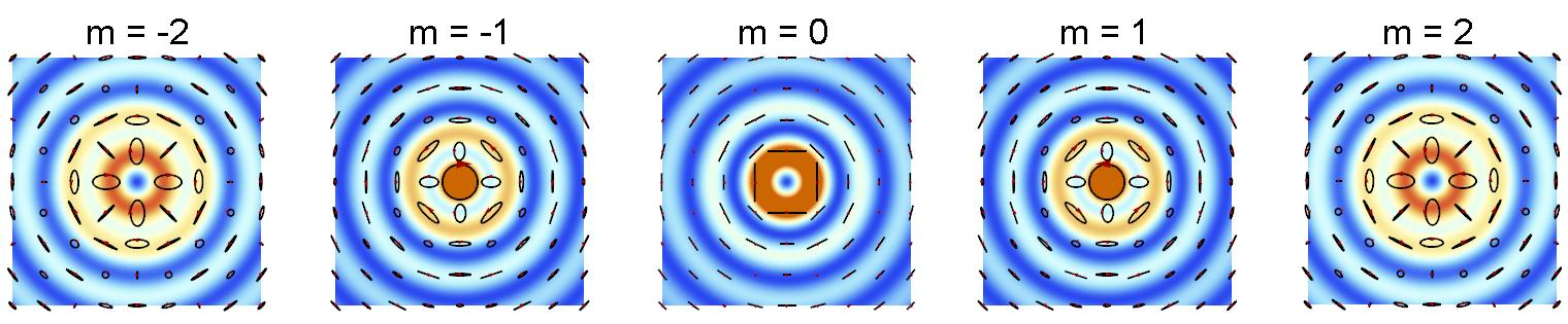
Figure 11: Norm and polarization plots ($y$-coordinate versus $x$-coordinate) of the function $\mathbf{M}_{m}$ defined in (75) for $k_{\rho}=k/\sqrt{2}$.

Both deviations are attributable to the mixing of spatial and polarization contributions, which also affects all the other modes, as evidenced by the circumstance that additional factors $\mathrm{e}^{\pm i\varphi}$ appear once (75) is rewritten in terms of the Cartesian unit vectors. It should be noted that the presence of the on-axis intensity null in the $m=0$ case results from a polarization singularity known as V point in singular optics [135].

In [137], Karen Volke-Sepúlveda et al. have shown that equations (74), (75) and (76) make it possible to describe a wide variety of vector solutions in different polarization states. For instance, a radially or azimuthally polarized beam can be obtained by setting $a_{m}=0$ and $b_{m}=i\delta_{m0}E_{0}k/\left(k_{\rho}k_{z}\right)$ or $a_{m}=-\delta_{m0}E_{0}/k_{\rho}$ and $b_{m}=0$ in (74), respectively; here $E_{0}$ represents a constant proportional to the square root of the beam power and with electric field units. Such peculiar vector waves with circular symmetric structure can be seen as free-space transverse magnetic (TM) and transverse electric (TE) modes, as can be deduced from their electric field expressions:

$$\mathbf{E}_{R}=E_{0}\left[J_{1}\left(k_{\rho}\rho\right)\mathbf{u}_{\rho}-i\left(\frac{k_{\rho}}{k_{z}}\right)J_{0}\left(k_{\rho}\rho\right)\mathbf{u}_{z}\right]\exp\left(-ik_{z}z+i\omega t\right);$$ (77)

$$\mathbf{E}_{A}=E_{0}\left[J_{1}\left(k_{\rho}\rho\right)\mathbf{u}_{\varphi}\right]\exp\left(-ik_{z}z+i\omega t\right),$$ (78)

where the subscripts $R$ and $A$ stand for radial and azimuthal, respectively, and the time dependence is now explicitly written. Both (77) and (78) are eigenfunctions of the $\hat{J}_{z}$ operator with eigenvalue $m=0$, by construction.

Following the approach presented in [137], right-handed and left-handed circular polarized modes are easily derived from $b_{m}=\mp a_{m}k/k_{z}$ upon proper choice of the $a_{m}$ coefficients:

$$\mathbf{E}_{\pm}=E_{0}\left[J_{m}\left(k_{\rho}\rho\right)\left(i\mathbf{u}_{x}\mp\mathbf{u}_{y}\right)\mp\left(\frac{k_{\rho}}{k_{z}}\right)\mathrm{e}^{\pm i\varphi}J_{m\pm 1}\left(k_{\rho}\rho\right)\mathbf{u}_{z}\right]\mathrm{e}^{-ik_{z}z+im\varphi+i\omega t},$$ (79)

being $\left\{\mathbf{u}_{x},\mathbf{u}_{y},\mathbf{u}_{z}\right\}$ the Cartesian unit vectors. In particular, since equation (79) is obtained from the $\left(m\pm 1\right)$ term of (74), we find:

$$i\hat{J}_{z}\mathbf{E}_{\pm}=\left(m\pm 1\right)\mathbf{E}_{\pm},$$ (80)

as can be inferred from (73) or explicitly verified using (71). Whereas the two orthogonal $x$-polarized and $y$-polarized states are simple superpositions of the right-circular and left-circular ones, the most general field is given in terms of the Jones vector Cartesian components $\alpha$ and $\beta$ [5]:

$$\mathbf{E} = E_{0}\left\{\left(\frac{-ik_{\rho}}{2k_{z}}\right)\left[\left(\alpha+i\beta\right)\mathrm{e}^{-i\varphi}J_{m-1}\left(k_{\rho}\rho\right)-\left(\alpha-i\beta\right)\mathrm{e}^{i\varphi}J_{m+1}\left(k_{\rho}\rho\right)\right]\mathbf{u}_{z}\right.$$ (81)

$$+ \left.\left[\alpha\mathbf{u}_{x}+\beta\mathbf{u}_{y}\right]J_{m}\left(k_{\rho}\rho\right)\frac{}{}\right\}\exp\left(-ik_{z}z+im\varphi+i\omega t\right).$$

For $\beta=\pm i\alpha$, equation (81) leads back to (79). Any other choice of the polarization parameters $\alpha$ and $\beta$ in (81) does not give rise to an eigenvector of the $\hat{J}_{z}$ operator, as evidenced by the fact that the circular symmetry of both the beam energy and polarization is broken (see Figure 12). The angular momentum density for the various cylindrical solutions described above has been rigorously calculated in [137], showing that its distribution is indeed not radially symmetric in the case of linearly polarized BBs. On the other hand, the presence of the ratio $\left(k_{\rho}/k_{z}\right)$ in all previous formulas makes it possible to extend the analysis to the paraxial regime $k_{\rho}\ll k_{z}$, with which most of the literature is concerned. Under this approximation, the electric field $\mathbf{E}$ in (81) is found to be eigenvector of $-i\partial/\partial\varphi$, the orbital component of $i\hat{J}_{z}$, and the circular symmetry of the solution norm is restored, as it is shown in Figure 12. Despite the analytic expressions for paraxial VVBs may be obtained more practically by non-separable combinations of spatial and polarization modes [48], the above derivation could be in some circumstances preferable.

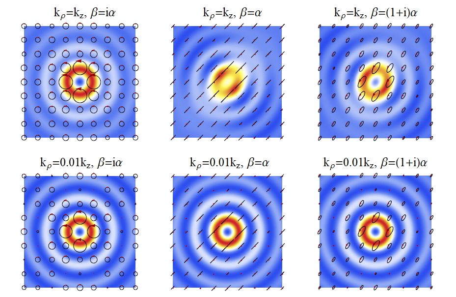
Figure 12: Norm and polarization plots ($y$-coordinate versus $x$-coordinate) of the electric field $\mathbf{E}$ in (81) for some nonparaxial (upper row) and paraxial (lower row) solutions with $m=1$.

Finally, among the various paraxial and non-paraxial VVBs, vector beams presenting cylindrical symmetric states of polarization, often known as cylindrical vector (CV) beams or vortices, have been extensively analyzed due to their interesting properties such as the tighter waist upon focusing (a thorough review of the applications can be found in [138]).

5 Conclusions

In this work, an in-depth overview on the exact and paraxial vortex solutions of the homogeneous wave equation has been presented. These solutions have been interpreted as eigenstates of the $\hat{J}_{z}$ operator, leading to a mixture of polarization and spatial modes in the case of a general vector vortex wave.

Whereas a scalar approach is often convenient to describe the transverse free-space modes of linearly polarized laser radiation in optics, the same does not hold for the radio frequency domain, where a full vector treatment is usually mandatory. In neither cases could the homogeneous wave equation probably be sufficient for the most realistic modeling of the OAM waveforms generated experimentally by means of resonators and antennas, for which only the complete Maxwell equations with real or equivalent source terms can ideally provide the highest level of accuracy. Nevertheless, it is unquestionably true that the homogeneous Helmholtz equation still represents the most affordable way for describing specific free-space solutions as well as for providing general basis sets to expand any arbitrary waveform. For instance, the scalar and vector OAM solutions analyzed in this paper could be easily interpreted as free-space generalizations of resonator and waveguide eigenmodes that are usually found in both laser theory and electromagnetics handbooks. The intensity, phase, polarization and propagation properties of such free-space beams are therefore considered as ideal reference models or, alternatively, as targets to be reproduced experimentally up to a certain degree of approximation via proper synthesis methods. Since many of the exact vortex solutions possess infinite transverse extension, are divergence-free and carry infinite energy, paraxial OAM waves with Gaussian envelope or truncated forms which take into account diffraction and finite-size effects must be preferred in order to ensure a more realistic description.

The main ideas and results of this work were carried out during my PhD in physics at the University of Torino. Among the various people to whom I am indebted, I would like to especially thank Prof. Roberto Tateo, Prof. Paolo Gambino and Prof. Miguel Onorato, from the Department of Physics, Dr. Rossella Gaffoglio, Prof. Francesco Andriulli and Prof. Giuseppe Vecchi, from the Polytechnic University of Torino, Dr. Assunta De Vita and Eng. Bruno Sacco, from the Centre for Research and Technological Innovation, RAI Radiotelevisione Italiana.

Appendix A Vortex solutions in different coordinate systems

A.1 Spherical coordinates

When expressed in a spherical coordinate system, the scalar Helmholtz equation (4) reads:

$$\frac{1}{r}\frac{\partial^{2}\left(r\psi\right)}{\partial r^{2}}+\frac{1}{r^{2}\sin\theta}\frac{\partial}{\partial\theta}\left(\sin\theta\frac{\partial\psi}{\partial\theta}\right)+\frac{1}{r^{2}\sin^{2}\theta}\frac{\partial^{2}\psi}{\partial\phi^{2}}+k^{2}\psi=0.$$ (82)

This section is devoted to the search for spherical OAM solutions of the form:

$$\psi\left(r,\theta,\phi\right)=C\,\frac{\exp\left(-ikr+im\phi\right)}{r}R\left(r\right)\Theta\left(\theta\right),$$ (83)

where $R\left(r\right)$ and $\Theta\left(\theta\right)$ represent functions to be determined and $C$ is a constant. It is immediate to verify that, in order for (83) to satisfy equation (82), $\Theta$ cannot be constant. As a first step, for simplicity, it can be assumed that $R=1$, so that equation (82) reduces to:

$$\frac{d^{2}\Theta\left(\theta\right)}{d\theta^{2}}+\cot\theta\frac{d\Theta\left(\theta\right)}{d\theta}-m^{2}\left(\csc\theta\right)^{2}\Theta\left(\theta\right)=0,$$ (84)

provided that $r\neq 0$. By introducing the parametric coordinate $t=\tan\left(\theta/2\right)$, from which $\cos\theta=\frac{1-t^{2}}{1+t^{2}}$ and $\sin\theta=\frac{2t}{1+t^{2}}$ follow, we get:

$$\frac{d^{2}\Theta\left(t\right)}{dt^{2}}+\frac{1}{t}\frac{d\Theta\left(t\right)}{dt}-\frac{m^{2}}{t^{2}}\Theta\left(t\right)=0,$$ (85)

a Fuchsian ordinary differential equation with singularity in $t=0$. Since the roots of the corresponding indicial equation are $\pm\left|m\right|$, the two linearly independent solutions of (85) can be written in the following way:

$$\begin{cases}\Theta^{(1)}\left(t\right)=\sum_{k=0}^{\infty}c_{k}\,t^{k+\left|m\right|};\\ \Theta^{(2)}\left(t\right)=\sum_{k=0}^{\infty}d_{k}\,t^{k-\left|m\right|}+d\,\Theta^{(1)}\left(t\right)\log\left(t\right).\end{cases}$$ (86)

From substitution of the power series in (85) we easily find $k,\,d=0$, hence $\Theta^{(1)}\left(t\right)=t^{\left|m\right|}$ and $\Theta^{(2)}\left(t\right)=t^{-\left|m\right|}$, where only the first represents a regular solution in $t=0$. Then, expression (83) reduces to:

$$\psi\left(r,\theta,\phi\right)=C\,\frac{\exp\left(-ikr+im\phi\right)}{r}\left[\tan\left(\frac{\theta}{2}\right)\right]^{\left|m\right|},$$ (87)

which is not defined for $\theta=\pi$. A regularized version of the previous function over the whole sphere can be provided through the use of both $\Theta^{(1)}$ and $\Theta^{(2)}$, for instance:

$$\psi_{reg}\left(r,\theta,\phi\right)=C\,\frac{\exp\left(-ikr+im\phi\right)}{r}\begin{cases}\left[\tan\left(\frac{\theta}{2}\right)\right]^{\left|m\right|}&\mathrm{for}\,\theta\in\left[0,\frac{\pi}{2}\right];\\ \left[\tan\left(\frac{\theta}{2}\right)\right]^{-\left|m\right|}&\mathrm{for}\,\theta\in\left(\frac{\pi}{2},\pi\right].\end{cases}$$ (88)

OAM waves of the form (87) and (88) may be called “helico-polar” modes, as they possess helical wavefronts and show a very simple dependence on the polar angle $\theta$. It can be shown that these non-paraxial waves represent square-integrable solutions with respect to the spherical measure $\sin\theta d\theta d\phi$.

In order to prove that the well-known spherical multipoles correspond to generalizations of the above derived waves, the radial term $R\left(r\right)$ in (83) is now reintroduced. Equation (82) becomes:

$$-\frac{2ik}{r}\dot{R}\Theta+\frac{1}{r}\ddot{R}\Theta+\frac{\cot\theta}{r^{3}}R\dot{\Theta}+\frac{1}{r^{3}}R\ddot{\Theta}{\displaystyle-\frac{m^{2}\left(\csc\theta\right)^{2}}{r^{3}}R\Theta=0},$$ (89)

where the simplified notation $\dot{X}\left(x\right)=dX\left(x\right)/dx$ has been employed. Then, for $r\neq 0$ we find:

$$\begin{cases}\ddot{R}-2ik\dot{R}+\frac{L}{r^{2}}R=0;\\ \ddot{\Theta}+\cot\theta\dot{\Theta}-\left[m^{2}\left(\csc\theta\right)^{2}+L\right]\Theta=0,\end{cases}$$ (90)

being $L$ a constant term. To solve the first equation we set $R=\sqrt{r}\mathcal{R}\left(r\right)\mathrm{e}^{ikr}$, which leads to Bessel equation in $kr$:

$$r^{2}\mathcal{\ddot{R}}+r\mathcal{\dot{R}}+\left(k^{2}r^{2}+L-\frac{1}{4}\right)\mathcal{R}=0,$$ (91)

and therefore:

$$\begin{cases}R^{(1)}=\exp\left(ikr\right)\sqrt{r}\,J_{\frac{1}{2}\sqrt{1-4L}}\left(kr\right);\\ R^{(2)}=\exp\left(ikr\right)\sqrt{r}\,Y_{\frac{1}{2}\sqrt{1-4L}}\left(kr\right)\end{cases}$$ (92)

represent the two linearly independent radial solutions, given in terms of Bessel functions of the first and second kind, respectively. After performing the substitution $\cos\theta=t$, the second equation in (90) is easily reduced to:

$$\left(1-t^{2}\right)\frac{d^{2}\Theta\left(t\right)}{dt^{2}}-2t\frac{d\Theta\left(t\right)}{dt}-\left(L+\frac{m^{2}}{1-t^{2}}\right)\Theta\left(t\right)=0,$$ (93)

which admits solutions in terms of the generalized Legendre polynomials. Finally, by imposing the regularity of $\Theta$ at the boundary points, it can be proven that $L=-\ell\left(\ell+1\right)$ for an integer $\ell\geq\left|m\right|$ and equation (83) acquires the standard form:

$$\psi\left(r,\theta,\phi\right)=b_{\ell}\left(kr\right)Y_{\ell}^{m}\left(\theta,\phi\right),$$ (94)

where $b_{\ell}\left(kr\right)$ corresponds to a linear combination of the two independent spherical Bessel functions:

$$j_{\ell}\left(kr\right)=\sqrt{\frac{\pi}{2kr}}J_{\ell+1/2}\left(kr\right);\quad y_{\ell}\left(kr\right)=\sqrt{\frac{\pi}{2kr}}Y_{\ell+1/2}\left(kr\right)$$ (95)

and $Y_{\ell}^{m}$ are the spherical harmonics.

A.2 Prolate spheroidal coordinates

Let $u\left(\xi,\eta\right)=A\left(\xi\right)B\left(\eta\right)$ be a function that satisfies (6) in the prolate spheroidal coordinate system $\left\{\xi,\varphi,\eta\right\}$. On using the explicit expressions of the metric scale factors [74]:

$$\begin{cases}h_{1}=h_{\xi}=\varsigma\,\sqrt{\sinh^{2}\xi+\sin^{2}\eta};\\ h_{2}=h_{\varphi}=\varsigma\,\sinh\xi\sin\eta;\\ h_{3}=h_{\eta}=\varsigma\,\sqrt{\sinh^{2}\xi+\sin^{2}\eta},\end{cases}$$ (96)

where $2\varsigma$ is the distance between the foci of the family of confocal ellipses and hyperbolas, we obtain two forms of spheroidal wave equations:

$$\begin{cases}\ddot{A}+\dot{A}\coth\xi+\left(-\tau+\varsigma^{2}k^{2}\sinh^{2}\xi-m^{2}/\sinh^{2}\xi\right)A=0;\\ \ddot{B}+\dot{B}\cot\eta+\left(\tau+\varsigma^{2}k^{2}\sin^{2}\eta-m^{2}/\sin^{2}\eta\right)B=0,\end{cases}$$ (97)

with solutions given by [73]:

$$\begin{cases}A\left(\xi\right)=S_{n}^{\left|m\right|}\left(\cosh\xi,\varsigma^{2}k^{2}\right);\\ B\left(\eta\right)=S_{n}^{\left|m\right|}\left(\cos\eta,\varsigma^{2}k^{2}\right),\end{cases}$$ (98)

where $S_{n}^{\left|m\right|}$ represents a spheroidal wavefunction, $n\geq\left|m\right|$ is an integer and the discrete eigenvalues $\tau=\tau_{n}^{\left|m\right|}$ are analytic functions of $\varsigma^{2}k^{2}$.

A.3 Oblate spheroidal coordinates

In the oblate spheroidal coordinate system $\left\{\xi,\varphi,\eta\right\}$, the metric scale factors read [74]:

$$\begin{cases}h_{1}=h_{\xi}=\varsigma\,\sqrt{\sinh^{2}\xi+\sin^{2}\eta};\\ h_{2}=h_{\varphi}=\varsigma\,\cosh\xi\cos\eta;\\ h_{3}=h_{\eta}=\varsigma\,\sqrt{\sinh^{2}\xi+\sin^{2}\eta}\end{cases}$$ (99)

and equation (6) can be separated into:

$$\begin{cases}\ddot{A}+\dot{A}\tanh\xi+\left(-\tau+\varsigma^{2}k^{2}\cosh^{2}\xi+m^{2}/\cosh^{2}\xi\right)A=0;\\ \ddot{B}+\dot{B}\cot\eta+\left(\tau-\varsigma^{2}k^{2}\sin^{2}\eta-m^{2}/\sin^{2}\eta\right)B=0,\end{cases}$$ (100)

whose bounded and single-valued solutions are written as [73]:

$$\begin{cases}A\left(\xi\right)=S_{n}^{\left|m\right|}\left(-i\sinh\xi,\varsigma^{2}k^{2}\right);\\ B\left(\eta\right)=S_{n}^{\left|m\right|}\left(\cos\eta,-\varsigma^{2}k^{2}\right).\end{cases}$$ (101)

A.4 Parabolic coordinates

In parabolic coordinates $\left\{\mu,\varphi,\nu\right\}$, with metric scale factors [74]:

$$\begin{cases}h_{1}=h_{\mu}=\sqrt{\mu^{2}+\nu^{2}};\\ h_{2}=h_{\varphi}=\mu\nu;\\ h_{3}=h_{\nu}=\sqrt{\mu^{2}+\nu^{2}},\end{cases}$$ (102)

$u\left(\mu,\nu\right)=U\left(\mu\right)V\left(\nu\right)$ and equation (6) reduces to:

$$\begin{cases}\ddot{U}+\dot{U}\mu^{-1}+\left(k^{2}\mu^{2}-m^{2}/\mu^{2}-\tau\right)U=0;\\ \ddot{V}+\dot{V}\nu^{-1}+\left(k^{2}\nu^{2}-m^{2}/\nu^{2}+\tau\right)V=0.\end{cases}$$ (103)

The separated solutions take the form [73]:

$$\begin{cases}U\left(\mu\right)=\mu^{m}\exp\left(\pm\frac{ik\mu^{2}}{2}\right)\,_{1}F_{1}\left(\frac{i\tau}{4k}+\frac{m+1}{2},m+1;\mp ik\mu^{2}\right);\\ V\left(\nu\right)=\nu^{m}\exp\left(\pm\frac{ik\nu^{2}}{2}\right)\,_{1}F_{1}\left(-\frac{i\tau}{4k}+\frac{m+1}{2},m+1;\mp ik\nu^{2}\right),\end{cases}$$ (104)

where ${}_{1}F_{1}$ is the Kummer hypergeometric confluent function.

Appendix B Angular momentum operator

Let $\boldsymbol{\psi}\left(x_{1},\varphi,x_{3}\right)$ be an arbitrary vector function in one of the five coordinate systems $\left\{x_{1},x_{2}=\varphi,x_{3}\right\}$ for which equation (6) separates. Under infinitesimal rotation by an angle $\varepsilon$ about the $z$-axis, the function $\boldsymbol{\psi}$ transforms as:

$$\boldsymbol{\psi}^{\prime}\left(x_{1}^{\prime},\varphi^{\prime},x_{3}^{\prime}\right)=\boldsymbol{\psi}\left(x_{1},\varphi-\varepsilon,x_{3}\right)\sim\sum_{i=1}^{3}\left[\psi_{i}\left(x_{1},\varphi,x_{3}\right)-\varepsilon\frac{\partial\psi_{i}\left(x_{1},\varphi,x_{3}\right)}{\partial\varphi}\right]\mathbf{u}_{i},$$ (105)

where $\left\{\mathbf{u}_{1},\mathbf{u}_{2}=\mathbf{u}_{\varphi},\mathbf{u}_{3}\right\}$ correspond to the standard unit vectors of the considered system and a first order Taylor expansion in $\varepsilon$ has been performed. Equation (105) can be rewritten in the following form:

$$\boldsymbol{\psi}^{\prime}\left(x_{1}^{\prime},\varphi^{\prime},x_{3}^{\prime}\right)\sim\left[1-\varepsilon\frac{\partial}{\partial\varphi}\right]\left(\sum_{i=1}^{3}\psi_{i}\mathbf{u}_{i}\right)+\varepsilon\sum_{i=1}^{3}\psi_{i}\frac{\partial\mathbf{u}_{i}}{\partial\varphi}.$$ (106)

On using some basic results of differential geometry, it can be shown that [74]:

$$\frac{\partial\mathbf{u}_{i}}{\partial\varphi}=\frac{1}{h_{i}}\frac{\partial h_{\varphi}}{\partial x_{i}}\mathbf{u}_{\varphi}-\delta_{i2}\sum_{k=1}^{3}\frac{1}{h_{k}}\frac{\partial h_{i}}{\partial x_{k}}\mathbf{u}_{k},$$ (107)

with $i\in\left\{1,2,3\right\}$ and $h_{2}=h_{\varphi}$. For the considered class of coordinate systems, none of the three metric scale factors depends on the azimuthal variable and, by means of formula (107), expression (106) reduces to:

$$\boldsymbol{\psi}^{\prime}\left(x_{1}^{\prime},\varphi^{\prime},x_{3}^{\prime}\right)\sim\left[1-\varepsilon\frac{\partial}{\partial\varphi}+\varepsilon S_{z}\right]\left(\psi_{1}\mathbf{u}_{1}+\psi_{\varphi}\mathbf{u}_{\varphi}+\psi_{3}\mathbf{u}_{3}\right),$$ (108)

where $S_{z}$ represents a matrix operator which acts on the fundamental column vectors:

$$\mathbf{u}_{1}=\left[\begin{array}[]{c}1\\ 0\\ 0\end{array}\right];\quad\mathbf{u}_{\varphi}=\left[\begin{array}[]{c}0\\ 1\\ 0\end{array}\right];\quad\mathbf{u}_{3}=\left[\begin{array}[]{c}0\\ 0\\ 1\end{array}\right]$$ (109)

and whose explicit form depends on the coordinate system:

$$S_{z}=\left[\begin{array}[]{ccc}0&-\frac{1}{h_{1}}\frac{\partial h_{\varphi}}{\partial x_{1}}&0\\ \frac{1}{h_{1}}\frac{\partial h_{\varphi}}{\partial x_{1}}&0&\frac{1}{h_{3}}\frac{\partial h_{\varphi}}{\partial x_{3}}\\ 0&-\frac{1}{h_{3}}\frac{\partial h_{\varphi}}{\partial x_{3}}&0\end{array}\right].$$ (110)

By direct calculation, we find:

$$B^{-1}\left[\begin{array}[]{ccc}0&-1&0\\ 1&0&0\\ 0&0&0\end{array}\right]B=S_{z},$$ (111)

where $B$ represents the basis change matrix from the curvilinear coordinate system $\left\{x_{1},\varphi,x_{3}\right\}$ to the Cartesian one, $\left\{x,y,z\right\}$. Therefore, $S_{z}$ exactly corresponds to the third SO(3) generator in three-dimensional matrix representation.

Since any arbitrary rotation of the vector function $\boldsymbol{\psi}$ can be expressed through the rotation operator, the following relation holds:

$$\boldsymbol{\psi}^{\prime}\left(x_{1}^{\prime},\varphi^{\prime},x_{3}^{\prime}\right)=\exp\left(\varepsilon\hat{J}_{z}\right)\boldsymbol{\psi}\left(x_{1},\varphi,x_{3}\right)\sim\left[1+\varepsilon\hat{J}_{z}\right]\left(\psi_{1}\mathbf{u}_{1}+\psi_{\varphi}\mathbf{u}_{\varphi}+\psi_{3}\mathbf{u}_{3}\right).$$ (112)

If we compare equations (108) and (112), we immediately obtain:

$$i\hat{J}_{z}=-i\frac{\partial}{\partial\varphi}+iS_{z},$$ (113)

which is the sought expression for the third component of the vector angular momentum operator (in $\hbar$ units).

Let now $\boldsymbol{\psi}=\boldsymbol{\psi}_{m}$ be one of the three vector functions $\left\{\mathbf{M}_{m},\mathbf{N}_{m},\mathbf{L}_{m}\right\}$ defined in (69), with $g=g_{m}=\varPhi_{m}\left(\varphi\right)u\left(x_{1},x_{3}\right)$ representing a scalar function derived according to Section 2. Owing to the fact that the three metric scale factors do not depend on the azimuthal variable in the five considered systems, the partial derivative $\partial/\partial\varphi$ commutes with each component of the differential operators appearing in (69), as can be shown explicitly by resorting to the formulas [74]:

$$\nabla g=\sum_{i=1}^{3}\frac{\mathbf{u}_{i}}{h_{i}}\frac{\partial g}{\partial x_{i}};\quad\nabla\times\mathbf{C}g=\frac{1}{h_{1}h_{2}h_{3}}\left|\begin{array}[]{ccc}h_{1}\mathbf{u}_{1}&h_{2}\mathbf{u}_{2}&h_{3}\mathbf{u}_{3}\\ \partial/\partial x_{1}&\partial/\partial x_{2}&\partial/\partial x_{3}\\ h_{1}C_{1}g&h_{2}C_{2}g&h_{3}C_{3}g\end{array}\right|.$$ (114)

Making use of this property and of equation (105), it is easy to prove that:

$$\boldsymbol{\psi}_{m}^{\prime}\left(x_{1}^{\prime},\varphi^{\prime},x_{3}^{\prime}\right)\sim\boldsymbol{\psi}_{m}\left(x_{1},\varphi,x_{3}\right)-im\varepsilon\boldsymbol{\psi}_{m}\left(x_{1},\varphi,x_{3}\right).$$ (115)

Then, from comparison with (112):

$$i\hat{J}_{z}\boldsymbol{\psi}_{m}\left(x_{1},\varphi,x_{3}\right)=m\boldsymbol{\psi}_{m}\left(x_{1},\varphi,x_{3}\right).$$ (116)

References

- [1] Zambrini R and Barnett S M 2006 Phys. Rev. Lett. 96(11) 113901 URL https://link.aps.org/doi/10.1103/PhysRevLett.96.113901
- [2] O’Neil A T, MacVicar I, Allen L and Padgett M J 2002 Phys. Rev. Lett. 88(5) 053601 URL https://link.aps.org/doi/10.1103/PhysRevLett.88.053601
- [3] Allen L, Beijersbergen M W, Spreeuw R J C and Woerdman J P 1992 Phys. Rev. A 45(11) 8185–8189 URL https://link.aps.org/doi/10.1103/PhysRevA.45.8185
- [4] Jauch J M and Rohrlich F 1976 The Theory of Photons and Electrons 2nd ed (Springer-Verlag, Berlin)
- [5] Simmons J W and Guttmann M J 1970 States, Waves and Photons (Addison-Wesley Publishing Co., Inc., Reading, Massachusetts)
- [6] Barnett S M and Allen L 1994 Optics Communications 110 670 – 678 ISSN 0030-4018 URL http://www.sciencedirect.com/science/article/pii/0030401894902690
- [7] Enk S V and Nienhuis G 1994 Journal of Modern Optics 41 963–977 (Preprint https://doi.org/10.1080/09500349414550911) URL https://doi.org/10.1080/09500349414550911
- [8] Barnett S M, Allen L, Cameron R P, Gilson C R, Padgett M J, Speirits F C and Yao A M 2016 Journal of Optics 18 064004 URL http://stacks.iop.org/2040-8986/18/i=6/a=064004
- [9] Beth R A 1936 Phys. Rev. 50(2) 115–125 URL https://link.aps.org/doi/10.1103/PhysRev.50.115
- [10] Friese M E J, Enger J, Rubinsztein-Dunlop H and Heckenberg N R 1996 Phys. Rev. A 54(2) 1593–1596 URL https://link.aps.org/doi/10.1103/PhysRevA.54.1593
- [11] Simpson N B, Dholakia K, Allen L and Padgett M J 1997 Opt. Lett. 22 52–54 URL http://ol.osa.org/abstract.cfm?URI=ol-22-1-52
- [12] Galajda P and Ormos P 2001 Applied Physics Letters 78 249–251 (Preprint https://doi.org/10.1063/1.1339258) URL https://doi.org/10.1063/1.1339258
- [13] Grier D G 2003 Nature 424 810–816 URL http://dx.doi.org/10.1038/nature01935
- [14] Padgett M and Bowman R 2011 Nature Photonics 5 343–348 URL http://dx.doi.org/10.1038/nphoton.2011.81
- [15] Paterson L, MacDonald M P, Arlt J, Sibbett W, Bryant P E and Dholakia K 2001 Science 292 912–914
- [16] Jeffries G D M, Edgar J S, Zhao Y, Shelby J P, Fong C and Chiu D T 2007 Nano Letters 7 415–420 pMID: 17298009 (Preprint %****␣Circularly_Symmetric_Light_Waves_-_An_Overview.tex␣Line␣1625␣****https://doi.org/10.1021/nl0626784) URL https://doi.org/10.1021/nl0626784
- [17] Lorenz R M, Edgar J S, Jeffries G D M and Chiu D T 2006 Analytical Chemistry 78 6433–6439 pMID: 16970318 (Preprint https://doi.org/10.1021/ac060748l) URL https://doi.org/10.1021/ac060748l
- [18] Andersen M F, Ryu C, Cladé P, Natarajan V, Vaziri A, Helmerson K and Phillips W D 2006 Phys. Rev. Lett. 97(17) 170406 URL https://link.aps.org/doi/10.1103/PhysRevLett.97.170406
- [19] Tabosa J W R and Petrov D V 1999 Phys. Rev. Lett. 83(24) 4967–4970 URL https://link.aps.org/doi/10.1103/PhysRevLett.83.4967
- [20] Wright K C, Leslie L S and Bigelow N P 2008 Phys. Rev. A 77(4) 041601 URL https://link.aps.org/doi/10.1103/PhysRevA.77.041601
- [21] Bernet S, Jesacher A, Fürhapter S, Maurer C and Ritsch-Marte M 2006 Opt. Express 14 3792–3805 URL http://www.opticsexpress.org/abstract.cfm?URI=oe-14-9-3792
- [22] Fürhapter S, Jesacher A, Bernet S and Ritsch-Marte M 2005 Opt. Lett. 30 1953–1955 URL http://ol.osa.org/abstract.cfm?URI=ol-30-15-1953
- [23] Wang J, Zhang W, Qi Q, Zheng S and Chen L 2015 Scientific Reports 5 URL http://dx.doi.org/10.1038/srep15826
- [24] Dada A C, Leach J, Buller G S, Padgett M J and Andersson E 2011 Nature Physics 7 677–680 URL http://dx.doi.org/10.1038/nphys1996
- [25] Fickler R, Lapkiewicz R, Plick W N, Krenn M, Schaeff C, Ramelow S and Zeilinger A 2012 Science 338 640–643
- [26] Mair A, Vaziri A, Weihs G and Zeilinger A 2001 Nature 412 313–316 URL http://dx.doi.org/10.1038/35085529
- [27] Molina-Terriza G, Torres J P and Torner L 2007 Nature Physics 3 305–310 URL http://dx.doi.org/10.1038/nphys607
- [28] Vaziri A, Weihs G and Zeilinger A 2002 Journal of Optics B: Quantum and Semiclassical Optics 4 S47 URL http://stacks.iop.org/1464-4266/4/i=2/a=367
- [29] Bovino F A, Braccini M, Giardina M and Sibilia C 2011 J. Opt. Soc. Am. B 28 2806–2811 URL http://josab.osa.org/abstract.cfm?URI=josab-28-11-2806
- [30] Dholakia K, Simpson N B, Padgett M J and Allen L 1996 Phys. Rev. A 54(5) R3742–R3745 URL https://link.aps.org/doi/10.1103/PhysRevA.54.R3742
- [31] Fang X, Wei D, Liu D, Zhong W, Ni R, Chen Z, Hu X, Zhang Y, Zhu S N and Xiao M 2015 Applied Physics Letters 107 URL https://doi.org/10.1063/1.4934488
- [32] Bigelow M S, Zerom P and Boyd R W 2004 Phys. Rev. Lett. 92(8) 083902 URL https://link.aps.org/doi/10.1103/PhysRevLett.92.083902
- [33] Ferrando A, Zacarés M, de Córdoba P F, Binosi D and Monsoriu J A 2004 Opt. Express 12 817–822 URL http://www.opticsexpress.org/abstract.cfm?URI=oe-12-5-817
- [34] Firth W J and Skryabin D V 1997 Phys. Rev. Lett. 79(13) 2450–2453 URL https://link.aps.org/doi/10.1103/PhysRevLett.79.2450
- [35] Minardi S, Molina-Terriza G, Trapani P D, Torres J P and Torner L 2001 Opt. Lett. 26 1004–1006 URL http://ol.osa.org/abstract.cfm?URI=ol-26-13-1004
- [36] Kruglov V and Vlasov R 1985 Physics Letters A 111 401 – 404 ISSN 0375-9601 URL http://www.sciencedirect.com/science/article/pii/0375960185904815
- [37] Law C T and Swartzlander G A 1993 Opt. Lett. 18 586–588 URL http://ol.osa.org/abstract.cfm?URI=ol-18-8-586
- [38] Swartzlander G A and Law C T 1992 Phys. Rev. Lett. 69(17) 2503–2506 URL https://link.aps.org/doi/10.1103/PhysRevLett.69.2503
- [39] Jack B, Leach J, Romero J, Franke-Arnold S, Ritsch-Marte M, Barnett S M and Padgett M J 2009 Phys. Rev. Lett. 103(8) 083602 URL https://link.aps.org/doi/10.1103/PhysRevLett.103.083602
- [40] Tamburini F, Anzolin G, Umbriaco G, Bianchini A and Barbieri C 2006 Phys. Rev. Lett. 97(16) 163903 URL https://link.aps.org/doi/10.1103/PhysRevLett.97.163903
- [41] Berkhout G C G and Beijersbergen M W 2008 Phys. Rev. Lett. 101(10) 100801 URL https://link.aps.org/doi/10.1103/PhysRevLett.101.100801
- [42] Elias II N M 2008 Astronomy and Astrophysics 492 883–922
- [43] Foo G, Palacios D M and Swartzlander G A 2005 Opt. Lett. 30 3308–3310 URL http://ol.osa.org/abstract.cfm?URI=ol-30-24-3308
- [44] Harwit M 2003 The Astrophysical Journal 597 1266 URL http://stacks.iop.org/0004-637X/597/i=2/a=1266
- [45] Tamburini F, Thidé B, Molina-Terriza G and Anzolin G 2011 Nature Physics 7 195–197 URL http://dx.doi.org/10.1038/nphys1907
- [46] Allen L, Barnett S M and Padgett M J 2003 Optical Angular Momentum (Institute of Physics Publishing, Bristol)
- [47] Andrews D L 2008 Structured Light and Its Applications: An Introduction to Phase-Structured Beams and Nanoscale Optical Forces (Academic Press, Elsevier, USA)
- [48] Andrews D L and Babiker M 2013 The Angular Momentum of Light (Cambridge University Press)
- [49] Rubinsztein-Dunlop H, Forbes A, Berry M V, Dennis M R, Andrews D L, Mansuripur M, Denz C, Alpmann C, Banzer P, Bauer T, Karimi E, Marrucci L, Padgett M, Ritsch-Marte M, Litchinitser N M, Bigelow N P, Rosales-Guzmán C, Belmonte A, Torres J P, Neely T W, Baker M, Gordon R, Stilgoe A B, Romero J, White A G, Fickler R, Willner A E, Xie G, McMorran B and Weiner A M 2017 Journal of Optics 19 013001 URL http://stacks.iop.org/2040-8986/19/i=1/a=013001
- [50] Torres J P and Torner L 2011 Twisted Photons (WILEY-VCH Verlag and Co. KGaA, Weinheim, Germany)
- [51] Yao A M and Padgett M J 2011 Adv. Opt. Photon. 3 161–204 URL http://aop.osa.org/abstract.cfm?URI=aop-3-2-161
- [52] Gibson G, Courtial J, Padgett M J, Vasnetsov M, Pas’ko V, Barnett S M and Franke-Arnold S 2004 Opt. Express 12 5448–5456 URL http://www.opticsexpress.org/abstract.cfm?URI=oe-12-22-5448
- [53] Franke-Arnold S, Barnett S M, Yao E, Leach J, Courtial J and Padgett M 2004 New Journal of Physics 6 103 URL http://stacks.iop.org/1367-2630/6/i=1/a=103
- [54] Anguita J A, Neifeld M A and Vasic B V 2008 Appl. Opt. 47 2414–2429 URL http://ao.osa.org/abstract.cfm?URI=ao-47-13-2414
- [55] Bozinovic N, Yue Y, Ren Y, Tur M, Kristensen P, Huang H, Willner A E and Ramachandran S 2013 Science 340 1545–1548
- [56] Djordjevic I B 2011 Opt. Express 19 14277–14289 URL http://www.opticsexpress.org/abstract.cfm?URI=oe-19-15-14277
- [57] Qu Z and Djordjevic I B 2016 Opt. Lett. 41 3285–3288 URL http://ol.osa.org/abstract.cfm?URI=ol-41-14-3285
- [58] Wang J, Yang J Y, Fazal I M, Ahmed N, Yan Y, Huang H, Ren Y, Yue Y, Dolinar S, Tur M and Willner A E 2012 Nature Photonics 6 488–496 URL http://dx.doi.org/10.1038/nphoton.2012.138
- [59] Willner A E, Huang H, Yan Y, Ren Y, Ahmed N, Xie G, Bao C, Li L, Cao Y, Zhao Z, Wang J, Lavery M P J, Tur M, Ramachandran S, Molisch A F, Ashrafi N and Ashrafi S 2015 Adv. Opt. Photon. 7 66–106 URL http://aop.osa.org/abstract.cfm?URI=aop-7-1-66
- [60] Zhu L, Wang A, Chen S, Liu J, Du C, Mo Q and Wang J 2016 Experimental demonstration of orbital angular momentum (oam) modes transmission in a 2.6 km conventional graded-index multimode fiber assisted by high efficient mode-group excitation Optical Fiber Communication Conference (Optical Society of America) p W2A.32 URL http://www.osapublishing.org/abstract.cfm?URI=OFC-2016-W2A.32
- [61] Gaffoglio R, Cagliero A, De Vita A and Sacco B 2016 Radio Science 51 645–658 URL https://doi.org/10.1002/2015RS005862
- [62] Mohammadi S M, Daldorff L K S, Bergman J E S, Karlsson R L, Thidé B, Forozesh K and D C T 2010 IEEE Transactions on Antennas and Propagation 58 565–572
- [63] Tamburini F, Mari E, Sponselli A, Thidé B, Bianchini A and Romanato F 2012 New Journal of Physics 14 033001 URL http://stacks.iop.org/1367-2630/14/i=3/a=033001
- [64] Thidé B, Then H, Sjöholm J, Palmer K, Bergman J, Carozzi T D, Istomin Y N, Ibragimov N H and Khamitova R 2007 Phys. Rev. Lett. 99(8) 087701 URL https://link.aps.org/doi/10.1103/PhysRevLett.99.087701
- [65] Yan Y, Xie G, Lavery M P J, Huang H, Ahmed N, Bao C, Ren Y, Cao Y, Li L, Zhao Z, Molisch A F, Tur M, Padgett M J and Willner A E 2014 Nature Communications 5 URL http://dx.doi.org/10.1038/ncomms5876
- [66] Andersson M, Berglind E and Björk G 2015 New Journal of Physics 17 043040 URL http://stacks.iop.org/1367-2630/17/i=4/a=043040
- [67] Berglind E and Björk G 2014 IEEE Transactions on Microwave Theory and Techniques 62 779–788
- [68] Chen M, Dholakia K and Mazilu M 2016 Scientific Reports 6 URL http://dx.doi.org/10.1038/srep22821
- [69] Edfors O and Johansson A J 2012 IEEE Transactions on Antennas and Propagation 60 1126–1131
- [70] Gaffoglio R, Cagliero A, Vecchi G and Andriulli F P 2018 IEEE Access 6 19814–19822
- [71] Tamagnone M, Craeye C and Perruisseau-Carrier J 2012 New Journal of Physics 14 118001 URL http://stacks.iop.org/1367-2630/14/i=11/a=118001
- [72] Tamagnone M, Craeye C and Perruisseau-Carrier J 2013 New Journal of Physics 15 078001 URL http://stacks.iop.org/1367-2630/15/i=7/a=078001
- [73] Miller W 1977 Symmetry and Separation of Variables 2nd ed (Addison-Wesley Publishing Co., Inc., Reading, MA)
- [74] Morse P M and Feshbach H 1953 Methods of Theoretical Physics (McGraw-Hill Book Company, Inc., New York)
- [75] Tung W K 1985 Group Theory in Physics (World Scientific Publishing Co. Pte. Ltd., Philadelphia)
- [76] Messiah A 1961 Quantum Mechanics (North-Holland Publishing Co., Amsterdam)
- [77] Nienhuis G and Allen L 1993 Phys. Rev. A 48(1) 656–665 URL https://link.aps.org/doi/10.1103/PhysRevA.48.656
- [78] Abramowitz M and Stegun I A 1972 Handbook of Mathematical Functions 10th ed (Washington, DC: National Bureau of Standards, US Government Printing Office)
- [79] Durnin J 1987 J. Opt. Soc. Am. A 4 651–654 URL http://josaa.osa.org/abstract.cfm?URI=josaa-4-4-651
- [80] Paterson C and Smith R 1996 Optics Communications 124 121 – 130 ISSN 0030-4018 URL http://www.sciencedirect.com/science/article/pii/0030401895006370
- [81] Arlt J and Dholakia K 2000 Optics Communications 177 297 – 301 ISSN 0030-4018 URL http://www.sciencedirect.com/science/article/pii/S0030401800005721
- [82] Chávez-Cerda S, Padgett M J, Allison I, New G H C, Gutiérrez-Vega J C, O’Neil A T, MacVicar I and Courtial J 2002 Journal of Optics B: Quantum and Semiclassical Optics 4 S52 URL http://stacks.iop.org/1464-4266/4/i=2/a=368
- [83] Berry M V 2004 Journal of Optics A: Pure and Applied Optics 6 259 URL http://stacks.iop.org/1464-4258/6/i=2/a=018
- [84] E J Galvez S M B 2008 Composite vortex patterns formed by component light beams with non-integral topological charge vol 6905 pp 6905 – 6905 – 7 URL https://doi.org/10.1117/12.764669
- [85] Götte J B, Franke-Arnold S, Zambrini R and Barnett S M 2007 Journal of Modern Optics 54 1723–1738 (Preprint https://doi.org/10.1080/09500340601156827) URL https://doi.org/10.1080/09500340601156827
- [86] Götte J B, O’Holleran K, Preece D, Flossmann F, Franke-Arnold S, Barnett S M and Padgett M J 2008 Opt. Express 16 993–1006 URL http://www.opticsexpress.org/abstract.cfm?URI=oe-16-2-993
- [87] Leach J, Yao E and Padgett M J 2004 New Journal of Physics 6 71 URL http://stacks.iop.org/1367-2630/6/i=1/a=071
- [88] Nugrowati A M, Stam W G and Woerdman J P 2012 Opt. Express 20 27429–27441 URL http://www.opticsexpress.org/abstract.cfm?URI=oe-20-25-27429
- [89] O’Dwyer D P, Phelan C F, Rakovich Y P, Eastham P R, Lunney J G and Donegan J F 2010 Opt. Express 18 16480–16485 URL http://www.opticsexpress.org/abstract.cfm?URI=oe-18-16-16480
- [90] Oemrawsingh S S R, Ma X, Voigt D, Aiello A, Eliel E R, ’t Hooft G W and Woerdman J P 2005 Phys. Rev. Lett. 95(24) 240501 URL https://link.aps.org/doi/10.1103/PhysRevLett.95.240501
- [91] Dickey F M 2014 Laser Beam Shaping 2nd ed (CRC Press, Taylor and Francis Group, New York)
- [92] Wolf E 2009 Progress in Optics vol 53 (Elsevier, Amsterdam)
- [93] Chávez-Cerda S, Gutiérrez-Vega J C and New G H C 2001 Opt. Lett. 26 1803–1805 URL http://ol.osa.org/abstract.cfm?URI=ol-26-22-1803
- [94] Freund I and Freilikher V 1997 J. Opt. Soc. Am. A 14 1902–1910 URL http://josaa.osa.org/abstract.cfm?URI=josaa-14-8-1902
- [95] C López-Mariscal J C G V 2006 Vortex beam shaping vol 6290 pp 6290 – 6290 – 11 URL https://doi.org/10.1117/12.679248
- [96] Carlos López-Mariscal J C G V 2007 Unwound vortex beam shaping vol 6663 pp 6663 – 6663 – 9 URL https://doi.org/10.1117/12.734923
- [97] Molina-Terriza G, Wright E M and Torner L 2001 Opt. Lett. 26 163–165 URL http://ol.osa.org/abstract.cfm?URI=ol-26-3-163
- [98] Schechner Y Y and Shamir J 1996 J. Opt. Soc. Am. A 13 967–973 URL http://josaa.osa.org/abstract.cfm?URI=josaa-13-5-967
- [99] Kogelnik H and Li T 1966 Appl. Opt. 5 1550–1567 URL http://ao.osa.org/abstract.cfm?URI=ao-5-10-1550
- [100] Siegman A E 1986 Lasers (University Science Books, Mill Valley, California)
- [101] Abramochkin E G and Volostnikov V G 2004 Journal of Optics A: Pure and Applied Optics 6 S157 URL http://stacks.iop.org/1464-4258/6/i=5/a=001
- [102] Bandres M A 2004 Opt. Lett. 29 1724–1726 URL http://ol.osa.org/abstract.cfm?URI=ol-29-15-1724
- [103] Bandres M A and Gutiérrez-Vega J C 2004 Opt. Lett. 29 144–146 URL http://ol.osa.org/abstract.cfm?URI=ol-29-2-144
- [104] Bandres M A and Gutiérrez-Vega J C 2007 Opt. Lett. 32 3459–3461 URL http://ol.osa.org/abstract.cfm?URI=ol-32-23-3459
- [105] Bandres M A and Gutiérrez-Vega J C 2008 Opt. Lett. 33 177–179 URL http://ol.osa.org/abstract.cfm?URI=ol-33-2-177
- [106] Bandres M A and Gutiérrez-Vega J C 2008 Opt. Express 16 21087–21092 URL http://www.opticsexpress.org/abstract.cfm?URI=oe-16-25-21087
- [107] Bandres M A, Lopez-Mago D and Gutiérrez-Vega J C 2010 Journal of Optics 12 015706 URL http://stacks.iop.org/2040-8986/12/i=1/a=015706
- [108] Caron C and Potvliege R 1999 Optics Communications 164 83 – 93 ISSN 0030-4018 URL http://www.sciencedirect.com/science/article/pii/S0030401899001741
- [109] Casperson L W, Hall D G and Tovar A A 1997 J. Opt. Soc. Am. A 14 3341–3348 URL http://josaa.osa.org/abstract.cfm?URI=josaa-14-12-3341
- [110] Casperson L W and Tovar A A 1998 J. Opt. Soc. Am. A 15 954–961 URL http://josaa.osa.org/abstract.cfm?URI=josaa-15-4-954
- [111] Gori F, Guattari G and Padovani C 1987 Optics Communications 64 491 – 495 ISSN 0030-4018 URL http://www.sciencedirect.com/science/article/pii/0030401887902768
- [112] Gutiérrez-Vega J C 2007 Opt. Lett. 32 1521–1523 URL http://ol.osa.org/abstract.cfm?URI=ol-32-11-1521
- [113] Gutiérrez-Vega J C 2007 Opt. Express 15 6300–6313 URL http://www.opticsexpress.org/abstract.cfm?URI=oe-15-10-6300
- [114] Gutiérrez-Vega J C and Bandres M A 2005 J. Opt. Soc. Am. A 22 289–298 URL http://josaa.osa.org/abstract.cfm?URI=josaa-22-2-289
- [115] Karimi E, Piccirillo B, Marrucci L and Santamato E 2008 Opt. Express 16 21069–21075 URL http://www.opticsexpress.org/abstract.cfm?URI=oe-16-25-21069
- [116] Karimi E, Zito G, Piccirillo B, Marrucci L and Santamato E 2007 Opt. Lett. 32 3053–3055 URL http://ol.osa.org/abstract.cfm?URI=ol-32-21-3053
- [117] Khonina S N 2011 Optics Communications 284 4263 – 4271 ISSN 0030-4018 URL http://www.sciencedirect.com/science/article/pii/S0030401811006341
- [118] Kotlyar V V, Khonina S N, Almazov A A, Soifer V A, Jefimovs K and Turunen J 2006 J. Opt. Soc. Am. A 23 43–56 URL http://josaa.osa.org/abstract.cfm?URI=josaa-23-1-43
- [119] Kotlyar V V and Kovalev A A 2008 J. Opt. Soc. Am. A 25 262–270 URL http://josaa.osa.org/abstract.cfm?URI=josaa-25-1-262
- [120] Kotlyar V V, Skidanov R V, Khonina S N and Soifer V A 2007 Opt. Lett. 32 742–744 URL http://ol.osa.org/abstract.cfm?URI=ol-32-7-742
- [121] Li Y, Lee H and Wolf E 2004 J. Opt. Soc. Am. A 21 640–646 URL http://josaa.osa.org/abstract.cfm?URI=josaa-21-4-640
- [122] Porras M A, Borghi R and Santarsiero M 2001 J. Opt. Soc. Am. A 18 177–184 URL http://josaa.osa.org/abstract.cfm?URI=josaa-18-1-177
- [123] Pratesi R and Ronchi L 1977 J. Opt. Soc. Am. 67 1274–1276 URL http://www.osapublishing.org/abstract.cfm?URI=josa-67-9-1274
- [124] Siegman A E 1973 J. Opt. Soc. Am. 63 1093–1094 URL http://www.osapublishing.org/abstract.cfm?URI=josa-63-9-1093
- [125] Siviloglou G A, Broky J, Dogariu A and Christodoulides D N 2007 Phys. Rev. Lett. 99(21) 213901 URL https://link.aps.org/doi/10.1103/PhysRevLett.99.213901
- [126] Siviloglou G A and Christodoulides D N 2007 Opt. Lett. 32 979–981 URL http://ol.osa.org/abstract.cfm?URI=ol-32-8-979
- [127] Sun Q, Zhou K, Fang G, Zhang G, Liu Z and Liu S 2012 Opt. Express 20 9682–9691 URL http://www.opticsexpress.org/abstract.cfm?URI=oe-20-9-9682
- [128] Wünsche A 1989 J. Opt. Soc. Am. A 6 1320–1329 URL http://josaa.osa.org/abstract.cfm?URI=josaa-6-9-1320
- [129] Zauderer E 1986 J. Opt. Soc. Am. A 3 465–469 URL http://josaa.osa.org/abstract.cfm?URI=josaa-3-4-465
- [130] Karimi E 2009 Generation and Manipulation of Laser Beams Carrying Orbital Angular Momentum for Classical and Quantum Information Applications Ph.D. thesis Università degli Studi di Napoli URL http://www.fedoa.unina.it/3784/
- [131] Stratton J A 1941 Electromagnetic Theory (McGraw-Hill Book Company, Inc., New York)
- [132] Rose M E 1957 Elementary Theory of Angular Momentum 3rd ed (John Wiley and Sons, Inc., New York)
- [133] Berry M V 2001 Geometry of phase and polarization singularities illustrated by edge diffraction and the tides vol 4403 pp 4403 – 4403 – 12 URL https://doi.org/10.1117/12.428252
- [134] Dennis M 2002 Optics Communications 213 201 – 221 ISSN 0030-4018 URL http://www.sciencedirect.com/science/article/pii/S0030401802020886
- [135] Freund I 2002 Optics Communications 201 251 – 270 ISSN 0030-4018 URL http://www.sciencedirect.com/science/article/pii/S0030401801017254
- [136] Nye J F 1999 Natural Focusing and Fine Structure of Light (Institute of Physics Publishing, Bristol)
- [137] Volke-Sepulveda K, Garcés-Chávez V, Chávez-Cerda S, Arlt J and Dholakia K 2002 Journal of Optics B: Quantum and Semiclassical Optics 4 S82 URL http://stacks.iop.org/1464-4266/4/i=2/a=373
- [138] Zhan Q 2009 Adv. Opt. Photon. 1 1–57 URL http://aop.osa.org/abstract.cfm?URI=aop-1-1-1