Cramér-Rao Bounds for Complex-Valued Independent Component Extraction: Determined and Piecewise Determined Mixing Models

Abstract

This paper presents Cramér-Rao Lower Bound (CRLB) for the complex-valued Blind Source Extraction (BSE) problem based on the assumption that the target signal is independent of the other signals. Two instantaneous mixing models are considered. First, we consider the standard determined mixing model used in Independent Component Analysis (ICA) where the mixing matrix is square and non-singular and the number of the latent sources is the same as that of the observed signals. The CRLB for Independent Component Extraction (ICE) where the mixing matrix is re-parameterized in order to extract only one independent target source is computed. The target source is assumed to be non-Gaussian or non-circular Gaussian while the other signals (background) are circular Gaussian or non-Gaussian. The results confirm some previous observations known for the real domain and bring new results for the complex domain. Also, the CRLB for ICE is shown to coincide with that for ICA when the non-Gaussianity of background is taken into account. Second, we extend the CRLB analysis to piecewise determined mixing models. Here, the observed signals are assumed to obey the determined mixing model within short blocks where the mixing matrices can be varying from block to block. However, either the mixing vector or the separating vector corresponding to the target source is assumed to be constant across the blocks. The CRLBs for the parameters of these models bring new performance bounds for the BSE problem.

1 Introduction

1.1 Problem Statement

In Blind Source Separation (BSS), the instantaneous linear mixing model

$${\bf x}={\bf A}{\bf u}$$ (1)

is studied, where ${\bf x}$ is a $d\times 1$ vector representing $d$ observed signals, ${\bf u}$ is a $n\times 1$ vector of source signals, and ${\bf A}$ is a $d\times n$ mixing matrix. The goal of BSS is to separate ${\bf u}$ from ${\bf x}$ using only information provided by the observed samples [1]. Blind Source Extraction (BSE) aims at extracting only one source referred to as source of interest (SOI), while the other signals in ${\bf x}$ are called background. In this paper, complex-valued signals and parameters will be considered.

Independent Component Analysis (ICA) is a popular BSS method based on the assumption that the source signals are mutually independent. The $j$th source signal, $j=1,\dots,n$, $u_{j}$ (the $j$th element of ${\bf u}$) is modeled as a random variable with the probability density function (pdf) $p_{j}(\cdot)$, and the observed samples of ${\bf x}$ are assumed to be identically and independently distributed. In the standard model, the determined case is considered where the number of sources is the same as that of the observed signals, $n=d$, and ${\bf A}$ is square $d\times d$ non-singular matrix. Here, the estimation of ${\bf A}$ and of ${\bf A}^{-1}$ is equivalent with the separation of ${\bf u}$, which is done through finding a square de-mixing matrix ${\bf W}$ such that ${\bf y}={\bf Wx}$ are as independent as possible. The identifiability and separability conditions were analyzed in [2].

In this paper, we focus on the BSE problem where the SOI should be extracted based on the assumption of its independence from the background, a problem closely related to ICA. We compute Cramér-Rao Lower Bounds (CRLB) in order to analyze performance limitations of three mixing models, two of which were only recently considered in the literature [3]. The resulting bounds are compared between each other and also with the similar bound for the standard ICA.

The paper has two parts. In the first part, the standard determined mixing scenario is considered, where the BSE problem is formulated through the recently proposed approach called Independent Component Extraction (ICE) [4]. Here, a particular parametrization of the mixing system is considered, which is designed for extracting only the first source $u_{1}$ from (1) playing the role of the SOI (without any loss on generality). Specifically, the mixing matrix and its inverse (de-mixing) matrix are parameterized, respectively, as

$${\bf A}_{\rm ICE}=\begin{pmatrix}{\bf a}&{\bf Q}\end{pmatrix}=\begin{pmatrix}\gamma&{\bf h}^{H}\\ {\bf g}&\frac{1}{\gamma}\left({\bf g}{\bf h}^{H}-{\bf I}_{d-1}\right)\end{pmatrix}$$ (2)

$${\bf W}_{\rm ICE}={\bf A}_{\rm ICE}^{-1}=\begin{pmatrix}{\bf w}^{H}\\ {\bf B}\end{pmatrix}=\begin{pmatrix}{\beta}^{*}&{\bf h}^{H}\\ {\bf g}&-\gamma{\bf I}_{d-1}\end{pmatrix},$$ (3)

where ${\bf a}$ denotes the first column of ${\bf A}$, which is the mixing vector related to $u_{1}$ partitioned as ${\bf a}=[\gamma;{\bf g}]$, and ${\bf w}$ is the separating vector such that ${\bf w}^{H}{\bf x}=u_{1}$, partitioned as ${\bf w}=[\beta;{\bf h}]$. ${\bf I}_{d}$ denotes the $d\times d$ identity matrix, and $\beta$ and $\gamma$ are linked through

$${\beta}^{*}\gamma=1-{\bf h}^{H}{\bf g}.$$ (4)

This parametrization does not mean any restriction in the sense that ${\bf A}$ from (1) must obey the structure given by (2) in order to extract $u_{1}$. In fact, the extraction of the background subspace is ambiguous (any transformation of that subspace does not influence the independence of the background from the SOI), so (2) resp. (3) is just a particular choice that guarantees that ${\bf Ba}={\bf 0}$. The ICE formulation enables us to compute the CRLB as we did in [5] for the real-valued case and Gaussian background. The contribution here compared to [5] is that the bound is derived for the complex-valued case and it involves also the non-Gaussian background.

In the second part of this paper, we compute the CRLBs for two piecewise determined mixing models that are designed for dynamic mixtures. Here, it is assumed that the observed samples of mixed signals can be partitioned into $M$ blocks where the samples in each block obey the standard determined model (1). The $m$th block, $m=1,\dots,M$, is thus described by

$${\bf x}^{m}={\bf A}^{m}{\bf u}^{m},$$ (5)

where the source signals ${\bf u}^{m}=[u_{1}^{m},\dots,u_{d}^{m}]^{T}$ are independent. The mixing matrices ${\bf A}^{1},\dots,{\bf A}^{M}$ as well as the source signals (their distributions) can be varying from block to block. The model thus involves dynamic mixing as well as a special underdetermined case (more sources than sensors) since there can be up to $M\times d$ sources. The fact that the mixtures are determined within the blocks brings the advantage of tractability of the analytic computation of the CRLB.

However, without any further assumption, (5) corresponds to a sequential application of the standard mixing model, which is straightforward for on-line signal processing but does not bring any advantage. Therefore, we propose special parametrizations useful for the BSE problem assuming that the SOI is active in all blocks and some mixing parameters related to the SOI are joint to all the blocks. Specifically, we parametrize ${\bf A}^{1},\dots,{\bf A}^{M}$ similarly to (2) and consider two special variants:

$${\bf A}^{m}_{\rm CMV} =\begin{pmatrix}\gamma&({\bf h}^{m})^{H}\\ {\bf g}&\frac{1}{\gamma}\left({\bf g}({\bf h}^{m})^{H}-{\bf I}_{d-1}\right)\end{pmatrix},$$ (6)

$${\bf A}^{m}_{\rm CSV} =\begin{pmatrix}\gamma^{m}&{\bf h}^{H}\\ {\bf g}^{m}&\frac{1}{\gamma}\left({\bf g}^{m}{\bf h}^{H}-{\bf I}_{d-1}\right).\end{pmatrix}.$$ (7)

The models will be referred to as Constant Mixing Vector (CMV) and Constant Separating Vector (CSV), respectively, because, in CMV, the mixing vectors ${\bf a}^{1},\dots,{\bf a}^{M}$ are constant over blocks and are equal to ${\bf a}$, and, in CSV, the separating vectors ${\bf w}^{1},\dots,{\bf w}^{M}$ are all equal to ${\bf w}$. CMV is useful for situations where the SOI is a static source while the background is varying. CSV involves a moving SOI (varying mixing vector) under the assumption that a constant separating vector such that extracts the signal from all blocks exists. These models have been considered for the first time in [3], where they were applied to blind audio source extraction. This paper provides their theoretical analysis through the CRLB theory.

1.2 State-of-the-Art

1.2.1 Independence-based BSS/BSE methods

BSE methods based on signals’ non-Gaussianity had been studied even before ICA was formulated [8, 9] in the Comon’s pioneering paper [10]. Then, the theory of ICA has been established since 90s; see, e.g., [11, 12, 13, 1]. The relation of the non-Gaussianity based BSE methods has been described through information theory and the properties of the Kullback-Leibler divergence (mutual information) and entropy [14]. ICE is a recent revision of this relation based on the algebraic mixing model (2) and maximum likelihood estimation [4].

ICA has been used for blind separation of convolutive mixtures in the frequency domain [6], where the mixture is transformed into a set of complex-valued instantaneous mixtures (one mixture per frequency). The problem, called Frequency-Domain ICA (FDICA), is formally described by (5), however, $m$ plays the role of the frequency bin index. When ICA is applied separately to each mixture, the indeterminacy of the order of separated component gives rise to the permutation problem [15] (the separated frequency components must be reordered in order to separate the signals in the frequency domain).

To avoid the permutation problem, Independent Vector Analysis (IVA) has been proposed [7]. Here, the algebraic model remains the same as in FDICA while the statistical model involves the assumption that independent components belonging to the same source are mutually dependent and form so-called vector components. The idea of IVA have become very popular due to its wide applicability far beyond audio source separation [16, 17]. Its variant for BSE (Independent Vector Extraction - IVE) appeared, e.g., in [18] and has been recently formulated in [4].

Another recent advancement in this line represents Independent Low Rank Matrix Analysis (ILRMA) where the statistical model of a vector component (representing one source) assumes that its spectrogram has a low-rank structure. For example, ILRMA combines IVA and Nonnegative Matrix Factorization (NMF) in [19, 20].

In BSS/BSE, there is a wide class of methods that are based on Gaussian statistical models of signals, as compared to the non-Gaussianity-based methods considered in this paper. Those methods exploit only second order statistics (SOS) and their algebraic properties. For example, the analogy of the standard ICA problem based on SOS boils down to the problem of Joint Approximate Diagonalization (JAD) of covariance matrices; see, e.g., [21, 22, 23] and the references therein. Similarly to IVA, the SOS-based methods were considered in [24, 25]; see also [26].

1.2.2 Locally Determined Models for Underdetermined BSS

When the mixing model (1) involves more sources than observations ($n>d$), the extraction/separation and the mixing matrix identification problems are no more equivalent. Therefore, they are typically treated separately in two step procedures. For example, the estimation of ${\bf A}$ can be done by applying a decomposition to a tensor that is built from covariance matrices [27] or higher-order based statistics [28, 29]. Then, various array processing methods can be applied to extract the sources [30, 31].

There are also BSS methods that treat the underdetermined problem by assuming a certain local condition that guaranties that the every sample or time-frequency point involves maximally $d$ sources. Most typically, blind speech separation methods exploit the time-frequency sparsity of speech signals [32, 33]. Other methods assume that there are single-source points or regions and the separation mainly relies on a detection of these regions [34, 35]. Locally determined mixing is considered, e.g., in [36].

The CMV and CSV models, respectively, described through (6) and (7) could be considered as members of the class of locally determined models for BSE, where the identification and extraction proceed jointly.

1.2.3 Performance bounds

Performance limitations of ICA based on the standard determined mixing model have been well investigated in the literature. It is known that ${\bf A}$ in (1) can be identified up to the order and scales of its columns if it holds that at most one source signal has the complex Gaussian pdf or that no two complex Gaussian source signals have the same circularity coefficient [2]. Then, a de-mixing matrix ${\bf W}$ can be estimated as such that ${\bf G}={\bf W}{\bf A}\approx{\bf P}\boldsymbol{\Lambda}$, where ${\bf P}$ and $\boldsymbol{\Lambda}$ is a permutation and diagonal matrix (with nonzero diagonal entries), respectively. ${\bf G}$ reflects the separation accuracy as its $ij$th element, $G_{ij}$, determines the presence of $u_{j}$ in the $i$th separated signal $y_{i}$, so there is a clear correspondence between the elements of ${\bf G}$ and the Interference-to-Signal Ratio (ISR) of the separated signals. For the real-valued (and similarly for the complex-valued) ICA problem, it was derived using the CRLB that the ISR of the $i$th separated source obeys

$${\rm E}[\mathtt{ISR}_{i}]\geq\frac{1}{N}\sum_{j=1,j\neq i}^{d}\frac{\overline{\kappa}_{j}}{\overline{\kappa}_{i}\overline{\kappa}_{j}-1},$$ (8)

where $N$ is the number of i.i.d. samples [37, 38]; $\kappa_{i}={\rm E}[|\psi_{i}|^{2}]$ where $\psi_{i}(x)=-\partial/\partial x\,\log p_{i}(x)$ is the score function related to $p_{i}$, and $\overline{\kappa}_{i}=\kappa_{i}\sigma^{2}_{i}$ where $\sigma^{2}_{i}$ is the variance of $u_{i}$; $\overline{\kappa}_{i}$ corresponds to $\kappa_{i}$ when $p_{i}$ is normalized to unit variance. It holds that $\overline{\kappa}_{i}\geq 1$, and $\overline{\kappa}_{i}=1$ if and only if the $i$th pdf is circular Gaussian. Hence, the denominator in (8) approaches zero when both the $i$th and the $j$th source signals are close to circular Gaussian.

This brings some things into question regarding the BSE problem. Without loss on generality, let $d-1$ source signals in the mixture be circular Gaussian but not so the first source (SOI). Then, ${\bf A}$ is no more identifiable, and the CRLB (8) formally does not exist. However, BSE methods exploiting the non-Gaussianity of the SOI are known for their ability to blindly extract that source; see, e.g.,[37]. Moreover, their asymptotic performance analyses have shown that their accuracy is limited by

$${\rm E}[\mathtt{ISR}]\geq\frac{1}{N}\frac{d-1}{\overline{\kappa}-1},\qquad i=2,\dots,d,$$ (9)

where $\overline{\kappa}=\overline{\kappa}_{1}$; see, e.g., [39, 40, 37]. This asymptotic bound coincides with the right-hand side of (8) when considering $i=1$ and $\overline{\kappa}_{j}=1$ for $j=2,\dots,d$.

A formal confirmation of this bound for the real-valued case has been proven recently in [5] through computing the CRLB for the ICE mixing model, that is, assuming that the mixing matrix is structured as described by (2) and that the background signals are Gaussian.

In the first part of this paper, we generalize this result for the complex-valued case where the SOI is assumed to be non-Gaussian or non-circular Gaussian. The background is modeled as circular Gaussian or circular non-Gaussian. We avoid the case with non-circular background, for simplicity, as it is computationally less tractable and its analysis goes beyond the scope of this paper. We show that the CRLB of ICE corresponds with the bound for ICA when the background is circular Gaussian, as in the real-valued case. Moreover, we also show that these bounds coincide when the background modeling in ICE takes into account possible non-Gaussianity of the background.

The article is organized as follows. Section II is devoted to the standard determined mixing model and the above mentioned issues related to the CRLBs. In Section III the piecewise determined mixing models are introduced, and the related CRLBs are derived using results of Section II. The computed theoretical bounds are discussed and compared in Section IV through analyzing several special cases. Experimental validations of the bounds are presented in Section V, and the article is concluded by Section VI.

1.3 Nomenclature

Plain letters denote scalars, bold letters denote vectors, and bold capital letters denote matrices. Upper index $\cdot^{T}$, $\cdot^{H}$, or $\cdot^{*}$ denotes, respectively, transposition, conjugate transpose, or complex conjugate. The Matlab convention for matrix/vector concatenation and indexing will be used, e.g., $[1;\,{\bf g}]=[1,\,{\bf g}^{T}]^{T}$, and $({\bf A})_{j,:}$ is the $j$th row of ${\bf A}$. A complex random vector ${\bf x}$ is called circular if its pseudo-covariance is $\mathtt{pcov}({\bf x})={\rm E}\bigl{[}\left({\bf x}-{\rm E}[{\bf x}]\right)\left({\bf x}-{\rm E}[{\bf x}]\right)^{T}\bigr{]}={\bf 0}$, otherwise, ${\bf x}$ is non-circular; ${\rm E}[\cdot]$ stands for the expectation operator. The second-order circularity coefficient $\gamma$ of a complex-valued random variable $x$ with zero mean, see [2], is defined as in [41] $\rho=\left|{\rm E}\bigl{[}x^{2}\bigr{]}\right|/{\rm E}\bigl{[}\left|x\right|^{2}\bigr{]}$. Thus, $\rho\in[0,1]$ and $\rho=0$ holds for circular random variable.

2 Determined Mixing

2.1 Algebraic Model

Here, we briefly explain the parameterization of (1) as given by (2) and (3). Let ${\bf A}$ be partitioned as ${\bf A}=[{\bf a},\,{\bf A}_{2}]$. Then, ${\bf x}$ can be written as

$${\bf x}={\bf A}{\bf u}={\bf a}s+{\bf y},$$ (10)

where ${\bf y}={\bf A}_{2}{\bf u}_{2}$ and ${\bf u}_{2}=[u_{2},\dots,u_{d}]^{T}$. Since neither ${\bf u}_{2}$ nor ${\bf A}_{2}$ should be estimated in order to extract $s$, we can consider any auxiliary background signals ${\bf z}$ such that ${\bf y}={\bf A}_{2}{\bf u}_{2}={\bf Q}{\bf z}$, where the columns of ${\bf Q}$ span the same subspace as those of ${\bf A}_{2}$. Compared to ${\bf u}_{2}$, the elements of ${\bf z}$ need not be independent, so ${\bf Q}$ can be arbitrary in this sense.

The structures (2) and (3) are obtained based on the following three conditions

$${\bf B}{\bf a} ={\bf 0},$$ (11)

$${\bf w}^{H}{\bf Q} ={\bf 0}^{T},$$ (12)

$${\bf W}_{\rm ICE}{\bf A}_{\rm ICE} ={\bf I}_{d},$$ (13)

where the first two conditions are, in fact, involved in the third one. These conditions ensure that ${\bf w}^{H}{\bf x}=s$ and ${\bf B}{\bf x}={\bf z}$, in other words, that ${\bf W}_{\rm ICE}$ is de-mixing, i.e., it extracts $s$ from ${\bf x}$ and separates it from ${\bf z}$. The ICE algebraic model can thus be written as

$${\bf x}={\bf A}_{\rm ICE}{\bf v},$$ (14)

where ${\bf v}=[s;{\bf z}]$.

2.2 Statistical Model

The fundamental assumption of ICA/ICE states that $s$ and ${\bf z}$ are independent, which means that their joint pdf can be factorized as the product of marginal pdfs. Let the pdfs of $s$ and ${\bf z}$ be denoted $p_{s}(s)$ and $p_{\bf z}({\bf z})$, respectively. Using (14), the pdf of ${\bf x}$ is

$$p_{{\bf x}}({\bf x})=p_{s}({\bf w}^{H}{\bf x})p_{\bf z}({\bf B}{\bf x})|\det({\bf W}_{\rm ICE})|^{2},$$ (15)

where $\det({\bf W}_{\rm ICE})=(-1)^{d-1}\gamma^{d-2}$.

2.3 Indeterminacies

ICE involves that same indeterminacies as ICA as the problem is solved through finding vector parameters ${\bf w}$ and ${\bf a}$ such that $s$ and ${\bf z}$ are independent. It follows that any independent component of ${\bf x}$ could play the role of $s$, because of the indeterminacy of the order of original components in (1). In this work, this problem can be overlooked as the CRLB analysis is local. In practice, any estimating algorithm must be properly initialized in order to extract the desired source.

The scales of $s$ and of ${\bf a}$ are ambiguous in the sense that $s$ and ${\bf a}$ can be substituted, respectively, by $\alpha s$ and $\alpha^{-1}{\bf a}$ with any $\alpha\neq 0$. This is know as the scaling ambiguity problem. Since Interference-to-Signal Ratio is invariant to the scaling, we can later cope with this ambiguity by fixing some scalar parameter in the mixing model. In this section, we put $\gamma=1$.

2.4 Interference-to-Signal Ratio

Let $\widehat{\bf w}$ be an estimated separating vector ${\bf w}$. Using (10), the extracted signal is equal to $\widehat{s}=\widehat{\bf w}^{H}{\bf x}=\widehat{\bf w}^{H}{\bf a}+\widehat{\bf w}^{H}{\bf y}=\widehat{\bf w}^{H}{\bf a}+\widehat{\bf w}^{H}{\bf Qz}$. The ISR of the signal is

$$\mathtt{ISR}=\frac{{{\rm E}}[|\widehat{\bf w}^{H}{\bf y}|^{2}]}{{{\rm E}}[|\widehat{\bf w}^{H}{\bf a}s|^{2}]}=\frac{{\bf q}_{2}^{H}{\bf C}_{\bf z}{\bf q}_{2}}{|q_{1}|^{2}\sigma_{s}^{2}}\approx\frac{1}{\sigma_{s}^{2}}{\bf q}_{2}^{H}{\bf C}_{\bf z}{\bf q}_{2},$$ (16)

where ${\bf q}^{H}=[q_{1},\,{\bf q}_{2}^{H}]=[\widehat{\bf w}^{H}{\bf a},\,\widehat{\bf w}^{H}{\bf Q}]$, and ${\bf C}_{\bf z}$ stands for the covariance matrix of ${\bf z}$. The last approximation in (16) is valid for “small” estimation error in $\widehat{\bf w}$, that is, when ${\bf q}\approx{\bf e}_{1}$ (the unit vector). Then, the mean ISR value reads

$${{\rm E}}\left[\mathtt{ISR}\right]\approx\frac{1}{\sigma_{s}^{2}}{{\rm E}}\left[{\bf q}_{2}^{H}{\bf C}_{\bf z}{\bf q}_{2}\right]=\frac{1}{\sigma_{s}^{2}}{\tt tr}\left({\bf C}_{\bf z}{{\rm E}}\left[{\bf q}_{2}{\bf q}_{2}^{H}\right]\right).$$ (17)

Hence, (17) can be written as

$${\rm E}\left[\mathtt{ISR}\right]\approx\frac{1}{\sigma_{s}^{2}}{\tt tr}\left({\bf C}_{\bf z}\mathtt{cov}\left({\bf q}_{2}\right)\right),$$ (18)

where we can see that the covariance matrix of ${\bf q}_{2}$, denoted as $\mathtt{cov}\left({\bf q}_{2}\right)$, characterizes the accuracy of $\widehat{\bf w}$. By replacing $\mathtt{cov}\left({\bf q}_{2}\right)$ by the corresponding CRLB, we obtain the algorithm-independent Cramér-Rao-induced bound (CRIB) for ISR.

2.5 Cramér-Rao-induced Bound

Let the parameter vector be $\boldsymbol{\theta}=[{\bf a};{\bf w}]$. In the following, we exploit a transformation rule saying that the Fisher Information Matrix (FIM) of $\boldsymbol{\theta}$, denoted as ${\bf F}_{\boldsymbol{\theta}}$, and the FIM of a linearly transformed version $\boldsymbol{\varphi}={\bf K}\boldsymbol{\theta}$, where ${\bf K}$ is a non-singular matrix, are related through [42]

$$\textbf{F}_{\boldsymbol{\varphi}}=\textbf{K}^{-1}\textbf{F}_{\boldsymbol{\theta}}\textbf{K}^{-H}.$$ (19)

This property will be used to show that we can derive the CRIB for (18) by considering CRLB when the mixing parameters are ${\bf h}={\bf 0}$. This property is related to the equivariance of the BSS mixing model (1), see, e.g., [43, 1].

Now, consider the special case when ${\bf h}={\bf g}={\bf 0}$, for which the parameter vector is equal to $\boldsymbol{\theta}_{\bf I}=[{\bf e}_{1};{\bf e}_{1}]$. The transform between $\boldsymbol{\theta}$ and $\boldsymbol{\theta}_{\bf I}$ is given by

$$\boldsymbol{\theta}=\underbrace{\begin{pmatrix}{\bf A}_{\rm ICE}&{\bf 0}\\ {\bf 0}&{\bf W}_{\rm ICE}^{H}\end{pmatrix}}_{\bf K}\boldsymbol{\theta}_{\bf I}={\bf K}\boldsymbol{\theta}_{\bf I},$$ (20)

where ${\bf A}_{\rm ICE}$ and ${\bf W}_{\rm ICE}$ are, respectively, given by (2) and (3). According to (19), it holds that

$$\textbf{F}_{{\boldsymbol{\theta}}}=\textbf{K}\textbf{F}_{\boldsymbol{\theta}_{\bf I}}\textbf{K}^{H}.$$ (21)

Similarly, we can consider a transformed parameter vector

$$\boldsymbol{\theta}_{\bf q}=\underbrace{\begin{pmatrix}{\bf W}_{\rm ICE}&{\bf 0}\\ {\bf 0}&{\bf A}_{\rm ICE}^{H}\end{pmatrix}}_{{\bf K}^{-1}}\begin{pmatrix}{\bf a}\\ {\bf w}\end{pmatrix}={\bf K}^{-1}\boldsymbol{\theta},$$ (22)

and holds that $\textbf{F}_{{\boldsymbol{\theta}}_{\bf q}}=\textbf{K}^{-1}\textbf{F}_{\boldsymbol{\theta}}\textbf{K}^{-H}$, which, together with (21), results in

$$\textbf{F}_{{\boldsymbol{\theta}}_{\bf q}}=\textbf{F}_{\boldsymbol{\theta}_{\bf I}}.$$ (23)

Hence, from (23) it follows that the CRIB for (18) can be obtained by replacing $\mathtt{cov}\left({\bf q}_{2}\right)$ by the corresponding CRLB, which is equal to the CRLB for the unbiased estimation of ${\bf h}$ when its true value is ${\bf h}={\bf 0}$. Finally,

$${{\rm E}}\left[\mathtt{ISR}\right]\approx\frac{1}{\sigma_{s}^{2}}{\tt tr}({\bf C}_{\bf z}\mathtt{cov}(\widehat{\bf h}))\geq\frac{1}{\sigma_{s}^{2}}{\tt tr}\left({\bf C}_{\bf z}\mathtt{CRLB}\left({\bf h}\right)|_{{\bf h}={\bf 0}}\right),$$ (24)

where $\mathtt{CRLB}({\bf h})|_{{\bf h}={\bf 0}}$ denotes the diagonal block of the inverse matrix of the FIM corresponding to the parameter vector ${\bf h}$ when ${\bf h}={\bf 0}$.

2.6 Fisher information matrix

To compute the CRLB, we use the approach for the complex-valued parameters described in [42]. By putting $\gamma=1$, as justified in Section 2.3, the only free parameters of the mixing model (14) are ${\bf h}$ and ${\bf g}$, so let the parameter vector be $\boldsymbol{\theta}=[{\bf h};{\bf g}]$. According to [42], for any unbiased estimator of $\boldsymbol{\theta}$, it holds that

$$\mathtt{cov}\left(\boldsymbol{\theta}\right)\succeq\mathcal{J}^{-1}\left(\boldsymbol{\theta}\right)=\mathtt{CRLB}\left(\boldsymbol{\theta}\right),$$ (25)

where $\mathcal{J}\left(\boldsymbol{\theta}\right)$ is the FIM, and ${\bf C}\succeq{\bf D}$ means that ${\bf C}-{\bf D}$ is a positive semi-definite matrix. $\mathcal{J}\left(\boldsymbol{\theta}\right)$ can be partitioned as

$$\mathcal{J}\left(\boldsymbol{\theta}\right)=\begin{pmatrix}\textbf{F}&\textbf{P}\\ \textbf{P}^{*}&\textbf{F}^{*}\end{pmatrix},$$ (26)

where

$$\textbf{F}={{\rm E}}\left[\frac{\partial\mathcal{L}}{\partial\boldsymbol{\theta}^{*}}\left(\frac{\partial\mathcal{L}}{\partial\boldsymbol{\theta}^{*}}\right)^{H}\right],\quad\textbf{P}={{\rm E}}\left[\frac{\partial\mathcal{L}}{\partial\boldsymbol{\theta}^{*}}\left(\frac{\partial\mathcal{L}}{\partial\boldsymbol{\theta}^{*}}\right)^{T}\right]$$ (27)

and where the derivatives in (27) are defined according to the Wirtinger calculus. $\mathcal{L}(\cdot)$ denotes the log-likelihood function of (15), namely,

$$\mathcal{L}({\bf h},{\bf g}|{\bf x})=\log p_{s}({\bf w}^{H}{\bf x})+\log p_{\bf z}({\bf B}{\bf x})$$ (28)

The derivatives of the log-likelihood function (28) are as follows:

$$\frac{\partial\mathcal{L}({\bf x}|\boldsymbol{\theta})}{\partial{\bf g}^{*}}\Big{|}_{{\bf h}=0} =-\boldsymbol{\psi}_{{\bf z}}({\bf z})s^{*},$$ (29)

$$\frac{\partial\mathcal{L}({\bf x}|\boldsymbol{\theta})}{\partial{\bf h}^{*}}\Big{|}_{{\bf h}=0} =\psi_{s}^{*}(s){\bf z},$$ (30)

where $\psi_{s}(s)=-\frac{\partial\ln p_{s}(s,s^{*})}{\partial s^{*}}$ and $\boldsymbol{\psi}_{{\bf z}}({\bf z})=-\frac{\partial\ln p_{{\bf z}}({\bf z},{\bf z}^{*})}{\partial{\bf z}^{*}}$ are the score functions. Using (29),(30), F in (27) is calculated as

$$\textbf{F}=\begin{pmatrix}\sigma_{s}^{2}\boldsymbol{\kappa}_{{\bf z}}&-\textbf{I}_{d-1}\\ -\textbf{I}_{d-1}&\kappa_{s}\textbf{C}_{{\bf z}}\end{pmatrix}.$$ (31)

where

$$\kappa_{s} ={\rm E}[|\psi(s)|^{2}],$$ (32)

$$\sigma_{s}^{2} ={\rm E}[|s|^{2}],$$ (33)

$$\boldsymbol{\kappa}_{{\bf z}} ={\rm E}\left[\boldsymbol{\psi}_{{\bf z}}({\bf z})\boldsymbol{\psi}_{{\bf z}}^{H}({\bf z})\right]$$ (34)

Now, we describe the computation of P in (26). Let P be partitioned as

$$\textbf{P}=\begin{pmatrix}\textbf{P}_{{\bf g},{\bf g}}&\textbf{P}_{{\bf g},{\bf h}}\\ \textbf{P}_{{\bf g},{\bf h}}^{T}&\textbf{P}_{{\bf h},{\bf h}}\end{pmatrix}.$$ (35)

Then,

$$\textbf{P}_{{\bf g},{\bf g}}= \ {\rm E}\left[\boldsymbol{\psi}_{{\bf z}}({\bf z})\boldsymbol{\psi}_{{\bf z}}^{T}({\bf z})\right]{\rm E}\left[{s^{*}}^{2}\right],$$ (36)

$$\textbf{P}_{{\bf h},{\bf h}}= \ {\rm E}\left[\psi_{s}^{*}(s)^{2}\right]{\rm E}\left[{\bf z}{\bf z}^{T}\right],$$ (37)

$$\textbf{P}_{{\bf g},{\bf h}}= \ {\bf 0}.$$ (38)

2.7 Circular sources

In general, the analytic computation of the inverse matrix of (26) is not tractable. Therefore, we investigate two special cases in the following subsections.

Here, we assume that $s$ and ${\bf z}$ have general circular pdf. Assuming this, the FIM (26) obtains the block-diagonal structure, because $\textbf{P}_{{\bf h},{\bf h}}=\textbf{P}_{{\bf g},{\bf h}}={\bf 0}$ due to the circularity of ${\bf z}$ and $\textbf{P}_{{\bf g},{\bf g}}={\bf 0}$ due to the circularity of $s$, and, then,

$$\mathcal{J}\left(\boldsymbol{\theta}\right)=\left(\begin{array}[]{ccc}\sigma_{s}^{2}\boldsymbol{\kappa}_{\bf z}^{-1}&-{\bf I}_{d-1}&\bf{O}\\ -{\bf I}_{d-1}&\kappa_{s}{\bf C}_{\bf z}&\bf{O}\\ \bf{O}&\bf{O}&{\textbf{F}^{*}}\\ \end{array}\right).$$ (39)

$\mathtt{CRLB}({\bf h})|_{{\bf h}={\bf 0}}$ is obtained as the upper right diagonal block of the inverse matrix of (39), which reads

$$\mathtt{CRLB}({\bf h})|_{{\bf h}={\bf 0}}=\left({\kappa_{s}}{\bf C}_{\bf z}-\frac{1}{\sigma_{s}^{2}}\boldsymbol{\kappa}_{\bf z}^{-1}\right)^{-1}.$$ (40)

Applying the transformation theorem in (34), it can be shown that, for $\tilde{\bf z}={\bf T}{\bf z}$, it holds that

$$\boldsymbol{\kappa}_{\bf z}={\bf T}{\boldsymbol{\kappa}}_{\tilde{\bf z}}{\bf T}^{H},$$ (41)

where ${\bf T}$ is a non-singular transformation matrix. By taking ${\bf T}={\bf C}_{\bf z}^{-\frac{1}{2}}$, which is a matrix satisfying that ${\bf C}_{\bf z}^{-\frac{1}{2}}{\bf C}_{\bf z}^{-\frac{1}{2}}={\bf C}_{\bf z}^{-1}$, then $\boldsymbol{\kappa}_{\tilde{\bf z}}$ corresponds to the statistic of uncorrelated and unit-scaled ${\bf z}$. Hence, (40) can be written as

$$\mathtt{CRLB}({\bf h})|_{{\bf h}={\bf 0}}={\bf C}_{\bf z}^{-\frac{1}{2}}\left({\kappa}_{s}{\bf I}_{d-1}-\frac{1}{\sigma_{s}^{2}}\boldsymbol{\boldsymbol{\kappa}}_{\tilde{\bf z}}^{-1}\right)^{-1}{\bf C}_{\bf z}^{-\frac{1}{2}}.$$ (42)

By putting (42) into (24), the CRIB for ISR, when considering $N$ observations, is

$${\rm E}\left[\mathtt{ISR}\right]\geq\frac{1}{N}\frac{1}{\sigma_{s}^{2}}\mathtt{tr}\left[\left({\kappa_{s}}{\bf I}_{d-1}-\frac{1}{\sigma_{s}^{2}}\boldsymbol{\kappa}_{\tilde{{\bf z}}}^{-1}\right)^{-1}\right].$$ (43)

Next, we can use the identity (41) again by considering ${\bf T}$ such that ${\bf T}\tilde{\bf z}$ are independent. Since $\tilde{\bf z}$ are uncorrelated and normalized, such ${\bf T}$ must be unitary, i.e., ${\bf T}{\bf T}^{H}={\bf I}_{d-1}$. Also, provided that all but one components in the original model (1) are non-Gaussian, the entire mixture is separable, so ${\bf T}\tilde{\bf z}$ must be equal to ${\bf u}_{2}$ up to their order and scales. Without any loss on generality, we can assume that ${\bf T}$ is such that ${\bf T}\tilde{\bf z}={\bf u}_{2}$ and that ${\bf u}_{2}$ have unit variance. Then, ${\boldsymbol{\kappa}}_{{\bf T}\tilde{\bf z}}$ is diagonal having diagonal elements equal to $\overline{\kappa}_{2},\dots,\overline{\kappa}_{d}$, and (43) simplifies to

$${\rm E}\left[\mathtt{ISR}\right]\geq\frac{1}{N}\sum_{j=2}^{d}\frac{\overline{\kappa}_{j}}{\sigma_{s}^{2}{\kappa_{s}}{\overline{\kappa}_{j}}-1}.$$ (44)

This bound corresponds with (8) for $i=1$ since $\sigma_{s}^{2}\kappa_{s}=\overline{\kappa}_{s}=\overline{\kappa}_{1}$, which means that the same extraction accuracy can be achieved through ICE as that by ICA. It should be, however, noted that the multivariate score function $\psi_{\bf z}(\cdot)$ must be known for realizing maximum likelihood estimation [44].

In our considerations, we can go also slightly beyond the standard ICA. Let the observed signals obey the model (14) but not (1), that is, there need not exist ${\bf T}$ such that ${\bf T}\tilde{\bf z}$ are independent (no independent components $u_{2},\dots,u_{d}$ are assumed, only the independence between $s$ and ${\bf z}$). Since ${\boldsymbol{\kappa}}_{\tilde{\bf z}}$ is positive definite, we can consider its decomposition

$$\boldsymbol{\kappa}_{\tilde{\bf z}}={\bf U}{\bf D}{\bf U}^{H}$$ (45)

where ${\bf U}^{H}$ is the unitary matrix of eigenvectors of ${\boldsymbol{\kappa}}_{\tilde{\bf z}}$, and ${\bf D}$ is diagonal with diagonal entries denoted as $\omega_{2},\dots,\omega_{d}$. Then, the CRIB obtains similar form to (44)

$${\rm E}\left[\mathtt{ISR}\right]\geq\frac{1}{N}\sum_{j=2}^{d}\frac{\omega_{j}}{\sigma_{s}^{2}{\kappa_{s}}{\omega_{j}}-1}.$$ (46)

2.8 Circular Gaussian Background

Here, we assume that $s$ can be arbitrary non-circular and non-Gaussian while ${\bf z}$ is circular Gaussian. Under this assumption, $\textbf{P}_{{\bf h},{\bf h}}={\bf 0}$, and since $\boldsymbol{\kappa}_{{\bf z}}={\bf C}_{{\bf z}}^{-1}$, also $\textbf{P}_{{\bf g},{\bf g}}={\bf 0}$ thanks to the circularity of ${\bf z}$. The FIM thus obtains a similar structure to (39), namely,

$$\mathcal{J}\left(\boldsymbol{\theta}\right)=\left(\begin{array}[]{ccc}\sigma_{s}^{2}{\bf C}_{\bf z}^{-1}&-{\bf I}_{d-1}&\bf{O}\\ -{\bf I}_{d-1}&\kappa_{s}{\bf C}_{\bf z}&\bf{O}\\ \bf{O}&\bf{O}&{\textbf{F}^{*}}\\ \end{array}\right).$$ (47)

Hence,

$$\mathtt{CRLB}({\bf h})|_{{\bf h}={\bf 0}}=\left({\kappa_{s}}{\bf C}_{\bf z}-\frac{1}{\sigma_{s}^{2}}{\bf C}_{\bf z}\right)^{-1}=\frac{\sigma_{s}^{2}}{\kappa_{s}\sigma_{s}^{2}-1}{\bf C}_{\bf z}^{-1}.$$ (48)

Therefore, for $N$ observations, the CRIB for ISR says that

$${\rm E}\left[\mathtt{ISR}\right]\geq\frac{1}{N}\frac{d-1}{\overline{\kappa}_{s}-1}.$$ (49)

This result confirms the asymptotic bound given by (9) for complex-valued non-circular SOI.

3 Piecewise Determined Mixing

We now turn to the piecewise determined mixtures, in general, described by (5). For simplicity, let the number of available samples in each of $M$ blocks be the same, equal to $N_{b}$. It holds that $M\cdot N_{b}=N$. The variance of the SOI and the covariance matrix of the background signals in the $m$th block will be denoted by $\sigma_{s^{m}}^{2}$ and ${\bf C}_{{\bf z}^{m}}$, respectively.

Let $\widehat{\bf w}^{m}$ be an estimated separating vector for the $m$th block, $m=1,\dots,M$. The ISR of the extracted signal evaluated over the entire data is equal to

$$\mathtt{ISR}=\frac{{\sum_{m=1}^{M}{\rm E}}[|(\widehat{\bf w}^{m})^{H}{\bf y}^{m}|^{2}]}{\sum_{m=1}^{M}{{\rm E}}[|(\widehat{\bf w}^{m})^{H}{\bf a}^{m}s^{m}|^{2}]}=\frac{\sum_{m=1}^{M}({\bf q}_{2}^{m})^{H}{\bf C}_{{\bf z}^{m}}{\bf q}_{2}^{m}}{\sum_{m=1}^{M}|q_{1}^{m}|^{2}\sigma_{s^{m}}^{2}}=\\ =\frac{\sum_{m=1}^{M}{\tt tr}\Bigl{(}{\bf C}_{{\bf z}^{m}}{\bf q}_{2}^{m}({\bf q}_{2}^{m})^{H}\Bigr{)}}{\sum_{m=1}^{M}|q_{1}^{m}|^{2}\sigma_{s^{m}}^{2}},$$ (50)

where $({\bf q}^{m})^{H}=[q_{1}^{m},\,({\bf q}_{2}^{m})^{H}]=[(\widehat{\bf w}^{m})^{H}{\bf a}^{m},\,(\widehat{\bf w}^{m})^{H}{\bf Q}^{m}]$. Assuming “small” estimation errors, i.e., ${\bf q}^{m}\approx{\bf e}_{1}$, similar approximation to that in (16) gives

$$\mathtt{ISR}\approx\frac{1}{\sum_{m=1}^{M}\sigma_{s^{m}}^{2}}\sum_{m=1}^{M}{\tt tr}\Bigl{(}{\bf C}_{{\bf z}^{m}}{\bf q}_{2}^{m}({\bf q}_{2}^{m})^{H}\Bigr{)}.$$ (51)

Using the equivariance property described in Section 2.5, the CRIB is, in general, obtained through

$${{\rm E}}\left[\mathtt{ISR}\right]\geq\frac{1}{\sum_{m=1}^{M}\sigma_{s^{m}}^{2}}{\tt tr}\left(\sum_{m=1}^{M}{\bf C}_{{\bf z}^{m}}\mathtt{CRLB}\left({\bf h}^{m}\right)|_{\begin{subarray}{c}{\bf h}^{m}=0\\ {\bf g}^{m}=0\end{subarray}}\right).$$ (52)

3.1 Block-wise ICE

To extract the SOI from each block of data (5), the ICE approach can be used. Then, the mixing and separating vectors are estimated as parameters that are independent of the other blocks. We will refer to this approach as to BICE.

Assuming that the background is circular Gaussian, the CRIB for BICE follows from the results of Section 2.8. By putting (48) into (52) and using the fact all data are independently distributed, the CRIB is given by

$${\rm E}[\mathtt{ISR}]\geq\frac{1}{N_{b}}\frac{d-1}{\sum_{m=1}^{M}\sigma_{s^{m}}^{2}}\sum_{m=1}^{M}\frac{\sigma_{s^{m}}^{2}}{\kappa_{s_{m}}\sigma_{s^{m}}^{2}-1}.$$ (53)

It is worth comparing this bound with CRIBs derived for the CMV and CSV models given by (6) and (7), respectively, which is the subject of the following subsections.

3.2 Constant Mixing Vector

In the CMV model, ${\bf a}$ is constant over $M$ blocks while the separating vector can be varying from block to block. Therefore, there are $M(d-1)+d$ free parameters. The scaling ambiguity can be resolved by putting $\gamma=1$, which is the first element of ${\bf a}$, so there are finally $(M+1)(d-1)$ free (complex-valued) parameters in the mixing model represented by parameter vectors ${\bf g}$ and ${\bf h}=[{\bf h}^{1};\dots;{\bf h}^{M}]$.

From (28), it follows that the log-likelihood function for one sample data of the $m$th block is given by

$$\mathcal{L}^{m}({\bf x}^{m}|{\bf g},{\bf h})=\log p_{s^{m}}\left(({\bf w}^{m})^{H}{\bf x}^{m}\right)+\log p_{{\bf z}^{m}}({\bf B}{\bf x}^{m}),$$ (54)

Since the data are i.i.d. inside each block and independently distributed among the blocks, the likelihood function of the entire batch of data is equal to

$$N_{b}\sum_{m=1}^{M}\mathcal{L}^{m}({\bf x}^{m}|{\bf g},{\bf h}).$$ (55)

The derivatives of (54) are computed similarly to (29) and (30), that is,

$$\boldsymbol{\nabla}_{\bf g}^{m}=\frac{\partial\mathcal{L}^{m}({\bf x}^{m}|{\bf g},{\bf h})}{\partial{\bf g}^{*}}\Big{|}_{{\bf h}={\bf 0}} =-\boldsymbol{\psi}_{{\bf z}^{m}}{s^{m}}^{*},$$ (56)

$$\boldsymbol{\nabla}_{\bf h}^{m,n}=\frac{\partial\mathcal{L}^{m}({\bf x}^{m}|{\bf g},{\bf h})}{\partial{{\bf h}^{n}}^{*}}\Big{|}_{{\bf h}={\bf 0}} =\delta_{n,m}\psi_{s^{m}}^{*}{\bf z}^{m},$$ (57)

where $\boldsymbol{\psi}_{{\bf z}^{m}}=-\frac{\partial\ln p_{{\bf z}^{m}}}{\partial{\bf z}^{*}}$, $\psi_{s^{m}}=-\frac{\partial\ln p_{s^{m}}}{\partial s^{*}}$, and $\delta_{n,m}$ stands for the Kronecker delta.

Now, the FIM of data from all blocks is a square matrix of dimension $2(m+1)(d-1)$ consisting of $(m+1)\times(m+1)$ blocks each of dimension $(d-1)\times(d-1)$. Let $\boldsymbol{\nabla}^{m}=[\boldsymbol{\nabla}_{\bf g}^{m};\boldsymbol{\nabla}_{\bf h}^{m,1};\dots;\boldsymbol{\nabla}_{\bf h}^{m,M}]$. The FIM has the structure

$$\mathcal{J}({\bf g},{\bf h})=N_{b}\sum_{m=1}^{M}\mathcal{J}^{m}({\bf g},{\bf h})=N_{b}\begin{pmatrix}\textbf{F}&\textbf{P}\\ {\textbf{P}}^{*}&{\textbf{F}}^{*}\end{pmatrix},$$ (58)

where

$$\mathcal{J}^{m}({\bf g},{\bf h})=\begin{pmatrix}\textbf{F}^{m}&\textbf{P}^{m}\\ {\textbf{P}^{m}}^{*}&{\textbf{F}^{m}}^{*}\end{pmatrix}$$ (59)

is the FIM for one sample of the $m$th block, and

$$\textbf{F}^{m}={\rm E}\left[\boldsymbol{\nabla}^{m}(\boldsymbol{\nabla}^{m})^{H}\right],\qquad\textbf{P}^{m}={\rm E}\left[\boldsymbol{\nabla}^{m}(\boldsymbol{\nabla}^{m})^{T}\right].$$ (60)

The structures of $\textbf{F}^{m}$ and $\textbf{P}^{m}$ are described in details in Appendix B. From them it follows that the blocks of (58) are, respectively, equal to

$$\textbf{F}=\begin{pmatrix}\sum_{m=1}^{M}\boldsymbol{\kappa}_{{\bf z}^{m}}\sigma_{s^{m}}^{2}&-{\bf I}_{d-1}&\dots&-{\bf I}_{d-1}\\ -{\bf I}_{d-1}&{\kappa}_{s}^{1}{\bf C}_{{\bf z}^{1}}&&\makebox(0.0,0.0)[]{\text{\huge 0}}\\ \vdots&\makebox(0.0,0.0)[]{\text{\huge 0}}&\ddots&\\ -{\bf I}_{d-1}&&&{\kappa}_{s}^{M}{\bf C}_{{\bf z}^{M}}\end{pmatrix},$$ (61)

and P is diagonal

$$\textbf{P}=\begin{pmatrix}\sum_{m=1}^{M}{\rm E}[\boldsymbol{\psi}_{{\bf z}^{m}}^{2}]{\rm E}[({s^{m}}^{*})^{2}]\qquad\qquad\\ \qquad{\rm E}[(\boldsymbol{\psi}_{s^{1}}^{*})^{2}]{\rm E}[({{\bf z}^{1}})^{2}]\qquad\\ \qquad\ddots,\qquad\\ \qquad\qquad\qquad{\rm E}[(\boldsymbol{\psi}_{s^{M}}^{*})^{2}]{\rm E}[({{\bf z}^{M}})^{2}]\end{pmatrix},$$ (62)

where $\kappa_{s^{m}}={\rm E}[|\boldsymbol{\psi}_{s^{m}}|^{2}]$, $\boldsymbol{\kappa}_{{\bf z}^{m}}={\rm E}[\boldsymbol{\psi}_{{\bf z}^{m}}\boldsymbol{\psi}_{{\bf z}^{m}}^{H}]$, $\sigma_{s^{m}}^{2}={\rm E}[|s^{m}|^{2}]$, ${\bf C}_{{\bf z}^{m}}={\rm E}[{\bf z}^{m}({\bf z}^{m})^{H}]$.

For the sake of simplicity, we will consider only the special case when the background is circular Gaussian. Then, similar simplifications to those in Section 2.8 hold, ${\bf P}={\bf 0}$, $\boldsymbol{\kappa}_{{\bf z}^{m}}={\bf C}_{{\bf z}^{m}}^{-1}$, and the block of $\mathcal{J}^{-1}$ corresponding to ${\bf h}^{m}$ is

$$\mathtt{CRLB}({\bf h}^{m})|_{{\bf h}=0}=\frac{1}{N_{b}}\Bigg{\{}\frac{1}{\kappa_{s^{m}}}{\bf C}_{{\bf z}^{m}}^{-1}+\\ \frac{1}{\kappa_{s^{m}}}{\bf C}_{{\bf z}^{m}}^{-1}\left(\sum_{i=1}^{M}\frac{\sigma_{s^{i}}^{2}\kappa_{s^{i}}-1}{\kappa_{s^{i}}}{\bf C}_{{\bf z}^{i}}^{-1}\right)^{-1}\frac{1}{\kappa_{s^{m}}}{\bf C}_{{\bf z}^{m}}^{-1}\Bigg{\}}.$$ (63)

By combining (52) and (63), the CRIB says that

$${{\rm E}}\left[\mathtt{ISR}\right]\geq\frac{1}{N_{b}\sum_{m=1}^{M}\sigma_{s^{m}}^{2}}\sum_{m=1}^{M}\frac{1}{\kappa_{s^{m}}}\times\\ \mathtt{tr}\left(\textbf{I}_{d-1}+\left(\sum_{i=1}^{M}\frac{\overline{\kappa}_{s^{i}}-1}{\kappa_{s^{i}}}{\bf C}_{{\bf z}^{i}}^{-1}\right)^{-1}\frac{1}{\kappa_{s^{m}}}{\bf C}_{{\bf z}^{m}}^{-1}\right).$$ (64)

3.3 Constant Separating Vector

In the CSV mixing model (7), ${\bf w}$ is constant over the blocks while the mixing vector can be varying. Therefore, the scaling ambiguity can be resolved by putting $\beta=1$ while considering $\gamma^{1},\dots,\gamma^{M}$ as dependent variables, where by (4) it follows that $\gamma^{m}=1-{\bf h}^{H}{\bf g}^{m}$. The free parameter vectors of the model are ${\bf g}=[{\bf g}^{1};\dots;{\bf g}^{M}]$ and ${\bf h}$.

Using (15), the log-likelihood function for one sample of the $m$th block is

$$\mathcal{L}^{m}({\bf x}^{m}|{\bf g},{\bf h})=\log p_{s^{m}}\left({\bf w}^{H}{\bf x}^{m}\right)+\log p_{\bf z}^{m}({\bf B}^{m}{\bf x}^{m})+\\ +2(d-2)\log\left|1-{\bf h}^{H}{\bf g}^{m}\right|,$$ (65)

where we use the identity $\det\left({\bf W}_{\rm ICE}\right)=(-1)^{d-1}(1-{\bf h}^{H}{\bf g}^{m})^{d-2}$.

The structure of the FIM is the same as for the CMV model, described by (58)-(60). The blocks of (58) are given by

$$\textbf{F}=\begin{pmatrix}\boldsymbol{\kappa}_{{\bf z}^{1}}\sigma_{s^{1}}^{2}&&\makebox(0.0,0.0)[]{\text{\huge 0}}&-{\bf I}_{d-1}\\ \makebox(0.0,0.0)[]{\text{\huge 0}}&\ddots&&\vdots\\ &&\boldsymbol{\kappa}_{{\bf z}^{M}}\sigma_{s^{M}}^{2}&-{\bf I}_{d-1}\\ -{\bf I}_{d-1}&\dots&-{\bf I}_{d-1}&\sum_{m=1}^{M}{\kappa}_{s}^{m}{\bf C}_{{\bf z}^{m}}\end{pmatrix},$$ (66)

and P is diagonal

$$\textbf{P}=\begin{pmatrix}{\rm E}[(\boldsymbol{\psi}_{{\bf z}^{1}})^{2}]{\rm E}[({s^{1}}^{*})^{2}]\qquad\qquad\qquad\qquad\\ \qquad\ddots,\qquad\\ \qquad\qquad{\rm E}[(\boldsymbol{\psi}_{{\bf z}^{M}})^{2}]{\rm E}[({s^{M}}^{*})^{2}]\\ \qquad\qquad\sum_{m=1}^{M}{\rm E}[(\boldsymbol{\psi}_{s^{m}}^{*})^{2}]{\rm E}[({{\bf z}^{m}})^{2}]\\ \end{pmatrix}.$$ (67)

Here, we also consider only the special case that the background is circular background, for which ${\bf P}={\bf 0}$, $\boldsymbol{\kappa}_{{\bf z}^{m}}={\bf C}_{{\bf z}^{m}}^{-1}$. Then, $\mathtt{CRLB}({\bf h})|_{{\bf h}={\bf g}=0}$ is obtained as the block of the inverse matrix of FIM corresponding to the lower right-corner block of ${\bf F}$, which gives

$$\mathtt{CRLB}({\bf h})|_{{\bf h}={\bf g}=0}=\frac{1}{N_{b}}\left(\sum_{m=1}^{M}{\kappa}_{s}^{m}{\bf C}_{{\bf z}^{m}}-\frac{1}{\sigma_{s^{m}}^{2}}{\bf C}_{{\bf z}^{m}}\right)^{-1}.$$ (68)

By putting this result in (52), the CRIB says that

$${{\rm E}}\left[\mathtt{ISR}\right]\geq\frac{1}{N_{b}\sum_{m=1}^{M}\sigma_{s^{m}}^{2}}\mathtt{tr}\left(\left(\sum_{m=1}^{M}\frac{{\overline{\kappa}}_{s^{m}}-1}{\sigma_{s^{m}}^{2}}{\bf C}_{{\bf z}^{m}}\right)^{-1}\sum_{m=1}^{M}{\bf C}_{{\bf z}^{m}}\right).$$ (69)

4 Discussion

The expressions in brackets in (64) and (69) subject to the matrix inverse operation are non-negative combinations of positive definite matrices (${\bf C}_{{\bf z}_{m}}^{-1}$ or ${\bf C}_{{\bf z}_{m}}$). It follows that the sums are also positive definite unless all coefficients of the linear combinations are zero. The latter case appears only if $\overline{\kappa}_{s^{m}}=1$ for all $m$, that is, when the SOI is Gaussian on all blocks. Otherwise, the CRIBs are finite.

In the following, we discuss several special cases in order to compare the derived bounds.

4.1 Only one block

When $M=1$, the piecewise determined models coincide with the standard ICE model. The reader can easily verify that, for this particular case, the bounds given by (49), (53), (64) and (69) coincide as well.

In further discussions, we will assume that $M>1$.

4.2 An i.i.d. SOI

When the SOI has the same pdf (and also variance) in all blocks, we can denote $\kappa_{s}^{m}=\kappa_{s}$ and $\sigma^{2}_{s^{m}}=\sigma^{2}_{s}$ since these statistics become independent of $m$. Then, the CRIBs (53), (64) and (69) can be, respectively, written in the form

BICE: $${\rm E}[\mathtt{ISR}]\geq\frac{M}{N}\frac{d-1}{\overline{\kappa}_{s}-1},$$ (70)

CMV: $${\rm E}[\mathtt{ISR}]\geq\frac{d-1}{N}\left(\frac{1}{\overline{\kappa}_{s}-1}+\frac{M-1}{\overline{\kappa}_{s}}\right),$$ (71)

CSV: $${\rm E}[\mathtt{ISR}]\geq\frac{1}{N}\frac{d-1}{\overline{\kappa}_{s}-1},$$ (72)

A necessary condition for the identifiability of these models is that $\overline{\kappa}_{s}>1$, which means that the SOI must have non-Gaussian pdf. The CRIB for BICE is always higher than those for CSV and CMV, which is caused by the higher complexity of BICE. CSV and CMV take advantage of the joint parameters.

4.3 SOI with varying variance

Let the variance of the SOI be changing from block to block while the normalized pdf of the SOI be constant. It means that $\sigma_{s^{m}}^{2}$ depends on $m$ while $\kappa_{s^{m}}\sigma_{s^{m}}^{2}=\overline{\kappa}_{s}$ is constant over the blocks. Then, the CRIBs can be written as

BICE: $${\rm E}[\mathtt{ISR}]\geq\frac{M}{N}\frac{d-1}{\overline{\kappa}_{s}-1},$$ (73)

CMV: $${\rm E}[\mathtt{ISR}]\geq\frac{M(d-1)}{N\overline{\kappa}_{s}}+\frac{M}{N\overline{\kappa}_{s}(\overline{\kappa}_{s}-1)}T_{\rm CMV},$$ (74)

CSV: $${\rm E}[\mathtt{ISR}]\geq\frac{M}{N(\overline{\kappa}_{s}-1)}T_{\rm CSV},$$ (75)

where

$$T_{\rm CMV} =\mathtt{tr}\left(\sum_{m=1}^{M}\frac{\sigma_{s^{m}}^{2}}{\sum_{j=1}^{M}\sigma_{s^{j}}^{2}}\left(\sum_{i=1}^{M}{\bf S}_{i}\right)^{-1}{\bf S}_{m}\right),$$ (76)

$$T_{\rm CSV} =\mathtt{tr}\left(\frac{1}{\sum_{j=1}^{M}\sigma_{s^{j}}^{2}}\left(\sum_{i=1}^{M}\frac{1}{\sigma_{s^{i}}^{2}}{\bf C}_{{\bf z}^{m}}\right)^{-1}\sum_{m=1}^{M}{\bf C}_{{\bf z}^{m}},\right)$$ (77)

and ${\bf S}_{m}=\sigma_{s^{m}}^{2}{\bf C}_{{\bf z}^{m}}^{-1}$.

The bound given by (73) coincides with (70), which means that the dynamic envelop of the SOI does not have any influence on the achievable performance when ICE is independently applied to each block. By comparing (74) with (71) and (75) with (72), we obtain more interesting results.

To analyze, the following inequalities are needed (see Appendix B for proofs):

$$\frac{d-1}{M}\leq T_{\rm CMV} \leq d-1$$ (78)

$$T_{\rm CSV} \leq\frac{d-1}{M}.$$ (79)

It follows that the bound (75) is always lower than the one given by (72), moreover, by the proof it follows that the equality holds if and only if $\sigma_{s^{m}}^{2}$ is constant. It means that the non-stationarity of the SOI improves the blind extraction under the CSV model. This is not that surprising because similar conclusions follow from Cramér-Rao induced bounds for the standard BSS models that involve signals’ non-stationarity, where more dynamical signals improve the achievable separation accuracy; see, e.g., [21, 45].

However, by putting the lower and upper limits in (78), i.e. $T_{\rm CMV}=(d-1)/2$ and $T_{\rm CMV}=d-1$, into (74), the bound coincides with (71) and (73), respectively. On one hand, it means that the achievable ISR by CMV is never worse than that by BICE. On the other hand, (74) coincides with (72) only if $\sigma_{s^{m}}^{2}$ is constant and is always greater than (72) when $\sigma_{s^{m}}^{2}$ is changing. It means that the nonstationarity of the SOI is worsening the extraction accuracy under the CMV model!

4.4 All but one blocks of SOI are circular Gaussian

When the SOI has the circular Gaussian pdf on the $k$th block, then $\overline{\kappa}_{s^{k}}=1$. Hence, the CRIB (53) does not exist when there is a block where the SOI is circular Gaussian. However, CRIBs (64) and (69) exist if the SOI is non-Gaussian or non-circular on one block at least. In the special case when all block of SOI but the $k$th block have circular Gaussian pdf, the CRIBs (64) and (69) are

$$\text{CMV:}\quad{\rm E}[\mathtt{ISR}]\geq \frac{1}{N_{b}}\frac{1}{\sum_{m=1}^{M}\sigma_{s^{m}}^{2}}\times$$ (80)

$$\mathtt{tr}\left(\sum_{m=1}^{M}\frac{1}{\kappa_{s^{m}}}{\bf I}_{d-1}+\frac{\kappa_{s^{k}}}{\overline{\kappa}_{s^{k}}-1}{\bf C}_{{\bf z}^{k}}\sum_{m=1}^{M}\frac{1}{\kappa_{s^{m}}}{\bf C}_{{\bf z}^{m}}^{-1}\right),$$

$$\text{CSV:}\quad{\rm E}[\mathtt{ISR}]\geq \frac{1}{N_{b}}\frac{1}{\sum_{m=1}^{M}\sigma_{s^{m}}^{2}}\frac{\sigma_{s^{k}}^{2}}{\overline{\kappa}_{s^{k}}-1}\mathtt{tr}\left({\bf C}_{{\bf z}^{k}}^{-1}\sum_{m=1}^{M}{\bf C}_{{\bf z}^{m}}\right).$$ (81)

Thus, for the identifiability of CVM and CSV models is only sufficient that the SOI is not circular Gaussian on at least one block, which is a significant enhacement in comparison to BICE model.

4.5 Gaussian SOI and vanishing background

Let us assume all blocks of SOI circular Gaussian and a vanishing background on the $k$th block given by

$${\bf C}_{z^{k}}=\frac{\overline{\kappa}_{s^{k}}-1}{\kappa_{s^{k}}}{\bf T},$$ (82)

where $T$ is a PDF matrix. In this special case the CRIBs (53) and (69) do not exist, but CRIB (64) is given by

$$\text{CMV:}\quad{\rm E}[\mathtt{ISR}]\geq\frac{d-1}{N_{b}}\frac{1}{N_{b}}\frac{1}{\sum_{m=1}^{M}\sigma_{s^{m}}^{2}}\mathtt{tr}\left({\bf T}\sum_{m=1}^{M}(\sigma_{s^{m}}^{2})^{2}{\bf C}_{{\bf z}^{m}}^{-1}\right).$$ (83)

5 Simulations

In simulations, we compare the theoretical bounds with empirical mean ISR achieved by selected ICA/ICE algorithms. Here, we have to cope with the permutation ambiguity, which means that a given algorithm need not converge to the desired SOI. In case of BSE/ICE algorithms that extract only one source, the convergence is arranged through proper initialization. For ICA methods, the SOI is identified as the separated signal with the lowest ISR. Since the algorithms do not converged to the right SOI in some runs, the trimmed mean of ISR is computed instead of the mean, that means $10\%$ of lowest and greatest values of ISR are discarded. Replacing the mean with the trimmed mean can slightly affect the results by introducing a small bias.

5.1 Determined Mixing Model

5.1.1 Gaussian Background

Here, the CRIB given by (49) assuming circular Gaussian background signals is compared with the empirical mean ISR achieved by three methods. The first, non-circular FastICA (NC-FastICA) from [46], is an ICA algorithm designed particularly for signals belonging to the complex Generalized Gaussian Distribution (GGD) family [41], which involves also non-circular signals. The second, OGICE (Orthogonally Constrained ICE) from [47] is compared, which is an ICE algorithm derived based on maximum likelihood principle. The third, the Natural Gradient (NG) [48], is a popular ICA algorithm. In OGICE, the background is modeled as circular Gaussian, therefore, this method can attain the CRIB asymptotically when provided that it is always initialized in the region of convergence to the SOI and the true score function related to its pdf is used as the internal nonlinear function.

In trials, $d=5$ independent complex-valued signals are generated. The target signal is drawn from the complex-valued GGD with zero mean, unit variance, shape parameter $\alpha\in(0,+\infty)$, and a circularity coefficient $\gamma\in[0,1]$. The corresponding pdf is given by [38]

$$p(s,s^{*})=\frac{\alpha\rho\exp\left(-\left[\frac{\rho/2}{\gamma^{2}-1}\left(\gamma s^{2}+\gamma(s^{*})^{2}-2ss^{*}\right)\right]^{\alpha}\right)}{\pi\Gamma(1/\alpha)(1-\gamma^{2})^{\frac{1}{2}}},$$ (84)

where $\rho=\frac{\Gamma(2/\alpha)}{\Gamma(1/\alpha)}$, and $\Gamma(\cdot)$ is the Gamma function. The other (background) signals are circular Gaussian, which corresponds to $\alpha=1$ and $\gamma=0$. All signals are mixed by a random mixing matrix ${\bf A}$ with elements drawn from $\mathcal{CN}(0,1)$.

OGICE is initialized by a randomly perturbed first column of ${\bf A}$, Natural Graident is initialized by the randomly perturbed mixing matrix ${\bf A}$, while the initialization of NC-FastICA is random in full. In OGICE and NG, the nonlinearity is the same as the true score function corresponding to (84), that is,

$$\psi(s,s^{*})=\frac{2\alpha(\rho/2)^{\alpha}}{(\gamma^{2}-1)^{\alpha}}\left(\gamma s^{2}+\gamma(s^{*})^{2}-2ss^{*}\right)^{\alpha-1}\left(\gamma s-s^{*}\right).$$ (85)

It can be shown that [38]

$$\overline{\kappa}={\rm E}\left[\left|\psi(s)\right|^{2}\right]=\frac{\alpha^{2}\Gamma(2/\alpha)}{(1-\gamma^{2})\Gamma^{2}(1/\alpha)}.$$ (86)

Finally, note that NC-FastICA is endowed by the nonlinearity proposed in [46], the best accuracy is achieved when using kurtosis.

Figs. 1, 2 and 3, show average ISR achieved by the algorithms in $100$ trials, respectively, for varying $N$, $\alpha$, and $\gamma$. The average ISRs achieved by OGICE are very close to the bound (49), where, The performance of NC-FastICA appears to be slightly limited in comparison to the NG due the versatility of the nonlinearity.

In Fig. 2, the ISR for sub-gaussian ($\alpha>1$) and super-Gaussian ($\alpha<1$) SOI is shown. For $\alpha=1$, all signals, including the SOI, are circular Gaussian, in which case the mixing coefficients are not identifiable. Therefore, the ISRs approach $0$ dB, which means no separation.

In Fig. 3, the non-circular Gaussian SOI with varying circularity is considered. Note, that NC-FastICA is designed to be robust to circularity changes, but do not benefit from non-circularity. Thus, it does not show any dependence on $\gamma$, but cannot extract circular Gaussian SOI, which agrees with [46]. The ISR achieved by OGICE approaches the CRIB, which confirms that a non-circular Gaussian signal can be extracted from the other Gaussian signals when their circularity coefficient is different. This condition becomes violated as $\gamma$ approaches $0$, which corresponds with the decaying ISR.

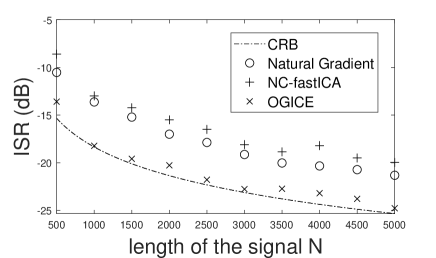
Figure 1: Average ISR for $d=5$, $\alpha=2$, and varying $N$.

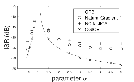
Figure 2: Average ISR for $d=5$, $N=2500$ and varying $\alpha$.

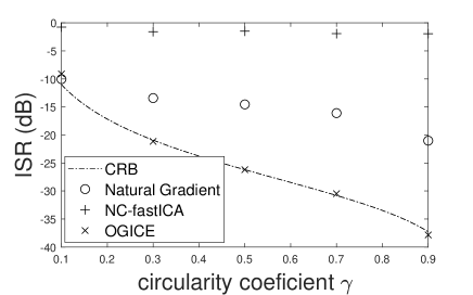
Figure 3: Average ISR for $d=5$, $N=2500$, $\alpha=1$ and varying circularity coefficient $\gamma$.

5.1.2 Non-Gaussian Background

As shown in Section 2.7, there is a coincidence between the CRIBs for ICA and ICE when, in ICE, the non-Gaussianity of background is taken into account. In this section, we simulate the case mentioned at the end of that section, that is, when background signals are dependent (a transformation decomposing them into independent components as assumed in ICA need not to exist). The theoretical CRIB for this simulation is given by (46).

In a trial, $d=4$ real-valued signals are generated. The background is drawn according to the joint pdf given by

$$p(z^{1},\dots,z^{d-1})\propto\exp\left(-\left({\lambda\sum_{i=1}^{d-1}|{z^{i}}|^{2}}\right)^{\alpha}\right)$$ (87)

where $\lambda>0$, and $\alpha\neq 1$ (for $\alpha=1$, the pdf is Gaussian). To scale the marginal pdfs of background signals to the unit variance, we put $\lambda=\frac{\Gamma\left(\frac{5}{2\alpha}\right)}{3\Gamma\left(\frac{3}{2\alpha}\right)}$. Then, it holds that

$$(\boldsymbol{\kappa}_{{\bf z}})_{kk}=\frac{4}{3}\lambda\alpha^{2}\frac{\Gamma(2+\frac{1}{2\alpha})}{\Gamma(\frac{3}{2\alpha})}.$$ (88)

The SOI is drawn from the GGD with zero mean, unit variance and a shape parameter $\tilde{\alpha}$, where $\tilde{\alpha}=\alpha+1$. Thus, for $\alpha=1$, all signals in the mixture are Gaussian.

We compare three algorithms with the CRIB given by (46): OGICE [47], EFICA [49], and NG-OGICE [44]. OGICE is designed for ICE with Gaussian background, where the CRIB is given by (49) (which we show as well for the sake of completeness). EFICA is an asymptotically efficient ICA algorithm provided that all original signals are drawn from GGD. NG-OGICE is an ICE method considering the non-Gaussianity of background, in which the true multivariate score function of background must be known.

In Fig. 4, the ISRs averaged over 100 trials achieved by OGICE, EFICA and NG-OGICE are compared. The bound (46) is denoted by CRIB_NG-ICE and the one for the Gaussian background (49) is denoted by CRIB_ICE. The results show that the mean ISRs by OGICE are close to the bound given by (49) (which is in a good agreement with the results of asymptotic performance analyses (9) [40]). The results by EFICA and NG-OGICE are closer to (46). NG-OGICE is even slightly more accurate than EFICA, which is caused by a more accurate modeling of the background’s pdf.

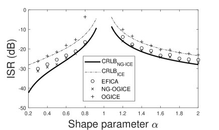
Figure 4: Average ISR for non-Gaussian background when pdfs of all signals are varying with respect to $\alpha$.

For $\alpha=1$, all signals are Gaussian, which means that the SOI cannot be separated from the background. With increasing non-Gaussianity of the mixture, which means increasing distance from $\alpha=1$, the separation accuracy gets better.

5.2 Piecewise Determined Mixtures with Circular Gaussian Background

To validate the bounds for CMV and CSV, both are compared with empirical results achieved by block-wise versions of OGICE introduced in [3]. The methods will be jointly referred to as BOGICE (in [3], BOGICE_a is the variant for CMV while BOGICE_w is for CSV). It should be noted that no other methods for CMV/CSV currently exist in the literature to our best knowledge.

In experiments here, we consider two statistical models of signals: The SOI is i.i.d. non-Gaussian over all blocks and i.i.d. SOI within blocks with the same distribution but varying variance over blocks. The background is assumed circular Gaussian i.i.d. with unit variance in all blocks in both cases.

In trials, $d=5$ independent complex-valued signals are generated. The SOI is drawn from a circular complex GGD with zero mean, unit variance, $\alpha=2$. The other signals are circular Gaussian, which corresponds to $\alpha=1$. The nonlinearity is given by the true score function. $M$ blocks of the same length are considered. Each block is mixed by a random mixing matrix. The mixing matrices obey the mixing models CMV or CSV, respectively.

The empirical ISRs achieved by BOGICE are compared with the CRIB corresponding to the mixing model used in the given simulation. To compare, we always show also the hypothetical CRIB achieved when the alternative mixing model was considered with the same statistical properties of the SOI.

5.2.1 An i.i.d. SOI

Fig. 5 corresponds to the simulation considering the CMV model for varying number of blocks, that is, $M=1,2,5,10$. It shows bar chart of ISR achieved by BOGICE averaged over 500 trials and the CRIB given by (71) (CMV) and, for comparison, also the CRIBs (70) (BICE) and (72) (CSV).

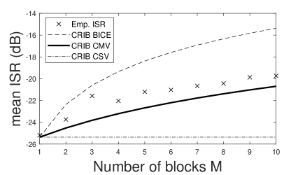
Figure 5: Average ISR for CMV mixing model when $d=5$, $N=5040$, and varying number of blocks $M$.

Similar simulation was done with the CSV model; the results are shown in Fig. 6 in the same fashion as in Fig. 5.

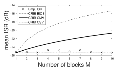
Figure 6: Average ISR for CSV mixing model when $d=5$, $N=5040$, and varying number of blocks $M$.

Figs. 5 and 6 show the coincidence between the empirical results by the variants of BOGICE and the CRIBs corresponding to the mixing model of the given simulation. The performances of the methods follow the same dependence on the number of blocks $M$ as these CRIBs. The results also show that BOGICE takes the advantage of the special mixing model CMV/CSV compared to BICE, as its mean ISR is lower that the CRIB (70), unless $M=1$ where all mixing models coincide.

The CRIBs by CSV are lower than those for CMV, which agrees with the results of Section 4. However, with this conclusion, the fact that both models are based on different assumptions must be also taken into account.

5.2.2 SOI with varying variance

In this special case, the SOI with the same pdf but varying variance over blocks is assumed. In a trial, $M=5$ blocks and four different settings of SOI’s variances are considered: Specifically, type A is $\sigma_{s^{m}}^{2}=1$ for $m=1,\dots,5$, type B corresponds to $\sigma_{s^{1}}^{2}=\sigma_{s^{2}}^{2}=1$, $\sigma_{s^{2}}^{2}=1$, $\sigma_{s^{4}}^{2}=\sigma_{s^{5}}^{2}=3$, type C shows $\sigma_{s^{m}}^{2}=m$, $m=1,\dots,5$ and type D is for $\sigma_{s^{m}}^{2}=m^{2}$, $m=1,\dots,5$.

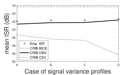
Figure 7: Average ISR for CMV mixing model when $d=5$, $N=5000$, and varying $\sigma_{s^{m}}$ over blocks.

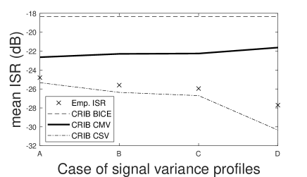
Figure 8: Average ISR for CMV mixing model when $d=5$, $N=5000$, and varying $\sigma_{s^{m}}$ over blocks.

In (74) and (75) is shown that the nonstationarity of the SOI improves the separation accuracy under the CSV mixing model, but worsen the accuracy under the CMV model.

The empirical results and so do the bounds show that for the increasing number of blocks $M$ the accuracy under the CMV mixing model drops, but under the CSV model it levels up. When the number of blocks is fixed and the variance of SOI differs on blocks then the results show that the higher the diversity of variance the better accuracy under CSV model, but lower under CMV model.

6 Conclusions

The derived CRLB on ISR achieved by complex ICE have shown that the structured (de-)mixing matrix model with a reduced number of parameters is not restrictive. The accuracy achievable by ICE with circular Gaussian background is asymptotically the same to that one of ICA when all but one signals are circular Gaussian. The CRLB shows that the general lower bound for ICA can be attained by the non-Gaussian ICE.

The piecewised determined model allows us to deal with dynamic mixtures thanks to its block structure. The CRLB of this model shows how the performance is limited by the number of blocks and that it can benefit from a varying variance of signals over blocks. Numerical simulations have confirmed the validity of the CRIBs.

References

- [1] P. Comon and C. Jutten, Handbook of Blind Source Separation: Independent Component Analysis and Applications, ser. Independent Component Analysis and Applications Series. Elsevier Science, 2010.
- [2] J. Eriksson and V. Koivunen, “Complex random vectors and ICA models: Identifiability, uniqueness, and separability,” in IEEE Trans. Information Theory, vol. 52, March 2006, pp. 1017–1029.
- [3] Z. Koldovský, J. Málek, and J. Janský, “Extraction of independent vector component from underdetermined mixtures through block-wise determined modeling,” in submitted, Oct. 2018.
- [4] Z. Koldovský and P. Tichavský, “Gradient algorithms for complex non-gaussian independent component/vector extraction, question of convergence,” IEEE Transactions on Signal Processing, vol. 67, no. 4, pp. 1050–1064, Feb 2019.
- [5] V. Kautský, Z. Koldovský, and P. Tichavský, “Cramér-Rao-induced bound for interference-to-signal ratio achievable through non-gaussian independent component extraction,” in 2017 IEEE International Workshop on Computational Advances in Multi-Sensor Adaptive Processing (CAMSAP), Dec 2017, pp. 94–97.
- [6] P. Smaragdis, “Blind separation of convolved mixtures in the frequency domain,” Neurocomputing, vol. 22, pp. 21–34, 1998.
- [7] T. Kim, H. T. Attias, S.-Y. Lee, and T.-W. Lee, “Blind source separation exploiting higher-order frequency dependencies,” IEEE Transactions on Audio, Speech, and Language Processing, pp. 70–79, Jan. 2007.
- [8] P. J. Huber, “Projection pursuit,” Ann. Statist., vol. 13, no. 2, pp. 435–475, June 1985.
- [9] J. Herault and C. Jutten, “Space or time adaptive signal processing by neural network models,” in AIP Conference Proceedings 151 on Neural Networks for Computing. Woodbury, NY, USA: American Institute of Physics Inc., 1987, pp. 206–211.
- [10] P. Comon, “Independent component analysis, a new concept?” Signal Processing, vol. 36, pp. 287–314, 1994.
- [11] J. F. Cardoso, “Blind signal separation: statistical principles,” Proceedings of the IEEE, vol. 86, no. 10, pp. 2009–2025, Oct 1998.
- [12] A. Hyvärinen, J. Karhunen, and E. Oja, Independent Component Analysis. John Wiley & Sons, 2001.
- [13] A. Cichocki and S. Amari, Adaptive Blind Signal and Image Processing. John Wiley & Sons, 2002.
- [14] T. Cover and J. Thomas, Elements of Information Theory. Wiley, 2006.
- [15] H. Sawada, R. Mukai, S. Araki, and S. Makino, “A robust and precise method for solving the permutation problem of frequency-domain blind source separation,” IEEE Transactions on Speech and Audio Processing, vol. 12, no. 5, pp. 530–538, Sep. 2004.
- [16] T. Adalı, Y. Levin-Schwartz, and V. D. Calhoun, “Multimodal data fusion using source separation: Two effective models based on ica and iva and their properties,” Proceedings of the IEEE, vol. 103, no. 9, pp. 1478–1493, Sep. 2015.
- [17] X. Chen, Z. J. Wang, and M. McKeown, “Joint blind source separation for neurophysiological data analysis: Multiset and multimodal methods,” IEEE Signal Processing Magazine, vol. 33, no. 3, pp. 86–107, May 2016.
- [18] I. Lee, T. Kim, and T.-W. Lee, “Fast fixed-point independent vector analysis algorithms for convolutive blind source separation,” Signal Processing, vol. 87, no. 8, pp. 1859–1871, 2007.
- [19] D. Kitamura, N. Ono, H. Sawada, H. Kameoka, and H. Saruwatari, “Determined blind source separation unifying independent vector analysis and nonnegative matrix factorization,” IEEE/ACM Transactions on Audio, Speech, and Language Processing, vol. 24, no. 9, pp. 1626–1641, 2016.
- [20] D. Kitamura, S. Mogami, Y. Mitsui, N. Takamune, H. Saruwatari, N. Ono, Y. Takahashi, and K. Kondo, “Generalized independent low-rank matrix analysis using heavy-tailed distributions for blind source separation,” EURASIP Journal on Advances in Signal Processing, vol. 2018, no. 1, p. 28, May 2018.
- [21] D.-T. Pham and J. F. Cardoso, “Blind separation of instantaneous mixtures of nonstationary sources,” IEEE Transactions on Signal Processing, vol. 49, no. 9, pp. 1837–1848, Sep 2001.
- [22] P. Tichavský and A. Yeredor, “Fast approximate joint diagonalization incorporating weight matrices,” IEEE Transactions on Signal Processing, vol. 57, no. 3, pp. 878–891, March 2009.
- [23] A. Yeredor, “Blind separation of gaussian sources with general covariance structures: Bounds and optimal estimation,” IEEE Transactions on Signal Processing, vol. 58, no. 10, pp. 5057–5068, Oct 2010.
- [24] Y. Li, T. Adalı, W. Wang, and V. D. Calhoun, “Joint blind source separation by multiset canonical correlation analysis,” IEEE Transactions on Signal Processing, vol. 57, no. 10, pp. 3918–3929, Oct 2009.
- [25] M. Anderson, T. Adali, and X. Li, “Joint blind source separation with multivariate gaussian model: Algorithms and performance analysis,” IEEE Transactions on Signal Processing, vol. 60, no. 4, pp. 1672–1683, April 2012.
- [26] D. Lahat and C. Jutten, “Joint independent subspace analysis using second-order statistics,” IEEE Transactions on Signal Processing, vol. 64, no. 18, pp. 4891–4904, Sept 2016.
- [27] L. D. Lathauwer and J. Castaing, “Blind identification of underdetermined mixtures by simultaneous matrix diagonalization,” IEEE Transactions on Signal Processing, vol. 56, no. 3, pp. 1096–1105, March 2008.
- [28] A. Ferreol, L. Albera, and P. Chevalier, “Fourth-order blind identification of underdetermined mixtures of sources (fobium),” IEEE Transactions on Signal Processing, vol. 53, no. 5, pp. 1640–1653, May 2005.
- [29] P. Comon and M. Rajih, “Blind identification of under-determined mixtures based on the characteristic function,” Signal Processing, vol. 86, no. 9, pp. 2271 – 2281, 2006, special Section: Signal Processing in UWB Communications.
- [30] P. Tichavský and Z. Koldovský, “Weight adjusted tensor method for blind separation of underdetermined mixtures of nonstationary sources,” IEEE Transactions on Signal Processing, vol. 59, no. 3, pp. 1037–1047, March 2011.
- [31] Z. Koldovský, P. Tichavský, A. H. Phan, and A. Cichocki, “A two-stage mmse beamformer for underdetermined signal separation,” IEEE Signal Processing Letters, vol. 20, no. 12, pp. 1227–1230, Dec 2013.
- [32] O. Yilmaz and S. Rickard, “Blind separation of speech mixtures via time-frequency masking,” IEEE Transactions on Signal Processing, vol. 52, no. 7, pp. 1830–1847, Jul. 2004.
- [33] S. Araki, S. Makino, A. Blin, R. Mukai, and H. Sawada, “Underdetermined blind separation of convolutive mixtures of speech by combining time-frequency masks and ICA,” in Proc. of the 18th International Congress on Acoustics (ICA 2004), vol. I, Apr. 2004, pp. 321–324.
- [34] F. Abrard and Y. Deville, “A time–frequency blind signal separation method applicable to underdetermined mixtures of dependent sources,” Signal Processing, vol. 85, no. 7, pp. 1389 – 1403, 2005.
- [35] Y. Li, S. Amari, A. Cichocki, D. W. C. Ho, and S. Xie, “Underdetermined blind source separation based on sparse representation,” IEEE Transactions on Signal Processing, vol. 54, no. 2, pp. 423–437, Feb 2006.
- [36] B. Liu, V. G. Reju, and A. W. H. Khong, “A linear source recovery method for underdetermined mixtures of uncorrelated ar-model signals without sparseness,” IEEE Transactions on Signal Processing, vol. 62, no. 19, pp. 4947–4958, Oct 2014.
- [37] P. Tichavský, Z. Koldovský, and E. Oja, “Performance analysis of the fastica algorithm and Cramér-Rao bounds for linear independent component analysis,” IEEE Transactions on Signal Processing, vol. 54, no. 4, pp. 1189–1203, April 2006.
- [38] B. Loesch and B. Yang, “Cramér–Rao bound for circular and noncircular complex independent component analysis,” in IEEE Trans. Signal Processing, vol. 61, Jan 2013, pp. 365–379.
- [39] A. Hyvärinen, “One-unit contrast functions for independent component analysis: a statistical analysis,” in Neural Networks for Signal Processing VII. Proceedings of the 1997 IEEE Signal Processing Society Workshop, Sep 1997, pp. 388–397.
- [40] D.-T. A. Pham, “Blind partial separation of instantaneous mixtures of sources,” in Proceedings of International Conference on Independent Component Analysis and Signal Separation. Springer Berlin Heidelberg, 2006, pp. 868–875.
- [41] M. Novey, T. Adali, and A. Roy, “A complex generalized gaussian distribution–characterization, generation, and estimation,” in IEEE Trans. Signal Processing, vol. 58, March 2010, pp. 1427–1433.
- [42] T. Menni, E. Chaumette, P. Larzabal, and J. P. Barbot, “New results on deterministic Cramér–Rao bounds for real and complex parameters,” in IEEE Trans. Signal Processing, vol. 60, March 2012, pp. 1032–1049.
- [43] J. F. Cardoso and B. H. Laheld, “Equivariant adaptive source separation,” IEEE Transactions on Signal Processing, vol. 44, no. 12, pp. 3017–3030, Dec 1996.
- [44] Z. Koldovský, P. Tichavský, and N. Ono, “Orthogonally-constrained extraction of independent non-gaussian component from non-gaussian background without ICA,” in Latent Variable Analysis and Signal Separation, Y. Deville, S. Gannot, R. Mason, M. D. Plumbley, and D. Ward, Eds. Cham: Springer International Publishing, 2018, pp. 161–170.
- [45] Z. Koldovský, J. Málek, P. Tichavský, Y. Deville, and S. Hosseini, “Blind separation of piecewise stationary non-gaussian sources,” Signal Processing, vol. 89, no. 12, pp. 2570 – 2584, 2009, special Section: Visual Information Analysis for Security.
- [46] M. Novey and T. Adali, “On extending the complex fastica algorithm to noncircular sources,” in IEEE Trans. Signal Processing, vol. 56, May 2008, pp. 2148–2154.
- [47] Z. Koldovský, P. Tichavský, and V. Kautský, “Orthogonally constrained independent component extraction: Blind MPDR beamforming,” in Proceedings of European Signal Processing Conference, Sep. 2017, pp. 1195–1199.
- [48] S. Amari, A. Cichocki, and H. H. Yang, “A new learning algorithm for blind signal separation,” in Proceedings of Neural Information Processing Systems, 1996, pp. 757–763.
- [49] Z. Koldovský, P. Tichavský, and E. Oja, “Efficient variant of algorithm FastICA for independent component analysis attaining the Cramér-Rao lower bound,” IEEE Transactions on Neural Networks, vol. 17, no. 5, pp. 1265–1277, Sept 2006.