Exact regularized point particle (ERPP) method for particle-laden wall-bounded flows in the two-way coupling regime

Abstract

The Exact Regularized Point Particle (ERPP) method is extended to treat the inter-phase momentum coupling between particles and fluid in the presence of walls by accounting for the vorticity generation due to the particles close to solid boundaries. The ERPP method overcomes the limitations of other methods by allowing the simulation of an extensive parameter space (Stokes number, mass loading, particle-to-fluid density ratio and Reynolds number) and of particle spatial distributions that are uneven (few particles per computational cell). The enhanced ERPP method is explained in detail and validated by considering the global impulse balance. In conditions when particles are located close to the wall, a common scenario in wall-bounded turbulent flows, the main contribution to the total impulse arises from the particle-induced vorticity at the solid boundary. The method is applied to direct numerical simulations of particle-laden turbulent pipe flow in the two-way coupling regime to address the turbulence modulation. The effects of the mass loading, the Stokes number and the particle-to-fluid density ratio are investigated. The drag is either unaltered or increased by the particles with respect to the uncoupled case. No drag reduction is found in the parameter space considered. The momentum stress budget, which includes an extra stress contribution by the particles, provides the rationale behind the drag behaviour. The extra stress produces a momentum flux towards the wall that strongly modifies the viscous stress, the culprit of drag at solid boundaries.

1 Introduction

Particle laden turbulent flows are ubiquitous and challenging due to the multi-scale physics involved, see der Hoef et al. (2008). Turbulence has an important role in the motion of particles. The transport, entrainment and redeposition, Soldati & Marchioli (2009), of solid particles, such as coal dust, is crucial in determining the overall efficiency of energy plants, Buhre et al. (2005). In automotive applications, the spray formation, Marmottant & Villermaux (2004), and the ensuing fuel jets, Jenny et al. (2012), impact the overall efficiency of combustion. Physical phenomena such as inter-particle collisions, Post & Abraham (2002); Wang et al. (2009), and turbulent modification, Balachandar & Eaton (2010), play an important role. In many applications, the multi-scale nature of the phenomena involved calls for modelling both the fluid turbulence and the particle motion, see Meyer (2012); Peirano et al. (2006) for modelling strategies in Reynolds Averaged Navier Stokes (RANS) equations and Marchioli (2017); Innocenti et al. (2016) in Large Eddy Simulation (LES).

In the context of particle laden turbulent flow many studies have been conducted in the one-way coupling regime, see Elghobashi (1994) for a discussion of the different regimes of coupling between fluid and particles, both from experimental point of view see e.g. Kostinski & Shaw (2001); Lau & Nathan (2016) and Eidelman et al. (2009), and from numerical point of view, see e.g. Toschi & Bodenschatz (2009); Bec et al. (2007); Sardina et al. (2012b); Picano et al. (2011); Marchioli & Soldati (2002); Goto & Vassilicos (2006) and Battista et al. (2011). On the other hand, the two-way coupling regime, where the fluid/particle momentum exchange is significant, is still being thoroughly investigated and some open questions need to be addressed. The first one is related to the numerical technique employed to model a reliable fluid/particle interaction. The second is related to the physics and deals with the particle dynamics, their spatial distribution and most importantly, with the turbulence modulation.

In the literature, different techniques are used to model the fluid/particle interaction. The approaches mostly depend on the typical size of the particle, e.g. the diameter $d_{p}$, that has to be compared with the characteristic length scales of the turbulent flow, see e.g. the recent review paper by Elghobashi (2019). The conceptually simplest approach is to resolve the particle boundary on the computational grid and to enforce the no-slip conditions on each particle boundary (particle-resolved simulation). This technique has recently become viable due to the ever-increasing computing resources. Among many, the immersed boundary technique, Uhlmann (2005); Breugem (2012), is employed to simulate suspensions under different conditions, for example in sedimentation problems, Fornari et al. (2016a, b), or dense suspensions, Costa et al. (2018). Given the tremendous computational cost, such simulations can currently only tackle problems in simplified geometries where the scale of the particle is roughly 10 times larger than the dissipative scale of the turbulent flow and the choice of density ratio is limited.

In many applications, the typical particle diameter is comparable to, or even smaller, than the dissipative scale and the density ratio is relatively large. In these conditions, it is unaffordable to carry out particle-resolved simulations. Being small, the particles are modelled as material points which behave as concentrated momentum sources/sinks for the fluid via the hydrodynamic drag that the (small) particle experiences along its trajectory.

In wall-bounded turbulent flows, the particles segregate towards the wall, (Caporaloni et al., 1975; Young & Leeming, 1997). The phenomena is known as turbophoresis and is relevant since the particles close to the wall affect the turbulence in the buffer region where the production of turbulent kinetic energy occurs together with the generation of the vortical structures, see Bijlard et al. (2010); Dritselis & Vlachos (2008, 2011) and Richter & Sullivan (2014) for the analysis of the topological modification of the structures in the buffer region.

An important issue in wall-bounded turbulent flows is whether the disperse phase feedback produces an overall increase or decrease of the friction and whether the turbulent fluctuations are augmented or reduced by the particles. Zhao et al. (2010, 2013) found reduction of the friction, i.e. the flow rate in presence of particles is augmented with respect to the flow rate in absence of particles for the same pressure gradient that drives the turbulent channel flow. Picciotto et al. (2006) and Li et al. (2016a, b) considered the turbulence modulation in a boundary layer, showing an increase in the skin friction coefficient at the wall. Li et al. (2001) report that the overall drag might increase or decrease depending on the mass loading of the suspension and the particle Stokes number. Lee & Lee (2015) found an overall increase of the turbulent fluctuations for relatively small particles, and a decrease of the turbulent fluctuations for large particles. In contrast, Pan & Banerjee (1997) found an overall increase in drag in a channel flow.

All the simulations mentioned above exploit the classical Particle In Cell (PIC) approach introduced by Crowe et al. (1977), except for Pan & Banerjee (1997) who employed an alternative inter-phase momentum coupling based on the solution of a truncated steady Stokes flow for the disturbance flow produced by the particles. Simulations using PIC have been performed also in the pipe flow, see e.g. the DNS by Rani et al. (2004) and Vreman (2007), and Large-Eddy Simulation (LES) by Yamamoto & Okawa (2010). Recently, the effect of the wall roughness has been discussed by Vreman (2015) and De Marchis & Milici (2016).

From the experimental point of view, the motion, deposition, entrainment, spatial distribution and velocity profiles of the particles in a turbulent boundary layer have been addressed in Kaftori et al. (1995a, b) and Kaftori et al. (1998). The fluid velocity profiles show larger gradients close to the wall (drag increasing) and the turbulent velocity fluctuations are increased in the near wall region. These modifications are associated with an increase in wall shear stress. Similar results are found in the experiments by Wu et al. (2006); Li et al. (2012) and Righetti & Romano (2004). No substantial modification of the mean velocity profile has been reported by Kulick et al. (1994) where only turbulent fluctuations are depleted across the channel. In the geometry of the pipe, Tsuji et al. (1984) show an increase in wall shear stress as well as Hadinoto et al. (2005). See also other experiments by Caraman et al. (2003); Borée & Caraman (2005) and Ljus et al. (2002).

In the numerical simulations discussed, the inter-phase momentum coupling is mainly achieved using the PIC approach. Even though the approach is rather simple, it suffers from several drawbacks. Firstly, the backreaction field, that can be constructed given the configuration of the suspension, is grid dependent (Gualtieri et al., 2013). Secondly, the solution depends on how many particles per computational cell are available, see Gualtieri et al. (2013); Boivin et al. (1998) and the general discussion by Balachandar & Eaton (2010). The unphysical constraint on the number of particles per cell poses several limitations on the range of the dimensionless parameters (Stokes number, mass loading, particle-to-fluid density ratio and Reynolds number) that can be explored in the simulations, see the conclusion of Gualtieri et al. (2015). A further issue concerns the model required to compute the hydrodynamic force on each particle. In the simple model of the Stokes drag, the fluid velocity at the particle position must be correctly interpreted as the background fluid velocity, i.e. as the fluid velocity in absence of the disturbance flow produced by the specific particle under consideration. Unfortunately, in two-way coupled simulations, the unperturbed flow is unavailable unless specific techniques are exploited to remove the particle self-disturbance, see e.g. Horwitz & Mani (2016, 2017); Capecelatro & Desjardins (2013) and Ireland & Desjardins (2017); Akiki et al. (2017) where several methods are proposed to circumvent this problem. These considerations pose challenging issues from the theoretical point of view and call for more accurate modelling of the particle/fluid interaction. The Exact Regularized Point Particle (ERPP) method has been proven to correctly evaluate the particle hydrodynamic force since the particle self-disturbance flow is known in a closed form. Moreover, the approach provides convergent turbulent statistics at the smallest scales of the flow, see Gualtieri et al. (2017); Battista et al. (2018) .

The aim of the present manuscript is to generalise the ERPP method, originally derived for free space flows, for the simulation of particle-laden wall-bounded turbulent flows and to provide a parametric study of turbulence modulation in conditions inaccessible to the classical PIC method. A treatment of the particle phase which is not sufficiently accurate would produce an incorrect force field on the fluid, mostly in a narrow layer close to the bounding walls thus altering the delicate balance of momentum in the wall layer and may lead to unphysical macroscopic effects. Once particles form clusters and segregate near the wall, the force they exert on the fluid will depend on the cluster geometry and, since clusters are generated by the small turbulent scales, a non-convergent algorithm will poorly reproduce the overall physics, i.e. the modification of wall friction due to the particles. The extended ERPP method overcomes these issues and provides a systematic approach to accurately predict the dynamics of wall-bounded particle-laden turbulent flows free of numerical artefacts. After the basic dynamics is captured, more sophisticated observables can be addressed and trusted given the convergence properties of the approach, in order to address higher order statistics in shear dominated flows, Jacob et al. (2008), or the scale-by-scale dynamics, Mollicone et al. (2018).

Technological applications generally involve turbulent flows in a complex geometry. In view of providing a sufficiently general approach, it is important to include the effects of wall curvature when studying the inter-phase momentum exchange between particles and fluid close to solid boundaries. For this reason, the simplest flow configuration that can be addressed is the turbulent flow inside a circular pipe, which we simulate using direct numerical simulation. Most of the turbulent fluctuations are generated in the near wall region, see e.g.  Marusic et al. (2010, 2013); Mathis et al. (2009); Hwang & Cossu (2010), requiring an accurate modelling of the inter-phase momentum exchange close to solid walls.

The ERPP method enables a free choice of the control parameters, that is the Stokes number, mass loading, particle-to-fluid density ratio and Reynolds number, allowing to explore a region of the parameter space which is not possible for other approaches, such as the PIC method and resolved particle method. For example, when the particle-to-fluid density ratio is order $20-200$, the number of particles turns out to be small for a given grid resolution imposed by the Reynolds number. These values roughly correspond to cases involving medicinal particulate commonly used for inhalable drug delivery systems, carbon dust transport, food industry powders resulting from the processing of cereals and sawdust resulting from wood manufacturing. Another advantage arises when the carrier phase is relatively dense, such as water, resulting in relatively low density ratios considering common materials. The ERPP method also allows the simulation of flows where the particle spatial distribution is uneven and few particles per cell are found in some regions of the flow. This may occur, for example, in water steam flows where the condensation of small droplets, imposed by external thermodynamical conditions, dictates the number of particles in a specific flow region.

The paper is organised as follows: section 2 provides the theoretical background of the methodology for wall-bounded flows. Section 3 addresses the validation of the extended ERPP approach and section 4 discusses the simulation setup and parameters for the simulations of the turbulent pipe flow, the skin friction coefficient and the mean momentum balance. Section 5 summarises the main findings.

2 Methodology

The flow takes place in the domain ${\cal D}\backslash\Omega$ where $\cal D$ contains fluid and particles. $\Omega(t)=\cup_{p}\Omega_{p}(t)$, where $\Omega_{p}(t)$, $p=1,\ldots N_{p}$, is the domain occupied by the $p$-th particle with diameter $d_{p}$. The fluid is described by the incompressible Navier-Stokes equations with the no-slip condition at the solid boundaries

$$\begin{array}[]{l}\left.\begin{array}[]{l}\displaystyle\nabla\cdot{\bf u}=0\\ \\ \displaystyle\frac{\partial{\bf u}}{\partial t}+{\bf u}\cdot\nabla{\bf u}=-\frac{1}{\rho_{f}}\nabla{\rm p}+\nu\nabla^{2}{\bf u}\end{array}\right\}\qquad{\bf x}\in{\cal D}\backslash\Omega\\ \\ \displaystyle{\bf u}\lvert_{\partial\Omega_{p}(t)}={\bf V}_{p}({\bf x})\lvert_{\partial\Omega_{p}}\qquad\qquad p=1,\ldots,N_{p}\\ \\ \displaystyle{\bf u}^{(\pi)}\lvert_{\partial{\cal D}}=0\\ \\ \displaystyle{\bf u}\cdot{\bf n}\lvert_{\partial{\cal D}}=u^{(n)}\lvert_{\partial{\cal D}}=0\\ \\ \displaystyle{\bf u}({\bf x},0)={\bf u}_{0}({\bf x})\qquad\qquad{\bf x}\in{\cal D}\backslash\Omega^{0}\ .\end{array}$$ (1)

In eq. (1), ${\bf u}_{0}({\bf x})$ is the initial velocity field, $\rho_{f}$ the fluid density, $\nu$ the kinematic viscosity and $\Omega^{0}=\Omega(0)$. At the boundaries $\partial\Omega_{p}$ and $\partial{\cal D}$, impermeability and no-slip conditions are assumed. Superscript $n$ and $\pi$ denote normal and tangent components of a given vector.

The particles affect the carrier fluid through the no-slip condition at the moving particle surface $\partial\Omega_{p}(t)$ where the fluid matches the local rigid body velocity of the particle ${\bf V}_{p}({\bf x})={\bf v}_{p}+\mbox{\boldmath$\omega$}_{p}\times\left({\bf x}-{\bf x}_{p}\right)$. The idea is to account for the effect of the moving particles on the fluid by defining a suitable correction field for which, in the limit of small particles, a closed form expression can be provided.

Given the current time $t$, for small intervals $t+\tau$, $0\leq\tau\leq Dt$, the carrier flow velocity is decomposed into two parts, ${\bf u}({\bf x},t+\tau)={\bf w}+{\bf v}$, that will be referred to as the background and perturbation velocity, respectively. The field ${\bf w}({\bf x},\tau)$, where dependence on the parameter $t$ is dropped for notational simplicity, is assumed to satisfy the equations

$$\begin{array}[]{l}\begin{array}[]{l}\displaystyle\nabla\cdot{\bf w}=0\\ \\ \displaystyle\frac{\partial{\bf w}}{\partial\tau}+{\bf F}=-\frac{1}{\rho_{f}}\nabla\pi+\nu\nabla^{2}{\bf w}\end{array}\\ \\ \displaystyle{\bf w}^{(\pi)}\lvert_{\partial{\cal D}}=-{\bf v}^{(\pi)}\lvert_{\partial{\cal D}}\\ \\ \displaystyle{\bf w}\cdot{\bf n}\lvert_{\partial{\cal D}}=w^{(n)}\lvert_{\partial{\cal D}}=0\\ \\ \displaystyle{\bf w}({\bf x},0)={\bf u}({\bf x},t)\,,\end{array}$$ (2)

where ${\bf x}\in{\cal D}$.

$${\bf F}=\left\{\begin{array}[]{ll}{\bf u}\cdot\nabla{\bf u}&\qquad\mbox{for}\,\,{\bf x}\in{\cal D}\backslash\Omega\\ \\ {\bf V}_{p}\cdot\nabla{\bf V}_{p}&\qquad\mbox{for}\,\,{\bf x}\in\Omega\end{array}\right.\,,$$ (3)

defined in $\cal D$, reproduces the convective term of the Navier-Stokes equation in the fluid domain ${\cal D}\backslash\Omega$ and is prolonged inside each particle using the corresponding rigid body particle velocity. For the present considerations, $\bf F$ can be treated as a prescribed forcing term. Note that, concerning $\bf w$, no boundary conditions are applied to the particle surfaces.

The field ${\bf v}({\bf x},\tau)$ exactly satisfies the linear unsteady Stokes equations (the full non-linear term being retained in the equation for ${\bf w}$),

$$\begin{array}[]{l}\left.\begin{array}[]{l}\displaystyle\nabla\cdot{\bf v}=0\\ \\ \displaystyle\frac{\partial{\bf v}}{\partial\tau}=-\frac{1}{\rho_{f}}\nabla{\rm q}+\nu\nabla^{2}{{\bf v}}\end{array}\right\}\qquad{\bf x}\in{\cal D}\backslash\Omega\\ \\ \displaystyle{\bf v}\lvert_{\partial\Omega_{p}}={\bf V}_{p}({\bf x})\ \lvert_{\partial\Omega_{p}}-{\bf w}\lvert_{\partial\Omega_{p}}\qquad p=1,\ldots N_{p}\\ \\ \displaystyle{\bf v}\cdot{\bf n}\lvert_{\partial{\cal D}}=v^{(n)}\lvert_{\partial{\cal D}}=0\\ \\ \displaystyle\frac{\partial{\bf v}^{(\mbox{\boldmath$\pi$})}}{\partial n}\bigg{|}_{\partial{\cal D}}=0\\ \\ \displaystyle{\bf v}({\bf x},0)=0\qquad{\bf x}\in{\cal D}\backslash\Omega(\tau)\,.\end{array}$$ (4)

The field $\bf v$ is coupled to $\bf w$ through the boundary conditions at the particle surfaces. Symmetrically, $\bf w$ is coupled to $\bf v$ via the external boundary $\partial D$, where impermeability and free slip conditions are enforced on $\bf v$. The resulting field $\bf u$ satisfies the required impermeability and no-slip conditions at all (particles and external domain) solid boundaries.

Since the linear field $\bf v$ obeys homogenous initial conditions at the initial time $\tau=0$, a simplified integral representation, see e.g. Piva & Morino (1987), is available for ${\bf v}$,

$$v_{i}({\bf x},\tau)=\int_{0}^{\tau}d\tilde{\tau}\int_{\partial\Omega}t_{j}(\mbox{\boldmath$\xi$},\tilde{\tau})\hat{G}_{ij}({\bf x},\mbox{\boldmath$\xi$},\tau,\tilde{\tau})-v_{j}(\mbox{\boldmath$\xi$},\tilde{\tau}){\cal\hat{T}}_{ijk}({\bf x},\mbox{\boldmath$\xi$},\tau,\tilde{\tau})n_{k}(\mbox{\boldmath$\xi$})\,dS_{\mbox{\boldmath$\xi$}},$$ (5)

where $\hat{G}_{ij}({\bf x},\mbox{\boldmath$\xi$},\tau,\tilde{\tau})$ is the Green function, a second order Cartesian tensor, appropriate for a free-slip, impermeable, external boundary $\partial D$. Physically, $\hat{G}_{ij}$ is the $i$-th velocity component induced at position ${\bf x}$ and time $\tau$ due to a delta function-like impulsive force localised at $\xi$ acting at time $\tilde{\tau}$ in direction $j$. The stress tensor associated to such velocity field is ${\cal\hat{T}}_{ijk}({\bf x},\mbox{\boldmath$\xi$},\tau,\tilde{\tau})$. In principle, for a generic domain $\cal D$, the specific Green function can be evaluated numerically. For the present application, the much simpler free-space solution can be used when the particle is far from $\partial D$. Close to $\partial D$, the actual geometry can be approximated by the local tangent plane and the Green function obtained by the method of images. This idea consists in describing the effect of the wall through a mirrored particle (image particle) that, by superimposing its disturbance flow to the flow produced by the physical particle (note that the problem is linear), enforces the correct boundary condition at the wall, see e.g. Happel & Brenner (2012) or Blake & Chwang (1974). Equation (5) expresses ${\bf v}({\bf x},\tau)$ in terms of a time convolution and a boundary integral involving the (physical) stress vector $t_{j}(\mbox{\boldmath$\xi$},\tilde{\tau})$ and the perturbation velocity $v_{j}(\mbox{\boldmath$\xi$},\tilde{\tau})$ at the particle boundaries. (No integration on $\partial{\cal D}$ is needed since the domain Green function, or its approximation, is used).

Substituting the first order truncation of the Taylor series of $\hat{G}_{ij}({\bf x},\mbox{\boldmath$\xi$},t,\tau)$ and ${\cal\hat{T}}_{ijk}({\bf x},\mbox{\boldmath$\xi$},t,\tau)$, centered at the particle geometric centre ${\bf x}_{p}$, in equation (5) provides the far field disturbance velocity, $r_{p}/d_{p}\gg 1$, where $r_{p}=|{\bf x}-{\bf x}_{p}|$,

$$v_{i}({\bf x},\tau)=-\sum_{p}\int_{0}^{\tau}D^{p}_{j}(\tilde{\tau})\hat{G}_{ij}({\bf x},{\bf x}_{p},\tau,\tilde{\tau})\,d\tilde{\tau}\ .$$ (6)

The disturbance field is expressed in terms of the hydrodynamic force ${\bf D}_{p}(\tau)$ on the particles, with Cartesian components $D^{p}_{j}$, and obeys the partial differential equation

$$\begin{array}[]{l}\displaystyle\nabla\cdot{\bf v}=0\\ \\ \displaystyle\frac{\partial{\bf v}}{\partial\tau}-\nu\nabla^{2}{\bf v}+\frac{1}{\rho_{f}}\nabla{\rm q}=-\frac{1}{\rho_{f}}\sum_{p}{\bf D}_{p}(\tau)\,\delta\left[{\bf x}-{\bf x}_{p}(\tau)\right]+\tilde{{\bf D}}_{p}(\tau)\,\delta\left[{\bf x}-\tilde{{\bf x}}_{p}(\tau)\right]\\ \\ {\bf v}({\bf x},0)=0\ .\end{array}$$ (7)

In eq. (7), the boundary conditions on $\partial{\cal D}$ are enforced by using the method of images including the additional forcing terms due to the mirrored particles which are indicated by the tildes. The image system is obtained by reflection with respect to the local tangent plane according to $\tilde{{\bf x}}^{\pi}_{p}={\bf x}^{\pi}_{p}$, $\tilde{x}^{n}_{p}=-x^{n}_{p}$, $\tilde{{\bf D}}^{\pi}_{p}={\bf D}^{\pi}_{p}$, $\tilde{D}^{n}_{p}=-D^{n}_{p}$. The reflection to the local tangent plane is acceptable when the particle diameter is much smaller than the local curvature of the wall as will be carefully checked in section §3

Following the procedure described in detail in Gualtieri et al. (2015), the velocity field obeying eq. (7) can be non-canonically decomposed in the form ${\bf v}={\bf v}_{\mbox{\boldmath$\zeta$}}+\nabla\phi$, where the pseudo-velocity ${\bf v}_{\mbox{\boldmath$\zeta$}}$ is the solution of

$$\begin{array}[]{l}\displaystyle\frac{\partial{\bf v}_{\mbox{\boldmath$\zeta$}}}{\partial\tau}-\nu\nabla^{2}{\bf v}_{\mbox{\boldmath$\zeta$}}=-\frac{1}{\rho_{f}}\sum_{p}{\bf D}_{p}(\tau)\,\delta\left[{\bf x}-{\bf x}_{p}(\tau)\right]+\tilde{{\bf D}}_{p}(\tau)\,\delta\left[{\bf x}-\tilde{{\bf x}}_{p}(\tau)\right]\\ \\ {\bf v}_{\mbox{\boldmath$\zeta$}}({\bf x},0)=0\ .\end{array}$$ (8)

By taking the curl of eqs. (7) and (8) one realises that $\nabla\times{\bf v}_{\mbox{\boldmath$\zeta$}}=\nabla\times{\bf v}$ with $\nabla\cdot{\bf v}_{\mbox{\boldmath$\zeta$}}\neq 0$. The complete field ${\bf v}$ is retrieved by projection on solenoidal fields which requires $\nabla^{2}\phi=-\nabla\cdot{\bf v}_{\mbox{\boldmath$\zeta$}}$. The advantage of this procedure is twofold: i) the pseudo-velocity ${\bf v}_{\mbox{\boldmath$\zeta$}}$ is localised around the sources; ii) the correction field $\nabla\phi$ can be evaluated a posteriori with the same projection algorithm used to enforce zero divergence of the background velocity ${\bf w}$, see Gualtieri et al. (2017) for application to two-way coupled particle laden homogeneous shear flows. The field ${\bf v}_{\mbox{\boldmath$\zeta$}}$ can be expressed in terms of the integral representation for the (vector) heat equation, see e.g. Stakgold (2000),

$${\bf v}_{\mbox{\boldmath$\zeta$}}({\bf x},\tau)=-\frac{1}{\rho_{f}}\int_{0}^{\tau^{+}}{\bf D}_{p}(\tilde{\tau})g\left[{\bf x}-{\bf x}_{p}(\tilde{\tau}),\tau-\tilde{\tau}\right]+\tilde{{\bf D}}_{p}(\tilde{\tau})g\left[{\bf x}-\tilde{{\bf x}}_{p}(\tilde{\tau}),\tau-\tilde{\tau}\right]\,d\tilde{\tau}$$ (9)

where the method of images has been used as before to enforce the boundary conditions on $\partial D$ and the free space Green’s function reads

$$g({\bf x}-\mbox{\boldmath$\xi$},\tau-\tilde{\tau})=\frac{1}{\left[4\pi\,\nu(\tau-\tilde{\tau})\right]^{3/2}}\exp\left[-\frac{\lVert{\bf x}-\mbox{\boldmath$\xi$}\rVert^{2}}{4\nu(\tau-\tilde{\tau})}\right]\ .$$ (10)

${\bf v}_{\mbox{\boldmath$\zeta$}}$ is a singular field that can be regularised by limiting the upper integration limit to $\tau-\varepsilon_{R}$, with $\varepsilon_{R}<<1$ a small regularisation parameter. The partial differential equation for the regularised field turns out to be,

$$\begin{array}[]{ll}\displaystyle\frac{\partial{\bf v}_{{\mbox{\boldmath$\zeta$}}_{R}}}{\partial\tau}-\nu\nabla^{2}{\bf v}_{{\mbox{\boldmath$\zeta$}}_{R}}=-\frac{1}{\rho_{f}}&\left\{{\bf D}_{p}(\tau-\epsilon_{R})g\left[{\bf x}-{\bf x}_{p}(\tau-\epsilon_{R}),\epsilon_{R}\right]+\right.\\ &+\left.\tilde{{\bf D}}_{p}(\tau-\epsilon_{R})g\left[{\bf x}-\tilde{{\bf x}}_{p}(\tau-\epsilon_{R}),\epsilon_{R}\right]\right\}\,,\end{array}$$ (11)

where again the boundary conditions are taken int account through the method of images. It is noteworthy that the forcing field is now expressed as a collection of Gaussians with small but finite variance ($\sigma(\tau)=\sqrt{2\nu(\tau-\varepsilon_{R})}\geq\sigma_{R}=\sqrt{2\nu\varepsilon_{R}}$) that can be discretised on a finite grid, provided the grid size is smaller than the minimum variance ($Dx<\sigma_{R}$). Note that the effect of the image particle decays in space faster than exponentially, hence its contribution may be neglected when the particle distance from the walls equals a few variances, say $3\sigma_{R}$ Another crucial aspect to take into account is the time delay in the position and drag of the particles, evaluated at the earlier time instant $\tau-\varepsilon_{R}$. The regularisation procedure amounts to removing the effect of the vorticity generated by the drag force exerted by the particle on the fluid in the last time instants $\tilde{\tau}\geq\tau-\varepsilon_{R}$, eq. (9). Such singular vorticity field cannot be resolved by a finite grid. It is not however neglected, since it is taken into account at later times, after it is spread out by diffusion. This aspect is of paramount importance to guarantee exact momentum conservation in the particle-fluid interaction and prevent the incurred error to accumulate in time, see Gualtieri et al. (2015).

The two fields, ${\bf w}$ and ${\bf v}_{R}={\bf v}_{\mbox{\boldmath$\zeta$}_{R}}+\nabla\phi_{R}$ ($\phi_{R}$ being the potential correction needed to make ${\bf v}_{R}$ solenoidal) can now be recombined in the complete, regularised velocity ${\bf u}_{R}={\bf w}+{\bf v}_{R}$, whose evolution equation is

$$\begin{array}[]{ll}\displaystyle\nabla\cdot{\bf u}_{R}=0\\ \\ \displaystyle\frac{\partial{\bf u}_{R}}{\partial\tau}+{\bf u}_{R}\cdot\nabla{\bf u}_{R}=-\frac{1}{\rho_{f}}\nabla p+\nu\nabla^{2}{\bf u}_{R}-\frac{1}{\rho_{f}}\sum_{p}^{N_{p}}&\left\{{\bf D}_{p}(\tau-\epsilon_{R})\,g\left[{\bf x}-{\bf x}_{p}(\tau-\epsilon_{R}),\epsilon_{R}\right]\right.+\\ &\left.\tilde{{\bf D}}_{p}(\tau-\epsilon_{R})\,g\left[{\bf x}-\tilde{{\bf x}}_{p}(\tau-\epsilon_{R}),\epsilon_{R}\right]\right\}\\ \\ \displaystyle{\bf u}^{(\mbox{\boldmath$\pi$})}_{R}\lvert_{\partial{\cal D}}=0&\\ \\ \displaystyle{\bf u}\cdot{\bf n}=u^{(n)}_{R}\lvert_{\partial{\cal D}}=0&\\ \\ \displaystyle{\bf u}_{R}({\bf x},0)={\bf u}({\bf x},t)\ .&\end{array}$$ (12)

Finally, the no-slip condition on $\partial{\cal D}$ in presence of the perturbation induced by particles is worth discussing. The background field ${\bf w}$ can be interpreted as the superposition of two other fields, ${\bf w}=\bar{{\bf w}}+{\bf w}^{\prime}$. $\bar{{\bf w}}$, satisfying the Navier-Stokes equations where the standard advection term is replaced by ${\bf F}$, as in (3), with impermeability and no-slip at $\partial{\cal D}$ and initial condition $\bar{{\bf w}}({\bf x},0)={\bf u}({\bf x},t)$. Since the full non linear term is accounted for by $\bar{{\bf w}}$, ${\bf w}^{\prime}$ satifies the unsteady Stokes equations

$$\begin{array}[]{l}\displaystyle\nabla\cdot{\bf w}^{\prime}=0\\ \\ \displaystyle\frac{\partial{\bf w}^{\prime}}{\partial\tau}=-\frac{1}{\rho_{f}}\nabla\pi^{\prime}+\nu\nabla^{2}{\bf w}^{\prime}\\ \\ \displaystyle{\bf w}^{\prime}_{(\mbox{\boldmath$\pi$})}\lvert_{\partial{\cal D}}=-{\bf v}^{(\mbox{\boldmath$\pi$})}_{R}\lvert_{\partial{\cal D}}\\ \\ \displaystyle{\bf w}^{\prime}\cdot{\bf n}\lvert_{\partial{\cal D}}=w^{\prime}_{(n)}\lvert_{\partial{\cal D}}=0\\ \\ \displaystyle{\bf w}^{\prime}({\bf x},0)=0\,,\end{array}$$ (13)

where the slippage imposed on $\partial{\cal D}$ balances the slip velocity due to the particle disturbance field. This is a generalisation of the well-known Stokes first problem for a flat plate which starts moving impulsively from rest. As in this classical problem, the slip velocity at the wall can be interpreted as a vortex sheet which is subsequently diffused in the flow domain, (Benfatto & Pulvirenti, 1984), mimicking the mechanism of vorticity generation at the wall, see Morton (1984) and Casciola et al. (1996).

3 Validation

The method is validated by considering the global impulse balance. In free space, the coupling algorithm was already shown to conserve total momentum in Gualtieri et al. (2015). The conservation properties of the extended algorithm in presence of a solid wall are now discussed. The simple but stringent tests carried out are instrumental to turbulent wall-bounded flows where the particles are known to accumulate in the near wall region, making momentum exchange between particles, fluid and the solid wall crucial.

A basic test case considers the fluid motion induced by a constant force, ${\bf F}$, applied at a fixed point, ${\bf x}_{p}$, to the fluid initially at rest in presence of solid boundaries. A cylindrical domain ${\cal D}$, of circular cross-section with radius $R$, is considered and the field is assumed to be periodic in the axial direction $z$. In cylindrical coordinates, ${\bf x}_{p}=(r_{p},\theta_{p},z_{p})$, the applied force and the velocity field read ${\bf F}=(F_{r},F_{\theta},F_{z})$ and ${\bf u}=(u_{r},u_{\theta},u_{z})$, respectively. The radial wall-normal distance is denoted by $y_{p}=R-r_{p}$. The constant force is applied in the $z$-direction, ${\bf F}=(0,0,F_{0})$, and the impulse grows linearly in time, ${\bf I}={\bf F}\,t$.

Time integration of the global axial force balance, ${\partial I_{u}}/{\partial t}=D_{f}+F_{0}$, where $I_{u}(t)=\int_{{\cal D}}\rho_{f}u_{z}\,dV$ and $D_{f}=\int_{\partial{\cal D}}\mu\,{\partial u_{z}}/{\partial r}\,dS$ are the fluid impulse and the viscous drag force, respectively, yields

$$I_{u}(t)+I_{f}(t)=F_{0}\,t\,$$ (14)

where $I_{f}(t)=-\int_{0}^{t}D_{f}(\tau)d\tau$ is the impulse due to friction drag. In dimensionless form, the different terms take the form $\nu I_{u}/(F_{0}R^{2})=I^{*}_{u}(\nu t/R^{2})$. In the ERPP method, the new parameter $\nu\varepsilon_{R}/R^{2}$ appears associated with the regularisation time scale $\varepsilon_{R}$, e.g. $\nu I_{u}/(F_{0}R^{2})=I^{*}_{u}(\nu t/R^{2},y_{p}/R,\nu\varepsilon_{R}/R^{2})$,

$$I_{u}^{*}\left(\frac{\nu t}{R^{2}},\frac{y_{p}}{R},\frac{\nu\varepsilon_{R}}{R^{2}}\right)+I_{f}^{*}\left(\frac{\nu t}{R^{2}},\frac{y_{p}}{R},\frac{\nu\varepsilon_{R}}{R^{2}}\right)=\frac{\nu t}{R^{2}}\,,$$ (15)

where the original form (14) is recovered in the limit $\nu\varepsilon_{R}/R^{2}$ approaching zero. Figure 1(a) corresponds to a test case with the force applied close to the wall ($y_{p}/R=0.1$) and $\nu\varepsilon_{R}/R^{2}=4\cdot 10^{-3}$, and shows that the impulse balance is satisfied within numerical accuracy on the (external) time scale $R^{2}/\nu$. At steady state, the fluid impulse becomes constant and the drag impulse increases linearly with time, becoming dominant at large time. The correct evaluation of the friction drag impulse appears now in all its relevance for wall-bounded flows. Indeed, the approach we propose is able to generate vorticity at the wall in a physically consistent way as proved by the correct evaluation of the viscous shear stress at the wall. The relative error between the exact value of the total impulse $I_{E}$ and its numerical evaluation $I_{u}+I_{f}$ is shown in the inset of panel a). The error does not accumulate in time.

A more subtle test concerns the impulse balance on the (inner) time scale of the regularisation parameter. Using $\varepsilon_{R}$ as time in the dimensional analysis yields

$$I_{u}^{**}\left(\frac{t}{\varepsilon_{R}},\frac{y_{p}}{\sqrt{2\nu\varepsilon_{R}}},\frac{R}{\sqrt{2\nu\varepsilon_{R}}}\right)+I_{f}^{**}\left(\frac{t}{\varepsilon_{R}},\frac{y_{p}}{\sqrt{2\nu\varepsilon_{R}}},\frac{R}{\sqrt{2\nu\varepsilon_{R}}}\right)=\frac{t}{\varepsilon_{R}}\,,$$ (16)

where, e.g., $I_{u}/(F_{0}\varepsilon_{R})=I_{u}^{**}$ and, as in § 2, $\sqrt{2\nu\varepsilon_{R}}=\sigma_{R}$. This alternative dimensionless form stresses the behaviour of the solution on the time scale of the regularisation, corresponding to the diffusive length scale $\sigma_{R}$, which is of the order of the mesh size to be adopted in the numerical solution. The purpose of checking the impulse balance in the above form is a more stringent check of the boundary conditions. In the theoretical description of the approach, the Green’s function of the domain was approximated using the method of images, mirroring the source with respect to the local tangent plane at the boundary.

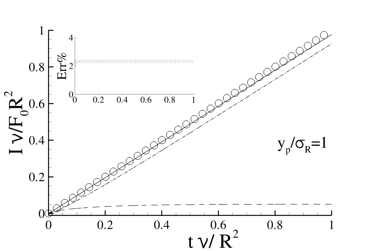
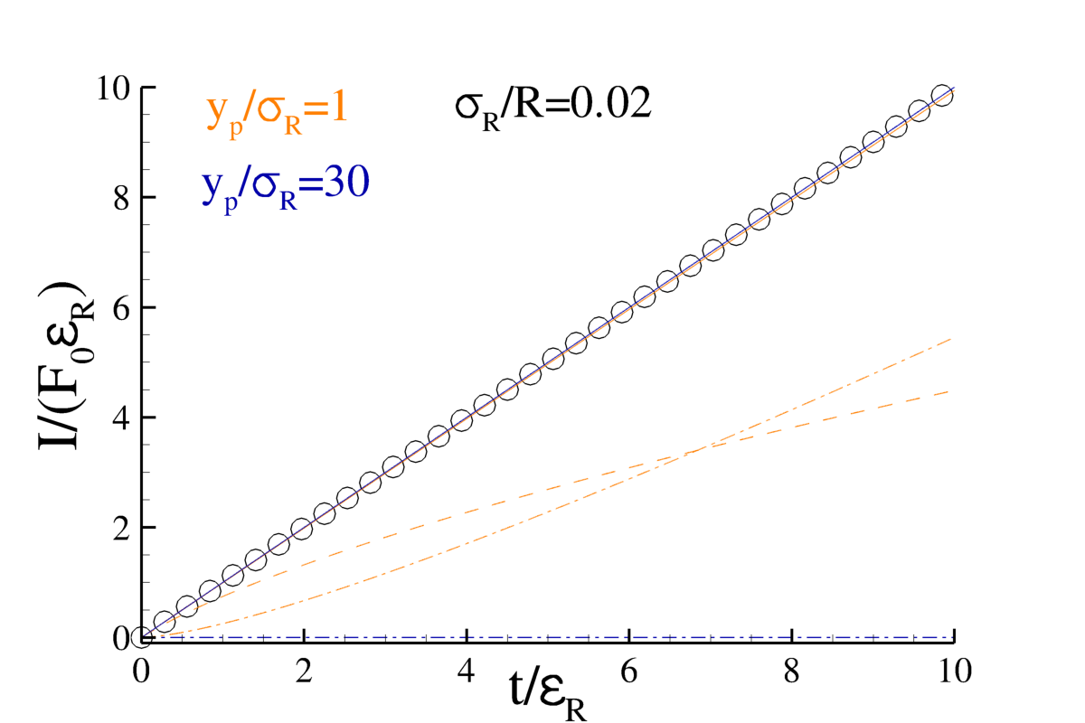
Figure 1: Impulse balance (14) for a constant force ${\bf F}=(0,0,F_{0})$ applied at a fixed point ${\bf x}_{p}$ at distance $y_{p}=R-r_{p}$ from the wall. The fluid is initially at rest in the cylindrical domain ${\cal D}$ with periodic boundary condition at $z=0$ and $z=2\pi$ and no-slip boundary conditions at $r=R$. Exact impulse $I_{E}=F_{0}\,t$ (open circles), $I_{u}(t)$ (dashed line), $I_{f}(t)$ (dash-doted line) and $I_{u}+I_{f}$ (solid line). Panel a): plot of the impulse normalised in external variables $\nu I/\left(F_{0}\,R^{2}\right)$ versus dimensionless time $\nu t/R^{2}$. The inset shows the normalised relative error $Err\%=100\,\cdot(I_{E}-I_{u}-I_{f})/I_{E}$. Panels b)-d): plot of the impulse normalised in internal variables $I/\left(F_{0}\,\epsilon_{R}\right)$ versus dimensionless time $t/\epsilon_{R}$. Panels b) and c): colours label different wall normal distances made dimensionless with the regularisation length-scale $\sigma_{R}$, namely $y_{p}/\sigma_{R}=1$ (orange lines) and $y_{p}/\sigma_{R}=30$ (blue lines) at $\sigma_{R}/R=0.02$. Panel b): cases with image point-force. Panel c): same cases as in panel b) without the image point-force. Panel d): the colours label the different regularisation length-scale $\sigma_{R}$ made dimensionless with the pipe radius $R$, namely $\sigma_{R}/R=0.02$ (orange lines) and $\sigma_{R}/R=0.2$ at for a point-force at fixed $y_{p}/\sigma_{R}=1$.

Figure 1(b) shows the impulse balance for two wall-normal distances of the point force. In one case $y_{p}/\sigma_{R}=1$ (orange solid line) the distance of the source from the wall is comparable to the regularisation length scale $\sigma_{R}$. In the other, $y_{p}/\sigma_{R}=30$ (blue solid line, almost totally superimposed on the orange one), the point force is relatively far from the wall. In both cases, the numerically evaluated impulse follows the exact solution (circles). In the first case (particle close to the wall) the fluid impulse, $I_{u}$ (orange dashed line) is initially comparable with the drag impulse $I_{f}$ (orange dash-dotted line). On the contrary, in the second case, when the force is applied far from the boundary, the friction drag is negligible on the observed (inner) time scale and the total impulse is almost all provided by the fluid. Overall, the result shows that the boundary condition and the associated vorticity generation is correctly captured by the algorithm. Panel c) illustrates the role of mirror image of the force by plotting results obtained by removing the image contribution. One expects that the effect of the image should be negligible when $y_{p}/\sigma_{R}\gg 1$. This is indeed the case, as shown by the comparison of the blue lines with the corresponding ones in panel b). On the contrary, when the distance of the application point is comparable with the regularisation length, $y_{p}/\sigma_{R}\leq 1$, the contribution of the image is crucial, as seen when comparing the orange solid lines with the corresponding ones in panel b). Since, for computational efficiency, the adopted Green’s function is only approximate, it is important to identify the range of validity of the approximation. The curvature of the wall, measured in terms of the regularisation length scale, is crucial parameter that determines the accuracy. Panel d) shows that, when $\sigma_{R}/R$ is sufficiently small (orange curves), the error is negligible. The error becomes larger as soon as this ratio increases (blue curves, wall curvature comparable with the regularisation length).

Figure 2 stresses the results of the previous figure, with emphasis on turbulent wall-bounded flows. As discussed in more detail in the following sections, inertial particles tend to accumulate in the viscous sublayer near the wall. The data reported in the figure artificially reproduce these conditions, by considering $N_{p}=100000$ randomly distributed point forces placed in an annular shell close to the cylindrical wall. As apparent in the plots, using the mirror images (orange curves) provides the total impulse. On the contrary, neglecting the images (blue symbols) completely spoils the quality of the simulation.

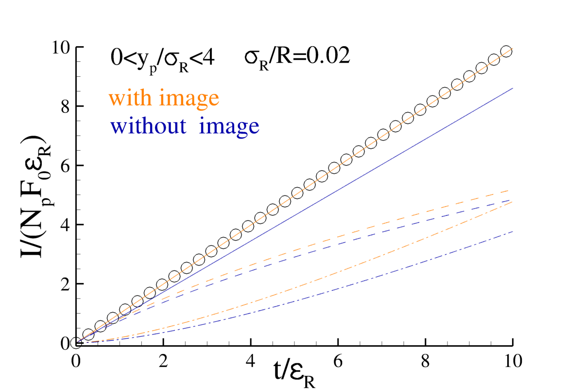
Figure 2: Impulse balance (14) for a constant force ${\bf F}=(0,0,F_{0})$ applied to $N_{p}$ fixed points ${\bf x}_{p}$ in the cylindrical domain ${\cal D}$ to the fluid initially at rest. The normalised impulse $I/\left(N_{p}\,F_{0}\,\epsilon_{R}\right)$ is plotted versus time $t$ made dimensionless with the regularisation time-scale $\epsilon_{R}$. Exact impulse $I_{E}$ (open circles), $I_{u}(t)$ (dashed line), $I_{f}(t)$ (dash-doted line) and $I_{u}+I_{f}$ (solid line). $N_{p}=100000$ point forces applied at points ${\bf x}_{p}$ randomly distributed in the stripe $0<y_{p}/\sigma_{R}<4$ near the wall for $\sigma_{R}/R=0.02$. The colours label cases with image point forces (orange lines) and without the images (blue line).

4 Particle-laden turbulent pipe flow

4.1 Simulation setup

The ERPP formulation is applied to a fully developed turbulent pipe flow. The dimensionless forms of equations (12) are solved in a cylindrical domain ${\cal D}=[0:R]\times[0:2\pi]\times[0:L_{z}]$ where the (dimensionless) pipe radius is $R=1$. Periodic boundary conditions are applied in the axial ($z$) direction, with $L_{z}=2\pi$. The subscript $R$ which is used to denote the regularised field will be dropped hereafter to ease notation. The reference quantities are the fluid density $\rho_{f}$, the pipe radius $R$, the bulk velocity of the purely Newtonian case $U_{b}=Q_{0}/(\pi R^{2})$, where $Q_{0}$ is the flow rate of the reference uncoupled case, and the viscosity $\mu$.

The flow is sustained by a constant mean pressure gradient applied in the direction of the axial unit vector ${\bf e}_{z}$, with the dimensionless pressure expressed as $P=dp/dz|_{0}(z-z_{0})+p(r,\theta,z,t)$,

$$\begin{array}[]{ll}\displaystyle\nabla\cdot{\bf u}=0\\ \\ \displaystyle\frac{\partial{\bf u}}{\partial t}+\nabla\cdot\left({\bf u}\otimes{\bf u}\right)=-\nabla p+\frac{1}{{\rm Re}_{b}}\nabla^{2}{\bf u}+{\bf f}-\frac{dp}{dz}\Big{|}_{0}{\bf e}_{z}\ .\end{array}$$ (17)

The Reynolds number is ${\rm Re}_{b}=U_{b}R/\nu$ and the field ${\bf f}$ is the particle feedback on the fluid

$${\bf f}=-\sum_{p}^{N_{p}}{\bf D}_{p}(t-\epsilon)\,g\left[{\bf x}-{\bf x}_{p}(t-\epsilon),\epsilon\right]+\tilde{{\bf D}}_{p}(t-\epsilon)\,g\left[{\bf x}-\tilde{{\bf x}}_{p}(t-\epsilon),\epsilon\right]\ .$$ (18)

The system consists of the carrier Newtonian fluid and of $N_{p}$ particles. The dimensionless drag force on the $p$-th particle is ${{\bf D}}_{p}=3\pi d_{p}/{\rm Re_{b}}\left({\bf u}|_{p}+d_{p}^{2}/24\nabla^{2}{\bf u}|_{p}-{\bf v}_{p}\right)$, where $d_{p}$ is the dimensionless particle diameter, ${\bf v}_{p}$ the particle velocity and ${\bf u}|_{p}={\bf u}({\bf x}_{p},t)$ is the fluid velocity at the particle position. Both the current time $t$ and the regularisation time scale $\epsilon_{R}$ are made dimensionless with $R/U_{b}$, that is $\epsilon=\epsilon_{R}U_{b}/R$.

$\phi$	$\rho_{p}/\rho_{f}$	$St_{+}$	$St_{0}$	$d_{p}^{+}$	$N_{p}$
0	-	-	-	-	-
0.1	180	10	0.82	1	122145
0.2	180	10	0.82	1	244290
0.4	180	10	0.82	1	488580
0.6	180	10	0.82	1	732870
0.4	180	15	1.23	1.23	265950
0.4	180	20	1.64	1.41	172739
0.4	180	80	6.54	2.82	21592
0.4	90	10	0.82	1.41	345479
0.4	360	10	0.82	0.70	690957
0.4	560	10	0.82	0.57	861775
0.4	900	10	0.82	0.45	1092499

Table 1: Simulation matrix. All runs are performed by imposing the same mean pressure gradient corresponding to a friction Reynolds number of $Re_{*}=180$. The bulk Reynolds number for the reference case where the particles do not back-react on the fluid (one-way coupling) is $Re_{b}=2650$. The grid resolution is $N_{\theta}\times N_{r}\times N_{z}=576\times 129\times 576$ corresponding to $\Delta r^{+}\big{|}_{w}=0.5$ at the wall and $\Delta r^{+}\big{|}_{0}=2$ at the centerline. The resolution in the azimuthal and axial directions is $(R\Delta\theta)_{+}=3.2$ and $\Delta z_{+}=3.2$, respectively. The mass loading is defined as $\phi=\rho_{p}N_{p}V_{p}/\rho_{f}V_{f}$ where $N_{p}$ is the number of particles, $V_{f}$ is the volume of the fluid in the domain ${\cal D}=[0:R]\times[0:2\pi]\times[0:L_{z}]$ and $\rho_{p}/\rho_{f}$ denotes the particle-to-fluid density ratio. $St_{+}$ is the Stokes number in internal units and $St_{0}$ is the Stokes number in external units, namely $St_{0}=\tau_{p}/\tau_{0}$ with $\tau_{0}=R/U_{b}$ being $U_{b}$, the bulk velocity in the uncoupled case. The column labeled $d_{p}^{+}$ shows the particle diameter in wall units. $N_{p}$ denotes the number of particles in the domain ${\cal D}$.

Impermeability and no-slip conditions are enforced at the pipe wall. Equations (17) are solved in cylindrical coordinates by exploiting a second order finite difference on a staggered grid, see Costantini et al. (2018); Battista et al. (2014). The classical Chorin’s projection method, Chorin (1968); Rannacher (1992), is used to enforce the divergence-free constraint imposed by the mass balance. Both convective and diffusive terms are explicitly integrated in time using a third-order low-storage Runge-Kutta method.

As customary, inner or wall units are given in terms of the viscous length $\ell_{*}=\nu/u_{*}$ and the friction velocity $u_{*}=\sqrt{\tau_{w}/\rho_{f}}$, with $\tau_{w}$ the average wall shear stress. The distance from the pipe wall in inner units is denoted $y_{+}=(1-r){\rm Re_{*}}$, where the friction Reynolds number is ${\rm Re}_{*}=u_{*}R/\nu$. The same distance in external units is denoted by $y=1-r$.

All the simulations are performed with the same friction Reynolds number $Re_{*}=180$. The corresponding bulk Reynolds number for a purely Newtonian (no particle backreaction) flow is $Re_{b}=2650$. The grid resolution is $N_{\theta}\times N_{r}\times N_{z}=576\times 129\times 576$ in the azimuthal, wall-normal and axial direction respectively. The grid in the radial direction is clustered near the wall with a minimum spacing of $\Delta r_{+}\big{|}_{w}=0.5$ which gradually increases towards the centreline reaching $\Delta r_{+}\big{|}_{0}=2$. The grid resolution in the azimuthal and axial direction is $(R\Delta\theta)_{+}=3.2$ and $\Delta z_{+}=3.2$ respectively.

Given the large particle-to-fluid density ratio $\rho_{p}/\rho_{f}$, the only relevant hydrodynamic force is the Stokes drag where the Faxen correction is accounted for, see Maxey & Riley (1983); Gatignol (1983). The Newton’s equations for the particles reduce to

$$\begin{array}[]{ll}\displaystyle\frac{d{\bf x}_{p}}{dt}={\bf v}_{p}\\ \\ \displaystyle\frac{d{\bf v}_{p}}{dt}=\frac{1}{{\rm St}_{b}}\left({\bf u}|_{p}+\frac{d_{p}^{2}}{24}\nabla^{2}{\bf u}|_{p}-{\bf v}_{p}\right)\,,\end{array}$$ (19)

where the bulk Stokes number is ${\rm St}_{b}=\tau_{p}U_{b}/R=\rho_{p}/(18\rho_{f}){\rm Re}_{b}d_{p}^{2}$, with $\tau_{p}$ the Stokes relaxation time of the particle.

In eqs. (19) and in the expression for the drag force (18), ${\bf u}|_{p}$ and $\nabla^{2}{\bf u}|_{p}$ are the fluid velocity and its Laplacian evaluated at the particle position taking into account the background fluid velocity including the disturbance of all the particles except the $p$-th one. This field is evaluated by summing the contributions of all the particles and by successively removing the particles’ self-disturbance. This step is easily performed with the ERPP approach where the self-disturbance velocity can be computed in a closed analytical form.

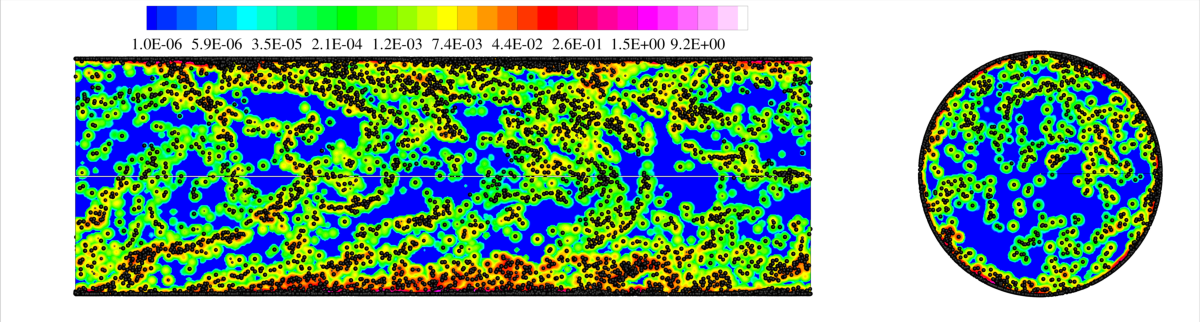
Figure 3: Snapshot of the particle back reaction field intensity (color) and particle configuration (black dots) for an instantaneous field at $\phi=0.4$, $St_{+}=10$ and $\rho_{p}/\rho_{f}=180$. The flow is from left to right.

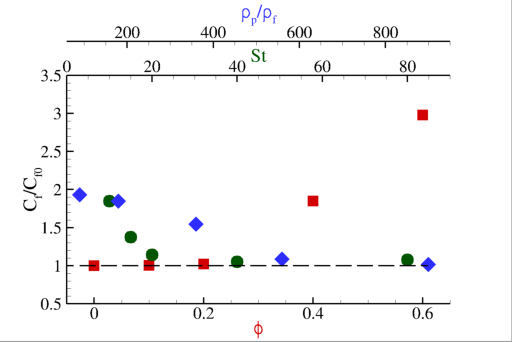
Figure 4: Friction coefficient of the two-way coupled simulations $C_{f}$ normalised with corresponding friction coefficient of the uncoupled case $C_{f0}$, see eq. (20). The dataset is plotted as a function of the the mass loading $\phi$ (red squares) at fixed $St_{+}=10$ and $\rho_{p}/\rho_{f}=180$, as a function of the Stokes number $St_{+}$ (green circles) at fixed $\phi=0.4$ and $\rho_{p}/\rho_{f}=180$, and as a function of the particle to fluid density ratio $\rho_{p}/\rho_{f}$ (blue diamonds) at fixed $\phi=0.4$ and $St_{+}=10$.

It is instrumental to introduce the inner Stokes number, ${\rm St}_{+}=\tau_{p}\ell_{*}/u_{*}={\rm St}_{0}{\rm Re}_{*}^{2}/{\rm Re}_{b}$. In two-way coupled simulations, a further dimensionless parameter that quantifies the particle backreaction on the fluid is the mass loading of the suspension. This is defined as the ratio between the total mass of the disperse phase and the fluid mass, $\phi=N_{p}\rho_{p}V_{p}/\rho_{f}V_{f}=(\rho_{p}/\rho_{f})N_{p}d_{p}^{2}/(12\pi)$, where $V_{p}$ is the volume of the particle and $V_{f}=\pi R^{3}L_{z}$ ($L_{z}=2\pi$ is the dimensionless axial extension of the domain) is the volume of the fluid in the domain ${\cal D}$. In the expression for the mass loading, $\phi_{V}=N_{p}V_{p}/V_{f}=N_{p}d_{p}^{2}/(12\pi)$ is the volume fraction.

In conclusion, the dynamics is controlled by a set of four dimensionless parameters, $\left\{Re_{*};\,St_{+};\,\phi;\,\rho_{p}/\rho_{f}\right\}$. The physical assumptions behind this description of the particle laden flow are: i) the density ratio $\rho_{p}/\rho_{f}$ is sufficiently large such that only the Stokes drag matters in the particle dynamics and ii) the particle diameter $d_{p}^{+}=d_{p}Re_{*}$ is small, which means that the particles are at most of the same order of magnitude of the viscous length.

The parameters for the different cases are summarised in table 1. The friction Reynolds number is fixed (i.e. the pressure drop is constant). The simulations are divided into three groups. In the first set, the mass loading $\phi$ is changed keeping Stokes number and density ratio fixed. The second set addresses the effects of the Stokes number at fixed mass loading and density ratio. Finally, the density ratio is changed at fixed mass loading and Stokes number to explore the effect of the number of particles.

A snapshot of the particle back-reaction intensity on the fluid and the instantaneous particle configuration is provided in figure 3 for the reference case at $\phi=0.4$, $St_{+}=10$ and $\rho_{p}/\rho_{f}=180$. Note the particle accumulation in the near-wall region and the strict correlation between the particle configuration and the Eulerian structure of the back reaction. Coherent particle structures extend from the wall up to the center of the pipe resembling the hairpin-like structures typical of wall-bounded flows.

4.2 Skin friction coefficient

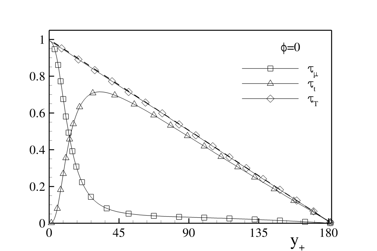
Figure 5: Normalized mean stress balance eq. (21) against wall-normal distance $y_{+}=(R-r)/y_{*}$. Viscous stress $\tau_{\mu}$ ($\square$), turbulent stress $\tau_{t}$ ($\triangle$), extra stress $\tau_{e}$ ($\bigcirc$), total stress $\tau_{T}=\tau_{\mu}+\tau_{t}+\tau_{e}$ ($\meddiamond$) and $\displaystyle\frac{dp}{dz}\Big{|}_{0}r$ (dashed line), (see text for definitions). All stresses are normalised with the wall shear stress $\tau_{w}$. Panel a): uncoupled case; Panel b): case $\phi=0.4$ and $St_{+}=10$; Panel c) case $\phi=0.6$ and $St_{+}=10$; d) same as panel c) but in semi-logarithmic scale.

Figure 6: Normalised mean stress balance eq. (5) against the wall-normal distance $y_{+}=(R-r)/y_{*}$. Viscous stress $\tau_{\mu}$ ($\square$), turbulent stress $\tau_{t}$ ($\triangle$), extra stress $\tau_{e}$ ($\bigcirc$), total stress $\tau_{T}=\tau_{\mu}+\tau_{t}+\tau_{e}$ ($\meddiamond$) and $\displaystyle\frac{dp}{dz}\Big{|}_{0}r$ (dashed line), (see text for definitions). All stresses are normalised with the wall shear stress $\tau_{w}$. Panel a) $\phi=0.4$, $St_{+}=10$; Panel b) $\phi=0.4$, $St_{+}=15$; Panel c) $\phi=0.4$, $St_{+}=20$; Panel d) $\phi=0.4$, $St_{+}=80$.

Figure 7: Normalised mean stress balance eq. (5) against the wall-normal distance $y_{+}=(R-r)/y_{*}$. Turbulent stress $\tau_{t}$ ($\square$), turbulent stress $\tau_{t}$ in the uncoupled case (solid line), extra stress $\tau_{e}$ ($\triangle$), $\tau_{t}+\tau_{e}$ ($\bigcirc$), and $\displaystyle\frac{dp}{dz}\Big{|}_{0}r$ (dashed line), see text for definitions. All stresses are normalised with the wall shear stress $\tau_{w}$. Panel a) $\phi=0.4$, $St_{+}=10$, $\rho_{p}/\rho_{f}=180$; Panel b) $\phi=0.4$, $St_{+}=80$, $\rho_{p}/\rho_{f}=180$;

The particles in fully developed turbulent pipe flow modify the drag with respect to the uncoupled (Newtonian) case. This alteration non-trivially depends on mass loading, Stokes number and particle-to-fluid density ratio. Figure 4 shows the friction coefficient

$$C_{f}=\frac{2\,\tau_{w}}{\rho_{f}U^{2}}=\frac{\left.dp/dz\right|_{0}}{\rho_{f}U^{2}}\,,$$ (20)

where $U=Q/(\pi R^{2})$ is the bulk velocity, $Q$ is the flow rate and $dp/dz|_{0}$ is the pressure gradient. In the figure $C_{f}$ is normalised with the unladen value, $C_{f0}$, and plotted as a function of mass loading (squares), Stokes number (circles) and particle-to-fluid density ratio (diamonds). Since the pressure drop is kept constant, an increase in friction coefficient corresponds to a decrease in mass flow rate. The figure shows that the drag increases at increasing mass loading and decreases with Stokes number and density ratio. In the present range of parameters, the friction coefficient is always grater or at most equal to the uncoupled case value.

Figure 8: Normalised mean stress balance eq. (5) against the wall-normal distance $y_{+}=(R-r)/y_{*}$. Viscous stress $\tau_{\mu}$ ($\square$), turbulent stress $\tau_{t}$ ($\triangle$), extra stress $\tau_{e}$ ($\bigcirc$), total stress $\tau_{T}=\tau_{\mu}+\tau_{t}+\tau_{e}$ ($\meddiamond$) and $\displaystyle\frac{dp}{dz}\Big{|}_{0}r$ (dashed line), (see text for definitions). All stresses are normalised with the wall shear stress $\tau_{w}$. In all panels $\phi=0.4$, $St_{+}=10$. Panel a) $\rho_{p}/\rho_{f}=90$; Panel b) $\rho_{p}/\rho_{f}=180$; Panel c) $\rho_{p}/\rho_{f}=360$; Panel d) $\rho_{p}/\rho_{f}=560$.

4.3 Mean momentum balance

The drag modification is attributed to the alteration of the different contributions to the stress balance, see e.g. Fukagata et al. (2002),

$$\mu\frac{\partial U_{z}}{\partial r}-\rho_{f}\langle u^{\prime}_{r}\,u^{\prime}_{z}\rangle+\frac{1}{r}\int_{0}^{r}\eta F_{z}\,d\eta=\frac{1}{2}{}\frac{dp}{dz}\Big{|}_{0}r\,,$$ (21)

where $U_{z}=\langle u_{z}\rangle$ is the mean axial velocity, $-\rho_{f}\langle u^{\prime}_{r}\,u^{\prime}_{z}\rangle$ is the turbulent Reynolds shear stress and $F_{z}=\langle f_{z}\rangle$ is the mean axial backreaction, with angular brackets denoting ensemble average and primed variables representing fluctuations.

Figure 9: Normalised mean viscous stress profiles against the wall-normal distance $y=(R-r)/R$. The inset report the mean velocity profile normalised with the bulk velocity, $V=U_{z}/U_{b}$, against the wall-normal distance close to the wall.

In absence of particles, the total shear stress, which is the sum of viscous stress, $\tau_{\mu}=\mu\partial U_{z}/\partial r$, and of turbulent Reynolds shear stress, $\tau_{t}=-\rho_{f}\langle u^{\prime}_{r}\,u^{\prime}_{z}\rangle$, is a linear function of the radial coordinate. This result can be derived by integrating once the mean axial momentum balance, see the classical textbook by Pope (2001). Following the same procedure, in presence of a disperse phase, the particle-induced extra stress, $\tau_{e}=\frac{1}{r}\int_{0}^{r}\eta F_{z}\,d\eta$, arises but the sum of the three stresses is still a linear function of the radial coordinate as imposed by the global axial momentum balance. This should not be taken for granted in a DNS, unless some care is devoted to reach the statistically steady state and acquire a well converged statistics. The critical cases correspond to large mass loading (large number of particles) and large Stokes number and/or small density ratio (small number of particles). The former due to the large computational cost, the latter due to the long runs required to have converged statistics.

Figure 5 shows the balance of eq. (21) for $\phi=0$ (uncoupled), $\phi=0.4$ and $\phi=0.6$ in panels a), b) and c), respectively. The turbulent stress is attenuated almost everywhere and its peak shifts towards the wall. Indeed, an extra stress arises that can be interpreted as an additional momentum flux towards the wall that modifies the turbulence dynamics and is at the origin of the drag increase. Its effect intensifies with increasing mass loading.

Figure 6 shows how the extra stress and the Reynolds shear stress profiles shift away from the wall at increasing Stokes number. As a consequence, the drag at $St_{+}=10$ is significantly higher than the drag at $St_{+}=80$ even though the extra stress has comparable values. Figure 7 goes deeper into the comparison with the uncoupled case, by considering $\tau_{t}+\tau_{e}$ at $St_{+}=10$ and $St_{+}=80$ and the turbulent Reynolds shear stress. At $St_{+}=10$, the profile of $\tau_{t}+\tau_{e}$ peaks much closer to the wall and is more intense than the uncoupled turbulent Reynolds stress profile. On the other hand, the distribution of $\tau_{t}+\tau_{e}$ closely reproduces the uncoupled Reynolds stress at $St_{+}=80$. This combination further explains the difference in the drag between $St_{+}=10$ and $St_{+}=80$.

To complete the discussion about the friction coefficients, the effect of the particle-to-fluid density ratio on the stress contributions is shown in figure 8. The drag modification occurs since i) the extra stress decreases with increasing density ratio, becoming negligible at $\rho_{p}/\rho_{f}=560$ (the behaviour is similar at $\rho_{p}/\rho_{f}=900$ and is not shown), and ii) the turbulent Reynolds stress peak increases and departs from the wall region.

The particles’ feedback produces two concurrent effects: the depletion of the turbulent Reynolds shear stress and the presence of the particle extra stress. The latter produces an increase of momentum flux towards the wall. The extra stress is then mainly balanced by the viscous stress since the turbulent Reynolds shear stress approaches zero. The modification of the viscous stress results in a modification of the drag as shown in figure 4. To better highlight this behaviour, figure 9 reports the normalised mean viscous stress profiles as a function of the wall distance, with insets showing a closeup view of the normalised mean axial velocity profile. When the particle extra-stress provides a significant momentum flux towards the wall, the fluid velocity increases with respect to the uncoupled case. As a consequence, the viscous stress increases and the friction follows the same fate. The main modification of the stress balance clearly occurs close to the wall. The extended ERPP method has been designed to capture the particle/fluid interaction close to a solid boundary accounting for the correct rate of vorticity generation which, in turns, results in a physically consistent representation of the viscous shear stress and thus of the overall drag. This is a distinct characteristic of the present approach which allows the prediction of the increase in drag.

4.4 Mean particle concentration

The particle mean distribution is presented in figure 10 as a function of the wall-normal distance. The particle concentration is defined as $\displaystyle C(r)=(n_{p}/\Delta V_{r})/(N_{p}/V_{f})$, where $n_{p}$ is the number of particles in a cylindrical shell of volume $\Delta V_{r}=2\pi\,r\,\Delta r\,L_{z}$ placed at distance $r$ from the axis, $N_{p}$ is the total number of particles in the fluid domain $V_{f}$. The normalisation of $C(r)$ is chosen such that $C=1$ when the particles are homogeneously distributed throughout the fluid domain. In the one-way coupling regime, inertial particles tend to segregate in the near wall region. The preferential accumulation, i.e. the turbophoresis, see Caporaloni et al. (1975); Reeks (1983) and the review by Balachandar & Eaton (2010), is controlled by the Stokes number, see Marchioli & Soldati (2002); Sardina et al. (2012a) for the channel and the boundary layer respectively. We have checked that the concentration profiles for the present simulations operated in the one-way coupling regime, match the data reported by Picano et al. (2009) in a spatially developing pipe flow, and by Sardina et al. (2011) for a statistically steady pipe flow, by comparing the results when the flow has reached fully developed conditions (data not shown, Picano private communication). The question is whether the backreaction and the resulting turbulent modification is able to alter the particle accumulation across the pipe.
Figure 10 addresses the effect of (a) mass loading, (b) Stokes number and (c) density ratio. At low mass loading ($\phi=0.2$) the particle concentration through the pipe decreases and particles segregate more at the wall. The opposite occurs when the mass loading increases. Concerning the Stokes number, the backreaction is effective in modifying the particle concentration with respect to the uncoupled case only for the populations at $St_{+}=10$ and $St_{+}=15$. Even at high Stokes number ($St_{+}=80$), the particles are still unevenly distributed across the flow domain. In the previous section, negligible turbulence modification was seen for this Stokes number, therefore, accumulation of particles is not necessarily the only precursor for turbulence modification. Panel c) addresses the effect of the density ratio. The solid line, representing the concentration in the one-way coupling regime, is the same for all cases since it only depends on the Stokes number. The trend of particle concentration in the bulk of the flow is not monotonic, the highest being at $\rho_{p}/\rho_{f}=180$. The opposite behaviour is observed at the wall. Unlike the uncoupled case, the density ratio is a further crucial parameter in the two-way regime that influences the particle concentration.

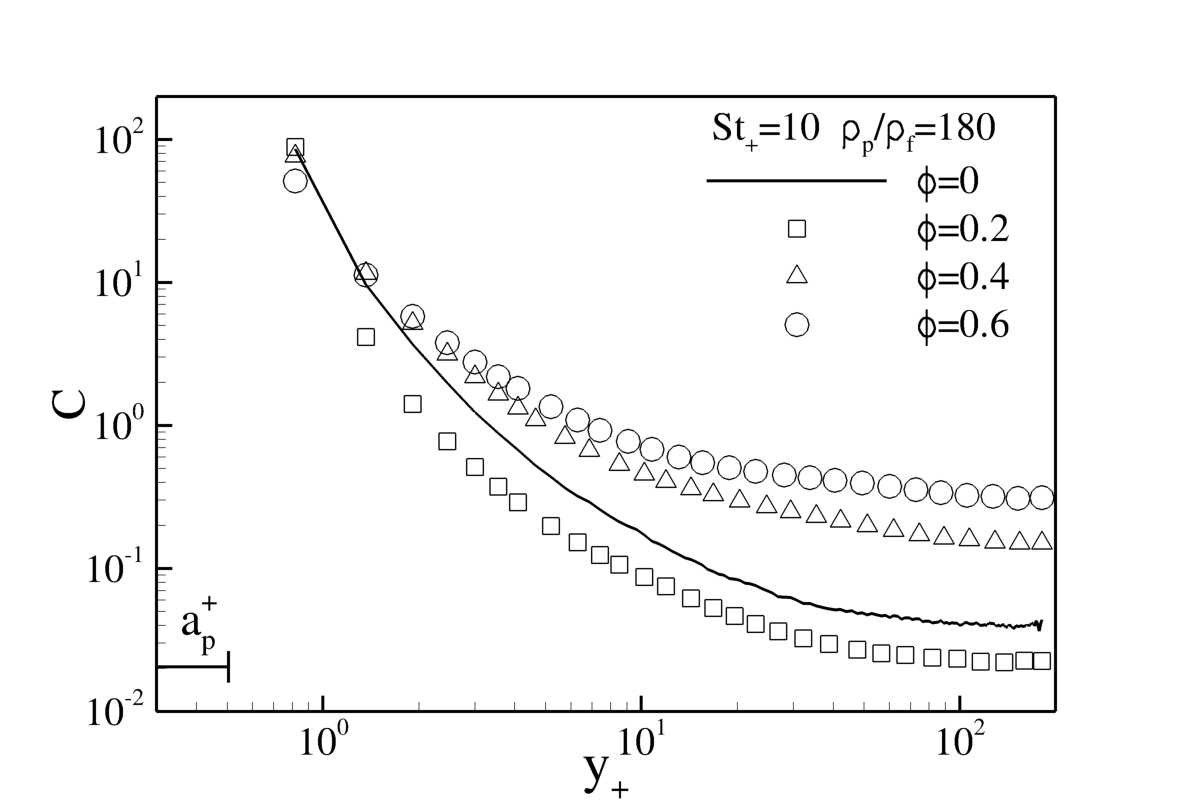
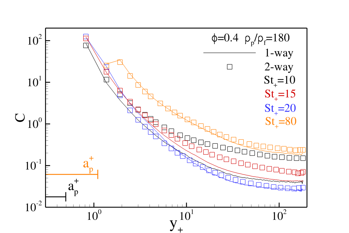
Figure 10: Mean particle concentration $C$ against the wall normal distance $y=(R-r)/y_{*}$. The lines refer the particle concentration in the uncoupled case whilst the symbols show the concentration in the two-way regime. The nominal particle radius is indicated with a horizontal line with the same color code of the data in the plots. Panel a): data at $St_{+}=10$ and $\rho_{p}/\rho_{f}=180$ and different mass load, $\phi=0.2$ ($\square$), $\phi=0.4$ ($\triangle$) and $\phi=0.6$ ($\bigcirc$). Panel b): effect of Stokes number, $St_{+}=10$ (black), $St_{+}=15$ (red), $St_{+}=20$ (blue) and $St_{+}=80$ (orange). Panel c): effect of the density ratio $\rho_{p}/\rho_{f}=90$ (black), $\rho_{p}/\rho_{f}=180$ (red), $\rho_{p}/\rho_{f}=360$ (blue), $\rho_{p}/\rho_{f}=560$ (orange).

5 Final remarks

A proper methodology to account for the inter-phase momentum exchange between inertial particles and the carrier flow in presence of wall has been developed. The approach extends the original ERPP method to account for the additional physics introduced by the wall. The disturbance generated by small particles can still be evaluated in a closed form by considering the associated unsteady Stokes problem in the half-space where only the impermeability boundary condition is enforced at the wall. When the disturbance is transferred to the background flow, the no-slip boundary condition is enforced by the Navier-Stokes solver of the carrier phase. From a physical point of view, this step corresponds to the generation and diffusion of the vorticity generated by the particles close to the wall. The approach has been carefully validated, showing how the impulse generated by the particles is correctly transferred to the fluid impulse in the bulk and to the viscous drag force at the wall. These results highlight the need to consider a set of images for those particles that lie close to the wall in order to reproduce the correct physics of the inter-phase momentum coupling.

The second part of the paper addresses the extended ERPP approach applied to direct numerical simulations of particle-laden fully developed turbulent pipe flow. The physical consistency of the inter-phase coupling method allows for a reliable analysis of the stress budget. In the near-wall region, the ERPP approach has been proven to capture the vorticity generated by the particles and the ensuing viscous shear stress. Results show a modification of the turbulent Reynolds shear stress and the important role played by the extra stress produced by the particles close to the wall. The physical interpretation corresponds to an augmented momentum flux towards the wall that ultimately increases the viscous shear stress and consequently the drag.

The approach applies to small particles, i.e. diameter comparable to the smallest hydrodynamical length-scale of the flow. The disturbance must be described by the unsteady Stokes equations, i.e. the particle Reynolds number is small. The suspension is considered diluted since inter-particles collisions and hydrodynamic interactions are neglected. No limitations are present on the density ratio, i.e. the approach can be used either for heavy particles or light bubbles. Clearly, in the latter case, added-mass and lift effects in the expression of the force on the bubble must be considered.

References

- Akiki et al. (2017) Akiki, G, Jackson, TL & Balachandar, S 2017 Pairwise interaction extended point-particle model for a random array of monodisperse spheres. Journal of Fluid Mechanics 813, 882–928.
- Balachandar & Eaton (2010) Balachandar, S. & Eaton, J.K. 2010 Turbulent dispersed multiphase flow. Ann. Rev. Fluid Mech 42, 111–133.
- Battista et al. (2018) Battista, F, Gualtieri, P, Mollicone, J-P & Casciola, CM 2018 Application of the exact regularized point particle method (erpp) to particle laden turbulent shear flows in the two-way coupling regime. International Journal of Multiphase Flow 101, 113–124.
- Battista et al. (2014) Battista, Francesco, Picano, Francesco & Casciola, Carlo Massimo 2014 Turbulent mixing of a slightly supercritical van der waals fluid at low-mach number. Physics of Fluids 26 (5), 055101.
- Battista et al. (2011) Battista, F, Picano, F, Troiani, G & Casciola, CM 2011 Intermittent features of inertial particle distributions in turbulent premixed flames. Physics of Fluids 23 (12), 123304.
- Bec et al. (2007) Bec, Jeremie, Biferale, Luca, Cencini, Massimo, Lanotte, Alessandra, Musacchio, Stefano & Toschi, Federico 2007 Heavy particle concentration in turbulence at dissipative and inertial scales. Physical review letters 98 (8), 084502.
- Benfatto & Pulvirenti (1984) Benfatto, G & Pulvirenti, M 1984 Generation of vorticity near the boundary in planar navier-stokes flows. Communications in mathematical physics 96 (1), 59–95.
- Bijlard et al. (2010) Bijlard, MJ, Oliemans, RVA, Portela, LM & Ooms, G 2010 Direct numerical simulation analysis of local flow topology in a particle-laden turbulent channel flow. Journal of Fluid Mechanics 653, 35–56.
- Blake & Chwang (1974) Blake, JR & Chwang, AT 1974 Fundamental singularities of viscous flow. Journal of Engineering Mathematics 8 (1), 23–29.
- Boivin et al. (1998) Boivin, Marc, Simonin, Olivier & Squires, Kyle D 1998 Direct numerical simulation of turbulence modulation by particles in isotropic turbulence. Journal of Fluid Mechanics 375, 235–263.
- Borée & Caraman (2005) Borée, J & Caraman, N 2005 Dilute bidispersed tube flow: Role of interclass collisions at increased loadings. Physics of Fluids 17 (5), 055108.
- Breugem (2012) Breugem, Wim-Paul 2012 A second-order accurate immersed boundary method for fully resolved simulations of particle-laden flows. Journal of Computational Physics 231 (13), 4469–4498.
- Buhre et al. (2005) Buhre, BJP, Elliott, LKr, Sheng, CD, Gupta, RP & Wall, TF 2005 Oxy-fuel combustion technology for coal-fired power generation. Progress in energy and combustion science 31 (4), 283–307.
- Capecelatro & Desjardins (2013) Capecelatro, Jesse & Desjardins, Olivier 2013 An euler–lagrange strategy for simulating particle-laden flows. Journal of Computational Physics 238, 1–31.
- Caporaloni et al. (1975) Caporaloni, M, Tampieri, F, Trombetti, F & Vittori, O 1975 Transfer of particles in nonisotropic air turbulence. Journal of the atmospheric sciences 32 (3), 565–568.
- Caraman et al. (2003) Caraman, N, Borée, J & Simonin, Olivier 2003 Effect of collisions on the dispersed phase fluctuation in a dilute tube flow: Experimental and theoretical analysis. Physics of Fluids 15 (12), 3602–3612.
- Casciola et al. (1996) Casciola, Carlo Massimo, Piva, R & Bassanini, P 1996 Vorticity generation on a flat surface in 3d flows. Journal of Computational Physics 129 (2), 345–356.
- Chorin (1968) Chorin, Alexandre Joel 1968 Numerical solution of the navier-stokes equations. Mathematics of computation 22 (104), 745–762.
- Costa et al. (2018) Costa, Pedro, Picano, Francesco, Brandt, Luca & Breugem, Wim-Paul 2018 Effects of the finite particle size in turbulent wall-bounded flows of dense suspensions. Journal of Fluid Mechanics 843, 450–478.
- Costantini et al. (2018) Costantini, Roberta, Mollicone, Jean-Paul & Battista, Francesco 2018 Drag reduction induced by superhydrophobic surfaces in turbulent pipe flow. Physics of Fluids 30 (2), 025102.
- Crowe et al. (1977) Crowe, C.T., Sharma, M.P. & Stock, D.E. 1977 The particle-source in cell method for gas droplet flow. J. Fluid Eng. 99, 325.
- De Marchis & Milici (2016) De Marchis, M & Milici, B 2016 Turbulence modulation by micro-particles in smooth and rough channels. Physics of Fluids 28 (11), 115101.
- Dritselis & Vlachos (2008) Dritselis, Chris D & Vlachos, Nicholas S 2008 Numerical study of educed coherent structures in the near-wall region of a particle-laden channel flow. Physics of Fluids 20 (5), 055103.
- Dritselis & Vlachos (2011) Dritselis, Chris D & Vlachos, Nicholas S 2011 Numerical investigation of momentum exchange between particles and coherent structures in low re turbulent channel flow. Physics of Fluids 23 (2), 025103.
- Eidelman et al. (2009) Eidelman, A, Elperin, T, Kleeorin, N, Hazak, G, Rogachevskii, I, Sadot, O & Sapir-Katiraie, I 2009 Mixing at the external boundary of a submerged turbulent jet. Physical Review E 79 (2), 026311.
- Elghobashi (1994) Elghobashi, S 1994 On predicting particle-laden turbulent flows. Applied Scientific Research 52 (4), 309–329.
- Elghobashi (2019) Elghobashi, Said 2019 Direct numerical simulation of turbulent flows laden with droplets or bubbles. Annual Review of Fluid Mechanics 51, 217–244.
- Fornari et al. (2016a) Fornari, Walter, Brandt, Luca, Chaudhuri, Pinaki, Lopez, Cyan Umbert, Mitra, Dhrubaditya & Picano, Francesco 2016a Rheology of confined non-brownian suspensions. Physical review letters 116 (1), 018301.
- Fornari et al. (2016b) Fornari, Walter, Picano, Francesco & Brandt, Luca 2016b Sedimentation of finite-size spheres in quiescent and turbulent environments. Journal of Fluid Mechanics 788, 640–669.
- Fukagata et al. (2002) Fukagata, Koji, Iwamoto, Kaoru & Kasagi, Nobuhide 2002 Contribution of reynolds stress distribution to the skin friction in wall-bounded flows. Physics of Fluids 14 (11), L73–L76.
- Gatignol (1983) Gatignol, R. 1983 The faxén formulas for a rigid particle in an unsteady non-uniform stokes-flow. Journal de Mécanique théorique et appliquée 2 (2), 143–160.
- Goto & Vassilicos (2006) Goto, Susumu & Vassilicos, JC 2006 Self-similar clustering of inertial particles and zero-acceleration points in fully developed two-dimensional turbulence. Physics of Fluids 18 (11), 115103.
- Gualtieri et al. (2017) Gualtieri, P, Battista, F & Casciola, CM 2017 Turbulence modulation in heavy-loaded suspensions of tiny particles. Physical Review Fluids 2 (3), 034304.
- Gualtieri et al. (2013) Gualtieri, P., Picano, F., Sardina, G. & Casciola, C.M. 2013 Clustering and turbulence modulation in particle-laden shear flow. J. Fluid Mech. 715, 134–162.
- Gualtieri et al. (2015) Gualtieri, Paolo, Picano, F, Sardina, Gaetano & Casciola, Carlo Massimo 2015 Exact regularized point particle method for multiphase flows in the two-way coupling regime. Journal of Fluid Mechanics 773, 520–561.
- Hadinoto et al. (2005) Hadinoto, K, Jones, EN, Yurteri, C & Curtis, JS 2005 Reynolds number dependence of gas-phase turbulence in gas–particle flows. International journal of multiphase flow 31 (4), 416–434.
- Happel & Brenner (2012) Happel, John & Brenner, Howard 2012 Low Reynolds number hydrodynamics: with special applications to particulate media, , vol. 1. Springer Science & Business Media.
- der Hoef et al. (2008) der Hoef, M.A. Van, Annald, M. Van Sint, Deen, N.G. & Kuipers, J.A.M. 2008 Numerical simulations of dense gas-solid fluidized beds: a multiscale modeling strategy. Ann. Rev. Fluid Mech 40, 47–70.
- Horwitz & Mani (2016) Horwitz, JAK & Mani, Ali 2016 Accurate calculation of stokes drag for point–particle tracking in two-way coupled flows. Journal of Computational Physics 318, 85–109.
- Horwitz & Mani (2017) Horwitz, Jeremy & Mani, Ali 2017 Correction scheme for point-particle two-way coupling applied to nonlinear drag law. arXiv preprint arXiv:1703.06966 .
- Hwang & Cossu (2010) Hwang, Yongyun & Cossu, Carlo 2010 Self-sustained process at large scales in turbulent channel flow. Physical review letters 105 (4), 044505.
- Innocenti et al. (2016) Innocenti, Alessio, Marchioli, Cristian & Chibbaro, Sergio 2016 Lagrangian filtered density function for les-based stochastic modelling of turbulent particle-laden flows. Physics of Fluids 28 (11), 115106.
- Ireland & Desjardins (2017) Ireland, Peter J & Desjardins, Olivier 2017 Improving particle drag predictions in euler–lagrange simulations with two-way coupling. Journal of Computational Physics 338, 405–430.
- Jacob et al. (2008) Jacob, Boris, Casciola, Carlo Massimo, Talamelli, Alessandro & Alfredsson, P Henrik 2008 Scaling of mixed structure functions in turbulent boundary layers. Physics of fluids 20 (4), 045101.
- Jenny et al. (2012) Jenny, Patrick, Roekaerts, Dirk & Beishuizen, Nijso 2012 Modeling of turbulent dilute spray combustion. Progress in Energy and Combustion Science .
- Kaftori et al. (1995a) Kaftori, D, Hetsroni, G & Banerjee, S 1995a Particle behavior in the turbulent boundary layer. i. motion, deposition, and entrainment. Physics of Fluids 7 (5), 1095–1106.
- Kaftori et al. (1995b) Kaftori, D, Hetsroni, G & Banerjee, S 1995b Particle behavior in the turbulent boundary layer. ii. velocity and distribution profiles. Physics of Fluids 7 (5), 1107–1121.
- Kaftori et al. (1998) Kaftori, D, Hetsroni, G & Banerjee, S 1998 The effect of particles on wall turbulence. International Journal of Multiphase Flow 24 (3), 359–386.
- Kostinski & Shaw (2001) Kostinski, Alexander B & Shaw, Raymond A 2001 Scale-dependent droplet clustering in turbulent clouds. Journal of fluid mechanics 434, 389–398.
- Kulick et al. (1994) Kulick, Jonathan D, Fessler, John R & Eaton, John K 1994 Particle response and turbulence modification in fully developed channel flow. Journal of Fluid Mechanics 277, 109–134.
- Lau & Nathan (2016) Lau, Timothy CW & Nathan, Graham J 2016 The effect of stokes number on particle velocity and concentration distributions in a well-characterised, turbulent, co-flowing two-phase jet. Journal of Fluid Mechanics 809, 72–110.
- Lee & Lee (2015) Lee, Junghoon & Lee, Changhoon 2015 Modification of particle-laden near-wall turbulence: Effect of stokes number. Physics of Fluids 27 (2), 023303.
- Li et al. (2016a) Li, Dong, Luo, Kun & Fan, Jianren 2016a Modulation of turbulence by dispersed solid particles in a spatially developing flat-plate boundary layer. Journal of Fluid Mechanics 802, 359–394.
- Li et al. (2016b) Li, Dong, Wei, Anyang, Luo, Kun & Fan, Jianren 2016b Direct numerical simulation of a particle-laden flow in a flat plate boundary layer. International Journal of Multiphase Flow 79, 124–143.
- Li et al. (2012) Li, Jing, Wang, Hanfeng, Liu, Zhaohui, Chen, Sheng & Zheng, Chuguang 2012 An experimental study on turbulence modification in the near-wall boundary layer of a dilute gas-particle channel flow. Experiments in fluids 53 (5), 1385–1403.
- Li et al. (2001) Li, Yiming, McLaughlin, John B, Kontomaris, K & Portela, L 2001 Numerical simulation of particle-laden turbulent channel flow. Physics of Fluids 13 (10), 2957–2967.
- Ljus et al. (2002) Ljus, Camilla, Johansson, Bert & Almstedt, Alf-Erik 2002 Turbulence modification by particles in a horizontal pipe flow. International journal of multiphase flow 28 (7), 1075–1090.
- Marchioli (2017) Marchioli, Cristian 2017 Large-eddy simulation of turbulent dispersed flows: a review of modelling approaches. Acta Mechanica 228 (3), 741–771.
- Marchioli & Soldati (2002) Marchioli, Cristian & Soldati, Alfredo 2002 Mechanisms for particle transfer and segregation in a turbulent boundary layer. Journal of fluid Mechanics 468, 283–315.
- Marmottant & Villermaux (2004) Marmottant, P & Villermaux, E 2004 On spray formation. Journal of fluid mechanics 498, 73–111.
- Marusic et al. (2010) Marusic, Ivan, McKeon, BJ, Monkewitz, PA, Nagib, HM, Smits, AJ & Sreenivasan, KR 2010 Wall-bounded turbulent flows at high reynolds numbers: recent advances and key issues. Physics of Fluids 22 (6), 065103.
- Marusic et al. (2013) Marusic, Ivan, Monty, Jason P, Hultmark, Marcus & Smits, Alexander J 2013 On the logarithmic region in wall turbulence. Journal of Fluid Mechanics 716.
- Mathis et al. (2009) Mathis, Romain, Hutchins, Nicholas & Marusic, Ivan 2009 Large-scale amplitude modulation of the small-scale structures in turbulent boundary layers. Journal of Fluid Mechanics 628, 311–337.
- Maxey & Riley (1983) Maxey, M.R. & Riley, J.J. 1983 Equation of motion for a small rigid sphere in a nonuniform flow. Phys. Fluids 26, 2437.
- Meyer (2012) Meyer, Daniel W 2012 Modelling of turbulence modulation in particle-or droplet-laden flows. Journal of Fluid Mechanics 706, 251–273.
- Mollicone et al. (2018) Mollicone, J-P, Battista, F, Gualtieri, P & Casciola, CM 2018 Turbulence dynamics in separated flows: The generalised kolmogorov equation for inhomogeneous anisotropic conditions. Journal of Fluid Mechanics 841, 1012–1039.
- Morton (1984) Morton, BR 1984 The generation and decay of vorticity. Geophysical & Astrophysical Fluid Dynamics 28 (3-4), 277–308.
- Pan & Banerjee (1997) Pan, Y & Banerjee, S 1997 Numerical investigation of the effects of large particles on wall-turbulence. Physics of Fluids 9 (12), 3786–3807.
- Peirano et al. (2006) Peirano, Eric, Chibbaro, Sergio, Pozorski, Jacek & Minier, J-P 2006 Mean-field/pdf numerical approach for polydispersed turbulent two-phase flows. Progress in energy and combustion science 32 (3), 315–371.
- Picano et al. (2011) Picano, F, Battista, F, Troiani, G & Casciola, Carlo Massimo 2011 Dynamics of piv seeding particles in turbulent premixed flames. Experiments in Fluids 50 (1), 75–88.
- Picano et al. (2009) Picano, F, Sardina, G & Casciola, CM 2009 Spatial development of particle-laden turbulent pipe flow. Physics of Fluids (1994-present) 21 (9), 093305.
- Picciotto et al. (2006) Picciotto, Maurizio, Giusti, Andrea, Marchioli, Cristian & Soldati, Alfredo 2006 Turbulence modulation by micro-particles in boundary layers. In IUTAM Symposium on Computational Approaches to Multiphase Flow, pp. 53–62. Springer.
- Piva & Morino (1987) Piva, Renzo & Morino, Luigi 1987 Vector green’s function method for unsteady navier-stokes equations. Meccanica 22 (2), 76–85.
- Pope (2001) Pope, Stephen B 2001 Turbulent flows.
- Post & Abraham (2002) Post, S.L. & Abraham, J. 2002 Modeling the outcome of drop-drop collisions in diesel sprays. Int. J. Mult. Flows 28 (6), 997–1019.
- Rani et al. (2004) Rani, Sarma L, Winkler, CM & Vanka, SP 2004 Numerical simulations of turbulence modulation by dense particles in a fully developed pipe flow. Powder Technology 141 (1), 80–99.
- Rannacher (1992) Rannacher, Rolf 1992 On chorin’s projection method for the incompressible navier-stokes equations. In The Navier-Stokes equations II—theory and numerical methods, pp. 167–183. Springer.
- Reeks (1983) Reeks, MW 1983 The transport of discrete particles in inhomogeneous turbulence. Journal of aerosol science 14 (6), 729–739.
- Richter & Sullivan (2014) Richter, David H & Sullivan, Peter P 2014 Modification of near-wall coherent structures by inertial particles. Physics of Fluids 26 (10), 103304.
- Righetti & Romano (2004) Righetti, M & Romano, Giovanni Paolo 2004 Particle–fluid interactions in a plane near-wall turbulent flow. Journal of Fluid Mechanics 505, 93–121.
- Sardina et al. (2011) Sardina, Gaetano, Picano, Francesco, Schlatter, Philipp, Brandt, Luca & Casciola, Carlo Massimo 2011 Large scale accumulation patterns of inertial particles in wall-bounded turbulent flow. Flow, turbulence and combustion 86 (3-4), 519–532.
- Sardina et al. (2012a) Sardina, G, Schlatter, Philipp, Brandt, Luca, Picano, F & Casciola, Carlo Massimo 2012a Wall accumulation and spatial localization in particle-laden wall flows. Journal of Fluid Mechanics 699, 50–78.
- Sardina et al. (2012b) Sardina, Gaetano, Schlatter, Philipp, Picano, Francesco, Casciola, CM, Brandt, Luca & Henningson, Dan Stafan 2012b Self-similar transport of inertial particles in a turbulent boundary layer. Journal of Fluid Mechanics 706, 584–596.
- Soldati & Marchioli (2009) Soldati, A. & Marchioli, C. 2009 Physics and modelling of turbulent particle deposition and entrainment: review of a systematic study. Int. J. Multiphase flow 35(9), 827–839.
- Stakgold (2000) Stakgold, Ivar 2000 Boundary Value Problems of Mathematical Physics: Volume 2. SIAM.
- Toschi & Bodenschatz (2009) Toschi, Federico & Bodenschatz, Eberhard 2009 Lagrangian properties of particles in turbulence. Annual review of fluid mechanics 41, 375–404.
- Tsuji et al. (1984) Tsuji, Yutaka, Morikawa, Yoshinobu & Shiomi, Hiroshi 1984 Ldv measurements of an air-solid two-phase flow in a vertical pipe. Journal of Fluid Mechanics 139, 417–434.
- Uhlmann (2005) Uhlmann, Markus 2005 An immersed boundary method with direct forcing for the simulation of particulate flows. Journal of Computational Physics 209 (2), 448–476.
- Vreman (2007) Vreman, AW 2007 Turbulence characteristics of particle-laden pipe flow. Journal of fluid mechanics 584, 235–279.
- Vreman (2015) Vreman, AW 2015 Turbulence attenuation in particle-laden flow in smooth and rough channels. Journal of Fluid Mechanics 773, 103.
- Wang et al. (2009) Wang, L. P., Rosa, B., Gao, H., He, G. & Jin, G. 2009 Turbulent collision of inertial particles: Point-particle based, hybrid simulations and beyond. Int. J. Mult. Flow 35 (9), 854–867.
- Wu et al. (2006) Wu, Yi, Wang, Hangfeng, Liu, Zhaohui, Li, Jing, Zhang, Liqi & Zheng, Chuguang 2006 Experimental investigation on turbulence modification in a horizontal channel flow at relatively low mass loading. Acta Mechanica Sinica 22 (2), 99–108.
- Yamamoto & Okawa (2010) Yamamoto, Yasushi & Okawa, Tomio 2010 Numerical study of particle concentration effect on deposition characteristics in turbulent pipe flows. Journal of nuclear science and technology 47 (10), 945–952.
- Young & Leeming (1997) Young, John & Leeming, Angus 1997 A theory of particle deposition in turbulent pipe flow. Journal of Fluid Mechanics 340, 129–159.
- Zhao et al. (2010) Zhao, LH, Andersson, Helge Ingolf & Gillissen, JJ 2010 Turbulence modulation and drag reduction by spherical particles. Physics of Fluids (1994-present) 22 (8), 081702.
- Zhao et al. (2013) Zhao, Lihao, Andersson, Helge I & Gillissen, Jurriaan JJ 2013 Interphasial energy transfer and particle dissipation in particle-laden wall turbulence. Journal of Fluid Mechanics 715, 32.