Threshold Policies for Online Knapsack

The Competitive Ratio of Threshold Policies for Online Unit-density Knapsack Problems

Will Ma Graduate School of Business, Columbia University, New York, NY 10027, wm2428@gsb.columbia.edu David Simchi-Levi Institute for Data, Systems, and Society, Department of Civil and Environmental Engineering, and Operations Research Center, Massachusetts Institute of Technology, Cambridge, MA 02139, dslevi@mit.edu Jinglong Zhao Institute for Data, Systems, and Society, Massachusetts Institute of Technology, Cambridge, MA 02139, jinglong@mit.edu

We study an online knapsack problem where the items arrive sequentially and must be either immediately packed into the knapsack or irrevocably discarded. Each item has a different size and the objective is to maximize the total size of items packed. We focus on the class of randomized algorithms which initially draw a threshold from some distribution, and then pack every fitting item whose size is at least that threshold. Threshold policies satisfy many desiderata including simplicity, fairness, and incentive-alignment. We derive two optimal threshold distributions, the first of which implies a competitive ratio of 0.432 relative to the optimal offline packing, and the second of which implies a competitive ratio of 0.428 relative to the optimal fractional packing.

We also consider the generalization to multiple knapsacks, where an arriving item has a different size in each knapsack and must be placed in at most one. This is equivalent to the AdWords problem where item truncation is not allowed. We derive a randomized threshold algorithm for this problem which is 0.214-competitive. We also show that any randomized algorithm for this problem cannot be more than 0.461-competitive, providing the first upper bound which is strictly less than 0.5.

This online knapsack problem finds applications in many areas, like supply chain ordering, online advertising, and healthcare scheduling, refugee integration, and crowdsourcing. We show how our optimal threshold distributions can be naturally implemented in the warehouses for a Latin American chain department store. We run simulations on their large-scale order data, which demonstrate the robustness of our proposed algorithms.

1 Introduction

Consider the following problem. There is a knapsack of size 1 and an unknown sequence of items with sizes at most 1. The items arrive one-by-one, and each item must be irrevocably either packed into the knapsack or discarded upon arrival. An item can be packed only if its size does not exceed the remaining knapsack capacity. The goal is to maximize the sum of sizes of packed items, i.e. maximize the total capacity filled.

The decision of whether to accept each item into the knapsack is made by an online algorithm, which does not know the sizes of future items, nor the number of future items. Meanwhile, for any sequence of items, one could consider its optimal offline packing knowing the entire sequence in advance. For $c\leq 1$, a fixed (but possibly randomized) online algorithm is said to be $c$-competitive if on any sequence, its (expected) capacity packed is at least $c$ times the optimal offline packing. We are interested in the highest-possible value of $c$, which is called the competitive ratio.

For this problem, randomization is necessary to achieve any non-trivial competitive ratio. Indeed, a deterministic algorithm, when faced with an initial item of a small size $\varepsilon>0$, must either accept or reject. If it accepts, then it achieves a poor ratio when the item is followed by an item of size 1, packing size $\varepsilon$ when the optimal packing has size 1. On the other hand, if it rejects, then it achieves a poor ratio when the sequence ends after the first item, packing 0 when the optimum is $\varepsilon$.

With randomization, a simple idea, originally due to Han et al. (2015), yields a $\frac{1}{2}$-competitive algorithm. First, a fair coin is flipped. If Heads, then the algorithm greedily packs any item that fits. If Tails, then the algorithm rejects all items until the first one that the greedy policy would not have fit, and starts to greedily accept items from that item (including that item). In expectation, this algorithm is $\frac{1}{2}$-competitive, since either the greedy packing (which the algorithm mimics half the time) is optimal, or the algorithm’s sum of capacity packed under the two outcomes exceeds 1, and hence its expected packing exceeds $\frac{1}{2}$, while the optimum is at most 1. Furthermore, it follows from the example above that $\frac{1}{2}$ is the competitive ratio for the class of all randomized algorithms.

1.1 Motivation for this Paper: Threshold Policies

In this paper, we derive the competitive ratio for a subclass of algorithms: (random) threshold algorithms. Threshold algorithms initially draw a threshold $\tau\in[0,1]$, and then accept every item of size at least $\tau$ that fits, but never change the threshold throughout the entire horizon after its initial draw. When $\tau=0$, the algorithm mimics the greedy algorithm.

Threshold algorithms constitute a natural subclass of algorithms with many benefits, as we outline below.

• Simplicity: First, threshold algorithms are logistically easy to implement, making non-adaptive accept/reject decisions that do not require recording the history of past items. We can use them to derive a random-threshold algorithm for a generalization of our problem to multiple knapsacks, as we discuss in Section 1.3.

• Applicability: Second, a threshold algorithm is characterized by a CDF $F$ for the threshold $\tau$, which has a simple interpretation for how to implement this randomized algorithm in practice. We implement simulations on an industry partner’s data, as we discuss in Section 1.4.

• Incentive-compatibility: Most importantly, threshold algorithms treat identical items equally, in a first-come-first-serve order, which implies that the items truthfully represent the demands for the knapsack.

  We elaborate on this incentive issue. In many applications, an arriving “item” corresponds to an order placed by a customer. Under a threshold algorithm, a customer is incentivized to place a single order for her desired amount, immediately upon her arrival. Indeed, there is no benefit to waiting since orders exceeding $\tau$ are first-come-first-served; moreover, should the customer’s order get rejected, there is no benefit to trying again later. Therefore, the sequence of items observed truthfully represents the desires of the customers, in order.

  By contrast, in the randomized algorithm described above (Han et al. 2015), a customer can easily manipulate the system. For example, if the first customer sees her order get rejected (because the coin in the algorithm landed Tails), then she can repeatedly try placing the same order again. After generating sufficiently many “fake” orders, the greedy policy cannot fit all the orders, and hence the algorithm will accept her order.

• Fairness: As a final note, our random-threshold algorithms “treat similar individuals similarly”, which is the definition of fairness proposed in Dwork et al. (2012). In particular, the probability of our random-threshold accepting an item (which fits) is dependent on only the size of that item, and moreover, this probability changes smoothly with respect to a change in size. Another notion of fairness in sequential decision-making was introduced by Gupta and Kamble (2019). Our random-threshold algorithms also satisfy their definition.

1.2 Techniques for Analyzing Threshold Policies

The analysis for the subclass of random threshold algorithms also becomes move involved, since a small change in $\tau$ could have a ripple effect on the items that fit and hence the items that are packed by the policy. We derive the best-possible CDF’s for threshold $\tau$, and hence the tight competitive ratio for threshold algorithms, under two different definitions of the optimal offline packing:

1. A $\frac{3}{7}\approx 0.428$-competitive random-threshold distribution, relative to the optimal fractional packing;

2. A $\approx 0.432$-competitive random-threshold distribution, relative to the optimal integer packing.

While both optima know the set of items in advance, the difference between them is that a fractional packing can potentially “truncate” items to obtain a perfect packing of size 1. Interestingly, there is a separation between the competitive ratio relative to the stronger, fractional optimum and that relative to the weaker, integer optimum. Moreover, there is a surprising difference between the two random-threshold algorithms used to achieve these competitive ratios (see Figure 1). In particular, the threshold for the $\frac{3}{7}$-competitive algorithm never exceeds $\frac{3}{7}$, while the threshold for the 0.432-competitive algorithm has positive support on all of [0,1].

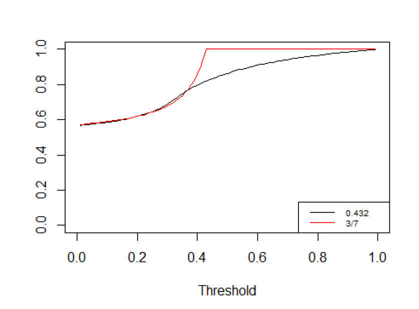
Figure 1: CDF functions of the thresholds from two random threshold algorithms

By contrast, for arbitrary randomized algorithms, it follows from Han et al. (2015) that both competitive ratios are $\frac{1}{2}$.

We now describe our techniques for establishing results 1–2 above. We first start with the following randomized algorithm, which is neither of the two algorithms described above. This algorithm flips an initial coin. With probability 2/3, the algorithm greedily accepts any item which fits in the knapsack. With probability 1/3, the algorithm accepts only the first item to have size at least 1/2 (if such an item exists).

We claim that this simple algorithm yields a constant competitiveness guarantee of 1/3. To see why, first note that if the greedy policy can fit all the items, then it is optimal, and since the algorithm is greedy with probability 2/3, it would be at least 2/3-competitive. Therefore, suppose that the greedy policy cannot fit some items, and consider two cases. If the sequence contains no items of size at least 1/2, then the greedy policy must have packed size greater than 1/2 by the time it could not fit an item, and hence the algorithm packs expected size at least $2/3\times 1/2=1/3$. In the other case, let $m$ denote the size of the first item to have size at least 1/2. When the algorithm is not greedy, it packs size $m$; and when it is greedy, it packs size at least $\min\{m,1-m\}$, which equals $1-m$ because $m\geq 1/2$. In expectation, the algorithm packs size at least

$$\frac{1}{3}m+\frac{2}{3}(1-m)=\frac{2}{3}-\frac{1}{3}m\geq\frac{1}{3}.$$

Since the algorithm in both cases packs size at least 1/3, and the optimal offline packing cannot exceed 1, this completes the claim that the algorithm is 1/3-competitive.

Now, note that the previous algorithm effectively sets a random threshold whose distribution is 0 with probability 2/3, and 1/2 with probability 1/3. To improve upon it, we consider an arbitrary distribution for the threshold $\tau$ given by the CDF $F(x)=\Pr(\tau\leq x)$, and generalize the above analysis. We now let $m$ denote the size of the smallest item which the greedy policy does not fit. In the case where $m<1/2$, we use similar arguments as above to deduce that the algorithm packs expected size at least

$$F(0)(1-m)+(F(m)-F(0))\min\{m,1-m\}.$$ (1)

However, the other case where $m\geq 1/2$ is more challenging, because when $m=1$ both terms in (1) equal 0. To refine the analysis, we define $q$ to be the maximum number such that, at the time of arrival of the item of size $m$, it would not fit even if we could “magically discard” every accepted item of size less than $q$. By the maximality of $m$, there must exist an item of size $q$. After carefully analyzing the cases (including the one where $q>m$), we show that the algorithm’s expected packing size is minimized in the case where it equals $q$ when the threshold is at most $q$, and $1-q+\varepsilon$ (for an arbitrarily small $\varepsilon>0$) when the threshold is greater than $q$. Therefore, it is lower-bounded by

$$F(q)q+(1-F(q))(1-q).$$ (2)

Finally, we solve for the maximum $c$ at which there exists a threshold distribution $F$ such that both expressions (1) and (2) exceed $c$ (for all $m$ and $q$). This turns out to be $c=3/7\approx 0.428$, and since the optimal fractional packing cannot exceed 1, the corresponding random-threshold algorithm is 0.428-competitive relative to the stronger, fractional optimum, as shown in Theorem 3.4. This competitiveness is tight relative to the stronger optimum, as shown in Theorem 3.6.

In Theorem 3.9, we improve the competitiveness to 0.432 relative to the weaker, integer optimum. The previous analysis with expressions (1) and (2) is no longer tight, because it merely lower-bounded the algorithm’s expected packing size without considering the consequences on the optimal integer packing. To improve upon the previous distribution, we perturb it to have a positive mass on all of [0,1] (instead of never setting a threshold above 3/7, as shown in Figure 1). Intuitively, this prevents the adversary from making the optimal packing size always 1 by appending a size-1 item to the end of any sequence, because if he did, then there will always be a positive probability that the algorithm sets a threshold high enough to get the size-1 item. In fact, this perturbed threshold distribution, which yields a 0.432-competitive algorithm, is best-possible for threshold algorithms relative to the optimal integer packing, as shown in Theorem 3.10.

1.3 Generalization to Static Policies for Multiple Knapsacks

We generalize to an assignment problem for multiple knapsacks, defined as follows. In this setting, there are multiple knapsacks, with potentially different capacities. An arriving item takes up a potentially different size in each knapsack, and must be irrevocably assigned to a knapsack where it fits, or outright rejected. The objective is to maximize the sum of capacities packed across all the knapsacks.

For this problem, we derive a randomized $\frac{3}{14}\approx 0.214$-competitive algorithm using a static policy which, again, does not require recording the history of past items. In particular, each item is first routed to the knapsack where it takes the greatest size (without knowing whether it would get accepted), and then an independent threshold policy at that knapsack controls whether to accept the item. This greedy routing policy is a simple implementation of threshold policies with multiple knapsacks, and is shown to be $\frac{1}{2}\times\frac{3}{7}=\frac{3}{14}$-competitive relative to the stronger optimum in Theorem 4.4, assuming that each knapsack’s threshold is chosen randomly according to the CDF which is $\frac{3}{7}$-competitive for a single knapsack. Interestingly, the CDF which improves the competitiveness to 0.432 for a single knapsack, relative to the weaker optimum, does not appear to translate to a competitiveness result for multiple knapsacks. Also, for multiple knapsacks we derive an upper bound of 0.461 on the competitive ratio for arbitrary randomized algorithms, in Theorem 4.6. This shows that the tight $\frac{1}{2}$-competitiveness for a single knapsack does not hold with multiple knapsacks, even if one could go beyond static policies.

To our knowledge, we are the first to study our generalized online assignment problem with multiple unit-density knapsacks, and derive constant-factor competitiveness results. However, our problem and results are closely related to two problems from the literature, as we outline below.

• AdWords: Our only difference from the AdWords problem studied in online advertising is that items cannot be “truncated”. That it, in AdWords, an item can be assigned to a knapsack where it exceeds the remaining capacity, and have its size “reduced” to fit the knapsack. With this truncation allowed, Mehta et al. (2005) derive a $\frac{1}{2}$-competitive algorithm in general, and a best-possible $(1-\frac{1}{e})$-competitive algorithm under the “small bids” assumption that initial capacities (“advertiser budgets”) are large compared to the sizes an item can take (“bids”).

  The competitiveness guarantee in our setting relative to the fractional optimum can only be worse than the $\frac{1}{2}$-competitiveness for AdWords, since the offline optimum is the same (being able to truncate using fractions), while the online algorithm is restricted from truncating. Our 0.214-competitive result can be seen as a weaker guarantee which holds for weaker online algorithms.

• Appointment Scheduling in Healthcare: Our only difference from the appointment scheduling problem of Stein et al. (2018) is that the sequence of items are completely unknown, instead of drawn independently from known distributions. That is, our arrival sequence can be seen as “adversarial” instead of “stochastic”. Stein et al. (2018) derive a 0.321-competitive algorithm in the stochastic setting, where the definition of competitiveness takes an expectation over the arrival sequence when evaluating both the online algorithm and the offline optimum.

  The adversarial competitive ratio can only be worse than the stochastic one. Our 0.214-competitive result can be seen as a weaker guarantee which holds in a more general setting.

Our aforementioned results, including those for a single knapsack, are summarized in Table 1.3. Note that our Theorem 4.4 also implies a $\frac{1}{4}$-competitiveness guarantee for general multi-knapsack algorithms.

Summary of lower and upper bounds on the competitive ratio, for different classes of algorithms, relative to different optima, in different settings. Results from this paper are bolded. An arrow indicates that the best-known lower (resp. upper) bound is implied by that from a more restricted (resp. less restricted) setting, pointing in the direction of that setting. Note that our paper is the only one to establish a separation between the competitiveness relative to the two different optima. Relative to Stronger Optimum Relative to Weaker Optimum Single Knapsack random-threshold algorithms [0.428 (Thm. 3.4), 0.428 (Thm. 3.6)] [0.432 (Thm. 3.9), 0.432 (Thm. 3.10)] arbitrary algorithms [0.5 (Han et al. 2015), $\longrightarrow$] [$\longleftarrow$, 0.5 (Han et al. 2015)] Multiple Knapsacks static algorithms [0.214 (Thm. 4.4), $\longrightarrow$] [$\longleftarrow$, $\downarrow$] arbitrary algorithms [0.25 (Thm. 4.4), $\longrightarrow$] [$\longleftarrow$, 0.461 (Thm. 4.6)] AdWords (truncation allowed) [0.5 (Mehta et al. 2005), $\longrightarrow$] [$\longleftarrow$, 0.632 (Karp et al. 1990)] Scheduling (stochastic arrivals) [0.321 (Stein et al. 2018), $\longrightarrow$] [$\longleftarrow$, 0.5 (Stein et al. 2018)]

1.4 Simulations Using Supply Chain Data of A Latin American Chain Department Store

We now describe how our optimal random-threshold distributions for a single knapsack can be implemented across the supply chain of our industry partner, a Latin American chain department store. They sell 974 SKU’s in the young women’s fashion category. There are 21 warehouses, and every SKU is stored in a subset of different warehouses. Every (SKU, warehouse)-pair faces a stream of orders, each for a specific number of units. Orders cannot be split or redirected to a different warehouse, so order sizes greater than the available inventory must be rejected. Therefore, our industry partner faces the same accept/reject problem on order sizes, and has the same goal of maximizing total inventory fulfilled, equal to the sum of sizes of accepted orders.

The data we observe is the sizes of all orders accepted by a greedy First-Come-First-Serve (FCFS) policy. The sum of all observed order sizes for each of our (SKU, warehouse)-pairs is then at most the starting inventory, since the order sizes that cannot be fulfilled have been censored. To create non-trivial instances, we re-scale the starting inventory amounts (which we know) for each SKU at each warehouse by a factor $\alpha\in[0,1]$, and test the performance of different accept/reject policies over different scaling factors $\alpha$.

To implement our random-threshold policies, we take 21 evenly-spaced percentiles of the threshold distribution $F$, that is, we take the 21 thresholds defined by $F^{-1}(0),F^{-1}(0.05),...,F^{-1}(0.95),F^{-1}(1)$. Then we assign them (i.e. randomly permute them) over the 21 warehouses, making accept/reject decisions at each warehouse based on the assigned threshold (scaled by the starting inventory). We believe this assignment of percentiles to warehouses is how our threshold distribution $F$ would be implemented in practice. We then average the fulfillment ratios over the warehouses to determine the performance for a specific SKU. We take an outer average over many independent random permutations of warehouses to define a final performance ratio for each of the 974 SKU’s.

We find that the greedy FCFS policy has the best average-case performance ratio, even when the scaling factor $\alpha$ for initial inventory is small. While this is discouraging, we believe that the way in which order sizes are censored in our data favors FCFS, since large orders cannot come at the end. Nonetheless, for any $\alpha$, if we look at the worst-case SKU, then our random-threshold policy has the best performance. Indeed, the way in which it distributes different thresholds over the warehouses provides a form of “hedging” for each SKU, and our random-threshold policy being robust to the worst case is consistent with it having the best competitive ratio. This robustness is not achieved by FCFS, the algorithm of Han et al. (2015), or even any deterministic-threshold algorithm.

1.5 Other Related Work and Applications

To the best of our knowledge, we are the first to use threshold policies to study the competitive ratios of randomized algorithms for this foundational unit-density online knapsack problem. Without the unit-density assumption, the non-existence of any constant competitive ratio guarantee $c>0$, even for randomized algorithms on a single knapsack, was first established in Marchetti-Spaccamela and Vercellis (1995). Tight instance-dependent competitive ratios (where the guarantee $c$ can depend on parameters based on the sequence of items) have also been established in Zhou et al. (2008). For a thorough discussion of recent results across many variants online knapsack, we refer to Cygan et al. (2016).

There is also a rich literature which studies the stochastic online knapsack problem, that assumes the arrival sequences are drawn from a given distribution. There are papers on the optimal policies on a single knapsack; see Kleywegt and Papastavrou (1998), Papastavrou et al. (1996) when the order of arriving items is fixed. When the items can be inserted in any order but their sizes are stochastic, the concept of “adaptivity gap” between adaptive and non-adaptive algorithms was proposed in Dean et al. (2008). Using their language, the adaptivity gap for our problem on a single knapsack is within $7\%$; see Table 1.3. Variants where the arrival sequence could be (partially) learned over time are studied in Modaresi et al. (2019), Hwang et al. (2018).

We briefly mention some other applications areas (other than Adwords and healthcare scheduling) where online knapsack/assignment problems with unit density and no truncation arise.

Refugee Integration: Bansak et al. (2018) have studied a refugee integration problem. This is a real problem in many developed democracies, where “refugees face challenges integrating into host societies”. Refugees in non-splittable groups (e.g. families) arrive in an online fashion, and democracies assign refugees across resettlement locations subject to capacity constraints. If a group of refugees do not have a suitable settlement location, they temporarily stay in the refugee camps. The objective is to maximize the number of assigned refugees.

Crowdsourcing: Ho and Vaughan (2012) have studied a problem in online crowdsourcing, where a requester asks workers that arrive online to finish his / her tasks, and cannot split tasks into two. Each worker spends some time to finish the assigned work. The objective is to maximize the total benefit that the requester obtains from the completed work, given time constraints. In a variant (Assadi et al. 2015), each worker picks a subset of tasks, along with task-specific bid numbers. The requester has to assign no more than one task to each worker, by paying the worker the on the bid. The objective of the requester is to either maximize the number of assigned tasks to workers, while not violating the budget constraint.

1.6 Roadmap

In Section 2 we introduce the model and notations. In Section 3 we introduce our results on a single knapsack. Section 3.1 introduces the $3/7$ competitive algorithm relative to the optimal fractional packing, and Section 3.2 introduces the $0.432$ competitive algorithm relative to the optimal integer packing. Then in Section 4 we introduce our results on multiple knapsacks. Section 4.1 introduces the $0.214$ competitive algorithm, and Section 4.2 introduces the impossibility result for a $0.461$ competitive algorithm. Finally in Section 5, we conduct computational study using real data from a Latin American chain department Store, and show the efficacy of threshold algorithms.

2 Definition of Problems, Notations

In this paper we denote $[T]=\{1,2,...,T\}$, for any positive integer $T$. Let the capacity of the knapsack be $1$. Let the entire set of items be indexed by $t\in[T]$, the sequence of its arrival. For any $t\in[T],s_{t}$ refers to the size of item $t$. The entire sequence of item sizes is then $S=(s_{1},s_{2},...,s_{T})$. For any $A\subseteq[T]$, a subset of indices, let $\mathsf{size}(A)=\sum_{t\in A}s_{t}$ be the total size of items in $A$.

Suppose there is a clairvoyant decision maker who knows the entire sequence in advance. This decision maker is going to take the optimal actions (accept / reject) over the process. Let this policy be $\mathsf{OPT}$. Note that $\mathsf{OPT}$ does not necessarily guarantee to fill all the capacity of the knapsack, but it must be upper bounded by $1$.

For any specific sequence of $S$, let $\mathsf{ALG}(S)$ denote the total amount filled by $\mathsf{ALG}$ on this instance in expectation, where expectation is taken over the randomness of the algorithm. Here $\mathsf{ALG}$ is any generic algorithm, where in the following sections we will specify which algorithm it is by using slightly different notations for each algorithm. Let $\mathsf{OPT}(S)$ denote the total amount filled by $\mathsf{OPT}$ on this sequence. Note that $\mathsf{OPT}(S)=\max_{A\subseteq[T]:\mathsf{size}(A)\leq 1}\mathsf{size}(A)$. We will also refer to a stronger optimum $\mathsf{OPT}^{+}$ which is not only clairvoyant, but allowed to truncate items at will, with

$$\mathsf{OPT}^{+}(S)=\min\{s_{1}+\cdots+s_{T},1\}$$ (3)

It is self-evident that $\mathsf{OPT}(S)\leq\mathsf{OPT}^{+}(S)$ for any $S$. We also use $\mathsf{ALG},\mathsf{OPT}$ and $\mathsf{OPT}^{+}$ for $\mathsf{ALG}(S),\mathsf{OPT}(S)$, and $\mathsf{OPT}^{+}(S)$, respectively, if the sequence $S$ is clear from the context.

Under any policy, we say that an item $s_{t}$ is rejected because it fails to meet the admission critrion of this policy, e.g. failure to exceed the threshold of a threshold policy. If an item is rejected under a policy, we say that this policy rejects this item.

Under any policy, we say that an item $s_{t}$ is blocked at the moment it arrives, if the remaining capacity of the knapsack is not enough for $s_{t}$ to fit in. An item is said to be blocked regardless of the fact if it would have been rejected by the policy. If an item is blocked under a policy, we say that this policy blocks this item.

The focus of this paper is on randomized (non-adaptive) threshold algorithms.

We define threshold algorithms as follows: Let $\mathsf{THR}(\tau),\forall\tau\in[0,1]$ be a threshold algorithm that accepts any item whose size is greater or equal to $\tau$, as long as it can fit into the knapsack. A $\mathsf{THR}(0)$ policy is also referred to as a greedy policy, $\mathsf{Greedy}$: accept any item regardless of its size, as long as it can fit into the knapsack. We will interchangeably use $\mathsf{THR}(0)$ and $\mathsf{Greedy}$ for the same policy.

We say that threshold algorithms are non-adaptive, because the decision of whether to accept an item (assuming it fits) is dependent on only the item’s size, and not the past items observed. Note that a threshold algorithm can be randomized, in which case $\tau$ is chosen from a probability distribution at the start and then fixed over time.

3 A Single Knapsack

We first start with a single knapsack. We introduce the algorithm from Han et al. (2015) here.

Definition 3.1

[Algorithm $\mathsf{TwoBins}$, Han et al. (2015)]

1. Randomly flip a fair coin, with probability $1/2$ on each side.

2. If Heads, apply $\mathsf{Greedy}$.

3. If Tails, reject everything until the first one that $\mathsf{Greedy}$ would have not fit. Then apply $\mathsf{Greedy}$ (including this item).

Note that when Tails, the algorithm has to adapt on what are the items that have been rejected. So unlike our algorithms, this is an adaptive algorithm. Nonetheless, it provides the best possible competitive ratio.

Proposition 3.2 (Theorem 1, Han et al. (2015))

The algorithm from Definition 3.1 is $1/2$ competitive, and it is tight for any algorithm, i.e. $\forall S$,

$$\inf_{S}\frac{\mathsf{TwoBin}(S)}{\mathsf{OPT}^{+}(S)}=\frac{1}{2}.$$

The proof is very simple, as we outlined in the Introduction. Either greedy is optimal, in which case the algorithm is optimal half the time, or the sum of the algorithm’s packing under Heads and Tails exceeds 1, in which case the algorithm’s expected packing must be at least half of the optimum.

Next, in Section 3.1, we prove a tight $3/7$ competitive ratio relative to the optimal fractional packing, in the family of non-adaptive threshold algorithms, by lower bounding the performance of our proposed algorithm and loosely upper bounding the optimal fractional packing by $1$. In Section 3.2, we prove a tight $0.432$ competitive ratio relative to the optimal integer packing, in the family of non-adaptive threshold algorithms, by lower bounding the performance of our proposed algorithm and upper bounding the exact optimal integer packing at the same time.

3.1 A 0.428 Competitive Algorithm Relative to the Optimal Fractional Packing

We propose a randomized threshold policy, $\mathsf{ALG}_{\mathsf{N\ref{defn:3/7alg}}}$, and prove it is $3/7$-competitive.

Definition 3.3

Let $\mathsf{ALG}_{\mathsf{N\ref{defn:3/7alg}}}$ be a randomized threshold policy that runs as follows,

1. At the beginning of the entire process, randomly draw $\tau$ from a distribution whose cumulative distribution function (CDF) is given by

   $$F_{\textit{N\ref{defn:3/7alg}}}(x)=\left\{\begin{aligned} &\frac{4/7-x}{1-2x},&\quad x\in[0,3/7]\\ &1,&\quad x\in(3/7,1]\end{aligned}\right.$$ (4)

2. We apply $\mathsf{THR}(\tau)$ policy throughout the process.

Notice that $F_{\textit{N\ref{defn:3/7alg}}}(0)=4/7$. This is the point mass we put on $\tau=0$. This means that with probability $4/7$, we will perform $\mathsf{Greedy}$.

It is easy to check that our desired algorithm does not know how many items are there in total, not does it know the sizes of the items.

Now we state and prove our first result.

Theorem 3.4

$$\inf_{S}\frac{\mathsf{ALG}_{\mathsf{N\ref{defn:3/7alg}}}(S)}{\mathsf{OPT}^{+}(S)}\geq\frac{3}{7}$$

Proof 3.5

Proof of Theorem 3.4. For any instance of arrival sequence $S$, we will show $\frac{\mathsf{ALG}_{\mathsf{N\ref{defn:3/7alg}}}(S)}{\mathsf{OPT}^{+}(S)}\geq 3/7$.

First of all, $\mathsf{Greedy}$ always accepts something. Denote the set of items accepted by $\mathsf{Greedy}$ as $G$. Denote $\left|G\right|=g$. If $G=[T]$ then $\mathsf{Greedy}$ is optimal. In this case

$$\frac{\mathsf{ALG}_{\mathsf{N\ref{defn:3/7alg}}}}{\mathsf{OPT}^{+}}\geq\Pr(\tau=0)\cdot 1+\Pr(\tau>0)\cdot 0\geq F(0)=4/7\geq 3/7.$$

If $G\subsetneqq[T]$, let $M=[T]\backslash G$ denote the set of items blocked by $\mathsf{Greedy}$. Since $\mathsf{Greedy}$ always accepts an item as long as it can fill in, any item blocked by $\mathsf{Greedy}$ must exceed the remaining space of the knapsack, at the moment it is blocked. We also know that $G\cup M=[T]$, $G\cap M=\phi$.

Let $m$ be the smallest size in $M$, i.e. $m=\min_{t\in M}s_{t}$. Define index $t_{m}$ for the smallest item, or the first smallest item, if there are multiple smallest items.

$$t_{m}=\min\left\{t\in[T]\left|s_{t}=m\right.\right\}.$$ (5)

Denote $G^{\prime}$ as the set of items accepted by $\mathsf{Greedy}$, at the moment item $t_{m}$ is blocked. Let $g^{\prime}=\mathsf{size}(G^{\prime})$. See Figure 2. A straightforward, but useful information about $m$ is:

$$g^{\prime}+m>1,$$ (6)

because $m$ is blocked by $\mathsf{Greedy}$. We wish to understand when we can pack an item of size at least $m$, by selecting a proper threshold $\tau$.

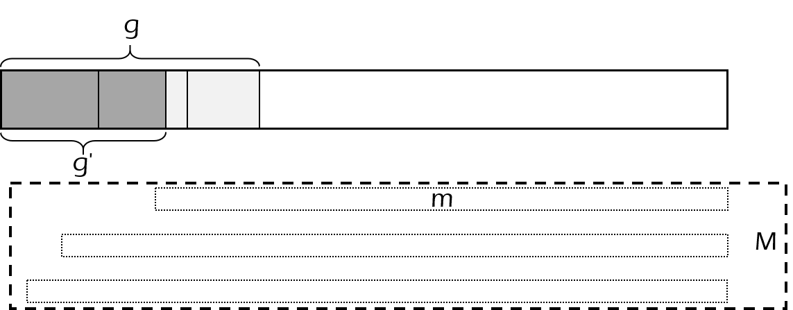
Figure 2: Illustration of the items that $\mathsf{Greedy}$ accepts, and blocks

We distinguish two cases: $m\geq 1/2$ and $m<1/2$.

Case 1: $m\geq 1/2$.
Let $S^{\mathsf{THR}}(\tau)$ be the set of items that have sizes at least $\tau$, i.e. $S^{\mathsf{THR}}(\tau)=\left\{t\in S\left|s_{t}\geq\tau\right.\right\}$. Now define

$$\begin{split}q=\max&\quad\tau\\ s.t.&\quad m+\mathsf{size}(S^{\mathsf{THR}}(\tau)\cap G^{\prime})>1\end{split}$$ (7)

This means that if we adopt a $\mathsf{THR}(q)$ policy, then the size $m$ item must be blocked (possibly it will also be rejected, due to $q>m$, which leads to the discussion in Case 1.1).

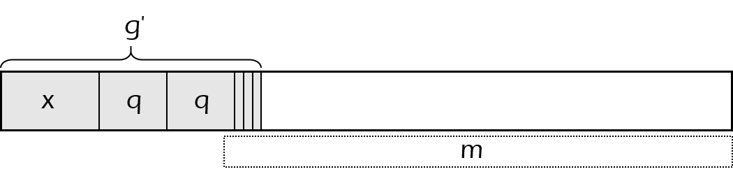
Figure 3: Illustration of Case 1 (and specifically, Case 1.2)

Now consider the items in $S^{\mathsf{THR}}(q)\cap G^{\prime}$. These items have sizes at least $q$. We count how many size $q$ items are there, and let $n$ be the number of size $q$ items. Denote the total size of the remaining items be $x$. We know that $\mathsf{size}(S^{\mathsf{THR}}(q)\cap G^{\prime})=nq+x$. See Figure 3.

We make the following observations:

1. There must exist some item from $G^{\prime}$ that is of size $q$, i.e.

   $$\exists t_{q}\in G^{\prime}\subseteq[T],s.t.\ s_{t_{q}}=q.$$ (8)

   This is because otherwise we can select the smallest item size in $G^{\prime}$ that is also larger than $q$. This item size satisfies (7), and violates the maximum property of $q$.

2. Size $m$ items can not fit in together with all the items in $S^{\mathsf{THR}}(q)\cap G^{\prime}$, i.e.

   $$nq+x+m>1$$ (9)

   This is because $\mathsf{size}(S^{\mathsf{THR}}(q)\cap G^{\prime})=nq+x$. This is implied by (7).

3. A size $m$ item can fit in together with items $S^{\mathsf{THR}}(\tau)\cap G^{\prime},\forall\tau>q$, i.e.

   $$x+m\leq 1$$ (10)

   This is because otherwise we could further increase $q$ to $\hat{q}$, so that $\hat{q}$ still satisfy equation (7). Define $\hat{q}=\min_{\varepsilon>0,t\in S^{\mathsf{THR}}(q+\varepsilon)\cap G^{\prime}}s_{t}$. We know (i) $\hat{q}>q$; (ii) $\mathsf{size}(S^{\mathsf{THR}}(\hat{q})\cap G^{\prime})+m>1$. So $\hat{q}$ violates the maximum property of $q$.

We further distinguish two cases: $q>m$, and $q\leq m$.

Case 1.1: $q>m$.
In this case, if we adopt $\mathsf{Greedy}$ then we can get as much as $g$.

If we adopt $\mathsf{THR}(\tau),\forall\tau\in(0,q]$ then we can get no less than $q$. This is because due to (8) there must exist some item $t_{q}\in G^{\prime}$ of size $q$. We either accept it, in which case we immediately earn $q$, or we have blocked it because we admitted some item $z\in[T]$ from $M$ and consumed too much space. But $\mathsf{Greedy}$ blocks item $z$ earlier than it accepts item $t_{q}$, which means that $s_{z}\geq s_{t_{q}}=q$. So in either case we earn $q$.

We have the following:

$$\mathsf{ALG}_{\mathsf{N\ref{defn:3/7alg}}} \geq\Pr(\tau=0)\cdot g+\Pr(0<\tau\leq q)\cdot q$$

$$=F_{\textit{N\ref{defn:3/7alg}}}(0)\cdot g+(F_{\textit{N\ref{defn:3/7alg}}}(q)-F_{\textit{N\ref{defn:3/7alg}}}(0))\cdot q$$

$$\geq F_{\textit{N\ref{defn:3/7alg}}}(0)\cdot(1-2q)+F_{\textit{N\ref{defn:3/7alg}}}(q)\cdot q$$

$$=4/7\cdot(1-2q)+1\cdot q$$

$$=4/7-1/7\cdot q$$

$$\geq 3/7$$

where the second inequality is because $g\geq g^{\prime}>1-m$ (due to (6)) and $1-m>1-q$ (Case 1.1: $q>m$); second equality is because $q>m\geq 1/2$ and the way we defined $F_{\textit{N\ref{defn:3/7alg}}}(\cdot)$ in (4) so $F_{\textit{N\ref{defn:3/7alg}}}(q)=1$; last inequality is because $q\leq 1$.

Since $\mathsf{OPT}^{+}\leq 1$, we have $\frac{\mathsf{ALG}_{\mathsf{N\ref{defn:3/7alg}}}}{\mathsf{OPT}^{+}}\geq\frac{3}{7}$.

Case 1.2: $q\leq m$.
In this case, if we adopt $\mathsf{Greedy}$ then we can get as much as $g$. This is the definition of $g$.

If we adopt $\mathsf{THR}(\tau),\forall\tau\in(0,q]$ then we get no less than $q$. This is because due to (8) there must exist some item $t_{q}\in G^{\prime}$ of size $q$. We either accept it, in which case we immediately earn $q$, or we have blocked it because we admitted some item $z\in[T]$ from $M$ and consumed too much space. But $\mathsf{Greedy}$ blocks item $z$ earlier than it accepts item $t_{q}$, which means that $s_{z}\geq s_{t_{q}}=q$. So in either case we earn $q$.

If we adopt $\mathsf{THR}(\tau),\forall\tau\in(q,m]$ then we get no less than $m$. This is because due to (10), any item in $S^{\mathsf{THR}}(\tau)\cap G^{\prime}$ will not block item $t_{m}$ (from expression (5)); and $\tau\leq m$ so we will not reject item $t_{m}$. We either accept item $t_{m}$, in which case we immediately earn $m$, or we have blocked it because we admitted some item $z\in[T]$ from M and consumed too much space. But $m$ is smallest item size in $M$, which means that $s_{z}\geq m$. So in either case we earn $m$.

We have the following:

$$\mathsf{ALG}_{\mathsf{N\ref{defn:3/7alg}}} \geq\Pr(\tau=0)\cdot g+\Pr(0<\tau\leq q)\cdot q+\Pr(q<\tau\leq m)\cdot m$$

$$=F_{\textit{N\ref{defn:3/7alg}}}(0)\cdot g+(F_{\textit{N\ref{defn:3/7alg}}}(q)-F_{\textit{N\ref{defn:3/7alg}}}(0))\cdot q+(F_{\textit{N\ref{defn:3/7alg}}}(m)-F_{\textit{N\ref{defn:3/7alg}}}(q))\cdot m$$

$$\geq F_{\textit{N\ref{defn:3/7alg}}}(0)\cdot(nq+x)+(F_{\textit{N\ref{defn:3/7alg}}}(q)-F_{\textit{N\ref{defn:3/7alg}}}(0))\cdot q+(F_{\textit{N\ref{defn:3/7alg}}}(m)-F_{\textit{N\ref{defn:3/7alg}}}(q))\cdot(1-(nq+x))$$

$$=(F_{\textit{N\ref{defn:3/7alg}}}(q)-F_{\textit{N\ref{defn:3/7alg}}}(0))\cdot q+1-F_{\textit{N\ref{defn:3/7alg}}}(q)+(F_{\textit{N\ref{defn:3/7alg}}}(q)-3/7)\cdot(nq+x)$$

$$\geq(F_{\textit{N\ref{defn:3/7alg}}}(q)-F_{\textit{N\ref{defn:3/7alg}}}(0))\cdot q+1-F_{\textit{N\ref{defn:3/7alg}}}(q)+(F_{\textit{N\ref{defn:3/7alg}}}(q)-3/7)\cdot q$$

$$=F_{\textit{N\ref{defn:3/7alg}}}(q)\cdot(2q-1)+1-q$$

where the second inequality is because $g\geq g^{\prime}\geq nq+x$ and $m>1-(nq+x)$ (due to (9)); second equality is because $m\geq 1/2$ and the way we defined $F_{\textit{N\ref{defn:3/7alg}}}(\cdot)$ in (4) so $F_{\textit{N\ref{defn:3/7alg}}}(m)=1$; the last inequality is because $F_{\textit{N\ref{defn:3/7alg}}}(q)\geq F_{\textit{N\ref{defn:3/7alg}}}(0)=4/7>3/7$, so the coefficient in front of $nq+x$ is positive.

Now we plug in the expression of $F_{\textit{N\ref{defn:3/7alg}}}(q)$ as defined in (4). If $q\leq 3/7$ then $\mathsf{ALG}_{\mathsf{N\ref{defn:3/7alg}}}\geq\frac{4/7-q}{1-2q}\cdot(2q-1)+1-q=3/7;$ If $q>3/7$ then $\mathsf{ALG}_{\mathsf{N\ref{defn:3/7alg}}}\geq q>3/7.$ So in either case we have shown $\mathsf{ALG}_{\mathsf{N\ref{defn:3/7alg}}}\geq 3/7$.

Since $\mathsf{OPT}^{+}\leq 1$, we have $\frac{\mathsf{ALG}_{\mathsf{N\ref{defn:3/7alg}}}}{\mathsf{OPT}^{+}}\geq\frac{3}{7}$.

Case 2: $m<1/2$.
In this case, a crude analysis is enough. See Figure 4.

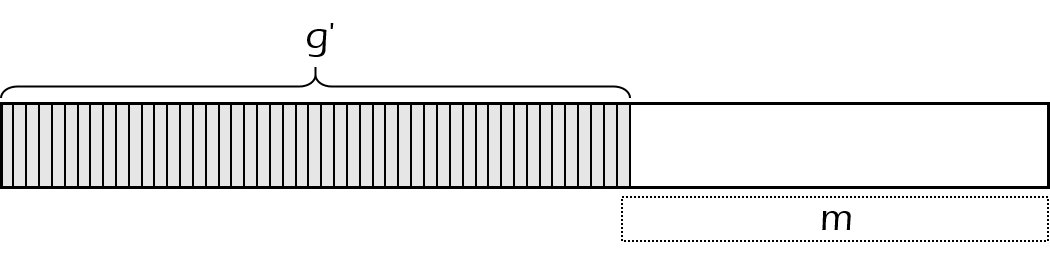
Figure 4: Illustration of Case 2

If we adopt $\mathsf{Greedy}$ then we can get as much as $g$. This is because $g$ is defined this way.

If we adopt $\mathsf{THR}(\tau),\forall\tau\in(0,m]$ then we either get $m$, or $m$ is blocked, in which case we must have already earned at least $1-m$ to block $m$.

We have the following:

$$\mathsf{ALG}_{\mathsf{N\ref{defn:3/7alg}}} \geq\Pr(\tau=0)\cdot g+\Pr(0<\tau\leq m)\cdot\min\{m,1-m\}$$

$$\geq\Pr(\tau=0)\cdot g+\Pr(0<\tau\leq m)\cdot m$$

$$=F_{\textit{N\ref{defn:3/7alg}}}(0)\cdot g+(F_{\textit{N\ref{defn:3/7alg}}}(m)-F_{\textit{N\ref{defn:3/7alg}}}(0))\cdot m$$

$$\geq F_{\textit{N\ref{defn:3/7alg}}}(0)\cdot(1-m)+(F_{\textit{N\ref{defn:3/7alg}}}(m)-F_{\textit{N\ref{defn:3/7alg}}}(0))\cdot m$$

$$=F_{\textit{N\ref{defn:3/7alg}}}(m)\cdot m+4/7\cdot(1-2m)$$

where the second inequality is because $m<1/2$; the last inequality is because $g\geq g^{\prime}>1-m$ (due to (6)).

Now we plug in the expression of $F_{\textit{N\ref{defn:3/7alg}}}(m)$ as defined in (4). If $m>3/7$ then $\mathsf{ALG}_{\mathsf{N\ref{defn:3/7alg}}}\geq 4/7-1/7\cdot m\geq 3/7$, because $m<1/2\leq 1$; If $m\leq 3/7$ then

$$\mathsf{ALG}_{\mathsf{N\ref{defn:3/7alg}}}\geq\frac{4/7-m}{1-2m}\cdot m+\frac{4}{7}\cdot(1-2m)=\frac{9}{28}\cdot(1-2m)+\frac{1}{28}\cdot\frac{1}{1-2m}+\frac{3}{14}\geq 2\sqrt{\frac{9}{28}\cdot\frac{1}{28}}+\frac{3}{14}=\frac{3}{7}.$$

So in either case we have $\mathsf{ALG}_{\mathsf{N\ref{defn:3/7alg}}}\geq 3/7$.

Since $\mathsf{OPT}^{+}\leq 1$, we have $\frac{\mathsf{ALG}_{\mathsf{N\ref{defn:3/7alg}}}}{\mathsf{OPT}^{+}}\geq\frac{3}{7}$.

In all, we have enumerated all the possible cases, to find $\dfrac{\mathsf{ALG}_{\mathsf{N\ref{defn:3/7alg}}}}{\mathsf{OPT}^{+}}\geq\dfrac{3}{7}$ always holds.

3.1.1 Tightness proof of the $3/7$ competitive algorithm.

In this section we show that the guarantee of $\inf_{S}\frac{\mathsf{ALG}_{\mathsf{N\ref{defn:3/7alg}}}(S)}{\mathsf{OPT}^{+}(S)}\geq\frac{3}{7}$ from Definition 3.3 is best-possible, relative to $\mathsf{OPT}^{+}$, among all randomized threshold policies. To do this, we invoke the minimax theorem of Yao (1977), which says that it suffices to construct a distribution $\mathcal{S}$ over sequences $S$ for which

$$\sup_{\mathsf{ALG}:\mathsf{ALG}=\mathsf{THR}(\tau),\tau\in[0,1]}\frac{\mathbb{E}_{S\sim\mathcal{S}}[\mathsf{ALG}(S)]}{\mathbb{E}_{S\sim\mathcal{S}}[\mathsf{OPT}^{+}(S)]}\leq\frac{3}{7}.$$

In particular, we only need to establish that $\frac{\mathbb{E}_{S\sim\mathcal{S}}[\mathsf{ALG}(S)]}{\mathbb{E}_{S\sim\mathcal{S}}[\mathsf{OPT}^{+}(S)]}\leq\frac{3}{7}$ for deterministic threshold policies specified by a $\tau\in[0,1]$.

Theorem 3.6

There exists a distribution $\mathcal{S}$ over arrival sequences $S$ such that for any $\tau\in[0,1]$, the algorithm $\mathsf{ALG}=\mathsf{THR}(\tau)$ has $\frac{\mathbb{E}_{S\sim\mathcal{S}}[\mathsf{ALG}(S)]}{\mathbb{E}_{S\sim\mathcal{S}}[\mathsf{OPT}^{+}(S)]}\leq\frac{3}{7}.$

Proof 3.7

Proof of Theorem 3.6. Prove by construction. Let the random arrival sequence be $S$:

$$S=\left\{\begin{aligned} &(1/3,2/3+\varepsilon),&&\text{with prob. }3/7;\\ &(\underbrace{\varepsilon,\varepsilon,...,\varepsilon}_{2/3+\varepsilon},1/3),&&\text{with prob. }3/7;\\ &(\varepsilon,1),&&\text{with prob. }1/7;\end{aligned}\right.$$ (11)

Following each realization of $S$, $\mathsf{OPT}^{+}(S)=1$. So we have $\mathbb{E}_{S}[\mathsf{OPT}^{+}(S)]=1$.

For any $\mathsf{ALG}=\mathsf{THR}(\tau),\tau\in[0,1]$, we enumerate all the potential values of $\tau$ in the following.
Case 1: $0\leq\tau\leq\varepsilon$. In this case,

$$\mathbb{E}_{S}[\mathsf{ALG}(S)]=\frac{1}{3}\cdot\frac{3}{7}+\left(\frac{2}{3}+\varepsilon\right)\cdot\frac{3}{7}+\varepsilon\cdot\frac{1}{7}=\frac{3}{7}+\frac{4}{7}\cdot\varepsilon$$

Case 2: $\varepsilon<\tau\leq 1/3$. In this case,

$$\mathbb{E}_{S}[\mathsf{ALG}(S)]=\frac{1}{3}\cdot\frac{3}{7}+\frac{1}{3}\cdot\frac{3}{7}+1\cdot\frac{1}{7}=\frac{3}{7}$$

Case 3: $1/3<\tau\leq 2/3+\varepsilon$. In this case,

$$\mathbb{E}_{S}[\mathsf{ALG}(S)]=\left(\frac{2}{3}+\varepsilon\right)\cdot\frac{3}{7}+0\cdot\frac{3}{7}+1\cdot\frac{1}{7}=\frac{3}{7}+\frac{3}{7}\cdot\varepsilon$$

Case 4: $2/3+\varepsilon<\tau\leq 1$. In this case,

$$\mathbb{E}_{S}[\mathsf{ALG}(S)]=1\cdot\frac{1}{7}=\frac{1}{7}$$

In all, we have enumerated all the values that a threshold can take. In all cases, the performance of the threshold $\mathsf{THR}(\tau)$ policy has an expected performance of no more than $3/7+4/7\cdot\varepsilon$. But $\mathbb{E}_{S}[\mathsf{OPT}^{+}(S)]=1$. By taking $\varepsilon\to 0^{+}$ we finish the proof.

3.2 A 0.432 Competitive Algorithm Relative to the Optimal Integer Packing

In this section we are going to introduce a threshold policy that achieves the best-possible competitive ratio in the non-adaptive threshold family. In Section 3.2.1 we will show it is best-possible.

We first define some parameters that are going to be useful in the following analysis.

Let $H:[3/7,1/2)\times(0,1/2)\to\mathrm{R}_{+}$ be a bivariate real function defined as follows:

$$H(c,x)=\frac{1-2c}{x}-\frac{(1-2c)\ln{(1-x)}}{1-2x}-(1-c)$$

Now fix $c$ to be any number between $[3/7,1/2)$. Define $q_{\textit{N\ref{defn:0.432alg}}}$ to be the only local minimizer on the second coordinate of $H(c,x)$, between $(0,1/2)$ – it can be implicitly given as the only solution between $[3/7,1/2)$, such that

$$2q_{\textit{N\ref{defn:0.432alg}}}^{3}-7q_{\textit{N\ref{defn:0.432alg}}}^{2}+5q_{\textit{N\ref{defn:0.432alg}}}-1-2(1-q_{\textit{N\ref{defn:0.432alg}}})q_{\textit{N\ref{defn:0.432alg}}}^{2}\ln{(1-q_{\textit{N\ref{defn:0.432alg}}})}=0,$$

or, approximately,

$$q_{\textit{N\ref{defn:0.432alg}}}\approx 0.31847.$$

Define $c_{\textit{N\ref{defn:0.432alg}}}$ to be the only solution between $[3/7,1/2)$, such that

$$H(c_{\textit{N\ref{defn:0.432alg}}},q_{\textit{N\ref{defn:0.432alg}}})=\frac{1-2c_{\textit{N\ref{defn:0.432alg}}}}{q_{\textit{N\ref{defn:0.432alg}}}}-\frac{(1-2c_{\textit{N\ref{defn:0.432alg}}})\ln{(1-q_{\textit{N\ref{defn:0.432alg}}})}}{1-2q_{\textit{N\ref{defn:0.432alg}}}}-(1-c_{\textit{N\ref{defn:0.432alg}}})=0,$$ (12)

or, approximately,

$$c_{\textit{N\ref{defn:0.432alg}}}\approx 0.43236.$$

We can check the following inequality: $\forall q\in(0,1/2)$,

$$H(c_{\textit{N\ref{defn:0.432alg}}},q)\geq H(c_{\textit{N\ref{defn:0.432alg}}},q_{\textit{N\ref{defn:0.432alg}}})=0$$ (13)

We propose another randomized threshold policy, $\mathsf{ALG}_{\mathsf{N\ref{defn:0.432alg}}}$, using another random threshold. It gives us an improved $0.432$ competitive guarantee.

Definition 3.8

Let $\mathsf{ALG}_{\mathsf{N\ref{defn:0.432alg}}}$ be a randomized threshold policy that runs as follows,

1. At the beginning of the entire process, randomly draw $\tau$ from a distribution whose CDF is given by

   $$F_{\textit{N\ref{defn:0.432alg}}}(x)=\left\{\begin{aligned} &(1-c_{\textit{N\ref{defn:0.432alg}}})-\frac{(1-2c_{\textit{N\ref{defn:0.432alg}}})\ln{(1-x)}}{1-2x},&x\in[0,q_{\textit{N\ref{defn:0.432alg}}}]\\ &2(1-c_{\textit{N\ref{defn:0.432alg}}})-\frac{1-2c_{\textit{N\ref{defn:0.432alg}}}}{x},&x\in(q_{\textit{N\ref{defn:0.432alg}}},1]\end{aligned}\right.$$ (14)

2. We apply $\mathsf{THR}(\tau)$ policy throughout the process.

Notice that $F_{\textit{N\ref{defn:0.432alg}}}(0)=1-c_{\textit{N\ref{defn:0.432alg}}}$. This is the point mass we put on $\tau=0$. This means that with probability $1-c_{\textit{N\ref{defn:0.432alg}}}\approx 0.568$, we will perform $\mathsf{Greedy}$.

We state our main result here.

Theorem 3.9

$$\inf_{S}\frac{\mathsf{ALG}_{\mathsf{N\ref{defn:0.432alg}}}(S)}{\mathsf{OPT}(S)}\geq c_{\textit{N\ref{defn:0.432alg}}}\approx 0.432$$

The proof idea is the same as in Theorem 3.4, but in order to improve it, we are more careful in upper bounding the performance of $\mathsf{OPT}$. To compare to the proof of Theorem 3.4, Case 1.2 will be different. The proof details are deferred to Section 7.

3.2.1 Tightness proof of the $0.432$ competitive algorithm.

In this section we show that the guarantee of $\inf_{S}\frac{\mathsf{ALG}(S)}{\mathsf{OPT}(S)}\geq c_{\textit{N\ref{defn:0.432alg}}}$ from Definition 3.8 is best-possible among all randomized threshold policies. As in Section 3.1.1, we invoke the minimax theorem of Yao (1977), which says that it suffices to construct a distribution $\mathcal{S}$ over sequences $S$ for which

$$\sup_{\mathsf{ALG}:\mathsf{ALG}=\mathsf{THR}(\tau),\tau\in[0,1]}\frac{\mathbb{E}_{S\sim\mathcal{S}}[\mathsf{ALG}(S)]}{\mathbb{E}_{S\sim\mathcal{S}}[\mathsf{OPT}(S)]}\leq c_{\textit{N\ref{defn:0.432alg}}}.$$

Theorem 3.10

There exists a distribution $\mathcal{S}$ over arrival sequences $S$ such that for any $\tau\in[0,1]$, the algorithm $\mathsf{ALG}=\mathsf{THR}(\tau)$ has $\frac{\mathbb{E}_{S\sim\mathcal{S}}[\mathsf{ALG}(S)]}{\mathbb{E}_{S\sim\mathcal{S}}[\mathsf{OPT}(S)]}\leq c_{\textit{N\ref{defn:0.432alg}}}\approx 0.432.$

Proof 3.11

Proof of Theorem 3.10. Prove by construction. Let the random arrival sequence be $S$:

$$S=\left\{\begin{aligned} &(\underbrace{\varepsilon,\varepsilon,...,\varepsilon}_{1-q+\varepsilon},q),&&\text{where }q\in[1-q_{\textit{N\ref{defn:0.432alg}}},1]\text{ conforms }u(\cdot);\\ &(q_{\textit{N\ref{defn:0.432alg}}},1-q_{\textit{N\ref{defn:0.432alg}}}+\varepsilon,1-q_{\textit{N\ref{defn:0.432alg}}}+2\varepsilon,...,1),&&\text{with prob. }x;\\ &(\underbrace{\varepsilon,\varepsilon,...,\varepsilon}_{1-q_{\textit{N\ref{defn:0.432alg}}}+\varepsilon},q_{\textit{N\ref{defn:0.432alg}}}),&&\text{with prob. }y;\\ &(\varepsilon,1),&&\text{with prob. }z;\end{aligned}\right.$$ (15)

where

$$x=\frac{1-2c_{\textit{N\ref{defn:0.432alg}}}}{1-2q_{\textit{N\ref{defn:0.432alg}}}}\approx 0.37112; y=\frac{1-2c_{\textit{N\ref{defn:0.432alg}}}}{q_{\textit{N\ref{defn:0.432alg}}}}\approx 0.42309; z=c_{\textit{N\ref{defn:0.432alg}}}-x\approx 0.00954; u(q)=\frac{x}{q}.$$

We can verify that

$$x+y+z+\int_{1-q_{\textit{N\ref{defn:0.432alg}}}}^{1}\frac{x}{q}\ \mathrm{d}q=x+\frac{1-2c_{\textit{N\ref{defn:0.432alg}}}}{q_{\textit{N\ref{defn:0.432alg}}}}+(c_{\textit{N\ref{defn:0.432alg}}}-x)-\frac{1-2c_{\textit{N\ref{defn:0.432alg}}}}{1-2q_{\textit{N\ref{defn:0.432alg}}}}\cdot\ln{(1-q_{\textit{N\ref{defn:0.432alg}}})}=1,$$

by plugging the expressions into the equation and using $H(c_{\textit{N\ref{defn:0.432alg}}},q_{\textit{N\ref{defn:0.432alg}}})=0$ from (12). This equation shows that our construction conforms a legitimate probability measure.

Following each realization of $S$, $\mathsf{OPT}(S)=1$. So we have $\mathbb{E}_{S}[\mathsf{OPT}(S)]=1$.

For any $\mathsf{ALG}=\mathsf{THR}(\tau),\tau\in[0,1]$, we enumerate all the potential values of $\tau$ in the following.
Case 1: $0\leq\tau\leq\varepsilon$. In this case,

$$\mathbb{E}_{S}[\mathsf{ALG}(S)] =q_{\textit{N\ref{defn:0.432alg}}}\cdot x+(1-q_{\textit{N\ref{defn:0.432alg}}}+\varepsilon)\cdot y+\varepsilon\cdot z+\int_{1-q_{\textit{N\ref{defn:0.432alg}}}}^{1}(1-q+\varepsilon)\cdot u(q)\mathrm{d}q$$

$$=q_{\textit{N\ref{defn:0.432alg}}}\cdot x+(1-q_{\textit{N\ref{defn:0.432alg}}})\cdot\frac{1-2c_{\textit{N\ref{defn:0.432alg}}}}{q_{\textit{N\ref{defn:0.432alg}}}}-\frac{1-2c_{\textit{N\ref{defn:0.432alg}}}}{1-2q_{\textit{N\ref{defn:0.432alg}}}}\cdot\ln{(1-q_{\textit{N\ref{defn:0.432alg}}})}-x\cdot q_{\textit{N\ref{defn:0.432alg}}}+\varepsilon\cdot(1-x)$$

$$=\frac{1-2c_{\textit{N\ref{defn:0.432alg}}}}{q_{\textit{N\ref{defn:0.432alg}}}}-\frac{1-2c_{\textit{N\ref{defn:0.432alg}}}}{1-2q_{\textit{N\ref{defn:0.432alg}}}}\cdot\ln{(1-q_{\textit{N\ref{defn:0.432alg}}})}-(1-2c_{\textit{N\ref{defn:0.432alg}}})+\varepsilon\cdot(1-x)$$

$$=c_{\textit{N\ref{defn:0.432alg}}}+\varepsilon\cdot(1-x)$$

where the last equality is due to (12).
Case 2: $\varepsilon<\tau\leq q_{\textit{N\ref{defn:0.432alg}}}$. In this case,

$$\mathbb{E}_{S}[\mathsf{ALG}(S)] =q_{\textit{N\ref{defn:0.432alg}}}\cdot x+q_{\textit{N\ref{defn:0.432alg}}}\cdot y+1\cdot z+\int_{1-q_{\textit{N\ref{defn:0.432alg}}}}^{1}q\cdot u(q)\mathrm{d}q$$

$$=q_{\textit{N\ref{defn:0.432alg}}}\cdot\frac{1-2c_{\textit{N\ref{defn:0.432alg}}}}{1-2q_{\textit{N\ref{defn:0.432alg}}}}+q_{\textit{N\ref{defn:0.432alg}}}\cdot\frac{1-2c_{\textit{N\ref{defn:0.432alg}}}}{q_{\textit{N\ref{defn:0.432alg}}}}+c_{\textit{N\ref{defn:0.432alg}}}-\frac{1-2c_{\textit{N\ref{defn:0.432alg}}}}{1-2q_{\textit{N\ref{defn:0.432alg}}}}+q_{\textit{N\ref{defn:0.432alg}}}\cdot\frac{1-2c_{\textit{N\ref{defn:0.432alg}}}}{1-2q_{\textit{N\ref{defn:0.432alg}}}}$$

$$=c_{\textit{N\ref{defn:0.432alg}}}+(1-2c_{\textit{N\ref{defn:0.432alg}}})\left(2\frac{q_{\textit{N\ref{defn:0.432alg}}}}{1-2q_{\textit{N\ref{defn:0.432alg}}}}+1-\frac{1}{1-2q_{\textit{N\ref{defn:0.432alg}}}}\right)$$

$$=c_{\textit{N\ref{defn:0.432alg}}}$$

Case 3: $q_{\textit{N\ref{defn:0.432alg}}}<\tau\leq 1-q_{\textit{N\ref{defn:0.432alg}}}+\varepsilon$. In this case,

$$\mathbb{E}_{S}[\mathsf{ALG}(S)] =(1-q_{\textit{N\ref{defn:0.432alg}}}+\varepsilon)\cdot x+1\cdot z+\int_{1-q_{\textit{N\ref{defn:0.432alg}}}}^{1}q\cdot u(q)\mathrm{d}q$$

$$=(1-q_{\textit{N\ref{defn:0.432alg}}})\cdot\frac{1-2c_{\textit{N\ref{defn:0.432alg}}}}{1-2q_{\textit{N\ref{defn:0.432alg}}}}+c_{\textit{N\ref{defn:0.432alg}}}-\frac{1-2c_{\textit{N\ref{defn:0.432alg}}}}{1-2q_{\textit{N\ref{defn:0.432alg}}}}+q_{\textit{N\ref{defn:0.432alg}}}\cdot\frac{1-2c_{\textit{N\ref{defn:0.432alg}}}}{1-2q_{\textit{N\ref{defn:0.432alg}}}}+\varepsilon\cdot x$$

$$=c_{\textit{N\ref{defn:0.432alg}}}+\varepsilon\cdot x$$

Case 4: $1-q_{\textit{N\ref{defn:0.432alg}}}+\varepsilon<\tau\leq 1$. In this case,

$$\mathbb{E}_{S}[\mathsf{ALG}(S)] =\tau\cdot x+1\cdot z+\int_{\tau}^{1}q\cdot u(q)\mathrm{d}q$$

$$=\tau\cdot x+c_{\textit{N\ref{defn:0.432alg}}}-x+(1-\tau)\cdot x$$

$$=c_{\textit{N\ref{defn:0.432alg}}}$$

In all, we have enumerated all the values that a threshold can take. In all cases, the performance of the threshold $\mathsf{THR}(\tau)$ policy has an expected performance of no more than $c_{\textit{N\ref{defn:0.432alg}}}+\varepsilon\cdot(1-x)$. But $\mathbb{E}_{S}[\mathsf{OPT}(S)]=1$. By taking $\varepsilon\to 0^{+}$ we finish the proof.

4 Multiple Knapsacks

In this section we generalize our results to multiple knapsacks. We define the problem here, then in Section 4.1 we introduce the $0.214$ competitive algorithm, and in Section 4.2 we introduce the impossibility result for a $0.461$ competitive algorithm.

We manage $N$ divisible knapsacks indexed as $j\in[N]$, each having size $B_{j},\forall j\in[N]$. In each period of time, one item $t\in[T]$ arrives with an associated vector of $N$ sizes $(s_{t1},s_{t2},...,s_{tN})\in(0,1]^{N}$. The sizes are revealed upon arrival, and each item must immediately be either entirely accepted by one knapsack, in which case $s_{tj}$ amount is filled up in knapsack $j$, or entirely rejected (there is no partial fulfillment). The objective is to maximize the sum of sizes of accepted items from all knapsacks, i.e. maximize the space in the knapsacks filled.

We compare the algorithm’s performance relative to the space filled by an optimal offline packing, who knows the entire sequence of items in advance. This generalization can be seen as a modification of the AdWords budgeted allocation problem as in Mehta et al. (2005), where we do not allow the partial allocation of any queries that go over budget.

4.1 A 0.214 Competitive Algorithm

We first overview the AdWords problem originally proposed in Mehta et al. (2005). The language we use are from the tutorial Mehta et al. (2013). In each period of time, one item $s_{t}$ arrives with an associated vector of $N$ sizes $(s_{t1},s_{t2},...,s_{tN})\in(0,1]^{N}$. Suppose that, at this moment, some $b_{j}$ amount of space has been filled in each knapsack $j\in[N]$. If we assign the item to knapsack $j$, then $\min\{1-b_{j},s_{tj}\}$ amount of stock from knapsack $j$ will be filled – we allow for truncation in the AdWords problem. For this AdWords problem, the following greedy algorithm is well-known.

Definition 4.1 (Algorithm 8, Mehta et al. (2013))

When item $t$ arrives, find $\tilde{j}\in\argmax_{j\in[N]}s_{tj}$, and fit the item to knapsack $\tilde{j}$.

We make the following comments.

1. This greedy algorithm is irrespective to how much each knapsack has been filled. It is possible that the algorithm routes one item to a full knapsack, and completely wastes it.

2. This greedy algorithm is non-adaptive, in the sense that it routes items to knapsacks only based on the current item sizes, but not on the status of the knapsacks, nor the historically accepted / rejected item sizes (as long as there is remaining capacity).

It is well known that the greedy algorithm defined above achieves a competitive ratio of $1/2$. For any instance $S$, let $\mathsf{ALG}_{\mathsf{AW}}(S)$ denote the total amount filled by the greedy algorithm from Definition 4.1, which is allowed to truncate. Let $\mathsf{OPT}_{\mathsf{AW}}(S)$ denote the total amount filled by a clairvoyant decision maker, which is also allowed to truncate.

Proposition 4.2 (Theorem 5.1, Mehta et al. (2013))

The greedy algorithm from Definition 4.1 is $1/2$ competitive for the AdWords problem, i.e. $\forall S$,

$$\mathsf{ALG}_{\mathsf{AW}}(S)\geq\frac{1}{2}\mathsf{OPT}_{\mathsf{AW}}(S).$$

Now we return to our multiple knapsack problem without truncation.

Definition 4.3

We define our proposed algorithm, which essentially combines the two algorithms from Definitions 3.3 and 4.1.

1. For each item $t$, find $\tilde{j}\in\argmax_{j\in[N]}s_{tj}$, and route item $t$ to knapsack $\tilde{j}$.

2. Adopt a single-knapsack policy from Definition 3.3, to decide if we accept item $t$ or not.

3. Actually accept item $t$ by matching it to knapsack $\tilde{j}$, if both we accept item $t$, and it fits.

We do not prescribe the correlations between the thresholds for each knapsack. They can be arbitrarily correlated, and they can also be independent. In other words, we use the algorithm from Definition 4.1 to route items to knapsacks, and then use our algorithms to decide if we actually accept it.

For any instance $S$, let $\mathsf{ALG}(S)$ denote the total amount filled by the combined algorithm from Definition 4.3, which is not allowed to truncate. Let $\mathsf{OPT}(S)$ denote the total amount filled by a clairvoyant decision maker, which is also not allowed to truncate.

Theorem 4.4

The combined algorithm from Definition 4.3 is $\frac{1}{2}c$ competitive, i.e.

$$\inf_{S}\frac{\mathsf{ALG}(S)}{\mathsf{OPT}(S)}\geq\frac{1}{2}c,$$

where $c$ is the performance guarantee of any algorithm on a single-knapsack relative to $\mathsf{OPT}^{+}$ as defined in (3).

In particular, if we adopt the algorithm from Definition 4.3, then $c=3/7$; if we adopt the algorithm from Definition 3.1, then $c=1/2$.

Proof 4.5

Proof of Theorem 4.4 For any knapsack $j$, let $I_{j}$ be the set of items routed to it in Step 1 of Definition 4.3 ($I_{j}$ includes items that are later discarded by the threshold of knapsack $j$). Note that $I_{j}$ does not depend on the adoption of single-knapsack algorithms from Step 2.

Denote $\mathsf{OPT}^{+}_{j}=\min\{\sum_{i\in I_{j}}s_{ij},B_{j}\},\forall j\in[N]$. It is obvious that $\mathsf{ALG}_{\mathsf{AW}}=\sum_{j\in[N]}\mathsf{OPT}^{+}_{j}.$, due to the allowance of truncation in $\mathsf{ALG}_{\mathsf{AW}}$.

From Definition 3.3, we earn at least $c\cdot(\sum_{i\in I_{j}}s_{ij})=c\cdot\mathsf{OPT}^{+}_{j}$, in expectation. So that

$$\mathsf{ALG}\geq c\cdot\mathsf{OPT}^{+}_{j}\geq c\cdot(\frac{1}{2}\mathsf{OPT}_{\mathsf{AW}})\geq\frac{c}{2}\mathsf{OPT}$$

where the first inequality is because on each knapsack $\mathsf{ALG}$ earns at least $c$ fraction of what $\mathsf{ALG}_{\mathsf{AW}}$ does; the second inequality is from Proposition 4.2; and the third inequality is simply the fact that $\mathsf{OPT}_{\mathsf{AW}}\geq\mathsf{OPT}$, because any optimal assignment when truncation is not allowed is a feasible solution to the problem when truncation is allowed.

4.2 An upper bound for multiple knapsacks strictly less than 0.5

Fix a small $\varepsilon>0$. There are $N$ knapsacks with sizes $B_{1}=\cdots=B_{N}=1$. The arrival sequence $S$ deterministically starts with $N$ items each of which take size $\varepsilon$ in a particular knapsack, and size 0 in all other knapsacks. Specifically,

$$s_{t,t^{\prime}}=\begin{cases}\varepsilon,&\text{if }t=t^{\prime}\\ 0,&\text{otherwise}\end{cases} \forall\ t,t^{\prime}\in[N].$$

After item $N$, with probability $\alpha$, the arrival sequence terminates; with probability $1-\alpha$, there are $N$ more items whose sizes adhere to a “upper-triangular graph”, defined as follows. A permutation $\pi:[N]\to[N]$ is chosen uniformly at random among all $N!$ possibilities. Item $N+1$ takes size 1 in all knapsacks. Item $N+2$ takes size 1 in all knapsacks, except knapsack $\pi(1)$, where it takes size 0. Item $N+3$ takes size 1 in all knapsacks, except knapsacks $\pi(1)$ and $\pi(2)$, where it takes size 0. This construction is repeated until item $2N$, which takes size 1 only in knapsack $\pi(N)$. Formally,

$$s_{N+t,t^{\prime}}=\begin{cases}1,&\text{if }t^{\prime}\notin\{\pi(1),\ldots,\pi(t-1)\}\\ 0,&\text{if }t^{\prime}\in\{\pi(1),\ldots,\pi(t-1)\}\end{cases} \forall\ t,t^{\prime}\in[N].$$

The optimal solution matches items $1,\ldots,N$ to their corresponding knapsacks if the arrival sequence terminates after item $N$, and rejects items $1,\ldots,N$ otherwise, matching items $N+1,\ldots,2N$ to knapsacks $\pi(1),\ldots,\pi(N)$, respectively, instead. Therefore

$$\mathbb{E}_{S}[\mathsf{OPT}(S)]=(\alpha)N\varepsilon+(1-\alpha)N.$$ (16)

Meanwhile, the algorithm does not know whether the arrival sequence will terminate after item $N$, nor does it know $\pi$. In the first phase, any algorithm can be captured by how many $\varepsilon$’s it accepts, which we denote using $e\in\{0,1,...,N\}$. Should the second phase occur, by the symmetry of the random permutation, an algorithm cannot do better than placing an arriving item arbitrarily into an empty knapsack (where it will take size 1) whenever possible. Therefore, the expected reward of any algorithm when the second phase does occur is completely determined by $e$.

We now formalize this construction to derive an upper bound on the competitive ratio.

Theorem 4.6

There exists a distribution $\mathcal{S}$ over arrival sequences $S$ such that for any (adaptive or non-adaptive) algorithm $\mathsf{ALG}$, we have $\frac{\mathbb{E}_{S\sim\mathcal{S}}[\mathsf{ALG}(S)]}{\mathbb{E}_{S\sim\mathcal{S}}[\mathsf{OPT}(S)]}\leq\frac{35}{76}\approx 0.461.$ By Yao’s minimax theorem, the competitive ratio cannot be greater than 35/76.

Proof 4.7

Proof of Theorem 4.6. Consider the example we described above, where $N=4$, and $\alpha=1-\frac{12}{7}\varepsilon$. By equation (16) above,

$$\mathbb{E}_{S}[\mathsf{OPT}(S)]=(1-\frac{12}{7}\varepsilon)N\varepsilon+(\frac{12}{7}\varepsilon)N=76/7\varepsilon-48/7\varepsilon^{2}.$$

Now we analyze the maximum possible value of $\mathbb{E}_{S}[\mathsf{ALG}(S)]$. As discussed before, any algorithm is characterized by $e\in\{0,1,\ldots,4\}$, which is the number of size-$\varepsilon$ items accepted.

Case 1: $e=0$. With probability $\alpha$, the arrival sequence terminates with $0$ accepted; with probability $1-\alpha$, there are $N$ more items. We enumerate all the $24$ possibilities, to find there are $6$ cases that a deterministic algorithm accepts $2$ of them, $17$ cases that accepts $3$, and $1$ case that accepts $4$. In expectation we fill $67/24$ into the knapsacks. In this case

$$\frac{\mathbb{E}_{S}[\mathsf{ALG}(S)]}{\mathbb{E}_{S}[\mathsf{OPT}(S)]}=\frac{12/7\varepsilon\cdot 67/24}{76/7\varepsilon-48/7\varepsilon^{2}}=\frac{67}{152-96\varepsilon}.$$

Case 2: $e=1$. With probability $\alpha$, the arrival sequence terminates with $\varepsilon$ accepted; with probability $1-\alpha$, there are $N$ more items. Out of all the $24$ possibilities, there are $16$ cases that a deterministic algorithm accepts $2$ of them, and $8$ cases that accepts $3$. In expectation we fill $56/24$ into the knapsacks. In this case

$$\frac{\mathbb{E}_{S}[\mathsf{ALG}(S)]}{\mathbb{E}_{S}[\mathsf{OPT}(S)]}=\frac{1\cdot\varepsilon+12/7\varepsilon\cdot 56/24}{76/7\varepsilon-48/7\varepsilon^{2}}=\frac{35}{76-48\varepsilon}.$$

Case 3: $e=2$. With probability $\alpha$, the arrival sequence terminates with $2\varepsilon$ accepted; with probability $1-\alpha$, there are $N$ more items. Out of all the $24$ possibilities, there are $6$ cases that a deterministic algorithm accepts $1$ of them, and $18$ cases that accepts $2$. In expectation we fill $42/24$ into the knapsacks. In this case

$$\frac{\mathbb{E}_{S}[\mathsf{ALG}(S)]}{\mathbb{E}_{S}[\mathsf{OPT}(S)]}=\frac{2\cdot\varepsilon+12/7\varepsilon\cdot 42/24}{76/7\varepsilon-48/7\varepsilon^{2}}=\frac{35}{76-48\varepsilon}.$$

Case 4: $e=3$. With probability $\alpha$, the arrival sequence terminates with $3\varepsilon$ accepted; with probability $1-\alpha$, there are $N$ more items. The algorithm must be able to fill one item into the unfilled knapsack in the first round of phase two. In this case

$$\frac{\mathbb{E}_{S}[\mathsf{ALG}(S)]}{\mathbb{E}_{S}[\mathsf{OPT}(S)]}=\frac{3\cdot\varepsilon+12/7\varepsilon\cdot 1}{76/7\varepsilon-48/7\varepsilon^{2}}=\frac{33}{76-48\varepsilon}.$$

Case 5: $e=4$. With probability $\alpha$, the arrival sequence terminates with $3\varepsilon$ accepted; with probability $1-\alpha$, there are $N$ more items. But the algorithm cannot fill in any because all the knapsacks are all occupied with $\varepsilon$’s. In this case

$$\frac{\mathbb{E}_{S}[\mathsf{ALG}(S)]}{\mathbb{E}_{S}[\mathsf{OPT}(S)]}=\frac{4\cdot\varepsilon+12/7\varepsilon\cdot 0}{76/7\varepsilon-48/7\varepsilon^{2}}=\frac{28}{76-48\varepsilon}.$$

In all cases, any policy has an expected performance of no more than $\frac{35}{76-48\varepsilon}$. By taking $\varepsilon\to 0^{+}$ we finish the proof.

5 Computational Study: Using Real Data from A Latin American Chain Department Store

We use supply chain data from a Latin American chain department store, to computationally study the performance of our algorithms. The supply chain data contains 974 SKU’s, and their associated order quantities from different local stores to a total of 21 regional warehouses.

The category that we focus on is young women’s fashion products. Since fashion products are highly unpredictable in its sales, we adopt the lens of competitive analysis, which is natural when there is no knowledge about future arrival sequences. There is typically only 1 selling season, and the selling season typically lasts for 3-6 months. At the beginning of the selling season, there is an initial stock placed in each regional warehouse. There is no inventory replenishment throughout this process. Orders to a specific warehouse cannot be split or redirected to a different warehouse, because there is a specific warehouse which serves each local store, so order sizes greater than the available inventory must be rejected. Therefore, our industry partner faces the same accept/reject problem on order sizes, and has the same goal of maximizing total inventory fulfilled, equal to the sum of sizes of accepted orders.

To give a concrete example, here is an arrival sequence in the winter between year 2015 and 2016, for one SKU of women purse.

$$S=(7,18,80,41,1,30,12,17).$$ (17)

This selling season spans the Revolution Day, Christmas, and New Year. And the order quantities are in commercial units.

Sequence $S$ is an observed sequence of order sizes, accepted by greedy (FCFS) in the real world supply chain. The sum of all the order sizes is smaller than the starting inventory, which, in this case, is $208$ units. Any orders which could not have been fulfilled are censored from the data. As a result, we create non-trivial instances by re-scaling the starting inventory amounts (which we know) for each SKU at each warehouse by a factor $\alpha\in[0,1]$, and then test the performance of different accept/reject policies over different scaling factors $\alpha$. This is a limitation of our computational study. Nonetheless, we believe that this censoring only favors FCFS in our computational study, because large orders rarely appear in the end of a sequence (which would cause FCFS to perform poorly). Such an experiment setup to vary the initial inventory level is very common in the revenue management literature; see Zhang and Cooper (2005), Liu and Van Ryzin (2008).

We compute the expected revenue from our proposed random threshold algorithm from Definition 3.3, named Random-Threshold; the (deterministic) revenue from first-come-first-serve policy, named FCFS; and the expected revenue from the algorithm suggested in Han et al. (2015), named HKM15. The results are shown in Figure 5, where we have divided all the numbers by its corresponding offline optimal integer packing. The offline optimal packing serves as an upper bound, so that the performance ratio is always between $0$ and $1$, with higher ratios indicating better performance.

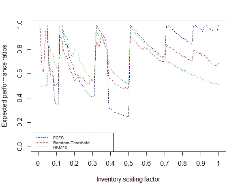
Figure 5: Computational performance using a real arrival sequence. The sequence is as shown in Equation (17).

When inventory level is either very small or very large, first-come-first-serve achieves near-optimal performance. This is not surprising, because FCFS always tries to accept an order if possible: when inventory is large then FCFS could almost accept everything except for the ones that arrive late. In our specific example shown in (17), the late items are fairly small – and this is why FCFS is near-optimal. On the other hand, when inventory is small then anything that FCFS successfully fits into the knapsack is already very large, relative to the small capacity. So FCFS has a near-optimal performance when inventory is very small. For scenarios where the starting inventory is of moderate size (i.e. for SKU’s that were neither overstocked nor understocked initially), our proposed algorithm has a relatively smaller variance.

5.1 Average and Worst-case Performance over all SKU’s

The earlier results shown for a specific SKU was used to illustrate the experimental setup. Now we show aggregate experimental results over all the SKU’s.

There are $974$ different SKU’s, carried in $21$ different warehouses over the country. For any fixed scaling factor, we first compute the average performance over different SKU’s.

We compute our Random-Threshold algorithm in the following manner. We take 21 evenly-spaced percentiles of the threshold distribution $F$, that is, we take the 21 thresholds defined by $F^{-1}(0),F^{-1}(0.05),...,F^{-1}(0.95),F^{-1}(1)$. These are 21 natural thresholds to be implemented over the 21 warehouses. Then we randomly permute them and assign them over the 21 warehouses, making accept/reject decisions at each warehouse based on the assigned threshold (scaled by the starting inventory). We then average the fulfillment ratios over the warehouses to determine the performance for a specific SKU. Finally we take an outer average over many independent random permutations of warehouses to define a final performance ratio for each SKU.

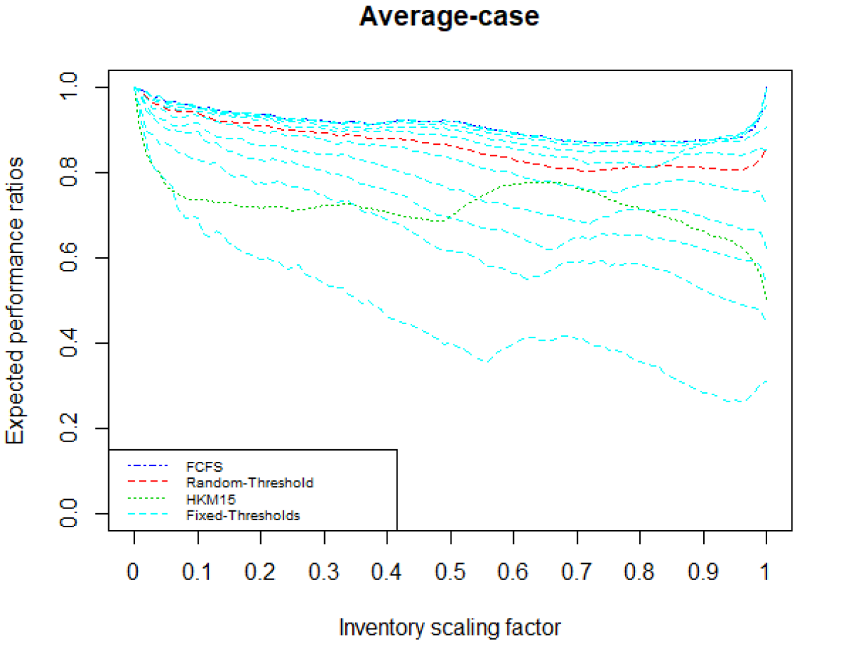
Figure 6: Computational of the average case performance using real arrival sequences over the country. The $10$ non-overlapping lines from top to bottom correspond to the ten fixed thresholds, $3\%,5\%,10\%,...,80\%$, respectively.

We compare our performance against the (deterministic) revenue from the greedy first-come-first-serve policy, named FCFS; the expected revenue from the algorithm suggested in Han et al. (2015), named HKM15; and the deterministic revenues of $10$ fixed-threshold algorithms, named Fixed-Thresholds. The fixed thresholds are re-scaled to be $3\%,5\%,10\%,15\%,20\%,30\%,40\%,50\%,60\%,80\%$ of the initial capacity. The results are shown in Figure 6, where we have divided all the numbers by its corresponding offline optimal integer packing. The performance of the Fixed-Thresholds algorithms have a decreasing performance ratio with respect to their thresholds. FCFS, if we interpret it as a threshold policy with threshold equal to zero, has the best performance. Interestingly, we integrate the CDF function and find the expected threshold suggested by our Random-Threshold policy to be roughly $28\%$ – and the performance of our Random-Threshold policy coincides to be between the $20\%$ and $30\%$ curves of the Fixed-Thresholds policies.

Again, we see that when inventory is either very small or very large, FCFS and the Fixed-Thresholds whose thresholds are small, they all achieve near-optimal performance. We find that the FCFS policy has the best average-case performance ratio. And the higher thresholds we increase for the Fixed-Thresholds, the worse performance it yields.

While this is discouraging, we believe that the way in which order sizes are censored in our data favors FCFS, since large orders cannot come at the end. Moreover, the gap between FCFS and our Random-Threshold algorithm is always smaller than $7\%$. Also, note that our Random-Threshold algorithm always outperforms HKM15. The gap between these two algorithms is between $5\%$–$27\%$.

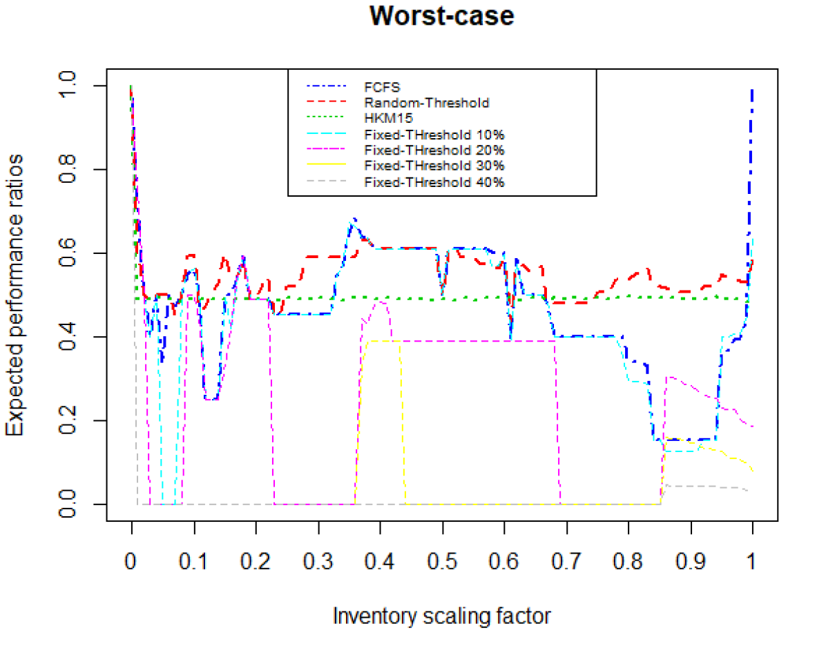
Figure 7: Computational of the worst case performance using real arrival sequences over the country. Some curves from Fixed-Thresholds are removed, for clarity.

Finally, to illustrate the benefit of our Random-Threshold algorithm, we also display the worst-case performance of each algorithm over the SKU’s, for each scaling factor. The computational results are shown in Figure 7.

Again, we see that when inventory is either very small or very large, FCFS, HKM15, our Random-Threshold, and the Fixed-Threshold algorithms whose thresholds are small all achieve near-optimal performance. However, our Random-Threshold algorithm has the best worst-case performance for a large fraction of scaling factors. This shows that setting different thresholds at different warehouses, according to the distributions we derived, indeed provides the best baseline guarantee on the fulfillment of any SKU.

We see that as we increase the thresholds, the Fixed-Threshold policies tend to have worse performance. Note that the performance of FCFS or any Fixed-Threshold policy does not have any guarantee – FCFS and the Fixed-Threshold policies whose thresholds are less or equal to $5\%$ can have a performance as bad as 15%; and the Fixed-Threshold policies whose thresholds are at least $10\%$ can have a worst-case performance guarantee of 0. By contrast, the worst-case performance of our algorithm over all of the scaling factors is $44\%$ (close to the theoretical guarantee of 43%). Meanwhile, the performance for HKM15 always equals its theoretical guarantee of 50%.

6 Conclusion

In this paper, we study an online knapsack problem and its competitive analysis. We focus on a particular class of random threshold algorithms, that initially draw a random threshold and never change the threshold throughout the entire horizon. This class of algorithms benefit us from simplicity, applicability, and incentive-compatibility, which are important in real-world applications.

We start from the single knapsack problem, and study its generalization to the multiple knapsack problems. We provide constant factor competitive results that are tight on a single knapsack, relative to two different offline optimal packing optimum. Numerical experiments suggest that the performance is better than merely our theoretical guarantees.

Finally, we conclude our paper by pointing out a few possible extensions to this paper. Firstly, we could extend our model to consider multiple consumptions over different knapsacks. Suppose we are managing a manufacturing plant that requires different resources to make products, instead of a warehouse managing a single stock. One arriving item could potentially require more than one single resource to be produced. For each unit of resource consumed, there is an associated revenue / cost. Our goal is to maximize the total revenue / minimize the total cost throughout the horizon.

We could also extend our model to reusable products. Suppose there is a fixed total amount of cloud computing resources whose capacity is 1, and an unknown sequence of tasks with sizes at most 1. The tasks arrive one-by-one, and each task must be irrevocably either assigned to some amount of computing resources, or immediately discarded upon arrival. A task can be accepted only if its requested resources do not exceed the remaining resource capacity. Associated with each accepted task, there is a usage time after which the computing resources can be returned. These resources immediately become available after the usage time. If one unit of resource is occupied for one period of time, a constant amount of revenue is generated. Our goal is to maximize the total revenue generated throughout the horizon.

E-Companion

7 Proof of Theorem 3.9

Proof 7.1

Proof of Theorem 3.9. We are going to show that, for any instance of arrival sequence $S$, we have $\frac{\mathsf{ALG}_{\mathsf{N\ref{defn:0.432alg}}}(S)}{\mathsf{OPT}(S)}\geq c_{\textit{N\ref{defn:0.432alg}}}$. We lower bound $\mathsf{ALG}_{\mathsf{N\ref{defn:0.432alg}}}(S)$ and upper bound $\mathsf{OPT}(S)$ at the same time.

First of all, $\mathsf{Greedy}$ always accepts something. Denote the set of items accepted by $\mathsf{Greedy}$ as $G$. Denote $\mathsf{size}(G)=g$. If $G=[T]$ then $\mathsf{Greedy}$ is optimal. In this case

$$\frac{\mathsf{ALG}_{\mathsf{N\ref{defn:0.432alg}}}}{\mathsf{OPT}}\geq\Pr(\tau=0)\cdot 1+\Pr(\tau>0)\cdot 0\geq F_{\textit{N\ref{defn:0.432alg}}}(0)=1-c_{\textit{N\ref{defn:0.432alg}}}\geq c_{\textit{N\ref{defn:0.432alg}}}.$$

If $G\subsetneqq[T]$, let $M=[T]\backslash G$ denote the set of items blocked by $\mathsf{Greedy}$. Since $\mathsf{Greedy}$ always accepts an item as long as it can fill in, any item blocked by $\mathsf{Greedy}$ must exceed the remaining space of the knapsack, at the moment it is blocked. We also know that $G\cup M=[T]$, $G\cap M=\phi$.

Let $m$ be the smallest size in $M$, i.e. $m=\min_{t\in M}s_{t}$. Define index $t_{m}$ for the smallest item, or the first smallest item, if there are multiple smallest items.

$$t_{m}=\min\left\{t\in[T]\left|s_{t}=m\right.\right\}.$$ (18)

Denote $G^{\prime}$ as the set of items accepted by $\mathsf{Greedy}$, at the moment $s_{t_{m}}$ is blocked. Let $g^{\prime}=\mathsf{size}(G^{\prime})$. See Figure 2. A straightforward, but useful information about $m$ is:

$$g^{\prime}+m>1,$$ (19)

because $m$ is blocked by $\mathsf{Greedy}$. We wish to understand when we can admit an item of size at least $m$, by selecting a proper threshold $\tau$.

We distinguish two cases: $m>1/2$ and $m\leq 1/2$.

Case 1: $m>1/2$.
Let $S^{\mathsf{THR}}(\tau)$ be the set of items that have sizes at least $\tau$, i.e. $S^{\mathsf{THR}}(\tau)=\left\{t\in S\left|s_{t}\geq\tau\right.\right\}$. Now define

$$\begin{split}q=\max&\quad\tau\\ s.t.&\quad m+\mathsf{size}(S^{\mathsf{THR}}(\tau)\cap G^{\prime})>1\end{split}$$ (20)

This means that if we adopt a $\mathsf{THR}(q)$ policy, then the size $m$ item must be blocked (possibly it will also be rejected, due to $q>m$).

Now consider the items in $S^{\mathsf{THR}}(q)\cap G^{\prime}$. See Figure 3. These items have sizes at least $q$. We count how many size $q$ items are there, and let $n$ be the number of size $q$ items. Denote the total size of the remaining items be $x$. We know that

$$\mathsf{size}(S^{\mathsf{THR}}(q)\cap G^{\prime})=nq+x.$$ (21)

We make the following observations:

1. There must exist some item from $G^{\prime}$ that is of size $q$, i.e.

   $$\exists t_{q}\in G^{\prime}\subseteq[T],s.t.\ s_{t_{q}}=q.$$ (22)

   This is because otherwise we can select the smallest item size in $G^{\prime}$ that is also larger than $q$. This item size satisfies (20), and violates the maximum property of $q$.

2. Size $m$ items can not fit in together with items $S^{\mathsf{THR}}(q)\cap G^{\prime}$, i.e.

   $$nq+x+m>1$$ (23)

   This is because $\mathsf{size}(S^{\mathsf{THR}}(q)\cap G^{\prime})=nq+x$. This is implied by (20).

3. A size $m$ item can fit in together with items $S^{\mathsf{THR}}(\tau)\cap G^{\prime},\forall\tau>q$, i.e.

   $$x+m\leq 1$$ (24)

   This is because otherwise we could further increase $q$ to $\hat{q}$ so that $\mathsf{size}(S^{\mathsf{THR}}(\hat{q})\cap G^{\prime})+m>1$, which violates the maximum property of $q$.

We further distinguish two cases: $q>m$, and $q\leq m$.

Case 1.1: $q>m$.
In this case, if we adopt $\mathsf{Greedy}$ then we can get as much as $g$. This is because $g$ is defined this way.

If we adopt $\mathsf{THR}(\tau),\forall\tau\in(0,q]$ then we can get no less than $q$. This is because due to (22) there must exist some item $t_{q}\in G^{\prime}$ of size $q$. We either accept it, in which case we immediately earn $q$, or we have blocked it because we admitted some item $z\in[T]$ from $M$ and consumed too much space. But $\mathsf{Greedy}$ blocks item $z$ earlier than it accepts item $t_{q}$, which means that $s_{z}\geq s_{t_{q}}=q$. So in either case we earn $q$.

We have the following:

$$\mathsf{ALG}_{\mathsf{N\ref{defn:0.432alg}}} \geq\Pr(\tau=0)\cdot g+\Pr(0<\tau\leq q)\cdot q$$

$$=F_{\textit{N\ref{defn:0.432alg}}}(0)\cdot g+(F_{\textit{N\ref{defn:0.432alg}}}(q)-F_{\textit{N\ref{defn:0.432alg}}}(0))\cdot q$$

$$\geq F_{\textit{N\ref{defn:0.432alg}}}(0)\cdot(1-2q)+F_{\textit{N\ref{defn:0.432alg}}}(q)\cdot q$$

$$=(1-c_{\textit{N\ref{defn:0.432alg}}})\cdot(1-2q)+\left[2(1-c_{\textit{N\ref{defn:0.432alg}}})-\frac{1-2c_{\textit{N\ref{defn:0.432alg}}}}{q}\right]\cdot q$$

$$=c_{\textit{N\ref{defn:0.432alg}}}$$

where the second inequality is because $g\geq g^{\prime}>1-m$ (due to (19)) and $1-m>1-q$ (Case 1.1: $q>m$); second equality is because $q>m\geq 1/2>q_{\textit{N\ref{defn:0.432alg}}}$, so we plug in $F_{\textit{N\ref{defn:0.432alg}}}(\cdot)$ as defined in (14).

Since $\mathsf{OPT}\leq 1$, we have $\frac{\mathsf{ALG}}{\mathsf{OPT}}\geq c_{\textit{N\ref{defn:0.432alg}}}$.

Case 1.2: $q\leq m$.
First we wish to upper bound $\mathsf{OPT}$. $\mathsf{OPT}$ selects some items from $[T]=G\cup M$, where $G\cap M=\phi$. Notice that $m>1/2$ so there is at most $1$ item from $M$ that $\mathsf{OPT}$ can select. If $\mathsf{OPT}$ selects no item from $M$, then $\mathsf{OPT}\leq g$. With probability $F_{\textit{N\ref{defn:0.432alg}}}(0)$, $\mathsf{ALG}_{\mathsf{N\ref{defn:0.432alg}}}$ adopts $\mathsf{Greedy}$ and earns $g$. So we have

$$\frac{\mathsf{ALG}_{\mathsf{N\ref{defn:0.432alg}}}}{\mathsf{OPT}}\geq\Pr(\tau=0)\cdot 1+\Pr(\tau>0)\cdot 0\geq F_{\textit{N\ref{defn:0.432alg}}}(0)=1-c_{\textit{N\ref{defn:0.432alg}}}\geq c_{\textit{N\ref{defn:0.432alg}}}.$$

If $\mathsf{OPT}$ selects one item from $M$, let $t_{m^{\prime}}\in[T]$ be this item. So $s_{t_{m^{\prime}}}=m^{\prime}\geq m$. See Figure 8.

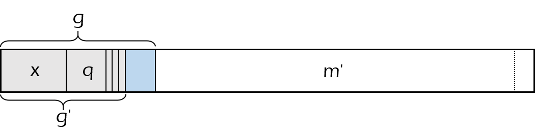
Figure 8: Illustration of the items accepted by $\mathsf{OPT}$

We can partition all the items in $S$ into three sets:

$$M; S^{\mathsf{THR}}(q)\cap G^{\prime}; G\backslash(S^{\mathsf{THR}}(q)\cap G^{\prime})$$

Let $\tilde{g}=\mathsf{size}(G\backslash(S^{\mathsf{THR}}(q)\cap G^{\prime}))$. Since $S^{\mathsf{THR}}(q)\cap G^{\prime}$ and $G\backslash(S^{\mathsf{THR}}(q)\cap G^{\prime})$ form a partition of $G$, we have $g=(nq+x)+\tilde{g}$. From (23) we know that $m^{\prime}+\mathsf{size}(S^{\mathsf{THR}}(q)\cap G^{\prime})\geq m+\mathsf{size}(S^{\mathsf{THR}}(q)\cap G^{\prime})>1$. This means that even $\mathsf{OPT}$ cannot pack $s_{t_{m^{\prime}}}$ and $S^{\mathsf{THR}}(q)\cap G^{\prime}$ together. $\mathsf{OPT}$ must block at least one item from $\{t_{m^{\prime}}\}\cup(S^{\mathsf{THR}}(q)\cap G^{\prime})$ – and the smallest item from this union is of size $q$ (because $q\leq m\leq m^{\prime}$). So we upper bound $\mathsf{OPT}$ by:

$$\begin{split}\mathsf{OPT}\leq&\min\left\{1,\left[m^{\prime}+\mathsf{size}(S^{\mathsf{THR}}(q)\cap G^{\prime})\right]-q+\mathsf{size}(G\backslash(S^{\mathsf{THR}}(q)\cap G^{\prime}))\right\}\\ =&\min\left\{1,m^{\prime}+(nq+x)-q+\tilde{g}\right\}\end{split}$$ (25)

Then we analyze $\mathsf{ALG}_{\mathsf{N\ref{defn:0.432alg}}}$. If we adopt $\mathsf{Greedy}$ then we can get as much as $g$. This is because $g$ is defined this way.

If we adopt $\mathsf{THR}(\tau),\forall\tau\in(0,q]$ then we get no less than $nq+x$. This is because due to (21) there must exist some items in $S^{\mathsf{THR}}(q)\cap G^{\prime}$, which are of size $nq+x$. For any subset of items $S_{0}\subseteq(S^{\mathsf{THR}}(q)\cap G^{\prime})$, we either accept it, in which case we immediately earn $\mathsf{size}(S_{0})$, or we have blocked it because we admitted some item $z\in[T]$ from $M$ and consumed too much space. But $\mathsf{Greedy}$ blocks item $z$ earlier than it accepts $S_{0}$, which means that $s_{z}\geq\mathsf{size}(S_{0})$. So in either case we earn $\mathsf{size}(S_{0})$. Since $S_{0}$ is chosen arbitrarily, we will always get at least $nq+x$.

If we adopt $\mathsf{THR}(\tau),\forall\tau\in(q,m]$ then we get no less than $m$. This is because due to (24), any item in $S^{\mathsf{THR}}(\tau)\cap G^{\prime}$ will not block item $t_{m}$ (from expression (18)); and $\tau\leq m$ so we will not reject item $t_{m}$. We either accept item $t_{m}$, in which case we immediately earn $m$, or we have blocked it because we admitted some item $z\in[T]$ from M and consumed too much space. But $m$ is smallest item size in $M$, which means that $s_{z}\geq m$. So in either case we earn $m$.

If we adopt $\mathsf{THR}(\tau),\forall\tau\in(m,m^{\prime}]$ then we get no less than $\tau$. This is because $s_{t_{m^{\prime}}}$ does exist, and $\mathsf{THR}(\tau)$ must accept at least one item. The least that $\mathsf{THR}(\tau)$ can get is $\tau$.

We have the following:

$$\mathsf{ALG}_{\mathsf{N\ref{defn:0.432alg}}} \geq\Pr(\tau=0)\cdot g+\Pr(0<\tau\leq q)\cdot(nq+x)+\Pr(q<\tau\leq m)\cdot m+\int_{m}^{m^{\prime}}\tau\ \mathrm{d}F_{\textit{N\ref{defn:0.432alg}}}(\tau)$$

$$=F_{\textit{N\ref{defn:0.432alg}}}(0)\cdot(nq+x+\tilde{g})+(F_{\textit{N\ref{defn:0.432alg}}}(q)-F_{\textit{N\ref{defn:0.432alg}}}(0))\cdot(nq+x)+(F_{\textit{N\ref{defn:0.432alg}}}(m)-F_{\textit{N\ref{defn:0.432alg}}}(q))\cdot m+\int_{m}^{m^{\prime}}\tau\ \mathrm{d}F_{\textit{N\ref{defn:0.432alg}}}(\tau)$$

$$=F_{\textit{N\ref{defn:0.432alg}}}(0)\cdot\tilde{g}+F_{\textit{N\ref{defn:0.432alg}}}(q)\cdot(nq+x-m)+F_{\textit{N\ref{defn:0.432alg}}}(m^{\prime})\cdot m^{\prime}-\int_{m}^{m^{\prime}}F_{\textit{N\ref{defn:0.432alg}}}(\tau)\ \mathrm{d}\tau$$

$$\geq F_{\textit{N\ref{defn:0.432alg}}}(0)\cdot\tilde{g}+F_{\textit{N\ref{defn:0.432alg}}}(q)\cdot(2(nq+x)-1)+F_{\textit{N\ref{defn:0.432alg}}}(m^{\prime})\cdot m^{\prime}-\int_{1-(nq+x)}^{m^{\prime}}F_{\textit{N\ref{defn:0.432alg}}}(\tau)\ \mathrm{d}\tau$$

where the second equality is due to integration by part (our definition of $F_{\textit{N\ref{defn:0.432alg}}}(\cdot)$ in (14) is a continuous function); the last inequality is because $\frac{\partial\mathsf{ALG}_{\mathsf{N\ref{defn:0.432alg}}}}{\partial m}=F_{\textit{N\ref{defn:0.432alg}}}(m)-F_{\textit{N\ref{defn:0.432alg}}}(q)\geq 0$, (because $q\leq m$, and $F_{\textit{N\ref{defn:0.432alg}}}(\cdot)$ is a increasing function), so that $\mathsf{ALG}_{\mathsf{N\ref{defn:0.432alg}}}$ is increasing in $m$. Hence, $\mathsf{ALG}_{\mathsf{N\ref{defn:0.432alg}}}$ achieves its minimum when $m$ is the smallest, and $m>1-(nq+x)$ from (23).

Observe that

$$\mathsf{ALG}_{\mathsf{N\ref{defn:0.432alg}}}-c_{\textit{N\ref{defn:0.432alg}}}\mathsf{OPT}\geq F_{\textit{N\ref{defn:0.432alg}}}(0)\cdot\tilde{g}+F_{\textit{N\ref{defn:0.432alg}}}(q)\cdot(2(nq+x)-1)+F_{\textit{N\ref{defn:0.432alg}}}(m^{\prime})\cdot m^{\prime}-\int_{1-(nq+x)}^{m^{\prime}}F_{\textit{N\ref{defn:0.432alg}}}(\tau)\ \mathrm{d}\tau$$

$$\quad-c_{\textit{N\ref{defn:0.432alg}}}\cdot\min\left\{1,m^{\prime}+(nq+x)-q+\tilde{g}\right\}$$

If we focus on the dependence of $\tilde{g}$, we find that

$$\frac{\partial\left(\mathsf{ALG}_{\mathsf{N\ref{defn:0.432alg}}}-c_{\textit{N\ref{defn:0.432alg}}}\mathsf{OPT}\right)}{\partial\tilde{g}}\geq F_{\textit{N\ref{defn:0.432alg}}}(0)-c_{\textit{N\ref{defn:0.432alg}}}=1-2c_{\textit{N\ref{defn:0.432alg}}}\geq 0,$$

where the first inequality is because the subgradient of the subtracted term is either $0$ or $c_{\textit{N\ref{defn:0.432alg}}}$. Since $\mathsf{ALG}_{\mathsf{N\ref{defn:0.432alg}}}-c_{\textit{N\ref{defn:0.432alg}}}\mathsf{OPT}$ is a increasing function of $\tilde{g}$, it achieves its minimum when $\tilde{g}=0$.

We have further

$$\mathsf{ALG}_{\mathsf{N\ref{defn:0.432alg}}}-c_{\textit{N\ref{defn:0.432alg}}}\mathsf{OPT}\geq F_{\textit{N\ref{defn:0.432alg}}}(q)\cdot(2(nq+x)-1)+F_{\textit{N\ref{defn:0.432alg}}}(m^{\prime})\cdot m^{\prime}-\int_{1-(nq+x)}^{m^{\prime}}F_{\textit{N\ref{defn:0.432alg}}}(\tau)\ \mathrm{d}\tau-c_{\textit{N\ref{defn:0.432alg}}}\cdot\min\left\{1,m^{\prime}+(nq+x)-q\right\}$$

Now let $y=(n-1)q+x$, and we plug in $F_{\textit{N\ref{defn:0.432alg}}}(\cdot)$ as we defined in (23).

Case 1.2.1: When $q\leq q_{\textit{N\ref{defn:0.432alg}}}$, we have:

$$\mathsf{ALG}_{\mathsf{N\ref{defn:0.432alg}}}-c_{\textit{N\ref{defn:0.432alg}}}\mathsf{OPT}$$

$$\geq F_{\textit{N\ref{defn:0.432alg}}}(q)\cdot(2(q+y)-1)+F_{\textit{N\ref{defn:0.432alg}}}(m^{\prime})\cdot m^{\prime}-\int_{1-(q+y)}^{m^{\prime}}F_{\textit{N\ref{defn:0.432alg}}}(\tau)\ \mathrm{d}\tau-c_{\textit{N\ref{defn:0.432alg}}}\cdot\min\left\{1,m^{\prime}+y\right\}$$

$$= (1-c_{\textit{N\ref{defn:0.432alg}}})(2(q+y)-1)+\frac{(2q-1+2y)(1-2c_{\textit{N\ref{defn:0.432alg}}})\ln{(1-q)}}{2q-1}+2(1-c_{\textit{N\ref{defn:0.432alg}}})m^{\prime}-(1-2c_{\textit{N\ref{defn:0.432alg}}})$$

$$-2(1-c_{\textit{N\ref{defn:0.432alg}}})m^{\prime}+2(1-c_{\textit{N\ref{defn:0.432alg}}})[1-(q+y)]+(1-2c_{\textit{N\ref{defn:0.432alg}}})\left[\ln{m^{\prime}}-\ln{(1-(q+y))}\right]-c_{\textit{N\ref{defn:0.432alg}}}\cdot\min\left\{1,m^{\prime}+y\right\}$$

$$= c_{\textit{N\ref{defn:0.432alg}}}+\frac{(2q-1+2y)(1-2c_{\textit{N\ref{defn:0.432alg}}})\ln{(1-q)}}{2q-1}+(1-2c_{\textit{N\ref{defn:0.432alg}}})\left[\ln{m^{\prime}}-\ln{(1-(q+y))}\right]-c_{\textit{N\ref{defn:0.432alg}}}\cdot\min\left\{1,m^{\prime}+y\right\}$$

If we focus on the dependence of $m^{\prime}$, we will see that $\mathsf{ALG}_{\mathsf{N\ref{defn:0.432alg}}}-c_{\textit{N\ref{defn:0.432alg}}}\mathsf{OPT}$ has only one local minimum: when $m^{\prime}<1-y$ we have

$$\frac{\partial\left(\mathsf{ALG}_{\mathsf{N\ref{defn:0.432alg}}}-c_{\textit{N\ref{defn:0.432alg}}}\mathsf{OPT}\right)}{\partial m^{\prime}}=\frac{1-2c_{\textit{N\ref{defn:0.432alg}}}}{m^{\prime}}-c_{\textit{N\ref{defn:0.432alg}}}\leq\frac{1-2c_{\textit{N\ref{defn:0.432alg}}}}{1/2}-c_{\textit{N\ref{defn:0.432alg}}}=2-5c_{\textit{N\ref{defn:0.432alg}}}<0,$$

because $m^{\prime}\geq m\geq 1/2$. So $\mathsf{ALG}_{\mathsf{N\ref{defn:0.432alg}}}-c_{\textit{N\ref{defn:0.432alg}}}\mathsf{OPT}$ is decreasing on $m^{\prime}$ when $m^{\prime}<1-y$. When $m^{\prime}>1-y$ we have

$$\frac{\partial\left(\mathsf{ALG}_{\mathsf{N\ref{defn:0.432alg}}}-c_{\textit{N\ref{defn:0.432alg}}}\mathsf{OPT}\right)}{\partial m^{\prime}}=\frac{1-2c_{\textit{N\ref{defn:0.432alg}}}}{m^{\prime}}>0,$$

so $\mathsf{ALG}_{\mathsf{N\ref{defn:0.432alg}}}-c_{\textit{N\ref{defn:0.432alg}}}\mathsf{OPT}$ is increasing on $m^{\prime}$. Hence, $\mathsf{ALG}_{\mathsf{N\ref{defn:0.432alg}}}-c_{\textit{N\ref{defn:0.432alg}}}\mathsf{OPT}$ achieves its minimum when $m^{\prime}=1-y$.

Plugging into $m^{\prime}=1-y$, we have further

$$\mathsf{ALG}_{\mathsf{N\ref{defn:0.432alg}}}-c_{\textit{N\ref{defn:0.432alg}}}\mathsf{OPT}\geq \frac{(2q-1+2y)(1-2c_{\textit{N\ref{defn:0.432alg}}})\ln{(1-q)}}{2q-1}+(1-2c_{\textit{N\ref{defn:0.432alg}}})\left[\ln{(1-y)}-\ln{(1-(q+y))}\right]$$

If we focus on the dependence of $y$, we find that

$$\frac{\partial\left(\mathsf{ALG}_{\mathsf{N\ref{defn:0.432alg}}}-c_{\textit{N\ref{defn:0.432alg}}}\mathsf{OPT}\right)}{\partial y}=(1-2c_{\textit{N\ref{defn:0.432alg}}})\left[2\frac{\ln{(1-q)}}{2q-1}-\frac{1}{1-y}+\frac{1}{1-y-q}\right]>0,$$

because $ln{(1-q)}<0,2q-1<2q_{\textit{N\ref{defn:0.432alg}}}-1<0,\frac{1}{1-y-q}-\frac{1}{1-y}\geq 0$. Since $\mathsf{ALG}_{\mathsf{N\ref{defn:0.432alg}}}-c_{\textit{N\ref{defn:0.432alg}}}\mathsf{OPT}$ is increasing on $y$, it achieves its minimum when $y=0$.

Finally, plugging into $y=0$, we have

$$\mathsf{ALG}_{\mathsf{N\ref{defn:0.432alg}}}-c_{\textit{N\ref{defn:0.432alg}}}\mathsf{OPT}\geq \frac{(2q-1)(1-2c_{\textit{N\ref{defn:0.432alg}}})\ln{(1-q)}}{2q-1}-(1-2c_{\textit{N\ref{defn:0.432alg}}})\ln{(1-q)}=0$$

Case 1.2.2: When $q>q_{\textit{N\ref{defn:0.432alg}}}$, we have:

$$\mathsf{ALG}_{\mathsf{N\ref{defn:0.432alg}}}-c_{\textit{N\ref{defn:0.432alg}}}\mathsf{OPT}$$

$$\geq F_{\textit{N\ref{defn:0.432alg}}}(q)\cdot(2(q+y)-1)+F_{\textit{N\ref{defn:0.432alg}}}(m^{\prime})\cdot m^{\prime}-\int_{1-(q+y)}^{m^{\prime}}F_{\textit{N\ref{defn:0.432alg}}}(\tau)\ \mathrm{d}\tau-c_{\textit{N\ref{defn:0.432alg}}}\cdot\min\left\{1,m^{\prime}+y\right\}$$

$$= 2(1-c_{\textit{N\ref{defn:0.432alg}}})(2(q+y)-1)-\frac{(1-2c_{\textit{N\ref{defn:0.432alg}}})(2(q+y)-1)}{q}+2(1-c_{\textit{N\ref{defn:0.432alg}}})m^{\prime}-(1-2c_{\textit{N\ref{defn:0.432alg}}})$$

$$-2(1-c_{\textit{N\ref{defn:0.432alg}}})m^{\prime}+2(1-c_{\textit{N\ref{defn:0.432alg}}})[1-(q+y)]+(1-2c_{\textit{N\ref{defn:0.432alg}}})\left[\ln{m^{\prime}}-\ln{(1-(q+y))}\right]-c_{\textit{N\ref{defn:0.432alg}}}\cdot\min\left\{1,m^{\prime}+y\right\}$$

$$= 2(1-c_{\textit{N\ref{defn:0.432alg}}})(y+q)-(1-2c_{\textit{N\ref{defn:0.432alg}}})-\frac{(1-2c_{\textit{N\ref{defn:0.432alg}}})(2(q+y)-1)}{q}$$

$$+(1-2c_{\textit{N\ref{defn:0.432alg}}})\left[\ln{m^{\prime}}-\ln{(1-(q+y))}\right]-c_{\textit{N\ref{defn:0.432alg}}}\cdot\min\left\{1,m^{\prime}+y\right\}$$

Again, if we focus on the dependence of $m^{\prime}$, we will see that $\mathsf{ALG}_{\mathsf{N\ref{defn:0.432alg}}}-c_{\textit{N\ref{defn:0.432alg}}}\mathsf{OPT}$ has only one local minimum when $m^{\prime}=1-y$.

Plugging into $m^{\prime}=1-y$, we have further

$$\mathsf{ALG}_{\mathsf{N\ref{defn:0.432alg}}}-c_{\textit{N\ref{defn:0.432alg}}}\mathsf{OPT}\geq (1-c_{\textit{N\ref{defn:0.432alg}}})(2(y+q)-1)-\frac{(1-2c_{\textit{N\ref{defn:0.432alg}}})(2(q+y)-1)}{q}+(1-2c_{\textit{N\ref{defn:0.432alg}}})\left[\ln{(1-y)}-\ln{(1-(q+y))}\right]$$

Again, if we focus on the dependence of $y$, we find that

$$\frac{\partial\left(\mathsf{ALG}_{\mathsf{N\ref{defn:0.432alg}}}-c_{\textit{N\ref{defn:0.432alg}}}\mathsf{OPT}\right)}{\partial y}=2(1-c_{\textit{N\ref{defn:0.432alg}}}-\frac{1-2c_{\textit{N\ref{defn:0.432alg}}}}{q})+(1-2c_{\textit{N\ref{defn:0.432alg}}})\left[-\frac{1}{1-y}+\frac{1}{1-y-q}\right]>0,$$

because $1-c_{\textit{N\ref{defn:0.432alg}}}-\frac{1-2c_{\textit{N\ref{defn:0.432alg}}}}{q}\geq 1-c_{\textit{N\ref{defn:0.432alg}}}-\frac{1-2c_{\textit{N\ref{defn:0.432alg}}}}{q_{\textit{N\ref{defn:0.432alg}}}}\approx 0.142>0,\frac{1}{1-y-q}-\frac{1}{1-y}\geq 0$. Since $\mathsf{ALG}_{\mathsf{N\ref{defn:0.432alg}}}-c_{\textit{N\ref{defn:0.432alg}}}\mathsf{OPT}$ is increasing on $y$, it achieves its minimum when $y=0$.

Finally, plugging into $y=0$, we have

$$\mathsf{ALG}_{\mathsf{N\ref{defn:0.432alg}}}-c_{\textit{N\ref{defn:0.432alg}}}\mathsf{OPT}\geq (1-c_{\textit{N\ref{defn:0.432alg}}})(2q-1)-\frac{(1-2c_{\textit{N\ref{defn:0.432alg}}})(2q-1)}{q}-(1-2c_{\textit{N\ref{defn:0.432alg}}})\ln{(1-q)}$$

$$= (2q-1)\left[(1-c_{\textit{N\ref{defn:0.432alg}}})-\frac{(1-2c_{\textit{N\ref{defn:0.432alg}}})}{q}\right]-(1-2c_{\textit{N\ref{defn:0.432alg}}})\ln{(1-q)}$$

$$\geq (2q-1)\left[-\frac{(1-2c_{\textit{N\ref{defn:0.432alg}}})\ln{(1-q)}}{1-2q}\right]-(1-2c_{\textit{N\ref{defn:0.432alg}}})\ln{(1-q)}$$

$$= 0$$

where the second inequality is because $H(c_{\textit{N\ref{defn:0.432alg}}},q)=\frac{1-2c_{\textit{N\ref{defn:0.432alg}}}}{q}-\frac{(1-2c_{\textit{N\ref{defn:0.432alg}}})\ln{(1-q)}}{1-2q}-(1-c_{\textit{N\ref{defn:0.432alg}}})\geq 0,\forall q\in(0,1/2)$ from (13), and when $q\in[1/2,1]$, the second line expression is an increasing function of $q$ (because $2q-1;(1-c_{\textit{N\ref{defn:0.432alg}}})-\frac{(1-2c_{\textit{N\ref{defn:0.432alg}}})}{q};$ and $-(1-2c_{\textit{N\ref{defn:0.432alg}}})\ln{(1-q)}$ are all increasing in $q$), thus plugging in $q=1/2$ we have $\mathsf{ALG}_{\mathsf{N\ref{defn:0.432alg}}}-c_{\textit{N\ref{defn:0.432alg}}}\mathsf{OPT}\geq-(1-2c_{\textit{N\ref{defn:0.432alg}}})\ln{(1-q)}>0$.

In all, $\mathsf{ALG}_{\mathsf{N\ref{defn:0.432alg}}}\geq c_{\textit{N\ref{defn:0.432alg}}}\mathsf{OPT}$.

Case 2: $m\leq 1/2$.
In this case, we only hope to get $m$, and a crude analysis is enough. See Figure 4.

If we adopt $\mathsf{Greedy}$ then we can get as much as $g$. This is because $g$ is defined this way.

If we adopt $\mathsf{THR}(\tau),\forall\tau\in(0,m]$ then we either get $m$, or $m$ is blocked, in which case we must have already earned at least $1-m$ to block $m$.

We have the following:

$$\mathsf{ALG} \geq\Pr(\tau=0)\cdot g+\Pr(0<\tau\leq m)\cdot\min\{m,1-m\}$$

$$\geq\Pr(\tau=0)\cdot g+\Pr(0<\tau\leq m)\cdot m$$

$$=F_{\textit{N\ref{defn:0.432alg}}}(0)\cdot g+(F_{\textit{N\ref{defn:0.432alg}}}(m)-F_{\textit{N\ref{defn:0.432alg}}}(0))\cdot m$$

$$\geq F_{\textit{N\ref{defn:0.432alg}}}(0)\cdot(1-m)+(F_{\textit{N\ref{defn:0.432alg}}}(m)-F_{\textit{N\ref{defn:0.432alg}}}(0))\cdot m$$

$$=F_{\textit{N\ref{defn:0.432alg}}}(0)\cdot(1-2m)+F_{\textit{N\ref{defn:0.432alg}}}(m)\cdot m$$

$$=(1-c_{\textit{N\ref{defn:0.432alg}}})(1-2m)+\left[2(1-c_{\textit{N\ref{defn:0.432alg}}})-\frac{1-2c_{\textit{N\ref{defn:0.432alg}}}}{m}\right]\cdot m$$

$$=c_{\textit{N\ref{defn:0.432alg}}}$$

where the second inequality is because $m\leq 1/2$; the last inequality is because $g\geq g^{\prime}>1-m$ (due to (19)); the third equality is because we plug in $F_{\textit{N\ref{defn:0.432alg}}}(\cdot)$ as defined in (14).

Since $\mathsf{OPT}\leq 1$, we have $\frac{\mathsf{ALG}}{\mathsf{OPT}}\geq c_{\textit{N\ref{defn:0.432alg}}}$.

In all, we have enumerated all the possible cases, to find $\dfrac{\mathsf{ALG}}{\mathsf{OPT}}\geq c_{\textit{N\ref{defn:0.432alg}}}$ always holds.

References

- Assadi et al. (2015) Assadi S, Hsu J, Jabbari S (2015) Online assignment of heterogeneous tasks in crowdsourcing markets. Third AAAI Conference on Human Computation and Crowdsourcing.
- Bansak et al. (2018) Bansak K, Ferwerda J, Hainmueller J, Dillon A, Hangartner D, Lawrence D, Weinstein J (2018) Improving refugee integration through data-driven algorithmic assignment. Science 359(6373):325–329.
- Cygan et al. (2016) Cygan M, Jeż Ł, Sgall J (2016) Online knapsack revisited. Theory of Computing Systems 58(1):153–190.
- Dean et al. (2008) Dean BC, Goemans MX, Vondrák J (2008) Approximating the stochastic knapsack problem: The benefit of adaptivity. Mathematics of Operations Research 33(4):945–964.
- Dwork et al. (2012) Dwork C, Hardt M, Pitassi T, Reingold O, Zemel R (2012) Fairness through awareness. Proceedings of the 3rd innovations in theoretical computer science conference, 214–226 (ACM).
- Gupta and Kamble (2019) Gupta S, Kamble V (2019) Individual fairness in hindsight. Proceedings of the 2019 ACM Conference on Economics and Computation, 805–806 (ACM).
- Han et al. (2015) Han X, Kawase Y, Makino K (2015) Randomized algorithms for online knapsack problems. Theoretical Computer Science 562:395–405.
- Ho and Vaughan (2012) Ho CJ, Vaughan JW (2012) Online task assignment in crowdsourcing markets. Twenty-Sixth AAAI Conference on Artificial Intelligence.
- Hwang et al. (2018) Hwang D, Jaillet P, Manshadi V (2018) Online resource allocation under partially predictable demand. arXiv preprint arXiv:1810.00447 .
- Karp et al. (1990) Karp RM, Vazirani UV, Vazirani VV (1990) An optimal algorithm for on-line bipartite matching. Proceedings of the twenty-second annual ACM symposium on Theory of computing, 352–358 (ACM).
- Kleywegt and Papastavrou (1998) Kleywegt AJ, Papastavrou JD (1998) The dynamic and stochastic knapsack problem. Operations research 46(1):17–35.
- Liu and Van Ryzin (2008) Liu Q, Van Ryzin G (2008) On the choice-based linear programming model for network revenue management. Manufacturing & Service Operations Management 10(2):288–310.
- Marchetti-Spaccamela and Vercellis (1995) Marchetti-Spaccamela A, Vercellis C (1995) Stochastic on-line knapsack problems. Mathematical Programming 68(1-3):73–104.
- Mehta et al. (2005) Mehta A, Saberi A, Vazirani U, Vazirani V (2005) Adwords and generalized on-line matching. 46th Annual IEEE Symposium on Foundations of Computer Science (FOCS’05), 264–273 (IEEE).
- Mehta et al. (2013) Mehta A, et al. (2013) Online matching and ad allocation. Foundations and Trends® in Theoretical Computer Science 8(4):265–368.
- Modaresi et al. (2019) Modaresi S, Saure D, Vielma JP (2019) Learning in combinatorial optimization: What and how to explore. Available at SSRN 3041893 .
- Papastavrou et al. (1996) Papastavrou JD, Rajagopalan S, Kleywegt AJ (1996) The dynamic and stochastic knapsack problem with deadlines. Management Science 42(12):1706–1718.
- Stein et al. (2018) Stein C, Truong VA, Wang X (2018) Advance service reservations with heterogeneous customers. arXiv preprint arXiv:1805.05554 .
- Yao (1977) Yao ACC (1977) Probabilistic computations: Toward a unified measure of complexity. 18th Annual Symposium on Foundations of Computer Science (sfcs 1977), 222–227 (IEEE).
- Zhang and Cooper (2005) Zhang D, Cooper WL (2005) Revenue management for parallel flights with customer-choice behavior. Operations Research 53(3):415–431.
- Zhou et al. (2008) Zhou Y, Chakrabarty D, Lukose R (2008) Budget constrained bidding in keyword auctions and online knapsack problems. International Workshop on Internet and Network Economics, 566–576 (Springer).